1. Introduction
Friction drag in turbulent pipe flows can be substantially reduced through the addition of minute quantities of long-chain polymers (Toms Reference Toms1948). This drag reduction effect is enhanced by increasing the Reynolds number and/or the polymer concentration until a saturation limit is reached, commonly referred to as the maximum drag reduction (MDR) asymptote (Virk, Mickley & Smith Reference Virk, Mickley and Smith1970). To explain the physical origins of this phenomenon, two predominant competing mechanisms have been proposed: the viscous mechanism (Lumley Reference Lumley1969) and the elastic mechanism (Tabor & de Gennes Reference Tabor and de Gennes1986). Detailed discussions on these perspectives are available in the comprehensive reviews by White & Mungal (Reference White and Mungal2008) and Xi (Reference Xi2019), as well as the references therein. Nevertheless, a definitive consensus regarding the governing mechanism remains elusive (Dubief, Terrapon & Hof Reference Dubief, Terrapon and Hof2023).
Over recent decades, this field has garnered sustained and intense research interest, yielding novel perspectives on drag reduction mechanisms. Xi & Graham (Reference Xi and Graham2010) analysed drag reduction through the framework of two competing characteristic flow states, hibernating turbulence and active turbulence. Hibernating turbulence is characterised by elongated, regulated streaks and weak, streamwise-dependent, low-intensity streamwise vortices, which closely resemble the flow patterns observed at the MDR asymptote (Xi & Graham Reference Xi and Graham2010). In the active state, polymer stretching suppresses turbulent fluctuations, facilitating a transition to the hibernating state. Conversely, during hibernation, polymer chains relax due to the weakened vortices and Reynolds stresses, allowing flow fluctuations to intensify and revert the system to an active state (Graham Reference Graham2014). Increasing the viscoelastic effect decreases the lifetime of the active turbulence and increases the frequency of hibernation. The MDR state is thus regarded as a marginal state of Newtonian turbulence (Xi & Graham Reference Xi and Graham2012). However, recent studies suggest that when hibernation is bypassed, elasto-inertial turbulence (EIT) emerges as a secondary barrier before laminarisation (Zhu & Xi Reference Zhu and Xi2021). EIT was first observed and conceptualised through experiments in polymeric pipe flows (Samanta et al. Reference Samanta, Dubief, Holzner, Schäfer, Morozov, Wagner and Hof2013). Unlike Newtonian pipe turbulence, which is characterised by streamwise vortices, EIT exhibits azimuthally elongated vortical structures in pipes (Lopez, Choueiri & Hof Reference Lopez, Choueiri and Hof2019) and spanwise-elongated structures in channels (Dubief, Terrapon & Soria Reference Dubief, Terrapon and Soria2013), alongside other distinct features currently under investigation. Choueiri, López & Hof (Reference Choueiri, López and Hof2018) conducted two-dimensional particle image velocimetry measurements in polymeric turbulent pipe flows. At a Reynolds number of
 $\textit{Re} = 3150$
and low polymer concentrations, the velocity fields remain similar to Newtonian turbulence. However, at higher concentrations, alternating high- and low-speed streaks, extending approximately 50 diameters in length, develop along the pipe axis. As the concentration increases further, these streaks project finger-like structures from the pipe centre towards the wall, forming sequential, arrow-like patterns with distinct chaotic features. These EIT characteristics persist at higher concentrations, including the MDR state (refer to figures 2 and 3 of Choueiri et al. Reference Choueiri, López and Hof2018). When the Reynolds number is increased to
 $10\,000$
, the EIT streamwise structures shorten but remain significantly more organised than their Newtonian counterparts. Consequently, EIT is considered as a primary contributor to drag reduction, becoming fully dominant at the MDR limit, as illustrated in figure 3 of Choueiri et al. (Reference Choueiri, López and Hof2018). In a direct numerical simulation of turbulent polymeric channel flow, Zhu & Xi (Reference Zhu and Xi2021) observe that the flow states do not converge when the MDR is dominated by the EIT. More recent simulations show that the MDR can be dominated by both inertia- and EIT-related dynamics (Wang et al. Reference Wang, Zhang, Wang, Li, Zhang and Li2023), while the maximum extension length in their FENE-P model is the key controlling parameter to gradually shift from one to another. This clearly underscores the lack of consensus regarding the nature of MDR, highlighting its inherent complexity. Comprehensive details regarding EIT are provided in the review by Dubief et al. (Reference Dubief, Terrapon and Hof2023), while various drag reduction mechanisms are reviewed by Xi (Reference Xi2019).
In Newtonian turbulence, kinetic energy cascades from large to small scales, exhibiting the classic
 $k^{-5/3}$
inertial-range scaling prior to the dissipation range, where
 $k$
denotes the wavenumber. In polymeric turbulence, flow shear stretches polymer molecules from their equilibrium coiled state; energy is simultaneously extracted from the flow, stored within the polymers and subsequently released upon recoiling (Tabor & de Gennes Reference Tabor and de Gennes1986). This energy exchange modifies the traditional cascade process, leading to the theoretical prediction of an intermediate ‘elastic range’ between the inertial and dissipation regimes, characterised by a
 $k^{-3}$
or steeper scaling (Fouxon & Lebedev Reference Fouxon and Lebedev2003). While the
 $k^{-3}$
scaling has been experimentally observed in polymer channel flows (Vonlanthen & Monkewitz Reference Vonlanthen and Monkewitz2013), turbulent duct flows (Mitishita, Elfring & Frigaard Reference Mitishita, Elfring and Frigaard2023) and polymer jets (Yamani et al. Reference Yamani, Keshavarz, Raj, Zaki, McKinley and Bischofberger2021), and further confirmed via direct numerical simulations of vortex merging in Taylor–Couette flow (Lopez Reference Lopez2022), other studies report diverging exponents. These include
 $k^{-3.8}$
in two-dimensional Kolmogorov flow (Berti et al. Reference Berti, Bistagnino, Boffetta, Celani and Musacchio2006),
 $k^{-2.3}$
in homogeneous isotropic turbulence (Rosti, Perlekar & Mitra Reference Rosti, Perlekar and Mitra2023) and
 $k^{-14/3}$
for EIT in channels (Dubief et al. Reference Dubief, Terrapon and Soria2013). Despite these variations in scaling exponents, the existence of an elastic range in viscoelastic turbulence is increasingly gaining consensus. As an alternative to spectral analysis, the second-order velocity structure function
 $D(r)$
in homogeneous isotropic turbulence has been shown to exhibit an intermediate scaling of
 $r^{1.38}$
transitional between the inertial-range
 $r^{2/3}$
and dissipation-range
 $r^2$
dependencies (Zhang et al. Reference Zhang, Bodenschatz, Xu and Xi2021). Lumley (Reference Lumley1973) proposed a characteristic length scale,
 $l_L = (\lambda ^3 \epsilon )^{1/2}$
, based on the premise that velocity fluctuations with time scales shorter than the polymer relaxation time
 $\lambda$
can effectively stretch polymer molecules (where
 $\epsilon$
is the dissipation rate). Vonlanthen & Monkewitz (Reference Vonlanthen and Monkewitz2013) demonstrated that the energy spectrum undergoes an abrupt transition at this Lumley scale,
 $l_L$
, shifting from the
 $k^{-5/3}$
inertial range to a
 $k^{-3}$
elastic range. Furthermore, the characteristic scale separating the elastic and dissipation ranges is theoretically predicted as
 $l_F = (\lambda \nu )^{1/2}$
(Fouxon & Lebedev Reference Fouxon and Lebedev2003). It is often argued that both
 $l_L$
and
 $l_F$
remain independent of polymer concentration in dilute regimes, given that the polymer relaxation time typically exhibits negligible concentration dependence. In contrast, the Kolmogorov scale in polymer turbulence is concentration-dependent; specifically, it increases with concentration (Zhang & Xi Reference Zhang and Xi2022; Watanabe et al. Reference Watanabe, Abreu, Nagata and da Silva2025), while the dissipation rate conversely decreases, a trend also documented by Perlekar, Mitra & Pandit (Reference Perlekar, Mitra and Pandit2006).
In this study, we adopt an alternative perspective by conducting a fractal dimension analysis to characterise polymeric turbulent pipe flows. Fractal geometry provides a robust framework for quantifying turbulence characteristics across various length scales (Mandelbrot Reference Mandelbrot1975; Sreenivasan Reference Sreenivasan1991), particularly for the evaluation of turbulence intermittency (Frisch Reference Frisch1995, and the references therein). To determine the fractal dimension of an isoscalar quantity, the box-counting method is readily applicable to experimental datasets. For a given instantaneous snapshot, the number of boxes (
 $N$
) of a specific size (
 $b$
) that intersect the isoscalar surfaces is recorded. The ensemble average of these counts scales according to a power law,
 $\langle N \rangle \sim b^{-D_F}$
, where
 $D_F$
represents the fractal dimension and
 $\langle \boldsymbol{\cdot }\rangle$
denotes the ensemble averaging operator. In experimental studies of Newtonian turbulence, fractal dimension analysis has been extensively applied to passive scalar fields in mixing flows (e.g. Sreenivasan & Prasad Reference Sreenivasan and Prasad1989; Constantin, Procaccia & Sreenivasan Reference Constantin, Procaccia and Sreenivasan1991) and kinetic energy fields in turbulent shear flows (e.g. de Silva et al. Reference de Silva, Philip, Chauhan, Meneveau and Marusic2013). For scalar mixing, the fractal dimension has been found to be a constant
 $1.67$
within the turbulent core of a jet (Constantin et al. Reference Constantin, Procaccia and Sreenivasan1991), while values of approximately
 $1.35$
have been observed at the turbulent/non-turbulent interfaces (Sreenivasan & Prasad Reference Sreenivasan and Prasad1989). Regarding the turbulent kinetic energy field at the interface of a turbulent boundary layer, a fractal dimension of approximately
 $1.36$
was derived from high-resolution, two-dimensional particle image velocimetry (PIV) measurements (de Silva et al. Reference de Silva, Philip, Chauhan, Meneveau and Marusic2013). From a theoretical perspective, a constant fractal dimension of
 $1.67$
is predicted when velocity structure functions exhibit
 $D(r) \sim r^{2/3}$
scaling (e.g. Constantin et al. Reference Constantin, Procaccia and Sreenivasan1991; Grossmann & Lohse Reference Grossmann and Lohse1993). Within this theoretical framework, a critical length scale exists that separates the range of scales exhibiting a
 $1.67$
fractal dimension from the smaller scales where isoscalar surfaces become smoother; in Newtonian turbulence, this transition occurs at approximately ten times the Kolmogorov length scale (Grossmann & Lohse Reference Grossmann and Lohse1993).
Polymer additives significantly modulate turbulent flow structures in pipe flows, potentially altering the fractal topology of velocity-related isosurfaces. To the best of our knowledge, the characteristic fractal dimensions and the associated cross-over length scales in polymer-mediated pipe turbulence remain largely unexplored. This research gap motivates the present experimental investigation into the fractal geometry of turbulent kinetic energy isocontours within turbulent pipe flows containing polymer additives. The remainder of this paper is organised as follows. Section 2 details the experimental configuration and the measurement techniques employed. The results of the fractal dimension analysis and scaling behaviour are presented in § 3. A comprehensive discussion of the findings is provided in § 4, followed by concluding remarks in § 5.
2. Experimental method
2.1. Experimental set-up and velocity measurement configuration
The experiments were conducted in a
 $9$
m long acrylic pipe with an inner diameter of
 $D=40$
mm, as sketched in figure 1. The pipe inlet was connected to a nozzle at the tank outlet to ensure a smooth flow transition. The tank itself was supplied via a connecting tube by a
 $2.5$
m long piston (Festo) with an inner diameter of
 $160$
mm. The piston rod was mounted onto the carriage of a linear actuator, which was driven by a Panasonic servo motor equipped with an encoder for precise motion control. Following a period of gradual acceleration, the bulk flow reaches a constant steady-state velocity,
 $U_{\!B}$
, before eventually decelerating to a full stop. The duration of this constant-velocity phase extends up to approximately
 $800D/U_{\!B}$
, which provides a sufficiently long window for statistically stationary measurements.
A sketch of the experiment set-up and PIV measurement configuration: (a) side view (red arrows denoting flow direction) and (b) top view.

Two-dimensional PIV was employed to measure the flow velocity fields. Neutrally buoyant hollow glass spheres, with a median diameter of approximately
 $11$
 ${\unicode{x03BC}}$
m, were seeded homogeneously as tracer particles. A continuous-wave laser, with a maximum power of
 $20$
W, was shaped through a series of lenses into a collimated light sheet approximately
 $1$
mm thick and
 $40$
mm wide (matching the pipe’s inner diameter). This light sheet illuminated the meridional cross-section of the pipe from the outlet in the upstream direction; the light was oriented parallel to the walls to minimise reflections. The illumination intensity remains nearly uniform within the measurement field-of-view (FOV), indicated by the transparent square in figure 1(a), before gradually diminishing further upstream due to light scattering. To mitigate image distortion caused by the curvature of the pipe wall, an
 $800$
mm (
 $20D$
) long cuboidal prism tank, constructed from
 $1$
cm thick acrylic plates, was used to enclose a section of the pipe (see figure 1
b). This tank was filled with purified water and positioned approximately
 $8$
m (
 $200D$
) downstream of the nozzle. A Cartesian coordinate system
 $(x, y)$
was established with the origin at the left boundary of the FOV, where
 $x$
and
 $y$
represent the axial and radial directions, respectively. A high-speed camera (PCO, featuring a peak sampling frequency of
 $1.2$
kHz at its full resolution of
 $2016 \times 2016$
pixels
 $^2$
), equipped with a
 $100$
mm focal length lens, was positioned in front of the prism tank, as shown in figure 1(b). The measurement FOV, approximately
 $1.48D \times 1.48D$
, was located
 $8.4$
m (
 $210D$
) downstream of the pipe inlet. This development length ensures that the turbulence is fully developed before reaching the FOV, as validated in Appendix A. The FOV was aligned to capture the upper and lower pipe walls, which appear as two faintly illuminated lines. These lines were used to define the inner boundaries of the pipe; regions outside these limits were excluded in the camera software to facilitate a higher sampling frequency when necessary. Velocity fields were extracted using a multi-step cross-correlation algorithm within the LaVision DaVis software. The final interrogation window size was set to
 $32 \times 32$
pixels
 $^2$
with a
 $75\,\%$
overlap. To assess the sensitivity of the results to the PIV configuration, a secondary set-up was tested using a
 $1D \times 1D$
FOV and a final interrogation window of
 $24 \times 24$
pixels
 $^2$
with
 $50\,\%$
overlap. The sampling rate for each case was adjusted between
 $0.7$
and
 $1.5$
kHz, depending on the Reynolds number, to ensure that the maximum particle displacement between frames remained approximately one-quarter of the final interrogation window size (Raffel et al. Reference Raffel, Willert, Scarano, Kähler, Wereley and Kompenhans2018). For each combination of Reynolds number and polymer concentration, approximately
 $10\,000$
velocity field snapshots were acquired (corresponding to a duration of at least
 $54D/U_{\!B}$
). This sample size was sufficient to achieve statistical convergence for the parameters investigated. Analysis of the energy spectra indicate a PIV noise floor with a cut-off scale of approximately
 $0.01D$
(Beresh Reference Beresh2021).
Validation experiments were conducted to assess the influence of vector grid spacing on the calculated fractal dimension. As described previously, two PIV configurations were tested using a high-speed camera operating at a full resolution of
 $2016\times 2016$
pixels
 $^2$
. An additional validation trial was performed using a high-resolution camera (
 $4096\times 4096$
pixels
 $^2$
) equipped with a
 $100$
mm lens, restricting the field-of-view to approximately
 $1D \times 1D$
. This camera was operated in double-frame, double-exposure mode, using a signal synchroniser to provide external triggers for image pair acquisition. The velocity fields for this set-up were evaluated using a final interrogation window size of
 $32 \times 32\,\mathrm{pixels}^2$
with a
 $50\,\%$
overlap. To ensure that the findings were independent of the specific cross-correlation algorithm employed, the optical flow method (Liu & Shen Reference Liu and Shen2008) was also applied to the image sets using the open-source implementation provided by Liu (Reference Liu2017). Because the optical flow technique is optimised for resolving sub-pixel and small displacements (typically
 ${\lt } 5$
pixels) (Liu Reference Liu2017), a predictor-corrector approach was used. Specifically, the first image in each pair was warped using the coarse velocity field pre-calculated via standard PIV; this ensured that the residual particle displacement relative to the second image was strictly less than
 $5$
pixels prior to applying the optical flow algorithm. The final, high-fidelity velocity field was then calculated by summing the initial PIV displacement field and the fine-scale optical flow correction. Collectively, these verification tests demonstrate that the extracted fractal dimensions are robust and invariant to the chosen PIV imaging configuration and processing algorithm, as detailed further in Appendix B.
2.2. Preparation and rheological characterisation of polymer solutions
Purified water served as the working fluid for the Newtonian baseline cases. For the polymer-laden flows, polyacrylamide (PAM, Sinopharm Chemical Reagent, molecular weight
 $10^7$
) was used as the solute, with purified water as the solvent. To ensure the uniformity of the mixture, a master solution was first prepared by pre-dissolving
 $8$
g of polyacrylamide in
 $8$
L of purified water. This concentrated mixture was then transferred to a
 $60$
L cylindrical barrel and subjected to slow rotation for approximately
 $3$
days to achieve complete dissolution and homogenisation, following the protocol established by Choueiri et al. (Reference Choueiri, López and Hof2018). Immediately prior to its introduction into the pipe system, the master solution was gently diluted to the specified target concentration and allowed to equilibrate for
 $30$
min to ensure stability.
To characterise the rheological properties of the polymer solutions, samples of the stock solution were extracted after
 $3$
,
 $5$
and
 $7$
days of homogenisation in the rotating barrel. These samples were diluted to concentrations of
 $c = 100$
,
 $200$
,
 $300$
and
 $400$
ppm. Their dynamic viscosity,
 ${\unicode{x03BC}}$
, was measured over multiple trials using an Anton Paar rheometer (MCR302) equipped with a cone-and-plate geometry (
 $1^{\circ }$
cone angle,
 $50$
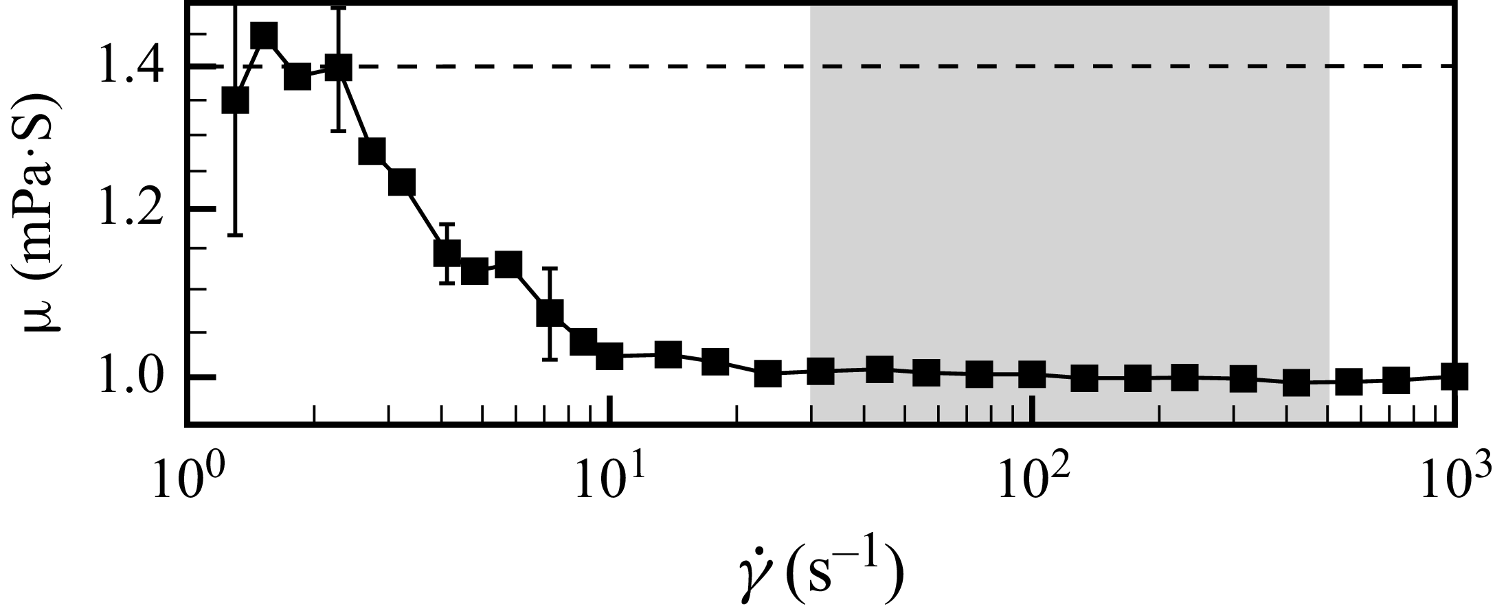
mm diameter). As an illustrative example, the mean dynamic viscosity for the
 $100$
ppm solution is plotted in figure 2. The shaded region indicates the range of wall shear rates encountered in the near-wall region across the various Reynolds numbers investigated in our experiments. Within this specific range, the viscosity remains nearly constant at
 $\mu \approx 1.00 \pm 0.04$
mPa s, exhibiting negligible shear-thinning. The density of the polymer solution was measured as
 $\rho = 0.9978 \pm 0.0005$
g cm−
 $^3$
using an Anton Paar densitometer (DMA35). Consequently, the kinematic viscosity of the
 $100$
ppm solution is determined to be
 $\nu \approx 1.00 \pm 0.04$
mm
 $^2$
s−1. This value is used to define the Reynolds number,
 $\textit{Re} = U_{\!B} D / \nu$
, following the standard protocols for dilute polymer solutions established in the literature (Metzner & Reed Reference Metzner and Reed1955; Draad, Kuiken & Nieuwstadt Reference Draad, Kuiken and Nieuwstadt1998; Ptasinski et al. Reference Ptasinski, Boersma, Nieuwstadt, Hulsen, van den Brule and Hunt2003; Samanta et al. Reference Samanta, Dubief, Holzner, Schäfer, Morozov, Wagner and Hof2013; Choueiri et al. Reference Choueiri, Lopez, Varshney, Sankar and Hof2021).
Dynamic viscosity of the polymer solution for the concentration of
 $100$
ppm against the shear rate
 $\dot {\gamma }$
. The grey area indicates the range of near-wall flow shear rates in this study.

As the shear rate
 $\dot {\gamma }$
decreases from approximately
 $10$
s
 $^{-1}$
, the dynamic viscosity
 ${\unicode{x03BC}}$
increases and reaches a well-defined plateau of approximately
 $1.4$
mPa s at
 $\dot {\gamma } \sim 1$
s
 $^{-1}$
. This constant value is identified as the zero-shear dynamic viscosity. The corresponding kinematic zero-shear viscosity is determined to be
 $\nu _0 \approx 1.4$
mm
 $^2$
s−1, which is further used to estimate the viscosity ratio
 $\beta = \nu _s / \nu _0$
. Here,
 $\nu _s$
represents the kinematic viscosity of the solvent and
 $\beta$
characterizes the relative contribution of the solvent to the total zero-shear viscosity of the polymer solution. The Weissenberg number,
 $Wi = \lambda U_{\!B} / D$
, quantifies the ratio of elastic to viscous forces and is widely adopted as a primary flow control parameter in numerical simulations of viscoelastic flows. For polymer solutions at concentrations
 $c = 100$
,
 $200$
,
 $300$
,
 $400$
and
 $500$
ppm, the shear relaxation time
 $\lambda$
was determined experimentally using the Anton Paar rheometer (MCR302), following the protocol outlined by Choueiri et al. (Reference Choueiri, Lopez, Varshney, Sankar and Hof2021). In brief, each sample was subjected to a steady shear rate of
 $\dot {\gamma } = 10$
s
 $^{-1}$
for
 $30$
s to establish a pre-stressed state, after which the rotation was abruptly halted and the time-dependent decay of the shear stress
 $\tau (t)$
was recorded. The relaxation time
 $\lambda$
was extracted by fitting the stress relaxation curve to the exponential model
 ${\tau (t)}/{\tau _0} = \exp \! (-{t}/{\lambda } )$
, where
 $\tau _0$
is the steady-state shear stress prior to cessation. The measured values are
 $\lambda \approx 9.8$
,
 $10.9$
,
 $12.5$
,
 $14.5$
and
 $16.9\,\mathrm{s}$
for
 $c = 100$
,
 $200$
,
 $300$
,
 $400$
and
 $500\,\mathrm{ppm}$
, respectively. For intermediate concentrations (
 $c = 25$
,
 $50$
,
 $75$
,
 $150$
,
 $250$
and
 $350$
ppm),
 $\lambda$
was estimated using the scaling model of Muthukumar (Reference Muthukumar1984). To assess solution stability and homogeneity, two additional batches of the master polymer solution were sampled after
 $5$
and
 $7$
days of rotational homogenisation. Identical rheological measurements were performed and the resulting dynamic viscosities showed no statistically significant deviation from the primary dataset. Furthermore, post-experiment samples, which were collected immediately after each flow trial, were re-measured for viscosity; no detectable change was observed compared with pre-trial measurements. These results confirm the chemical and rheological stability of the solutions over the experimental timeframe.
2.3. Friction factor measurements
Friction factors were measured for each experimental case. Two pressure taps (
 $1$
mm diameter) were drilled through the pipe wall perpendicular to the axis, separated by an axial distance of
 $L_{\Delta P} = 6D$
. These taps were connected to a differential pressure transducer (Validyne DP103, equipped with a
 $0$
–
 $22$
Pa range membrane) via short polyurethane tubes (inner diameter
 $2.5$
mm), as illustrated in the schematic in figure 1. Pressure drop data were temporally averaged to obtain the mean pressure drop
 $\Delta P$
for each Reynolds number. The Darcy friction factor
 $f$
was subsequently calculated using the Darcy–Weisbach equation
 $f = {2D \Delta P}/({L_{\Delta P} \rho U_{\!B}^2})$
, where
 $\rho$
is the fluid density. To provide a baseline, friction factors for Newtonian laminar and turbulent flows were also measured for reference. The friction factors are plotted in figure 3(a). In this figure, the MDR asymptote (
 $f = 2.36 \textit{Re}^{-0.58}$
, Virk et al. Reference Virk, Mickley and Smith1970) is denoted by a dotted line, the Blasius solution for Newtonian turbulence (
 $f = 0.316 \textit{Re}^{-0.25}$
) by a dash-dotted line and the Hagen-Poiseuille solution for laminar flow (
 $f = 64/\textit{Re}$
) by a long-dashed line. At
 $\textit{Re} \approx 11\,200$
, the friction factors for concentrations
 $c = 0$
–
 $350$
ppm (coloured squares) show a progressive decrease as
 $c$
increases, effectively reaching the MDR asymptote for
 $c \gtrsim 250$
ppm. For a fixed concentration of
 $c = 100$
ppm (solid black squares),
 $f$
decreases with increasing Reynolds number (
 $\textit{Re} \approx 5600$
–
 $28\,000$
) and approaches the MDR asymptote at
 $\textit{Re} \gtrsim 19\,000$
. To better quantify these results, the drag reduction percentage (
 $\textit{DR}\%$
) was calculated following Lopez et al. (Reference Lopez, Choueiri and Hof2019) as
 $\textit{DR} \%= ({f_{\!N} - f_{\!P}})/{f_{\!N}} \times 100\,\%$
, where
 $f_{\!N}$
and
 $f_{\!P}$
represent the friction factors for Newtonian and polymer-laden turbulence, respectively. The resulting
 $\textit{DR}\%$
is presented in figure 3(b), and its ratio to the theoretical maximum drag reduction,
 $\textit{DR}\% / \textit{MDR}\%$
, is shown in figure 3(c), where
 $\textit{MDR}\% = (f_{\!N} - f_{\!M}) / f_{\!N}$
and
 $f_{\!M}$
is the friction factor at the MDR asymptote.
(a) Friction factors
 $f$
as a function of Reynolds number
 $\textit{Re}$
. The coloured circles denote
 $f$
at
 $\textit{Re}=11\,200$
with polymer concentrations ranging from
 $0$
to
 $350$
ppm. The solid black squares and hollow black circles denote
 $f$
for
 $\textit{Re}$
ranging from
 $5600$
to
 $28\,000$
at
 $c=100$
ppm and
 $c=0$
ppm (Newtonian). (b) Corresponding drag reduction percent (
 $\textit{DR}\%$
). The dotted line denotes the MDR asymptote. (c) Ratio of
 $\textit{DR}\%$
to the MDR asymptote,
 $\textit{DR}\%/\textit{MDR}\%$
. The dashed lins denotes the unity, and the grey shaded line denotes the range
 $0.97\leqslant \textit{DR}\%/\textit{MDR}\%\leqslant 1.03$
, used as the criterion to identify whether the MDR asymptote has been reached. The three panels share the same legends.

To validate the pressure drop measurements, friction factors for
 $c = 0$
and
 $100$
ppm were additionally measured using a significantly larger tap separation of
 $64D$
. These measurements used the same differential pressure transducer (Validyne DP103) equipped with a higher-range diaphragm (
 $\#8$
–
 $14$
,
 $0$
–
 $220$
Pa). As illustrated in figure 3(a) by the magenta left-pointing triangles (Newtonian turbulence) and the cyan right-pointing triangles (polymer turbulence), the data obtained at the
 $64D$
spacing exhibit negligible deviations from the results recorded at the
 $6D$
separation. This agreement confirms the spatial development and consistency of the pressure gradient measurements.
3. Results
3.1. Fractal dimension of turbulent-kinetic-energy isosurfaces
The turbulent kinetic energy (TKE) is approximated using a two-dimensional surrogate, defined as
 $k \approx (u^{\prime 2} + v^{\prime 2})/2$
, where
 $u^{\prime } = u - \langle u \rangle$
and
 $v^{\prime } = v - \langle v \rangle$
represent the streamwise and wall-normal velocity fluctuations, respectively, with
 $\langle \boldsymbol{\cdot }\rangle$
denoting the ensemble spatial and temporal averages. To analyse the spatial distribution of the TKE, a specific threshold,
 $k^{\ast }$
, is applied to extract the corresponding isocontours in the two-dimensional measurement plane. Instantaneous snapshots of the TKE field are presented in figure 4(a) for the polymer pipe flow (
 $c = 100$
ppm,
 $\textit{Re} = 21\,000$
) and in figure 4(b) for the Newtonian pipe flow (
 $\textit{Re} = 20\,000$
). In the polymer pipe flow, the isocontour at
 $k^{\ast } = 0.0007$
bounds a large, contiguous domain, accompanied by scattered isolated pockets both inside and outside this primary region. Conversely, in the Newtonian pipe flow subjected to the same threshold, the energetic regions are highly fragmented, characterised by numerous small, disconnected domains. When the threshold is increased to
 $k^{\ast } = 0.0030$
, the isocontours for both cases isolate more coherent, contiguous core structures with a notable reduction in the number of surrounding fragmented pockets.
Contours of turbulent kinetic energy for (a) the polymer pipe flow at
 $\textit{Re}=21\,000$
and
 $c=100$
ppm and (b) the Newtonian turbulent pipe flow at
 $\textit{Re}=20\,000$
, where the red and blue solid lines denote the isolines of
 $k^{\ast }=0.0007$
and
 $k^{\ast }=0.0030$
, respectively.

(a) Averaged number of boxes
 $\langle N\rangle$
as a function of the box size
 $b$
for the Reynolds number
 $\textit{Re}=21\,000$
and the polymer concentration
 $c=100$
ppm at the threshold
 $k^{\ast }=0.0007$
. The inset shows
 $\langle N\rangle \boldsymbol{\cdot }(b/D)^{1.67}$
with a fitting curve (the solid line), where the dotted line marks a constant and the grey band illustrates the
 $3\,\%$
uncertainty of this constant. (b) Fractal dimension of polymer turbulence versus the threshold
 $k^*$
at
 $\textit{Re}=21\,000$
and
 $c=100$
ppm. The isolines of coarse-grained turbulent kinetic energy for (c) a small size of kernel
 $b_{\!f}$
and (d) a large one at the threshold
 $\tilde {k}^{\ast }=0.0007$
at
 $\textit{Re}=21\,000$
and
 $c=100$
ppm, using a box filter. (e) Corresponding length of the isolines
 $L_{\!f}$
versus the kernel size
 $b_{\!f}$
at
 $\tilde {k}^{\ast }=0.0007$
for the box and Gaussian filters.

The box-counting method is employed to determine the fractal dimension
 $D_F$
of the TKE isocontours, using a threshold of
 $k^* = 0.0007$
as a representative case. In this procedure, the
 $(x, y)$
measurement plane is partitioned into square boxes of side length
 $b$
, where
 $N(b)$
represents the number of boxes intersected by the TKE isocontours. As illustrated in figure 5, the ensemble-averaged number of boxes
 $\langle N \rangle$
follows a power-law scaling relationship,
 $\langle N \rangle \sim b^{-D_F}$
, as
 $b$
increases. To mitigate potential artefacts arising from discrete box-partitioning at larger scales (Feder Reference Feder2013; Wu et al. Reference Wu, Jin, Mi and Tang2020), only data points corresponding to
 $b = 2^n$
(where
 $n$
is an integer) are used for the fitting in the large-
 $b$
regime. Linear regression over the identified scaling range yields a fractal dimension of
 $D_F \approx 1.67$
for both the polymer and Newtonian pipe flows. To rigorously evaluate the scaling behaviour, the compensated number of boxes,
 $\langle N \rangle (b/D)^{1.67}$
, is plotted against the normalised scale
 $b/D$
, as shown in the inset of figure 5. As the scale
 $b$
increases, the compensated value asymptotically approaches a stable plateau. This plateau is represented by a dotted line, with a shaded grey band indicating a
 $\pm 3\,\%$
uncertainty interval. A second-order polynomial fit is conducted on the data points near the lower boundary of this grey band to identify the cross-over scale
 $b^*$
. In this representative case,
 $b^* \approx 0.055D$
, which significantly exceeds the aforementioned PIV noise-floor threshold (
 $\approx 0.01D$
). For scales larger than
 $b^*$
, the data remain consistently within the uncertainty band across a substantial range of
 $b$
. Furthermore, the
 $b^*$
values obtained through different uncertainty thresholds and fitting methodologies exhibit only negligible variations and do not affect the observed trends with respect to the flow control parameters (refer to the detailed discussion in § 4.1). This scale
 $b^*$
represents the characteristic cross-over length scale (e.g. Constantin et al. Reference Constantin, Procaccia and Sreenivasan1991; Grossmann & Lohse Reference Grossmann and Lohse1993; de Silva et al. Reference de Silva, Philip, Chauhan, Meneveau and Marusic2013), above which the TKE isocontours exhibit self-similarity, characterised by a nearly constant fractal dimension
 $D_F = 1.67 \pm 0.03$
. To assess the robustness of this result, the box-counting method was also applied to velocity fields obtained via the optical flow method. As illustrated in figure 15 of Appendix B, the data from the optical flow analysis nearly collapse onto the results from the PIV cross-correlation algorithm. This agreement indicates that the choice of vector extraction algorithm and the spatial resolution (vector spacing) have a negligible influence on the determined fractal dimensions. Further sensitivity analyses are provided in Appendix B. When a higher TKE threshold,
 $k^* = 0.002$
, is applied, a lower fractal dimension of
 $D_F \approx 1.56$
is observed. Systematic examination of various
 $k^*$
values reveals that
 $D_F$
remains approximately constant across a specific range of thresholds, as shown in figure 5(b). However, as
 $k^*$
increases beyond this range,
 $D_F$
exhibits a monotonic decay, demonstrating that the fractal dimension is ultimately dependent on the chosen threshold. This trend is consistent with previous findings regarding the fractal dimensions of passive scalar mixing in turbulent flows (e.g. Prasad & Sreenivasan Reference Prasad and Sreenivasan1990; Zhou & Xia Reference Zhou and Xia2010; Iyer et al. Reference Iyer, Schumacher, Sreenivasan and Yeung2020; Li, Xu & He Reference Li, Xu and He2025).
To ensure that the determined fractal dimension is independent of the extraction methodology, we employ the coarse-graining method (de Silva et al. Reference de Silva, Philip, Chauhan, Meneveau and Marusic2013). Following the analysis of the turbulent kinetic energy, the velocity fluctuation fields are filtered across various scales. A smoothing kernel with a characteristic length scale
 $b_{\!f}$
is used to filter the velocity fluctuations; for instance, the filtered horizontal velocity fluctuation is calculated as
 $\tilde {u^{\prime }}(x,y,t)=\iint u^{\prime }({x}-{x}^{\prime }, {y}-{y}^{\prime }, t) G_{b_{\!f}}({x}^{\prime },{y}^{\prime })\,\mathrm{d}{x}^{\prime }\,\mathrm{d}{y}^{\prime }$
, where
 $u^{\prime }$
is the instantaneous horizontal velocity fluctuation. Here,
 $G_{b_{\!f}}(x^{\prime },y^{\prime })$
denotes a two-dimensional (2-D) box filter defined such that
 $G_{b_{\!f}}(x^{\prime },y^{\prime })=1/b_{\!f}^2$
for
 $|x^{\prime }|, |y^{\prime }| \lt b_{\!f}/2$
, and
 $G_{b_{\!f}}=0$
otherwise. The filtered vertical velocity fluctuation
 $\tilde {v^{\prime }}({x},{y},t)$
is obtained in a similar manner and the resulting filtered turbulent kinetic energy is computed as
 $\tilde {k}=(1/2)(\tilde {u^{\prime }}^2+\tilde {v^{\prime }}^2)$
. It should be noted that the TKE fields derived directly from PIV are inherently filtered by the interrogation window size, reflecting the local averaging effects typical of PIV algorithms (Xu & Chen Reference Xu and Chen2013). Comparing figures 5(c) and 5(d), the isocontours clearly become smoother as
 $b_{\!f}$
increases, while their mean spatial positions remain largely unchanged. Following the approach of de Silva et al. (Reference de Silva, Philip, Chauhan, Meneveau and Marusic2013), we examine the total length of the isocontours,
 $L_{\!f}$
, as a function of the kernel size
 $b_{\!f}$
. Using a threshold of
 $\tilde {k}^{\ast }=0.0007$
,
 $L_{\!f}$
is determined by identifying connected regions and calculating their perimeters, followed by ensemble averaging over all snapshots. The observed scaling is approximately
 $-0.63\pm 0.05$
. At large
 $b_{\!f}$
, the data points deviate from this power-law behaviour. This deviation is attributed to flow anisotropy, which becomes significant at larger scales (de Silva et al. Reference de Silva, Philip, Chauhan, Meneveau and Marusic2013). Below this deviation threshold, large-scale self-similarity emerges (Mistry et al. Reference Mistry, Philip, Dawson and Marusic2016), suggesting that this scale serves as the upper bound for the self-similar regime. If the isocontours exhibit fractal behaviour, a scaling of
 $L_{\!f} \sim b_{\!f}^{1-D_L}$
is expected (de Silva et al. Reference de Silva, Philip, Chauhan, Meneveau and Marusic2013; Mistry et al. Reference Mistry, Philip, Dawson and Marusic2016), where
 $D_L$
represents the fractal dimension derived from the coarse-graining method. In our study, the scaling exponent
 $1-D_L \approx -0.63$
across various Reynolds numbers and thresholds yields
 $D_L \approx 1.63 \pm 0.05$
, which is in close agreement with the
 $D_F \approx 1.67$
obtained via the box-counting method. We further examined the application of a Gaussian kernel, which yielded a
 $D_L$
of approximately
 $1.63$
, consistent with the results from the box filter as shown in figure 5(e). The strong agreement between these two distinct methodologies indicates that the determined fractal dimension is independent of the computational method; further details are provided in § 4.1.
3.2. Effect of polymer concentration on the fractal dimension
In the previous section, we detailed the methodology for determining fractal dimensions using representative cases of both Newtonian and polymer turbulence. This section examines the influence of polymer concentration on the fractal dimension. To isolate the effects of viscoelasticity from inertial effects, the flow Reynolds number is held constant at
 $\textit{Re}=11\,200$
, while the polymer concentration is varied from
 $0$
ppm to
 $350$
ppm. Notably, as the polymer concentration increases, the degree of drag reduction rises towards the MDR asymptote, which is nearly reached at
 $c \approx 250$
ppm (see figures 3
b and 3
c). This systematic variation allows for a clear characterisation of how increasing viscoelasticity modulates the fractal scaling of the turbulence. A more comprehensive discussion of the correlation between the fractal dimension and drag reduction performance is provided in § 4. The specific flow parameters for all cases are summarised in table 1.
Flow parameters in this study:
 $\textit{Re}$
is the Reynolds number,
 $\beta$
is the ratio of the viscosity of the solvent to the zero-shear-rate viscosity of the polymer solution,
 $Wi$
is the Weissenberg number and
 $\eta$
is the Kolmogorov length scale. The estimation of
 $\beta$
and
 $Wi$
are provided to facilitate comparison among studies.

(a) Fractal dimension
 $D_F$
as a function of the polymer concentration
 $c$
at
 $\textit{Re}=11\,200$
. The horizontal dashed line indicates
 $D_F=1.67$
. The error bar denotes the uncertainty of the linear fitting log
 $(\langle N \rangle )$
with log(
 $b$
). The inset shows
 $D_F$
as a function of the threshold
 $k^*$
for three polymer concentrations. (b) The
 $b^{\ast }/D$
of the polymer pipe flows varies with
 $c$
. (c) Spatially averaged Kolmogorov length scale
 $\bar {\eta }$
of the polymer pipe flows, estimated using the PIV data with the local axisymmetry assumption. (d) Ratio
 $b^{\ast }/\bar {\eta }$
against
 $c$
. Here, the TKE threshold is
 $k^*=0.0007$
.

As demonstrated already, the fractal dimension exhibits a sensitive dependence on the TKE threshold. Consequently, it is challenging to isolate the influence of polymer concentration if both the threshold and the concentration are varied simultaneously. Accordingly, the TKE threshold is initially fixed at
 $k^* = 0.0007$
and the fractal dimension
 $D_F$
is calculated via the box-counting method for each concentration level. As shown in figure 6(a),
 $D_F$
decreases slightly as the concentration increases, gradually deviating from the theoretical value of
 $D_F \approx 1.67$
. Furthermore, for a given concentration (see the inset of figure 6
a),
 $D_F$
exhibits only a trivial or marginal sensitivity to the TKE threshold at low
 $k^*$
values; however, this dependence becomes more pronounced as
 $k^*$
increases, indicating that the fractal scaling is significantly affected by the threshold choice in high-energy regions of the flow.
The behaviour of the length scale
 $b^{\ast }$
is examined in figure 6(b). It demonstrates a gradual increase with rising polymer concentration up to
 $c \approx 250$
ppm, corresponding to the onset of the maximum drag reduction. Beyond this concentration,
 $b^{\ast }$
plateaus at
 $b^*/D \approx 0.09$
. As discussed in § 4.1, this trend is robust and remains insensitive to the choice of uncertainty thresholds and fitting methodologies employed to determine
 $b^*$
. Notably, Xi, Bodenschatz & Xu (Reference Xi, Bodenschatz and Xu2013) and Zhang et al. (Reference Zhang, Bodenschatz, Xu and Xi2021) investigated velocity structure functions in polymer-laden homogeneous isotropic turbulence generated within a von Kármán facility. They observed that the minimum length scale of the inertial range, analogous to our measured
 $b^*$
, also increases with polymer concentration. A key distinction in the present pipe flow study is the direct observation of drag reduction: once the concentration exceeds approximately
 $250$
ppm, the flow approaches the MDR asymptote, entering a saturated state where flow characteristics become largely independent of further increases in concentration. In the context of Newtonian turbulence, theories determining the fractal dimension mathematically bridge velocity structure functions with surface geometry, predicting
 $b^*$
to be approximately ten times the Kolmogorov length scale (Constantin et al. Reference Constantin, Procaccia and Sreenivasan1991; Grossmann & Lohse Reference Grossmann and Lohse1994). If this scaling holds for polymeric turbulence, an analogous intrinsic link between these two scales may exist. However, lacking theoretical extensions applicable to non-Newtonian frameworks, the exact nature of this connection remains unclear. Further theoretical development is required to rigorously define
 $b^*$
in viscoelastic flows, which falls beyond the scope of the present study.
As shown in figure 6(c), the spatially averaged Kolmogorov length scale,
 $\bar {\eta }$
, exhibits a trend similar to
 $b^*$
with respect to polymer concentration. The Kolmogorov scale is defined as
 $\eta = (\nu ^3/\epsilon )^{1/4}$
, where the TKE dissipation rate
 $\epsilon$
is estimated from two-dimensional PIV data based on the local axisymmetry assumption (Doron Reference Doron2001; Xu & Chen Reference Xu and Chen2013). Notably, estimations based on local isotropy were found to be consistent with those derived from the local axisymmetry assumption. The local values were then averaged over the measurement field-of-view to obtain
 $\bar {\eta }$
. The increase in the Kolmogorov scale reflects a decay in the dissipation rate, which occurs as a portion of the turbulent kinetic energy is transferred to and stored within the polymer molecules. This mechanism is consistent with the findings of Perlekar et al. (Reference Perlekar, Mitra and Pandit2006), Zhang & Xi (Reference Zhang and Xi2022) and Watanabe et al. (Reference Watanabe, Abreu, Nagata and da Silva2025), who observed that dissipation reduction intensifies with increasing concentration. Furthermore, the growth of
 $\bar {\eta }$
suggests the suppression of small-scale structures, the implications of which warrant further investigation from a fractality perspective. The variation of the ratio
 $b^{\ast }/\bar {\eta }$
is illustrated in figure 6(d). This ratio demonstrates a slight decrease as the concentration increases up to
 $250$
ppm, beyond which it remains approximately constant. A similar downward trend is evidenced by the ratio
 $l_L/\eta = (\lambda \nu /\eta ^2)^{3/2}$
, where
 $l_L = (\lambda ^3 \epsilon )^{1/2}$
is the Lumley length scale (Lumley Reference Lumley1969). The Lumley length represents the smallest length scale of the inertial range in viscoelastic flows (Vonlanthen & Monkewitz Reference Vonlanthen and Monkewitz2013), and its behavior suggests a relative shift in the scaling of small-scale structures as the polymer concentration approaches the MDR asymptote.
3.3. Effect of Reynolds number on the fractal dimension
This section investigates the effect of the Reynolds number on the fractal dimension. For this analysis, the polymer concentration is held constant at
 $c = 100$
ppm while the Reynolds number is systematically varied. As the Reynolds number increases, the drag reduction gradually approaches the MDR asymptote, which is nearly reached at
 $\textit{Re} \approx 19\,000$
. Unlike adjusting the polymer concentration, which modulates polymer elasticity without altering the bulk inertia, increasing the Reynolds number simultaneously amplifies both the inertial and elastic effects within the flow.
Following the previously established procedure, the fractal dimension
 $D_F$
is calculated for each Reynolds number at a fixed threshold of
 $k^*=0.0007$
, as presented in figure 7(a). The results indicate that, for the range of Reynolds numbers investigated here, the fractal dimension remains approximately constant (
 $D_F \approx 1.67$
) with only marginal fluctuations. This suggests that
 $D_F$
is effectively independent of
 $\textit{Re}$
across this regime. This analysis spans moderate Reynolds numbers, where drag reduction is partially realised, up to higher values (
 $\textit{Re} \gtrsim 19\,000$
) where the MDR asymptote is reached (see figure 3). In direct numerical simulations of polymeric channel flows, Dubief et al. (Reference Dubief, Terrapon and Soria2013) observed a
 $k^{-5/3}$
scaling within the inertial range of the velocity spectrum for elasto-inertial turbulence, matching the scaling found in Newtonian turbulent channel flows. If the theoretical link between the fractal dimension and the structure function, and consequently the power spectrum (Constantin et al. Reference Constantin, Procaccia and Sreenivasan1991; Grossmann & Lohse Reference Grossmann and Lohse1994), is assumed to hold for polymeric turbulence, the scaling reported by Dubief et al. (Reference Dubief, Terrapon and Soria2013) would imply a fractal dimension of approximately
 $1.67$
. A notable distinction, however, is that while spectral scaling is often poorly defined in turbulent flows with insufficient Reynolds numbers, the box-counting results exhibit a surprisingly robust and distinct scaling, even when a classical inertial range has not yet fully developed in the wavenumber domain. Admittedly, the precise connection between the fractal dimension and spectral scaling in polymeric turbulence remains somewhat ill-defined, given that a formal extension of fractal dimension theories to viscoelastic flows is currently unavailable.
(a) Fractal dimension
 $D_F$
of the polymer pipe flows versus the Reynolds number for Newtonian turbulence and polymer turbulence at
 $c=100$
ppm. The horizontal dotted line indicates
 $D_F=1.67$
. The error bar denotes the uncertainty of the linear fitting log
 $(\langle N \rangle )$
with log(
 $b$
). (b) The
 $b^{\ast }/D$
of the polymer pipe flows varies with
 $\textit{Re}$
, and the two dotted lines indicate the data trends
 $\textit{Re}^{-1/7}$
and
 $\textit{Re}^{-1/4}$
for eye guidance. (c) Spatially averaged Kolmogorov length scale
 $\bar {\eta }$
of the polymer pipe flows, obtained from the average of the Kolmogorov length scales estimated using the PIV data with the local axisymmetry assumptions. The two dotted lines indicate the power-law scaling trends of
 $\textit{Re}^{-3/5}$
and
 $\textit{Re}^{-1/4}$
for eye guidance. The inset shows the
 ${\eta _c}={\eta }(y/D=0)$
for the Newtonian pipe flows and the
 $\textit{Re}^{-3/4}$
scaling suggested by Cerbus et al. (Reference Cerbus, c. Liu, Gioia and Chakraborty2020) is shown as a dashed line. (d) Ratio
 $b^{\ast }/\bar {\eta }$
against
 $\textit{Re}$
, where the two dotted lines indicate the trends, respectively. Here the TKE threshold is
 $k^*=0.0007$
.

The variation of the length scale
 $b^{\ast }$
with the Reynolds number is presented in figure 7(b). As
 $\textit{Re}$
increases,
 $b^{\ast }$
decreases until
 $\textit{Re} \approx 19\,000$
. Beyond this point, the rate of decline slows, characterised by a transition bounded by the scaling relations
 $\textit{Re}^{-1/4}$
and
 $\textit{Re}^{-1/7}$
, as indicated by the two dotted lines in figure 7(b). For reference, Newtonian pipe flows exhibit a scaling of
 $b^* \sim \textit{Re}^{-1/5}$
. Similarly, the spatially averaged Kolmogorov length scale,
 $\bar {\eta }$
, is presented in figure 7(c). As shown in the inset, the estimated pipe-centre values for the Newtonian case, defined as
 $\eta _c = \eta (y/D=0)$
, closely agree with those reported by Cerbus et al. (Reference Cerbus, c. Liu, Gioia and Chakraborty2020). They recover an
 $\textit{Re}^{-3/4}$
scaling at the centreline, which is consistent with the classical dimensional relationship between viscous dissipation and large-scale turbulent motions (Taylor Reference Taylor1935). In the polymer pipe flows, the decay of
 $\bar {\eta }$
deviates from the Newtonian behaviour. For
 $\textit{Re} \lesssim 19\,000$
,
 $\bar {\eta }$
decreases more slowly than
 $\textit{Re}^{-3/4}$
and its decline becomes even more gradual for
 $\textit{Re} \gt 19\,000$
. This two-stage decay is approximately bounded by
 $\textit{Re}^{-3/5}$
and
 $\textit{Re}^{-1/4}$
, respectively, as indicated by the dotted lines in figure 7(c). It should be emphasised that these specific scaling exponents are not proposed as definitive universal laws; rather, they are presented simply to illustrate the distinct shift in the decay trend. Crucially, the continued variation of
 $b^*$
and
 $\bar {\eta }$
with increasing
 $\textit{Re}$
, even after the flow has reached the MDR state, contrasts sharply with the plateauing behaviour observed when increasing polymer concentration
 $c$
. This disparity provides strong evidence that increasing
 $\textit{Re}$
and increasing
 $c$
govern fundamentally different physical processes. Such a distinction likely stems from the growing dominance of bulk inertia, or from the complex, evolving interplay between inertial and elastic effects at high Reynolds numbers.
Lastly, the length scale ratio
 $b^*/\bar {\eta }$
is presented in figure 7(d). In the Newtonian case,
 $b^*/\bar {\eta }$
increases with
 $\textit{Re}$
, though the rate of growth gradually tapers off at higher Reynolds numbers. For the polymer-laden flows,
 $b^*/\bar {\eta }$
follows a power-law increase for
 $\textit{Re} \lt 19\,000$
, a trend consistent with the individual scaling behaviours of
 $b^*$
and
 $\bar {\eta }$
discussed previously. Within this relatively narrow range, the increase is approximately linear, as indicated by the dashed line in figure 7(d). For
 $\textit{Re} \gtrsim 19\,000$
, the ratio plateaus at an approximately constant value of
 $b^*/\bar {\eta } \approx 13$
, denoted by the horizontal dashed line. The saturation of
 $b^*/\bar {\eta }$
suggests that the turbulence within the pipe reaches a converged equilibrium state as it approaches the MDR asymptote. Using small-diameter pipes to achieve lower Reynolds numbers and presumably stronger viscoelastic effects, Choueiri et al. (Reference Choueiri, López and Hof2018) demonstrated that once the flow reaches the MDR asymptote, it is dominated by elasto-inertial turbulence. However, significant differences exist between the Reynolds number regimes and the corresponding magnitudes of the viscoelastic effects in the study by Choueiri et al. (Reference Choueiri, López and Hof2018) and the present work. Consequently, whether these two systems converge towards the same universal equilibrium state requires further empirical investigation. This could be addressed by conducting experiments in smaller diameter pipes or by employing alternative solvents (e.g. glycerine) to achieve comparable viscoelastic parameters. While the former remains technically challenging for high-resolution flow measurements due to spatial constraints, the latter is technically feasible, though it may substantially increase experimental costs for medium-scale facilities.
4. Discussions
4.1. Validation of configurations on extraction of fractal dimension
The fractal dimension determined by the box-counting method is further validated using the coarse-graining method. As shown in figure 8(a), the
 $L_{\!f}$
–
 $b_{\!f}$
curves for Reynolds numbers ranging from
 $11\,200$
to
 $21\,000$
(at
 $c = 100$
ppm) exhibit a robust collapse, characterised by a scaling exponent of approximately
 $L_{\!f} \sim b_{\!f}^{-0.63}$
. This indicates that the fractal dimension obtained via coarse-graining, denoted as
 $D_L$
, remains nearly invariant across the investigated Reynolds numbers, staying within the range
 $1.63 \pm 0.02$
. This result is highly consistent with the dimensions obtained from the box-counting analysis. Additionally, the
 $L_{\!f}$
–
 $b_{\!f}$
relationship was examined for different thresholds, specifically
 $\tilde {k}^{\ast } = 0.0005$
,
 $0.0007$
and
 $0.0009$
(at
 $c = 100$
ppm and
 $\textit{Re} = 21\,000$
), as presented in figure 8(b). The data again demonstrate a scaling close to
 $-0.63$
, corresponding to
 $D_L \approx 1.63$
, which confirms the robustness of the scaling regardless of the chosen threshold. To ensure the independence of the coarse-graining results from the specific filter type, the standard box filter was replaced with a Gaussian filter while maintaining all other parameters. Taking the velocity fluctuation
 $u^{\prime }$
as a representative variable, the Gaussian-filtered field
 $\tilde {u^{\prime }}(x,y,t)$
is defined as
 $\tilde {u^{\prime }}(x,y,t) = \iint u^{\prime }(x-x^{\prime }, y-y^{\prime }, t) K \exp [-({x^{\prime 2}+y^{\prime 2}})/({2\sigma ^2})] \,\mathrm{d}x^{\prime }\, \mathrm{d}y^{\prime }$
, where the filter kernel is localised within a square window of side length
 $b_{\!f}$
(i.e.
 $|x^{\prime }|, |y^{\prime }| \lt b_{\!f}/2$
) and is zero elsewhere. The standard deviation is set to
 $\sigma = b_{\!f}/6$
to ensure a cutoff radius of
 $3\sigma$
. The constant
 $K$
is a normalisation factor such that the integral of the kernel over the window equals unity. The resulting
 $L_{\!f}$
–
 $b_{\!f}$
curve in figure 8(c) closely follows the red dashed line representing the
 $-0.63$
scaling (
 $D_L \approx 1.63$
). This reinforcement highlights the methodological consistency between the coarse-graining and box-counting approaches.
The (a)
 $L_{\!f}/D$
as a function of
 $b_{\!f}/D$
at
 $\tilde {k}^{\ast }=0.0007$
at
 $c=100$
ppm. The black dashed line denotes a scaling of
 $-0.63\pm 0.02$
. The (b)
 $L_{\!f}/D$
as a function of
 $b_{\!f}/D$
at
 $\textit{Re}=21\,000$
for
 $\tilde {k}^{\ast }=0.0005$
,
 $0.0007$
and
 $0.0009$
. The red dashed line denotes a scaling of
 $-0.63\pm 0.05$
. (c) Comparison of the coarse-graining results using a box filter and a Gaussian filter, where the red dashed line denotes a
 $-0.63$
scaling.

The (a)
 $D_F$
and (b)
 $b^*$
as a function of polymer concentration for threshold
 $k^*=0.15\bar {k}$
. (c) Critical scale
 $b^*$
determined using polynomial fitting and uncertainty thresholds of
 $3\,\%$
(solid black diamonds),
 $4\,\%$
(solid blue downward triangles) and
 $5\,\%$
(solid red upward triangles) as a function of polymer concentration, where the lines are guides to the eye.

Given that the overall turbulent kinetic energy level varies with the flow control parameters, we evaluate an alternative criterion based on the spatially and temporally averaged TKE,
 $\bar {k}$
. This adaptive approach is demonstrated using the variable polymer concentration dataset, with the threshold set to
 $k^* = 0.15\bar {k}$
. As illustrated in figures 9(a) and 9(b), both
 $D_F$
and
 $b^*$
exhibit trends identical to those obtained using the fixed threshold
 $k^*=0.0007$
. This consistency indicates that our observations are robust and independent of the specific TKE thresholding criterion.
To further assess whether the value of
 $b^*$
is sensitive to the fitting configuration, we performed a sensitivity analysis on the plateau tolerance and the interpolation method applied to the
 $\langle N\rangle \boldsymbol{\cdot }(b/D)^{D_F}$
curves. We systematically varied the fitting method (comparing polynomial and spline fits) and the plateau tolerance threshold (
 $3\,\%$
,
 $4\,\%$
and
 $5\,\%$
) to verify the stability of the
 $b^*$
trend. As summarised in figure 9(c), the resulting trend of
 $b^*$
remains essentially invariant across different combinations of fitting methods and tolerance levels, thereby confirming the robustness of our characterisation of the length scale
 $b^*$
.
(a) Fractal dimension
 $D_F$
and
 $\overline {D'_F}$
as a function of the threshold
 $k^*$
for
 $c=100$
ppm and
 $\textit{Re}=11\,200$
. The grey area denotes the range of
 $1.67\pm 0.05$
. (b) Probability density function (p.d.f.) of the wall-normal positions of the isolines. (c) Profiles of
 $D_F^{\prime }(y)$
for four
 $k^*$
(sharing the same legend in panel b), where the grey area denotes the range of
 $1.67\pm 0.05$
.

4.2. Fractal dimension in space
The preceding analysis examines the fractal dimension of isolines extracted from 2-D velocity fields. The resulting 2-D fractal dimension,
 $D_F$
, provides a global characterisation of the flow structures, encompassing both spatial inhomogeneity and anisotropy. To further elucidate these effects, we examine the one-dimensional (1-D) fractal dimension,
 $D_F^{{\rm 1\text{-}D}}$
, calculated using the turbulent kinetic energy along the streamwise direction at discrete radial positions. Under the assumption of isotropy, the 2-D fractal dimension can be linked to the 1-D dimension through the additive law (Mandelbrot Reference Mandelbrot1983; Sreenivasan & Meneveau Reference Sreenivasan and Meneveau1986; Zhuang et al. Reference Zhuang, Tan, Huang, Liu and Zhang2018). Following the methodology of Sreenivasan & Meneveau (Reference Sreenivasan and Meneveau1986), we define an auxiliary dimension
 $D_F^{\prime } = D_F^{{\rm 1\text{-}D}} + 1$
. This shift maps the 1-D results onto a range comparable to the 2-D fractal dimension, facilitating a more direct comparison between the two. The variable
 $D_F^{\prime }$
is subsequently radially averaged to yield
 $\overline {D_F^{\prime }}$
. As an illustrative example, figure 10(a) demonstrates that for
 $(\textit{Re}, c) = (11\,200, 100\,\mathrm{ppm})$
, the dependence of
 $\overline {D_F^{\prime }}$
on the TKE threshold
 $k^*$
closely mirrors the trend of the 2-D fractal dimension
 $D_F$
. This resemblance motivates a closer examination of the preferential wall-normal locations of the
 $k^*$
isolines. Figure 10(b) shows that the probability density function (p.d.f.) profiles of these isolines shift significantly with
 $k^*$
. This confirms that isolines at different thresholds populate distinct radial regions of the pipe, implying that the 2-D fractal dimension
 $D_F$
primarily reflects the localised flow dynamics where these isolines are concentrated. To further support this, figure 10(c) illustrates the spatial variation of
 $D_F^{\prime }$
. Consistent with the p.d.f. profiles in figure 10(b), for
 $k^* \leqslant 0.0007$
, the local dimension
 $D_F^{\prime }$
attains its maximum at the pipe centreline and gradually decays radially outward. This spatial correlation between the local fractal dimension and isoline density substantiates the similarity between
 $\overline {D_F^{\prime }}$
and
 $D_F$
observed in figure 10(a). These lower fractal dimensions indicate that low-TKE isolines are relatively smoother near the wall and become increasingly ‘rougher’ towards the pipe centre (Frisch, Sulem & Nelkin Reference Frisch, Sulem and Nelkin1978). From a physical standpoint, this implies that for lower TKE levels, inter-scale energy transfer is less efficient near the wall but more effective at the pipe centreline. Conversely, for
 $k^* \geqslant 0.0020$
,
 $D_F^{\prime }$
reaches its minimum at the pipe centre and increases with the wall distance
 $y$
before exhibiting a slight decrease very close to the wall. This demonstrates that high-TKE isolines are relatively smoother in the core region and rougher near the wall, the opposite of the low-TKE behaviour. Analogously, the energy transfer for higher TKE levels appears to be more effective near the wall and less efficient at the pipe centre, contrasting sharply with the low-TKE dynamics.
(a) Contours of fractal dimension
 $D_F^{\prime }$
in the parameter space expanded by polymer concentration and radial position at
 $\textit{Re}=11\,200$
for
 $k^{\ast }=0.0007$
, and (b) corresponding profiles at
 $r/D=0$
(black circles),
 $0.20$
(blue diamonds) and
 $0.44$
(red circles). (e, f) Contours of fractal dimension
 $D_F^{\prime }$
and the corresponding profiles at
 $c=100$
ppm for
 $k^{\ast }=0.0007$
. Panels (c,d) and (g,h) are same as panels (a,b) and (e, f), respectively, for
 $k^{\ast }=0.0030$
.

While figure 10 provides spatial details of the fractal dimension, the influence of polymer concentration on its spatial variation warrants further investigation. We select two TKE thresholds,
 $k^*=0.0007$
and
 $0.003$
, as representative cases to map the auxiliary dimension
 $D'_F$
in the concentration–radial space, as shown in figure 11. These thresholds are chosen because they exhibit distinct characteristic profiles in figure 10(b). In figure 11(a), four iso-fractal-dimension lines (ranging from
 $D'_F = 1.52$
to
 $1.67$
) are presented. It can be observed that as the polymer concentration increases, the fractal dimension decreases gradually. Notably, this reduction reaches a state of saturation when the concentration exceeds approximately
 $250$
–
 $300$
ppm, the regime where the MDR asymptote is approached. Furthermore, as an example, the region defined by
 $D'_F \gt 1.67$
vanishes entirely as
 $D'_F$
saturates for
 $c \gt 200$
ppm. This suggests that upon reaching the MDR asymptote, the turbulence enters a distinct state where the fractal dimension differs fundamentally from that of Newtonian turbulence. To more clearly illustrate this trend, radial profiles at
 $r/D = 0$
,
 $0.2$
and
 $0.44$
are provided in figure 11(b). A similar saturation trend with increasing polymer concentration is observed for the higher threshold
 $k^*=0.003$
, as shown in figure 11(c,d). Specifically, the region characterised by large
 $D'_F$
is concentrated near the pipe wall at low concentrations; this region gradually shrinks and eventually disappears as concentration increases. For
 $c \gt 250$
ppm, corresponding to the MDR asymptote,
 $D'_F$
stabilises at approximately
 $1.5$
around
 $r/D = 0.4$
. Near the pipe centre,
 $D'_F$
remains below
 $1.4$
, indicating statistically smoother isolines in the core region.
Although only two TKE thresholds were presented as representative cases,
 $D'_F$
near the pipe wall consistently falls below
 $1.4$
across all thresholds. This indicates that as the flow approaches the MDR asymptote, near-wall turbulent structures become increasingly line-like in a 2-D cross-section. Physically, this implies the formation of extended, sheet-like structures within the streamwise–azimuthal plane, parallel to the wall. This structural interpretation, derived from the fractal dimension analysis, aligns well with observations from previous numerical simulations (Dubief et al. Reference Dubief, White, Shaqfeh and Terrapon2010, Reference Dubief, Terrapon and Soria2013). To better visualise these characteristics, the flow topologies rendered by the turbulent kinetic energy are presented in figure 12. These visualisations are constructed using Taylor’s hypothesis of frozen turbulence to facilitate a more comprehensive spatial representation along the pipe axis. The evolution of the TKE structures with increasing polymer concentration behaves qualitatively similarly to the trends reported in figures 2 and 4 of Choueiri et al. (Reference Choueiri, López and Hof2018). However, the structural modifications indicated by velocity fluctuations are relatively less pronounced in the present data. This discrepancy likely arises from the smaller pipe diameter used by Choueiri et al. (Reference Choueiri, López and Hof2018), where the correspondingly higher shear rates amplify the viscoelastic effects of the polymers. In contrast, the viscoelastic influence is inherently weaker in our larger-diameter facility. Although the higher Reynolds number in the present study promotes stronger polymer stretching, which partially compensates to achieve a comparable viscoelastic effect, the concomitantly enhanced inertial effects introduce unavoidable differences in the resulting flow structures.
Contours of TKE field obtained based on Taylor’s frozen hypothesis for (a)
 $c=0$
ppm, (b)
 $c=150$
ppm, (c)
 $c=250$
ppm and (d)
 $c=350$
ppm at
 $\textit{Re}=11\,200$
. The solid red and blue lines denote the isolines of
 $k^*=0.0007$
and
 $0.0030$
, respectively.

It is well established that the influence of polymers on turbulent shear flows results from a competition between viscoelastic effects and flow inertia (Xi Reference Xi2019). The viscoelastic effect, characterised by the polymer stress (Singh & Rosti Reference Singh and Rosti2025), is closely associated with the extent of polymer stretching – often evaluated via polymer conformation (e.g. Watanabe & Gotoh Reference Watanabe and Gotoh2013; Lopez et al. Reference Lopez, Choueiri and Hof2019; Steinberg Reference Steinberg2021) – and is therefore fundamentally linked to the local shear rate (Berti et al. Reference Berti, Bistagnino, Boffetta, Celani and Musacchio2006; White & Mungal Reference White and Mungal2008). Near the pipe centreline, the low shear rates resulting from both mean shear and velocity fluctuations lead to minimal polymer stretching. Consequently, inertial effects dominate the flow physics in this region. Conversely, near the pipe wall, the significant shear induces a dominant elastic effect, resulting in flow structures and energy spectra that differ markedly from those of Newtonian turbulence (Dubief et al. Reference Dubief, Terrapon and Soria2013; Thais, Mompean & Gatski Reference Thais, Mompean and Gatski2013; Shekar et al. Reference Shekar, McMullen, Wang, McKeon and Graham2019). Integrating these insights with the present fractal dimension observations, it can be concluded that a more pronounced viscoelastic effect leads to a reduction in both the local and radially averaged fractal dimensions. This reduction eventually saturates or reaches an equilibrium with other physical processes upon approaching the MDR asymptote. In contrast, stronger inertial effects produce more fragmented flow structures. This is supported by the observation that as the Reynolds number increases, the averaged fractal dimension remains nearly invariant. This plateau reflects a balanced competition between the enhanced viscoelastic effect (which tends to reduce the fractal dimension) and the increasing inertial effects (which tend to increase it). Based on this interpretation, a similar analysis of the 1-D fractal dimension was performed for varying Reynolds numbers. As shown in figure 11(e, f), at a TKE threshold of
 $k^*=0.0007$
, increasing the Reynolds number causes
 $D'_F$
at the pipe centre to rise gradually; simultaneously,
 $D'_F$
near the wall also increases and the region of low
 $D'_F$
diminishes. A similar trend is observed for the higher threshold
 $k^*=0.0030$
in figure 11(g,h): as the Reynolds number increases, a region of lower
 $D'_F$
emerges at the pipe centre, while a region of higher
 $D'_F$
develops near the wall. Although the MDR asymptote is nearly reached for
 $\textit{Re} \gt 19\,000$
, the spatial distribution of the fractal dimension remains distinctly different from the scenario where the MDR asymptote is achieved by increasing polymer concentration at a lower Reynolds number (
 $\textit{Re} \approx 11\,200$
), as documented in figure 11(a–d).
4.3. Fractal dimension and intermittency
The fractal dimension is fundamentally characterised by its capacity for ‘space-filling’ (Mandelbrot Reference Mandelbrot1975; Sreenivasan & Meneveau Reference Sreenivasan and Meneveau1986). Originally introduced to describe the multiscale nature of Newtonian turbulence, this concept is closely associated with small-scale intermittency (see Mandelbrot Reference Mandelbrot1975; Frisch et al. Reference Frisch, Sulem and Nelkin1978; Prasad & Sreenivasan Reference Prasad and Sreenivasan1990; Constantin et al. Reference Constantin, Procaccia and Sreenivasan1991; Iyer et al. Reference Iyer, Schumacher, Sreenivasan and Yeung2020). Intermittency is typically quantified by the departure of the scaling exponent
 $\xi$
from the classical
 $p/3$
prediction of Kolmogorov’s 1941 (K41) theory (Kolmogorov Reference Kolmogorov1991). Here,
 $\xi$
represents the scaling exponent of the
 $p$
th-order velocity structure function, defined as
 $\langle |\delta \boldsymbol{u}|^p \rangle \sim (\Delta x)^{\xi }$
, where
 $\delta \boldsymbol{u}$
is the velocity increment over a spatial separation
 $\Delta x$
. The magnitude of this deviation serves as a measure of the intermittency level; specifically, a smaller value of
 $\xi$
relative to the K41 prediction indicates more pronounced intermittency. For Newtonian homogeneous isotropic turbulence, the theoretical framework of Constantin et al. (Reference Constantin, Procaccia and Sreenivasan1991) relates the fractal dimension to the scaling exponent as
 $D_F = 2.5 + \xi (p=1)/2$
. This relationship demonstrates that, within the context of Newtonian turbulence, a lower fractal dimension
 $D_F$
implies stronger intermittency.
The degree of intermittency can also be quantified by the kurtosis
 $\mathcal{K}$
of the longitudinal velocity increment
 $\delta u^{\prime }$
(Pope Reference Pope2000; Singh & Rosti Reference Singh and Rosti2025), defined as
 \begin{equation} \mathcal{K}(\Delta x, y) = \frac {\langle (u^{\prime }(x+\Delta x, y) - u^{\prime }(x, y))^4 \rangle }{\langle (u^{\prime }(x+\Delta x, y) - u^{\prime }(x, y))^2 \rangle ^2} = \frac {\langle \delta u^{\prime 4} \rangle }{\langle \delta u^{\prime 2} \rangle ^2}. \end{equation}
For a Gaussian distribution of
 $\delta u^{\prime }$
, the kurtosis is
 $\mathcal{K} = 3$
(Pope Reference Pope2000). Deviations from this value, specifically
 $\mathcal{K} \gt 3$
, indicate that the p.d.f. of
 $\delta u^{\prime }$
possesses heavy tails, signifying the emergence of small-scale intermittency. In this study, the kurtosis is computed using the scale separation
 $\Delta x$
along the streamwise direction. To provide a clearer overview of the global trends, the kurtosis is radially averaged within the range
 $-0.4 \leqslant y/D \leqslant 0.4$
to obtain
 $\overline {\mathcal{K}}$
. At a constant Reynolds number of
 $\textit{Re} = 11\,200$
,
 $\overline {\mathcal{K}}$
for a given polymer concentration decreases monotonically as the scale separation
 $\Delta x$
increases, initially exhibiting a rapid decay followed by a more gradual decline at larger scales. As the polymer concentration
 $c$
is increased, the
 $\overline {\mathcal{K}}$
curves exhibit a distinct upward shift across all scales, indicating that the intensity of intermittency is enhanced by the presence of polymers. At a fixed concentration of
 $c = 100$
ppm, increasing the Reynolds number results in a marginal downward shift of the
 $\overline {\mathcal{K}}$
curve, suggesting a slight reduction in intermittency relative to the low-
 $\textit{Re}$
case. Similar trends regarding the sensitivity of kurtosis to polymer concentration and Reynolds number were recently reported for homogeneous isotropic polymeric turbulence by Singh & Rosti (Reference Singh and Rosti2025). Their findings further attribute this enhanced intermittency to the localised action of elastic stresses.
Kurtosis
 $\overline {\mathcal{K}}$
of the velocity fluctuation increment
 $\delta u^{\prime }$
along the streamwise direction: (a) three selected polymer concentrations at
 $\textit{Re}=11\,200$
; (b) three Reynolds numbers at
 $c=100$
ppm. The data points are skipped for clarity.

Synthesising our observations of the fractal dimension with the radially averaged kurtosis
 $\overline {\mathcal{K}}$
reveals that a reduction in
 $D_F$
correlates with an enhancement in the degree of intermittency. This inverse relationship is qualitatively consistent with the classical behaviour of Newtonian turbulence discussed earlier. In the framework of statistical turbulence, increased intermittency signifies a higher frequency of extreme or ‘rare’ events. We hypothesise that this enhanced intermittency in polymeric flows reflects more frequent transitions between distinct flow states. These transitions may manifest spatially, such as the switching between high-speed and low-speed streaks along the pipe axis as reported by Choueiri et al. (Reference Choueiri, López and Hof2018), or temporally such as the cycle between ‘hibernation’ and ‘active’ states described by Xi & Graham (Reference Xi and Graham2010) and Zhu & Xi (Reference Zhu and Xi2021). While these implications are compelling, rigorous verification remains necessary. Due to the limitations of the current measurement duration and the relatively moderate viscoelastic effects observed in this study, a definitive exploration of these state-switching dynamics is currently infeasible, and warrants future investigation with extended temporal datasets and higher polymer concentrations.
5. Concluding remarks
It is well established that the addition of polymer additives to turbulent pipe flows significantly reduces frictional drag. Concurrent with this drag reduction, the underlying turbulent structures undergo fundamental modifications induced by the presence of the polymers. Recent experimental and numerical investigations have highlighted the emergence of elasto-inertial turbulence and its critical relevance to the phenomenon of maximum drag reduction. This regime of turbulence is characterised by distinct flow structures that contrast sharply with those observed in Newtonian turbulence. In the present study, we adopt the framework of fractal geometry and fractal scaling to experimentally characterise turbulent polymer pipe flows. Our investigation explores two parameter spaces: varying the Reynolds number at a constant polymer concentration and adjusting the polymer concentration at a fixed Reynolds number. We find that the two-dimensional fractal dimension of the turbulent kinetic energy isosurfaces in Newtonian pipe flow is approximately
 $1.67 \pm 0.05$
. This value was determined using the box-counting method, and rigorously validated through coarse-graining techniques and alternative measurement configurations.
As the polymer concentration increases, the two-dimensional fractal dimension exhibits a marginal decrease; however, this trend is subtle and remains within the range of experimental uncertainty. We also examine the critical length scale, which defines the threshold beyond which the fractal dimension is extracted. Specifically, as the polymer concentration rises, the ratio of this critical length scale to the Kolmogorov scale decreases, eventually reaching an approximate plateau for concentrations exceeding
 $250$
ppm, a state corresponding to the MDR asymptote. As the Reynolds number increases, the 2-D fractal dimension remains nearly invariant. Concurrently, the ratio of the critical length scale to the Kolmogorov scale increases until it reaches a similar plateau for Reynolds numbers exceeding approximately
 $19\,000$
, where the MDR asymptote is again achieved. The emergence of this plateau in the scale ratio suggests that the turbulence has reached a state of statistical equilibrium, where inertial effects and viscoelastic forces are nearly balanced in their dynamical competition.
The spatial fractality of the turbulent structures is further analysed via the 1-D fractal dimension computed along the streamwise direction. As the polymer concentration increases, the distribution of this 1-D fractal dimension gradually evolves towards a saturation state upon reaching the MDR asymptote. This trend reinforces the conclusion that polymeric turbulence attains a state of asymptotic saturation within the MDR regime. We further examine the inter-relation between the fractal dimension and intermittency, observing that a reduction in the fractal dimension correlates with enhanced intermittency. While the intermittency remains nearly invariant and changes only marginally with increasing Reynolds number, it exhibits a pronounced increase as the polymer concentration rises. This clear enhancement in intermittency suggests a higher frequency of transitions between disparate turbulence states, occurring either spatially or temporally. Such transitions, which manifest as rare events under low-concentration conditions, become significantly more prevalent as the viscoelastic effects intensify.
In this study, we characterise classical polymeric turbulent pipe flows through the lens of fractal dimensions, a perspective that, while widely established in other areas of turbulence research, provides a novel framework for this specific problem. By varying the polymer concentration at a fixed bulk Reynolds number, we effectively isolate the viscoelastic effects. Our results demonstrate that the fractal dimension exhibits evidence of convergence within the maximum drag reduction regime at the selected Reynolds number. In contrast, recent numerical simulations by Zhu & Xi (Reference Zhu and Xi2021) at lower Reynolds numbers suggest that the flow state remains unconverged within an EIT-dominated MDR. This discrepancy underscores the inherent dynamical complexity of the MDR, which is increasingly understood to encompass multiple competing flow states (e.g. Zhu & Xi Reference Zhu and Xi2021; Wang et al. Reference Wang, Zhang, Wang, Li, Zhang and Li2023). Given the experimental challenges in directly measuring polymer stress fields, we cannot conclusively determine whether the MDR observed in our experiments is driven primarily by EIT or non-EIT dynamics. Future investigations into the fractal dimensions of flows where the dominant MDR dynamics are previously identified would help establish whether fractal scaling can serve as a robust indicator to distinguish between EIT and non-EIT regimes. While such a characterisation may be readily achievable in numerical simulations, experimental progress remains predicated upon the development of advanced measurement techniques capable of directly capturing three-dimensional vortical structures or localised polymer stresses.
Acknowledgements
D. Xu would like to thank Professor H. Xu (Tsinghua University), Professor J. Xie (Peking University) and Dr H. Li (Institute of Mechanics, Chinese Academy of Sciences) for the valuable discussions. The authors extend their thanks to Zongming Xie for his contribution to the initial set-up.
Funding
This work was supported by the National Natural Science Foundation of China (Grant Nos. 92152106, 12372224, 12588201 and 11988102) and the Chinese Academy of Sciences (Project for Young Scientists in Basic Research, Grant No. YSBR-087 and Strategic Priority Research Program, Grant No. XDB0620102).
Declaration of interests
The authors report no conflict of interest.
Author contributions
H.L. conducted the experiments, took the data analysis and prepared the figures, as well as wrote and reviewed the manuscript. D.X. conceptualised the study, analysed the data, and wrote and reviewed the manuscript.
Data availability statement
The data that support the findings of this study are available from the corresponding authors upon reasonable request.
Appendix A. Validation of statistical stationarity
The statistical convergence of the velocity fields has been rigorously verified. Taking the case of
 $c=0$
ppm at
 $\textit{Re} \approx 11\,200$
as a representative example, approximately
 $10\,000$
velocity fields were divided into three temporal subsets. The mean streamwise velocity profiles,
 $\langle U \rangle$
, were calculated for each individual subset and compared against the global average derived from the full dataset. As illustrated in figure 14(a), these profiles exhibit excellent collapse onto the
 $\langle U \rangle$
profile averaged over all snapshots, and both the upper and lower halves of the pipe (indicated by the solid black line). A similar validation was performed for the root-mean-square (r.m.s.) streamwise velocity fluctuations,
 $u^{\prime }_{\textit{rms}}$
. As shown in figure 14(c), the profiles from the subsets collapse onto the result obtained from the complete ensemble averaged over both pipe halves. The consistency observed in both
 $\langle U \rangle$
and
 $u^{\prime }_{\textit{rms}}$
confirms the statistical stationarity and axisymmetry of the streamwise velocity. Corresponding profiles for the
 $c=350$
ppm case at
 $\textit{Re} \approx 11\,200$
are presented in figures 14(b) and 14(d), respectively. These results likewise demonstrate statistical stationarity and axisymmetry. The fractal dimension
 $D_F$
and the critical length scale
 $b^*$
were calculated for each temporal subset; the values are remarkably consistent across subsets, as documented in table 2.
The
 $D_F$
and
 $b^*$
calculated for each
 $1/3$
partition of time series, for the cases of the minimum concentration
 $c=0$
ppm and the maximum concentration
 $c=350$
ppm at
 $\textit{Re}\approx 11\,200$
.

Profiles of (a,b)
 $\langle U \rangle$
and (c,d)
 $u^{\prime }_{\textit{rms}}$
for (a,c)
 $(\textit{Re},c)=(11\,200,0\,\mathrm{ppm})$
and (b,d)
 $(\textit{Re},c)=(11\,200,350\,\mathrm{ppm})$
. Grey-filled circles, cyan-filled diamonds and orange-filled squares denote the results over the first
 $1/3$
, the second
 $1/3$
and the last
 $1/3$
partition of the time series, respectively. Blue right and green left triangles denote the results of all snapshots at
 $x/D=0$
and
 $x/D=1$
, respectively. The solid black line denotes the result from all snapshots and averaged over both the upper and bottom halves of the pipe. Symbols are omitted for clarity.

The measurement field-of-view is positioned approximately
 $210D$
from the pipe entrance, a distance at which the turbulence is expected to be fully developed. The velocity statistics are independent of the streamwise location, as demonstrated hereafter. For each experimental case, the primary velocity statistics, namely the mean streamwise velocity
 $\langle U \rangle$
and the root-mean-square fluctuations
 $u^{\prime }_{\textit{rms}}$
, remain invariant with respect to the streamwise position. Representative profiles of
 $\langle U \rangle$
and
 $u^{\prime }_{\textit{rms}}$
for the cases of
 $c=0$
ppm and
 $c=350$
ppm are presented in figure 14. The profiles at the upstream boundary (
 $x/D=0$
) and the downstream boundary (
 $x/D=1$
) of the FOV virtually coincide, confirming that the turbulence is fully developed within our measurement region and that the statistics are streamwise-invariant.
Appendix B. Validation of velocity measurement configurations on fractal dimension extraction
Two validation trials were conducted to evaluate the influence of the extraction methodology and experimental configuration on the resulting fractal dimension. The first trial involved performing the experiments with a high-resolution camera (full sensor resolution of
 $9344 \times 7000$
pixels at a sampling rate of
 $71$
frames per second) equipped with a
 $100$
mm lens. To enhance spatial resolution, the field-of-view (FOV) was restricted to approximately
 $1D \times 1D$
at a resolution of
 $4096 \times 4096$
pixels, which allowed for a higher effective sampling rate. The camera was operated in double-frame, double-exposure mode, with external triggers used to acquire image pairs at a frequency of
 $25$
Hz. For the validation case at
 $c=100$
ppm and
 $\textit{Re}=28\,000$
, the time interval (pulse separation) within each image pair was set to
 $0.8$
ms. This specific Reynolds number, the maximum considered in this study, was selected for validation as it represents the most significant challenge to the measurement configuration. The velocity fields were processed using a multi-step cross-correlation algorithm, using a final interrogation window of
 $32 \times 32\,\mathrm{pixels}^2$
with a
 $50\,\%$
overlap.
The box-counting results
 $\langle N\rangle$
and compensated
 $\langle N\rangle$
(i.e.
 $\langle N\rangle (b/D)^{1.67}$
) are plotted in figures 15(a) and 15(b), respectively. Limited by the discretisation in the box-counting method, only the
 $2^n$
th points are presented for large
 $b/D$
(Feder Reference Feder2013; Wu et al. Reference Wu, Jin, Mi and Tang2020), where
 $n$
is an integer. The compensated
 $\langle N\rangle$
reaches a plateau at large
 $b/D$
, denoted by the blue dotted line, showing that the high-resolution PIV results give a fractal dimension of approximately
 $1.67$
, close to the result from the high-speed camera measurements (see the black dots, the results presented in the main text).
The (a)
 $\langle N\rangle$
as a function of
 $b/D$
for
 $c=100$
ppm and
 $\textit{Re}=28\,000$
. The blue down-triangles, black circles and red up-triangles correspond to the results from the PIV algorithm with image resolution of
 $4096\times 4096$
pixels
 $^2$
(
 $1D\times 1D$
,
 $32 \times 32\,\mathrm{pixels}^2$
with
 $50\,\%$
overlap, taken by the high-resolution camera), the PIV algorithm with image resolution of
 $2016\times 2016\,\mathrm{pixels}^2$
(
 $1.48D\times 1.48D$
,
 $32 \times 32\,\mathrm{pixels}^2$
with
 $75\,\%$
overlap, taken by the high-speed camera) and optical flow method which is based on PIV data from the high-speed camera configuration. (b) The
 $\langle N\rangle$
compensated by
 $(b/D)^{1.67}$
. The dotted lines are plotted in blue, black and red to denote the respective plateaus. The legends are the same as panel (a).

The optical flow method was also employed to estimate the velocity fields as a secondary validation of the cross-correlation-based PIV results. Optical flow represents the apparent motion of brightness patterns between consecutive image frames. A rigorous quantitative relationship between optical flow and fluid motion was established by Liu & Shen (Reference Liu and Shen2008) based on the intensity transport equation,
 ${\partial g}/{\partial t} + \boldsymbol{\nabla }\boldsymbol{\cdot }(g \boldsymbol{u}) = f(x,y,g)$
, where
 $g$
denotes the image intensity,
 $\boldsymbol{u}$
is the optical flow velocity vector field,
 $\boldsymbol{\nabla}$
represents the spatial gradient, and
 $f(x,y,g)$
accounts for boundary and diffusion effects (a detailed physical interpretation is provided in their original work). For this analysis, we used the open-source software OpenOpticalFlow (Liu Reference Liu2017). Because the optical flow method is most accurate for sub-pixel and small displacements (typically
 ${\lt}\ 5$
pixels), a predictor-corrector approach was implemented. The initial image was warped using the coarse velocity field obtained from the PIV analysis (
 $2016\times 2016\,\mathrm{pixels}^2$
FOV,
 $1.48D\times 1.48D$
, with
 $32 \times 32\,\mathrm{pixels}^2$
windows and
 $50\,\%$
overlap). This warping procedure ensured that the residual particle displacement was within the optimal
 $5$
-pixel range. The final velocity field was then calculated as the sum of the coarse PIV displacement and the fine-scale optical flow correction, with the PIV velocity assumed constant within each
 $8 \times 8\,\mathrm{pixels}^2$
sub-window. The resulting box-counting counts
 $\langle N\rangle$
and the compensated values
 $\langle N\rangle (b/D)^{1.68}$
, derived from the TKE fields calculated via optical flow, are plotted in figures 15(a) and 15(b), respectively. Consistent with the previous methodology, only points corresponding to
 $b/D = 2^n$
are shown for large box sizes. The
 $\langle N\rangle$
and compensated profiles obtained from the optical flow method exhibit an excellent collapse onto the corresponding PIV results. Furthermore, the compensated data converge to a clear plateau at large
 $b/D$
, confirming the high reliability of the PIV-derived velocity fields used throughout the main text.
This validation demonstrates that the PIV algorithm and vector-spacing used here do not affect the results.