

1 Introduction
Vortex reconnection is a fundamental topology-transforming dynamical event, playing a significant role in turbulence phenomena, such as energy cascade, fine-scale mixing (Hussain Reference Hussain1986) and noise generation (Zaman & Hussain Reference Zaman and Hussain1980). Vortex reconnection has also been implicated in flow transition and skin-friction jump in wall-bounded flows (Bake, Meyer & Rist Reference Bake, Meyer and Rist2002; Zhao, Yang & Chen Reference Zhao, Yang and Chen2016). In addition to its physical relevance, reconnection also represents a stand-alone mathematical problem related to the presence of finite-time singularity (FTS) of Euler or Navier–Stokes equations (Kerr Reference Kerr1993; Constantin, Fefferman & Majda Reference Constantin, Fefferman and Majda1996; Moffatt Reference Moffatt2000; Kerr Reference Kerr2018). Hence, vortex reconnection has been extensively studied over recent decades, both in classical (Ashurst & Meiron Reference Ashurst and Meiron1987; Melander & Hussain Reference Melander and Hussain1988; Kida, Takaoka & Hussain Reference Kida, Takaoka and Hussain1991; Kida & Takaoka Reference Kida and Takaoka1994; Hussain & Duraisamy Reference Hussain and Duraisamy2011) and in quantum (Koplik & Levine Reference Koplik and Levine1993; Bewley et al. Reference Bewley, Paoletti, Sreenivasan and Lathrop2008; Zuccher et al. Reference Zuccher, Caliari, Baggaley and Barenghi2012; Fonda, Sreenivasan & Lathrop Reference Fonda, Sreenivasan and Lathrop2019) turbulence.
As for viscous vortex reconnection, prior studies have mainly focused on relatively simple configurations: vortex rings (Kida et al. Reference Kida, Takaoka and Hussain1991), orthogonal vortices and colliding dipoles (Melander & Zabusky Reference Melander and Zabusky1988; Boratav, Pelz & Zabusky Reference Boratav, Pelz and Zabusky1992; Orlandi, Pirozzoli & Carnevale Reference Orlandi, Pirozzoli and Carnevale2012; Jaque & Fuentes Reference Jaque and Fuentes2017) and anti-parallel vortices with a sinusoidal perturbation of the axis introduced to force them to collide via self-induction. Reconnection physics of two vortices should be independent of the initial spatial configuration, as two vortex filaments with arbitrary orientations tend to become anti-parallel by mutual induction as they approach each other (Siggia Reference Siggia1985). Hence, we mainly focus on the reconnection of two anti-parallel vortex tubes subject to a sinusoidal displacement. Pumir & Kerr (Reference Pumir and Kerr1987) performed the first direct numerical simulation (DNS) study of such a configuration using the pseudospectral method, which mainly addressed the approach phase before reconnection. Soon after, Melander & Hussain (Reference Melander and Hussain1988) (hereinafter cited as MH) considered a more carefully designed initial vortex geometry to enable clearer insights into the mechanism details (this geometry has been extensively adopted by many other researchers). They, for the first time, highlighted three significant stages of reconnection: inviscid advection, bridging and threading (note that, until their study, reconnection was universally assumed to be complete in one stage leaving no remnant thread). Kerr & Hussain (Reference Kerr and Hussain1989) conducted a DNS study up to  $Re$
 $(\equiv \unicode[STIX]{x1D6E4}/\unicode[STIX]{x1D708},\text{circulation}/\text{viscosity})=3200$ by employing symmetry to reduce the computational requirement. They found a significant increase, as
 $Re$ increases, in the peak vorticity, suggesting a possible FTS of the Euler equations. Saffman (Reference Saffman1990) proposed a phenomenological model of reconnection employing an axial pressure gradient perspective to drive reconnection. Moreover, the model assumes that the strain rate is constant in the interaction region. However, this assumption is contrary to the numerical results, where the strain rate in the interaction region varies strongly in both space and time. Shelley, Meiron & Orszag (Reference Shelley, Meiron and Orszag1993) performed simulations with an adaptive spectral method on a stretched grid for
 $Re$ ranging from
 $500$ to
 $3500$ and compared their results with the Saffman model. They found that the reconnection time (
 $T_{R}$), defined as the time to halve the circulation on the symmetric plane, varies with
 $Re$ slower than the logarithmic variation suggested by the Saffman model. Note that they considered reconnection of two anti-parallel vortices, each consisting of a core of one vorticity surrounded by a sheath of opposite-signed vorticity; the inherent internal cancellation of vorticity at the interface renders such configuration highly pathological.
Kerr (Reference Kerr1993) performed the Euler simulation of a similar configuration with a particular interest in providing evidence of the FTS. However, it was shown by Hou & Li (Reference Hou and Li2006), later confirmed by Kerr (Reference Kerr2013a), that the maximum vorticity does not grow faster than double exponential in time; this precludes the possibility for FTS with this configuration. Hussain & Duraisamy (Reference Hussain and Duraisamy2011) (hereinafter cited as HD) systematically studied the mechanism of anti-parallel vortex reconnection up to  $Re=9000$. They found that the reconnection time scales as
 $Re^{-3/4}$, and the separation distance scales as
 $(t_{0}-t)^{3/4}$ and
 $(t-t_{0})^{2}$ before and after reconnection, respectively, where
 $t_{0}$ is the time when the centres are the closest. Van Rees, Hussain & Koumoutsakos (Reference van Rees, Hussain and Koumoutsakos2012) performed the simulation of the same configuration at
 $Re=10\,000$ with and without axial flow using the vortex method. They found that the energy spectrum during reconnection has a slope of
 $-5/3$ for the case without initial axial flow. In addition, the presence of axial flow was also found to affect the reconnection process, where the energy spectrum exhibits a
 $-7/3$ slope. Ni et al. (Reference Ni, Hussain, Wang and Chen2012) theoretically analysed the reconnection process for the anti-parallel configuration and predicted that the reconnection time varies continuously with
 $Re$ from
 $T_{R}\sim Re^{-1}$ at low
 $Re$ to
 $T_{R}\sim Re^{-1/2}$ at high
 $Re$. Beardsell, Dufresne & Dumas (Reference Beardsell, Dufresne and Dumas2016) visualized the simulation up to
 $Re=9000$ and observed the formation of ring-like structures based on vortex lines. They also found that the reconnection time agrees well with the scaling proposed by Ni et al. (Reference Ni, Hussain, Wang and Chen2012). Recently, McGavin & Pontin (Reference McGavin and Pontin2018) addressed the topological aspect of vortex reconnection, revealing some interesting features of the reconnection process, including the generation of many small vortex rings. For all these recent moderate-
 $Re$ (i.e.
 ${\leqslant}10\,000$) studies, the onset of symmetry breaking due to the Kelvin–Helmholtz (planar jet) instability is observed in the late stage of the reconnection, obscuring the essential mechanism of reconnection.
It is well accepted that energy is continuously transferred from energy-containing large scales to energy-dissipative smaller scales, which are statistically independent of the large-scale structures at high Reynolds numbers. Kolmogorov (Reference Kolmogorov1941) derived that the slope of the energy spectrum in the inertial range follows  $-5/3$, which has also been supported by many experimental and numerical studies. However, the physical mechanism of the energy cascade is hardly understood. Lundgren (Reference Lundgren1982) theoretically derived a structural model in the form of a spiraling vortex sheet for high-
 $Re$ turbulence. Although spiral vortex sheets can occur at places in the turbulent flows (Horiuti & Fujisawa Reference Horiuti and Fujisawa2008), their preponderance has never been found. Inspired by the previous work of Melander & Hussain (Reference Melander and Hussain1993) for vortex–turbulence interaction, Goto, Saito & Kawahara (Reference Goto, Saito and Kawahara2017) proposed a physical-space energy cascade mechanism for homogeneous isotropic turbulence: the energy cascade is caused by the successive creation of smaller-scale anti-parallel vortex tubes in the strain field induced by larger-scale vortex pairs. However, due to the complexity of the flow, the direct connection between the physical mechanism of the energy cascade and the statistics is not at all clear. For a better understanding of the energy cascade, one must examine well-defined simple vortical flows (Orlandi et al. Reference Orlandi, Pirozzoli and Carnevale2012). Based on low-
 $Re$ DNS and the knowledge of vortex dynamics, MH proposed a physical mechanism of energy cascade based on successive vortex reconnections. They found that, in contrast to the quantum reconnection, vortex reconnection in classical fluids is not complete – parts of the initial vortical tubes are left behind as vortex threads. At high
 $Re$, after the bridges have moved sufficiently apart, the mutual induction between the two adjacent threads would overcome the thrust of the weakened jet between the bridges causing the two threads to approach and collide again, starting the next round of reconnection. This process can repeat successively for sufficiently high
 $Re$. Recently, Brenner, Hormoz & Pumir (Reference Brenner, Hormoz and Pumir2016) also proposed an energy cascade mechanism based on the interaction of two anti-parallel vortex filaments: the vortex filaments flatten into extremely thin vortex sheets, which can break up into smaller vortex filaments due to instability; these filaments then collide, flattening and breaking up into even thinner filaments. The mechanism was demonstrated experimentally by McKeown et al. (Reference McKeown, Ostilla-Mónico, Pumir, Brenner and Rubinstein2018) through the head-on collision of two laminar vortex rings.
It is particularly noteworthy that despite interest in reconnection at high  $Re$, most studies so far have been limited to
 $Re\leqslant 10\,000$. The objective of the present study is not just to extend the
 $Re$ range to higher values, even moderately, but also to further shed light on the reconnection cascade scenario proposed by MH. In the next section, we discuss the details of the initial configuration and numerical set-up. The reconnection results, including flow visualization, separation distance and energy spectrum, at
 $Re=9000$ and higher
 $Re$ (i.e. 20 000 and 40 000) are discussed in §§ 3 and 4, respectively. Conclusions are drawn in § 5.
2 Initial configuration and numerical set-up
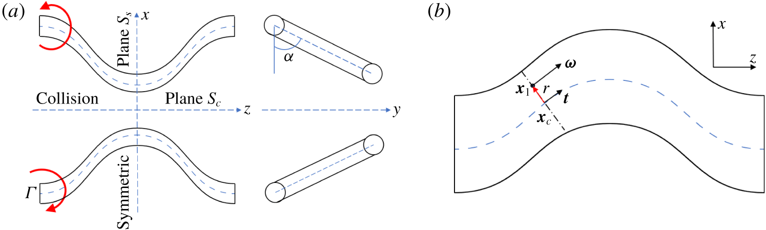
(a) Schematic of the initial configuration for anti-parallel vortex tubes, also showing the symmetry  $S_{s}$ and collision
 $S_{c}$ planes. (b) Illustration of circulation calculation in the plane perpendicular to the vortex axis.

We study the interaction of two sinusoidally displaced anti-parallel vortex tubes using the initial condition similar to that of MH (figure 1a). Note that the original initial configuration employed by MH does not strictly satisfy the Helmholtz theorem (the circulation is not conserved along the vortex tube axis; see appendix A for details). To ensure circulation conservation, minor modifications, similar to those of Kerr (Reference Kerr2013b), have been made here for the initial condition. For the perturbed vortex tube, the position of the initial vortex core is characterized by
 $$\begin{eqnarray}\displaystyle \boldsymbol{x}_{c}(s)=(x_{c}(s),y_{c}(s),s) & & \displaystyle\end{eqnarray}$$
with
 $$\begin{eqnarray}\displaystyle & \displaystyle x_{c}(s)=x_{0}+pf(s)\cos \unicode[STIX]{x1D6FC}, & \displaystyle\end{eqnarray}$$
 $$\begin{eqnarray}\displaystyle & \displaystyle y_{c}(s)=y_{0}+pf(s)\sin \unicode[STIX]{x1D6FC}, & \displaystyle\end{eqnarray}$$
where  $(x_{0},y_{0})$ denotes the initial position of the unperturbed vortex centroid,
 $p$ the amplitude of axis displacement and
 $\unicode[STIX]{x1D6FC}$ the inclination angle. To be consistent with the previous studies of MH and HD, we use
 $(x_{0},y_{0})=(\pm 0.81,0),\unicode[STIX]{x1D6FC}=60^{\circ },p=0.2$ and
 $f(s)=\cos (s)$.
Each vortex has a circular cross-section with
 $$\begin{eqnarray}\displaystyle \unicode[STIX]{x1D714}(r)=\left\{\begin{array}{@{}ll@{}}20[1-g(r/r_{c})],\quad & \text{if }r\leqslant r_{c}\\ 0,\quad & \text{otherwise},\end{array}\right. & & \displaystyle\end{eqnarray}$$
where  $g(r)=\exp [-Kr^{-1}\exp (1/(r-1))]$,
 $r_{c}=2/3$ and
 $K=1/2\exp (2)\log (2)$. Note that we use a compact support vorticity profile as the initial condition in order to prevent the peripheral region of the vortex from reconnecting so that the reconnection is more focused. The overall dynamics hereinafter is not restricted to this particular initial condition; we demonstrate this assertion by using a different initial condition: the Gaussian profile (see appendix B for details).
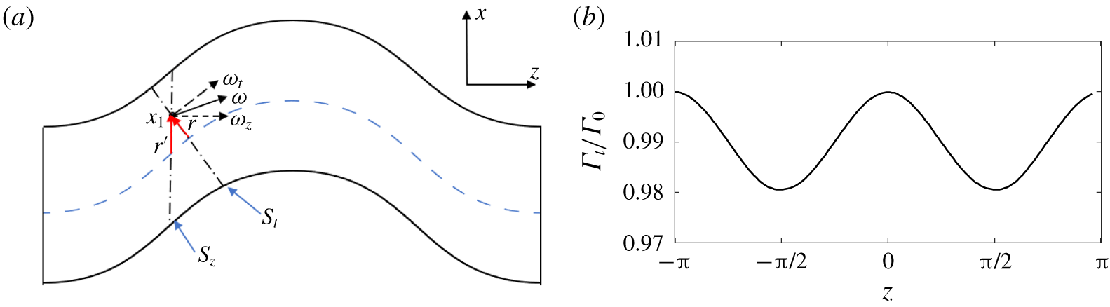
For a given point  $\boldsymbol{x}_{\mathbf{1}}=(x_{1},y_{1},z_{1})$, the radius
 $r$ is defined as the shortest distance between this point and the vortex core (figure 1b):
 $$\begin{eqnarray}\displaystyle r=\sqrt{(x_{1}-x_{c}(s_{1}))^{2}+(y_{1}-y_{c}(s_{1}))^{2}+(z_{1}-s_{1})^{2}}, & & \displaystyle\end{eqnarray}$$
where  $s_{1}$ is determined through
 $$\begin{eqnarray}\displaystyle \boldsymbol{t}\cdot [x_{1}-x_{c},y_{1}-y_{c},z_{1}-s_{1}]=0, & & \displaystyle\end{eqnarray}$$
with  $\boldsymbol{t}$ the tangent vector for the closest point
 $\boldsymbol{x}_{c}(s_{1})$ on the axis, and is given as
 $$\begin{eqnarray}\displaystyle \boldsymbol{t}(s_{1})=[x_{c}^{\prime }(s_{1}),y_{c}^{\prime }(s_{1}),1]. & & \displaystyle\end{eqnarray}$$
Then the vorticity field is specified as
 $$\begin{eqnarray}\displaystyle \unicode[STIX]{x1D74E}=\unicode[STIX]{x1D714}(r)\boldsymbol{\cdot }\boldsymbol{t}/|\boldsymbol{t}|. & & \displaystyle\end{eqnarray}$$
The vorticity given in this form guarantees that the circulation is constant along the tube. Note that the difference between current and the original initial condition is relatively small (see appendix A for a detailed comparison).
The initial conditions considered here have two symmetries. In particular, with respect to the collision plane  $S_{c}$ (previously called the dividing plane), the initial vorticity field is symmetric in its
 $x$ component and anti-symmetric in its
 $y$ and
 $z$ components. Thus, we have
 $$\begin{eqnarray}\displaystyle \unicode[STIX]{x1D714}_{x}(x,y,z)=\unicode[STIX]{x1D714}_{x}(-x,y,z),\quad \unicode[STIX]{x1D714}_{y}(x,y,z)=-\unicode[STIX]{x1D714}_{y}(-x,y,z),\quad \unicode[STIX]{x1D714}_{z}(x,y,z)=-\unicode[STIX]{x1D714}_{z}(-x,y,z). & & \displaystyle \nonumber\\ \displaystyle & & \displaystyle\end{eqnarray}$$
Similarly, with respect to the symmetric plane  $S_{s}$, the vorticity field is symmetric in its
 $z$ component and anti-symmetric in its
 $x$ and
 $y$ components:
 $$\begin{eqnarray}\displaystyle \unicode[STIX]{x1D714}_{x}(x,y,z)=-\unicode[STIX]{x1D714}_{x}(x,y,-z),\quad \unicode[STIX]{x1D714}_{y}(x,y,z)=-\unicode[STIX]{x1D714}_{y}(x,y,-z),\quad \unicode[STIX]{x1D714}_{z}(x,y,z)=\unicode[STIX]{x1D714}_{z}(x,y,-z). & & \displaystyle \nonumber\\ \displaystyle & & \displaystyle\end{eqnarray}$$
Simulation is performed in the velocity–vorticity ( $\boldsymbol{u}$–
 $\unicode[STIX]{x1D74E}$) form of the incompressible Navier–Stokes equations
 $$\begin{eqnarray}\displaystyle & \displaystyle \unicode[STIX]{x1D735}\boldsymbol{\cdot }\boldsymbol{u}=0, & \displaystyle\end{eqnarray}$$
 $$\begin{eqnarray}\displaystyle & \displaystyle \frac{\unicode[STIX]{x2202}\unicode[STIX]{x1D74E}}{\unicode[STIX]{x2202}t}+\boldsymbol{u}\boldsymbol{\cdot }\unicode[STIX]{x1D735}\unicode[STIX]{x1D74E}=\unicode[STIX]{x1D74E}\boldsymbol{\cdot }\unicode[STIX]{x1D735}\boldsymbol{u}+\unicode[STIX]{x1D708}\unicode[STIX]{x1D6FB}^{2}\unicode[STIX]{x1D74E}, & \displaystyle\end{eqnarray}$$
where  $\unicode[STIX]{x1D708}$ is the kinematic viscosity.
A DNS of these equations is carried out using a pseudospectral algorithm similar to those of Pradeep & Hussain (Reference Pradeep and Hussain2004) and HD. The domain decomposition and fast Fourier transform are performed using the open-source library 2DECOMP&FFT (Li & Laizet Reference Li and Laizet2010), and  $2/3$ truncation rule is employed for dealiasing. Time integration is performed using the adaptive time-stepping with third-order low-storage Runge–Kutta scheme. Following HD, time is non-dimensionalized as
 $t^{\ast }=t/(2\unicode[STIX]{x03C0}b^{2}/\unicode[STIX]{x1D6E4}_{0})$, with
 $b$ the initial vortex separation distance and
 $\unicode[STIX]{x1D6E4}_{0}$ the initial circulation of either vortex. In the current study, the Reynolds number
 $Re$ (varied by changing the viscosity
 $\unicode[STIX]{x1D708}$) spans over more than one decade, from
 $3000$ to
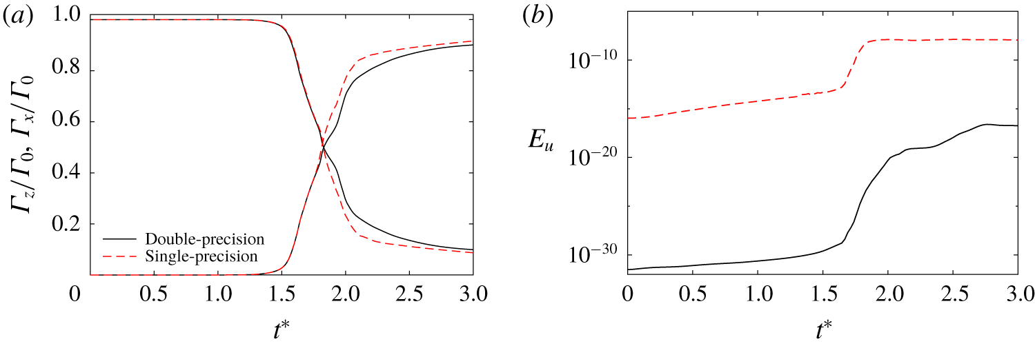
 $40\,000$ (see table 1 for details of the simulation parameters). To suppress and delay the symmetric breaking caused by the Kelvin–Helmholtz (planar jet) instability, double-precision arithmetic is employed. Appendix C presents a detailed comparison of full-domain simulations using single- and double-precision arithmetic at
 $Re=9000$, and demonstrates that the latter, which has smaller numerical round-off, can effectively suppress the occurrence of asymmetric structures. In addition, the symmetries of the initial condition ((2.9) and (2.10)) are further employed to subtract the anti-symmetric perturbations, which would otherwise inevitably grow for the planar jet. This two-fold symmetry, enabling us to simulate only a quarter of the domain, provides an additional benefit of being able to study the highly desirable, higher
 $Re$.
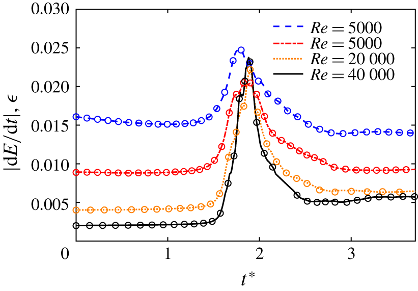
The rate of change of volume-integrated kinetic energy  $|\text{d}E/\text{d}t|$ (
 $\circ$ symbols) and energy dissipation
 $\unicode[STIX]{x1D716}$ (lines) as a function of the non-dimensionalized time
 $t^{\ast }=t/(2\unicode[STIX]{x03C0}b^{2}/\unicode[STIX]{x1D6E4}_{0})$ for different
 $Re$ values.

The adequacy of the numerical resolution is quantified by the rate of change of the volume-integrated kinetic energy  $E=\langle u_{i}^{2}/2\rangle$ (Archer, Thomas & Coleman Reference Archer, Thomas and Coleman2008; Van Rees et al. Reference Van Rees, Leonard, Pullin and Koumoutsakos2011), with the balance equation for flow in a triply periodic box being given as
 $$\begin{eqnarray}\displaystyle \frac{\text{d}E}{\text{d}t}=-\unicode[STIX]{x1D716}, & & \displaystyle\end{eqnarray}$$
where the kinetic energy dissipation  $\unicode[STIX]{x1D716}\equiv 2\unicode[STIX]{x1D708}\unicode[STIX]{x1D6FA}$, with
 $\unicode[STIX]{x1D6FA}=\langle \unicode[STIX]{x1D714}_{i}^{2}/2\rangle$ being the volume-integrated enstrophy. The difference between the left- and right-hand sides of equation (2.13) is a measure of the spatial discretization error. Figure 2 shows the time evolutions of
 $|\text{d}E/\text{d}t|$ and
 $\unicode[STIX]{x1D716}$ at four different Reynolds numbers. During the approaching phase, the dissipation is almost constant. However, when reconnection starts, vortex stretching results in the generation of finer scales, thus leading to a rapid increase of both enstrophy and dissipation. Even during this rapidly changing phase when the computational error could be expected to be large, the agreement between
 $|\text{d}E/\text{d}t|$ and
 $\unicode[STIX]{x1D716}$ is very good. For all the
 $Re$ considered, the maximum relative error between
 $|\text{d}E/\text{d}t|$ and
 $\unicode[STIX]{x1D716}$ is less than
 $1\,\%$.
Reynolds numbers and the associated numerical resolutions employed for the present simulations. The computational domain size is  $L_{y}\times L_{x}\times L_{z}=2\unicode[STIX]{x03C0}\times \unicode[STIX]{x03C0}\times \unicode[STIX]{x03C0}$.

3 Reconnection at  $Re=9000$

We first focus on  $Re=9000$, where the details of reconnection are more distinct and better visualized.
3.1 Flow visualization
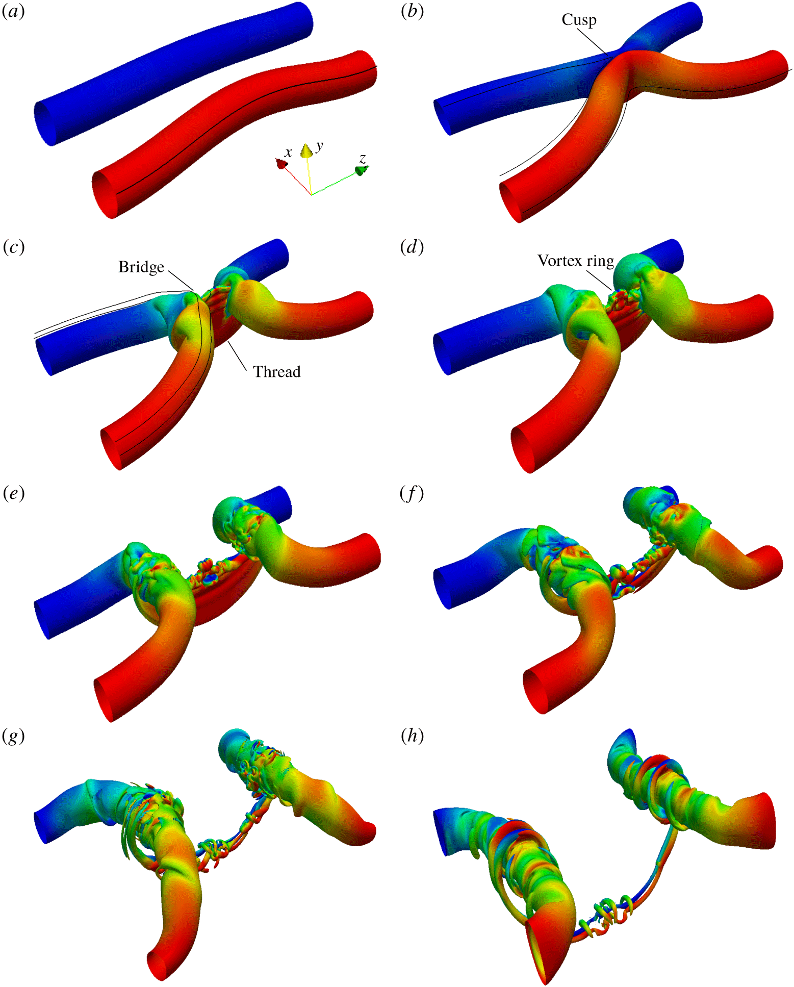
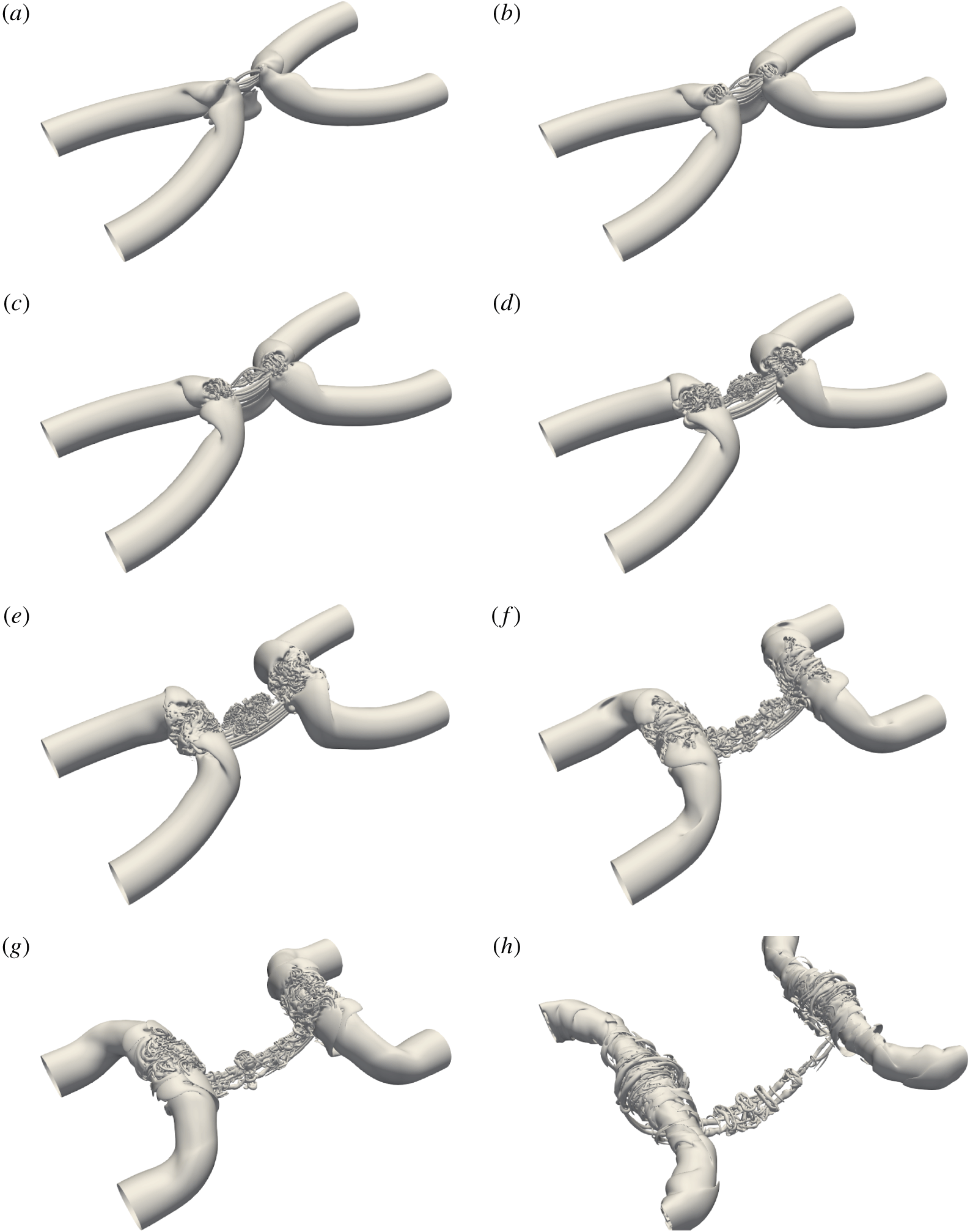
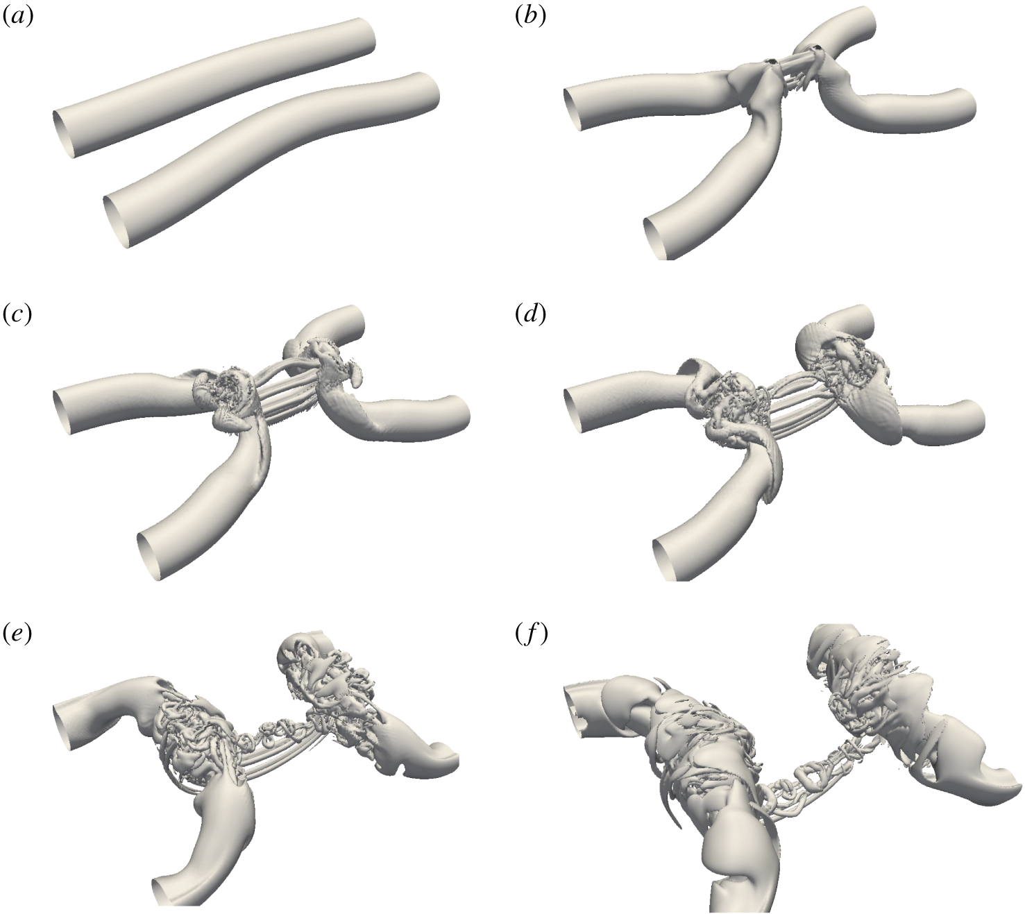
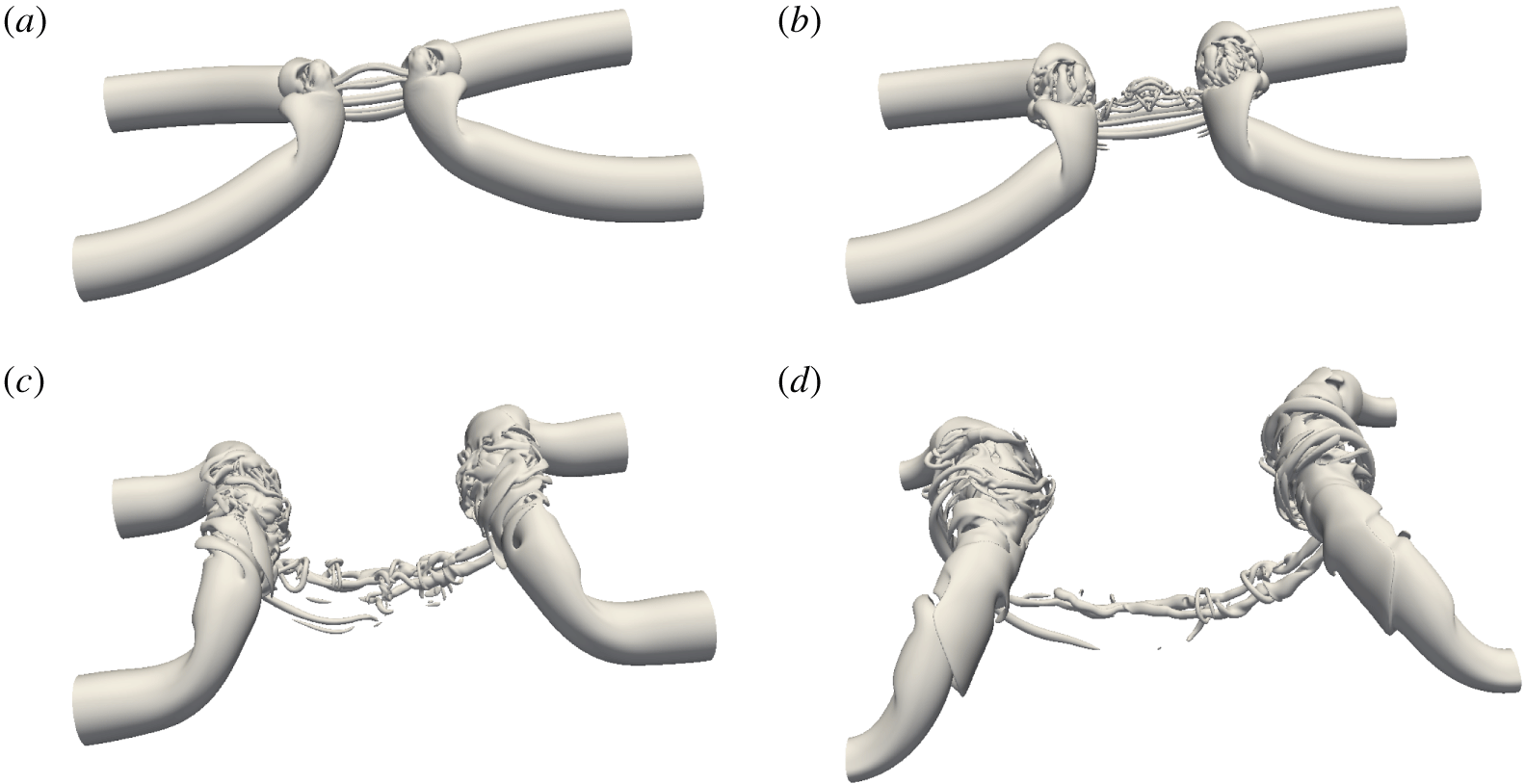
Figure 3 (and supplementary movie 1 available at https://doi.org/10.1017/jfm.2019.905) shows the time progression of the reconnection based on the vorticity magnitude isosurface  $|\unicode[STIX]{x1D74E}|$. Under self-induction, the curved vortex tubes approach each other and collide (figure 3b). Then viscosity acts to annihilate adjacent vorticity at the collision point. Thus, the closest vortex lines of opposite signs cut and connect, i.e. decimate both vorticities via cross-diffusion, to form two sharp cusps. These two cusps recede away from the plane of the colliding vortices by their curvature-driven self-induction; simultaneously, these cusped vortex lines are stretched out by the two initial vortices so that these cusps are removed as the lines are laid perpendicular to the original vortices (figure 3c). Successive reconnected vorticity lines are similarly laid on top of each other so that their accumulations form a transverse vortex (called a bridge). The remnant, unreconnected vortex lines continuously collide with each other and form two parallel thin sheet-like structures (called threads). In addition, the flow between the threads is similar to a planar jet. For the low-
 $Re$ cases (i.e.
 ${<}5000$), the curvature of the threads reverses due to the induced velocity of the two bridges causing the slowdown of the reconnection (MH). At this higher
 $Re=9000$, the bridges move apart rapidly so that the increased gap decreases the induced velocity between the two bridges, and hence is too weak to reverse the curvature of the threads. In addition, compared with the situation at low
 $Re$, the mutual induction between the stronger threads is enhanced. Hence, the threads easily overcome the thrust of the flow between the bridges.
Vorticity magnitude isosurfaces at 40 % of maximum initial vorticity (shaded with contours of axial vorticity) for  $Re=9000$: (a)
 $t^{\ast }=0$; (b)
 $t^{\ast }=1.51$; (c)
 $t^{\ast }=1.72$; (d)
 $t^{\ast }=1.92$; (e)
 $t^{\ast }=2.11$; (f)
 $t^{\ast }=2.34$; (g)
 $t^{\ast }=2.79$; (h)
 $t^{\ast }=3.70$. Lines in (a–c) represent the vortex lines. See also supplementary movie 1.

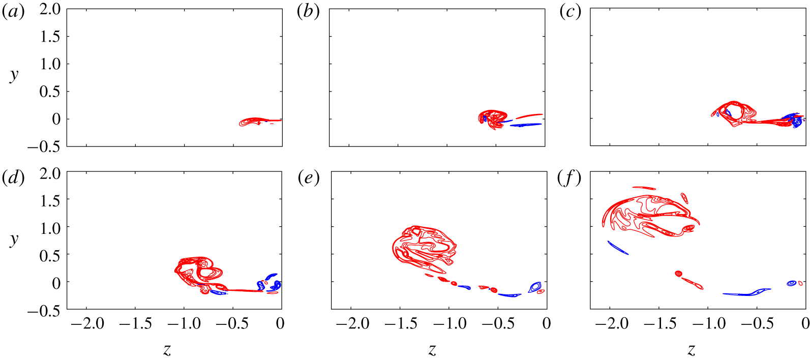
Mutual induction causes the peak vorticity regions of the threads to advect faster than the remainder, forming head–tail structures. As a result, a dipole forms at the top of the threads (see figure 3c; also see figure 8c for a better visualization with the vorticity isocontours in the symmetric plane). The adjacent parts of the elongated tails constitute a planar jet-like flow, which is very susceptible to a Kelvin–Helmholtz instability. For most previous moderate- $Re$ studies (van Rees et al. Reference van Rees, Hussain and Koumoutsakos2012; Beardsell et al. Reference Beardsell, Dufresne and Dumas2016, HD), this flow grows into rolls of anti-symmetric vortices (refer to figure 9 in HD as an example). Due to the imposition of symmetry here, only symmetric vortices grow as a series of vortex dipoles (figure 8d).
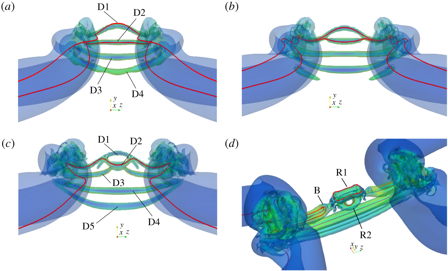
Close-up of the vortical structures based on the isosurfaces of  $\unicode[STIX]{x1D706}_{2}^{\ast }=-0.1$ during vortex ring formation: (a)
 $t^{\ast }=1.72$; (b)
 $t^{\ast }=1.77$; (c)
 $t^{\ast }=1.81$; (d)
 $t^{\ast }=1.86$. Note that D1–D5 denote the thread dipoles, R1 and R2 the newly formed vortex rings with B representing the associated bridgelets. The red lines in each panel are the vorticity lines.

Schematic illustration of the off-centre reconnection and vortex ring formation for the first two thread dipoles D1 and D2 in figure 4.

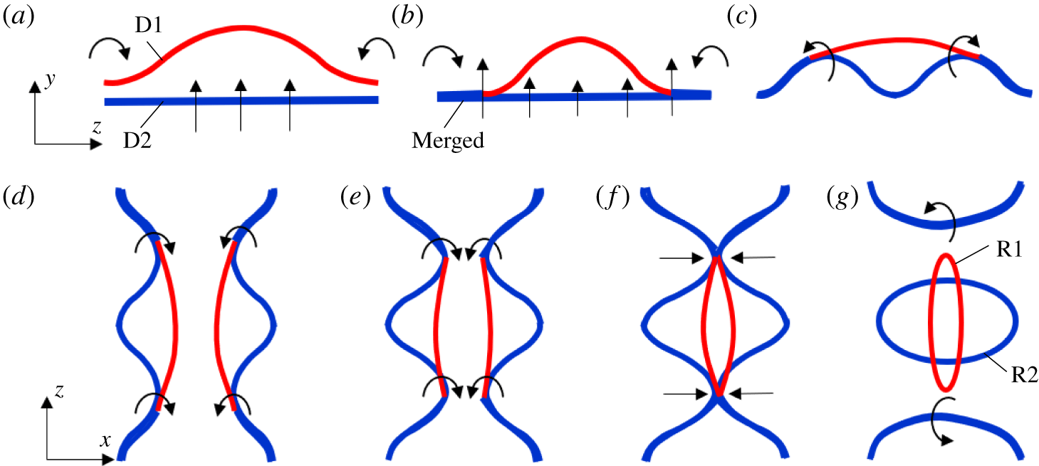
Then the top two vortex dipoles undergo reconnection and form two vortex rings (figure 3d). Such structures were also observed in Beardsell et al. (Reference Beardsell, Dufresne and Dumas2016) and McGavin & Pontin (Reference McGavin and Pontin2018). The generation of the vortex rings is a result of off-centre reconnections, which are now explained in detail in figure 4 and with adjoining illustrated sketches in figure 5. Note that due to the presence of strong shear in the interaction region, the  $\unicode[STIX]{x1D706}_{2}$ criterion (Jeong & Hussain Reference Jeong and Hussain1995) is employed in figure 4 for better visualizing the vortex structures. (The
 $\unicode[STIX]{x1D706}_{2}$ value is non-dimensionalized as
 $\unicode[STIX]{x1D706}_{2}^{\ast }=\unicode[STIX]{x1D706}_{2}/(\unicode[STIX]{x1D714}_{0}^{2}/4)$, where
 $\unicode[STIX]{x1D714}_{0}$ is the initial maximum vorticity.) Between the bridge dipole, there is a strong cross-flow in the
 $y$–
 $z$ plane – causing the thread to stretch and wrap around the bridges (figures 4a and 5a). As a consequence, the first thread dipole D1 then is pushed down and merges with the second one D2 near the bridge (indicated in figure 5b; also see vortex lines in figure 4b). Due to the fact that the induced velocity of the thread is proportional to the circulation (based on the Biot–Savart law), the merged part of the thread forms a stronger dipole pair near the bridges, and advects upward faster than the unmerged part near the centre. Under the combined effects of the advection of the bridges and the mutual induction of the thread dipole, the second dipole forms a double-humped wave (illustrated in figure 5c and also indicated by the vortex line in figure 4c). The merged top two thread dipoles then collide under curvature-induced self-induction and reconnect at the high curvature positions (illustrated in figure 5d–f). As a consequence, two elliptical vortex rings simultaneously form (denoted as R1 and R2 in figures 4d and 5g). Note that during this period, the third thread dipole also undergoes reconnection on the symmetric plane, whose bridgelets merged with the top one from the reconnection of the first two dipoles (denoted as B in figure 4d). The formation of vortex rings and their interaction with the remnant threads are found to be integral to the cascade scenario, especially for higher
 $Re$.
Isosurfaces of  $\unicode[STIX]{x1D706}_{2}^{\ast }=-0.1$ for
 $Re=9000$: (a)
 $t^{\ast }=1.92$; (b)
 $t^{\ast }=2.11$; (c)
 $t^{\ast }=2.34$; (d)
 $t^{\ast }=2.79$ (see also supplementary movie 2).

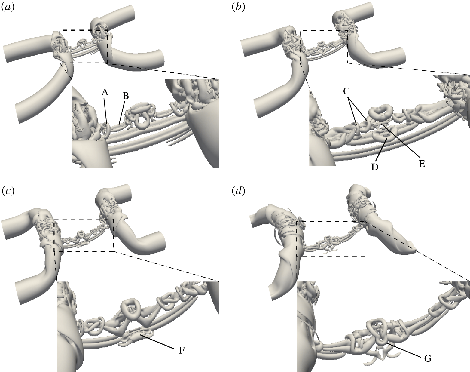
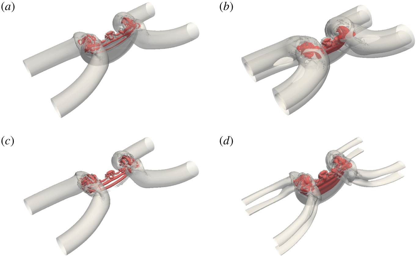
The secondary bridgelets rapidly move apart and merge with the main bridges (see A in figure 6a). Note that reconnection during the vortex ring formation is also incomplete, resulting in a finer thread dipole (B in figure 6a), which then diffuses out due to viscous effect. MH speculated that, at very high  $Re$, this secondary thread can further undergo higher generations of reconnection, forming a hierarchy of hairpin vortex packets. Due to the non-uniform curvature and the induced motion of thread dipoles, the two newly formed elliptical vortex rings undergo an oscillatory motion while advecting in the
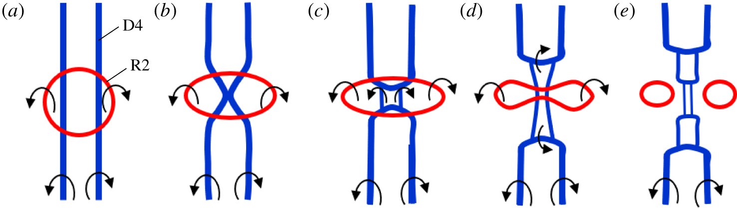
 $y$ direction, similar to those observed by Cheng, Lou & Lim (Reference Cheng, Lou and Lim2016), who studied the dynamics of a single elliptical vortex ring. The bottom ring R2 starts to interact with the thread dipole under it (figure 6b). The sequence is further illustrated in figure 7. In particular, the induced motion of bottom vortex ring R2 presses against the thread dipole D4 to reconnect (figure 7b–c). Subsequently, R2 also deforms and reconnects with D4 – generating two small side vortex rings and hairpin packet-like bridgelets (illustrated in figure 7d,e, and also indicated as C and D in figure 6b). Between the two hairpin packets, we also observe a finer-scale thread dipole (E in figure 6b). Note that the essence of the vortex reconnection cascade mechanism is well captured at this moment when three generations of vortices simultaneously exist – the primarily vortex tubes collide and reconnect, leaving the unreconnected parts as remnant threads, which further break up into secondary thread dipoles, and reconnect again, generating the third-level threads.
Schematic illustration of the interaction of vortex ring R2 and thread dipole D4, associated with figure 6(b).

As the bridges move further apart, the fifth thread dipole D5 (F in figure 6c) under mutual induction easily overcomes the thrust of the weakened jet between the bridges to reverse the curvature and reconnect. The reconnection process slowly stops when the threads become too weak to reverse their curvature (figures 3g and 6d). The remaining vortex ring R1 (G in figure 6d) is deformed under the induced motion of the thread dipole. At a late time (i.e.  $t^{\ast }=3.70$), only one clear thread dipole remains, and wraps around the bridges, similar to that observed at lower
 $Re$ (HD). However, due to the stretching of the thread dipole, several vortex filaments, which are orthogonal to the remnant thread, survive (figure 3h). In summary, the vortex reconnection at
 $Re=9000$ consists of successive reconnections, which clearly supports the reconnection cascade mechanism proposed by MH.
3.2 Vorticity in the symmetry planes and circulation transfer
Distributions of  $\unicode[STIX]{x1D714}_{z}$ in the symmetric plane at
 $Re=9000$: (a)
 $t^{\ast }=1.31$; (b)
 $t^{\ast }=1.51$; (c)
 $t^{\ast }=1.62$; (d)
 $t^{\ast }=1.72$; (e)
 $t^{\ast }=1.81$; (f)
 $t^{\ast }=1.92$; (g)
 $t^{\ast }=2.34$; (h)
 $t^{\ast }=2.79$. Positive and negative
 $z$-axis vorticity isocontours
 $|\unicode[STIX]{x1D714}_{z}|=[0.4\;0.6\;1\;2\;3\;5\;10\;15]$ of initial maximum vorticity are shown in red and blue, respectively. The curve in the right-hand part of each panel denotes
 $(\unicode[STIX]{x1D735}\times \unicode[STIX]{x1D74E})_{y}(0,y,0)$ normalized by its own maximum value along the intersecting line
 $\boldsymbol{l}$, illustrated in (a).

To better illustrate the reconnection process, we examine the vorticity distributions in the symmetric ( $S_{s}$) and collision (
 $S_{c}$) planes. The respective circulations in the two symmetry planes (
 $S_{s}$ and
 $S_{c}$) are defined as
 $$\begin{eqnarray}\displaystyle & \displaystyle \unicode[STIX]{x1D6E4}_{z}=\int _{S_{s}}\unicode[STIX]{x1D74E}\boldsymbol{\cdot }\boldsymbol{n}_{s}\,\text{d}S=\int _{-Lx/2}^{0}\int _{-Ly/2}^{Ly/2}\unicode[STIX]{x1D714}_{z}(x,y,0)\,\text{d}x\,\text{d}y, & \displaystyle\end{eqnarray}$$
 $$\begin{eqnarray}\displaystyle & \displaystyle \unicode[STIX]{x1D6E4}_{x}=\int _{S_{c}}\unicode[STIX]{x1D74E}\boldsymbol{\cdot }\boldsymbol{n}_{c}\,\text{d}S=\int _{-Lz/2}^{0}\int _{-Ly/2}^{Ly/2}\unicode[STIX]{x1D714}_{x}(0,y,z)\,\text{d}y\,\text{d}z, & \displaystyle\end{eqnarray}$$
where  $\boldsymbol{n}_{s}$ and
 $\boldsymbol{n}_{c}$ denote the unit vectors normal to the symmetric and collision planes.
During reconnection, circulation continuously transfers from  $S_{s}$ to
 $S_{c}$. Hence, the time variations of the circulations in these two planes are generally employed in previous studies to quantify the reconnection process, such as determining the reconnection time, the reconnection rate, etc. The rate of change of circulation in the symmetric plane
 $S_{s}$ is given by
 $$\begin{eqnarray}\displaystyle \frac{\unicode[STIX]{x2202}\unicode[STIX]{x1D6E4}_{z}}{\unicode[STIX]{x2202}t}=\frac{\unicode[STIX]{x2202}}{\unicode[STIX]{x2202}t}\int _{S_{s}}\unicode[STIX]{x1D74E}\boldsymbol{\cdot }\boldsymbol{n}_{\boldsymbol{s}}\,\text{d}S=\int _{S_{s}}\frac{\unicode[STIX]{x2202}\unicode[STIX]{x1D74E}}{\unicode[STIX]{x2202}t}\boldsymbol{\cdot }\boldsymbol{n}_{\boldsymbol{s}}\,\text{d}S. & & \displaystyle\end{eqnarray}$$
Substituting the vorticity equation (2.12) into (3.3), and applying the Stokes theorem, we further have (Stanaway, Shariff & Hussain Reference Stanaway, Shariff and Hussain1988)
 $$\begin{eqnarray}\displaystyle \frac{\unicode[STIX]{x2202}\unicode[STIX]{x1D6E4}_{z}}{\unicode[STIX]{x2202}t}=-\unicode[STIX]{x1D708}\oint _{\unicode[STIX]{x2202}S_{s}}(\unicode[STIX]{x1D735}\times \unicode[STIX]{x1D74E})\boldsymbol{\cdot }\text{d}\boldsymbol{l}=\unicode[STIX]{x1D708}\int _{-L_{y}/2}^{L_{y}/2}(\unicode[STIX]{x1D735}\times \unicode[STIX]{x1D74E})_{y}(0,y,0)\,\text{d}y, & & \displaystyle\end{eqnarray}$$
where  $\unicode[STIX]{x2202}S_{s}$ represents the boundary of half symmetric plane
 $S_{s}$ and
 $\boldsymbol{l}$ denotes the intersecting line of collision and symmetric planes (see figure 8a). Note that the second equality in (3.4) holds because
 $\unicode[STIX]{x1D735}\times \unicode[STIX]{x1D74E}$ is zero on three other sides of the rectangular loop
 $\unicode[STIX]{x2202}S_{s}$ besides
 $\boldsymbol{l}$. Hence, the total rate of circulation transferred from
 $S_{s}$ to
 $S_{c}$ can be measured by integrating
 $\unicode[STIX]{x1D708}(\unicode[STIX]{x1D735}\times \unicode[STIX]{x1D74E})_{y}$ along the intersecting line
 $\boldsymbol{l}$.
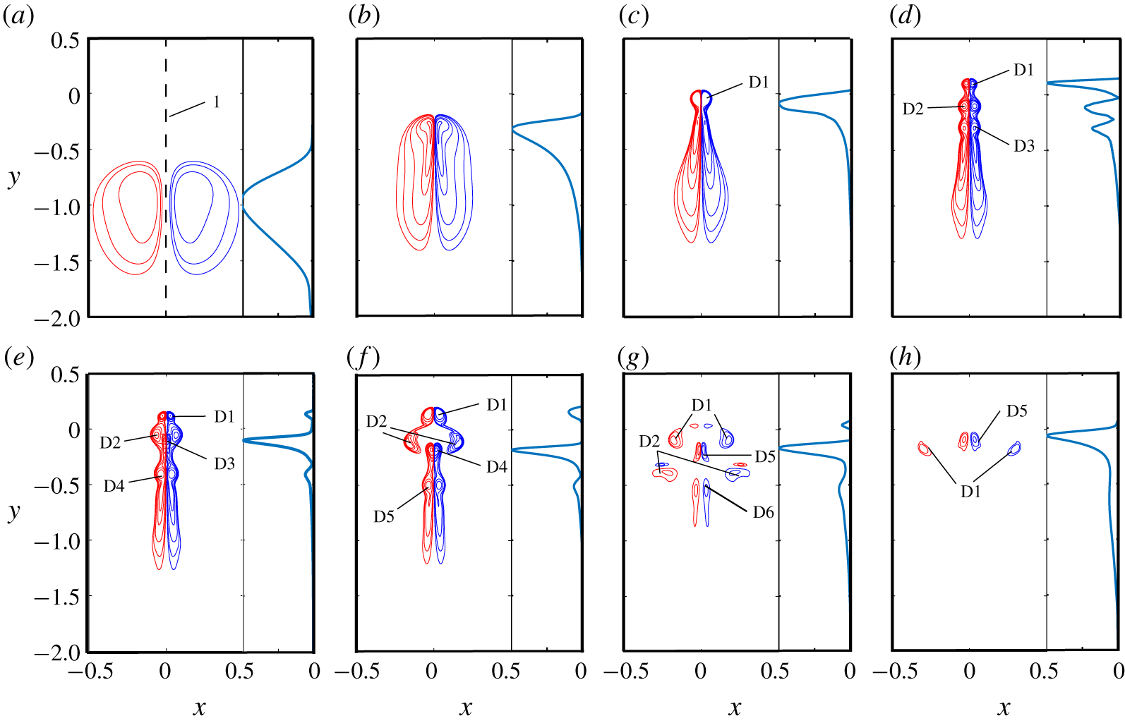
Figure 8 shows  $\unicode[STIX]{x1D714}_{z}$ distributions in the symmetric plane
 $S_{s}$ at different instants, along with the distribution of
 $(\unicode[STIX]{x1D735}\times \unicode[STIX]{x1D74E})_{y}$ along the intersecting line
 $\boldsymbol{l}$. The initially circular vortex tubes become elliptic as the peak vorticity regions mutually induce each other to advect faster than the other region, creating front–back asymmetry (figure 8a). By
 $t^{\ast }=1.51$ (figure 8b), the thread tubes approach each other via curvature-induced self-induction, hence forming the characteristic head–tail structures. The circulation transfer is relatively large near the head, where the vorticity gradient
 $\unicode[STIX]{x2202}\unicode[STIX]{x1D714}_{z}/\unicode[STIX]{x2202}x$ is large. The tail, however, also involves significant circulation transfer in spite of lower vorticity gradient, because of a large area. The heads with higher vorticity advect ahead of the tail due to mutual induction, forming a thread dipole at
 $t^{\ast }=1.62$ (denoted as D1 in figure 8c). The circulation of D1 is around
 $0.146$ of the initial circulation
 $\unicode[STIX]{x1D6E4}_{0}$ – correspondingly, the vortex Reynolds number
 $Re\approx 1300$. In the tail region in figure 8(c), the peak vorticity by mutual induction forms another dipole D2, leaving the remnant behind in the same scenario as the formation of D1. Similarly, the formation of D3 in figure 8(d). The circulations of D1, D2 and D3 at
 $t^{\ast }=1.72$ are approximately
 $0.058\unicode[STIX]{x1D6E4}_{0}$,
 $0.107\unicode[STIX]{x1D6E4}_{0}$ and
 $0.126\unicode[STIX]{x1D6E4}_{0}$, respectively, which correspond to
 $Re\approx 500$,
 $960$ and
 $1100$. Note that, compared with that at
 $t^{\ast }=1.62$,
 $60\,\%$ of the circulation is lost at
 $t^{\ast }=1.72$ for D1. The velocity induced by the bridges causes strong stretching of the thread dipoles, which intensifies the vorticity within the dipoles. In particular, at this time, the vorticity peaks for D1–D3 amplify to approximately
 $13$,
 $15$ and
 $11$ times the initial peak value
 $\unicode[STIX]{x1D714}_{0}$, respectively. In contrast to the low-
 $Re$ case, where the global vorticity peak typically locates in the symmetric plane
 $S_{s}$ (Brenner et al. Reference Brenner, Hormoz and Pumir2016), the global vorticity peak for our case (approximately
 $20\unicode[STIX]{x1D714}_{0}$) is not located on
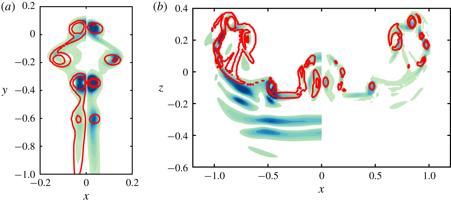
 $S_{s}$, which is caused by the off-centre reconnection discussed above.
As shown in figure 4, the first two dipoles evolve into two separate vortex rings, whose induced motions push D3 to collide and reconnect (figure 8e). Note that measuring circulation transfer between  $S_{s}$ and
 $S_{c}$ using
 $(\unicode[STIX]{x1D735}\times \unicode[STIX]{x1D74E})_{y}$ cannot capture the off-centre reconnection of forming vortex rings, where the circulation in each plane is unchanged. Hence, compared with the large values near the region of D3,
 $(\unicode[STIX]{x1D735}\times \unicode[STIX]{x1D74E})_{y}$ is relatively small around D1 and D2. As noted earlier, the elliptical vortex rings undergo oscillatory deformation, and the opposite ends of either elliptical vortex rings move apart in the symmetric plane
 $S_{s}$. They then approach and interact strongly with the fourth thread dipole D4 (figure 8f, and also figure 11c). At
 $t^{\ast }=2.34$ (figure 8g), the fourth dipole D4 is reconnected and disappeared in
 $S_{s}$. Besides, the vortex ring from the reconnection of D2 breaks up into two smaller vortex rings. As the main bridges further separate (figure 6c), the stretching of the threads by the two bridges weakens, and the vorticity magnitude decreases due to viscous diffusion. At
 $t^{\ast }=2.79$ (figure 8h), only D1 and D5 are strong enough to be visible – both D2 and D6 being weakened by cross-diffusion.
Contours of  $\unicode[STIX]{x1D714}_{x}$ in the collision plane at
 $Re=9000$: (a)
 $t^{\ast }=1.62$; (b)
 $t^{\ast }=1.72$; (c)
 $t^{\ast }=1.81$; (d)
 $t^{\ast }=1.92$; (e)
 $t^{\ast }=2.34$; (f)
 $t^{\ast }=2.79$. Positive and negative
 $z$-axis vorticity isocontours
 $|\unicode[STIX]{x1D714}_{z}|=[0.4~0.6~1~2~3~5~10~15]$ of initial maximum vorticity are shown in red and blue, respectively.

Figure 9 shows the corresponding contours of  $\unicode[STIX]{x1D714}_{x}$ in the collision plane
 $S_{c}$ (note that the contours before reconnection commences, i.e.
 $t^{\ast }<1.51$, are not shown). After reconnection, the bridges advect away from the reconnected region due to self-induced motion (figure 9a). In addition, the newly reconnected small bridgelets continuously pair and merge with the main bridges, this being associated with the inverse energy cascade discussed later. Figure 9(c) shows that the bridges have relatively strong vorticity with non-concentric distributions, which play an important role in the bridges’ internal dynamics. In regions where
 $|\unicode[STIX]{x1D74E}|$ is larger, the vortex filaments rotate fast thereby leading to the overall twisting of vortex lines in the bridge. In turn, twisted vortex lines produce axial flow along the vortex (Virk, Hussain & Kerr Reference Virk, Hussain and Kerr1995), which further introduce deformation and oscillation of the vortex core – known as core dynamics (Melander & Hussain Reference Melander and Hussain1994). It is interesting to observe that there exists opposite-signed vorticity in the bridges, which disappears in the later times due to cross-diffusion, e.g. at
 $t^{\ast }=1.92$ in figure 9(d). This finding is consistent with the so-called ‘internal reconnection’ in the bridges observed by McGavin & Pontin (Reference McGavin and Pontin2018). At
 $t^{\ast }=2.34$ (figure 9e), the vorticity in the bridges becomes more concentric due to viscous diffusion. Between the main bridges, there are multiple vorticity patches, each corresponding to a head of hairpin-like bridgelets.
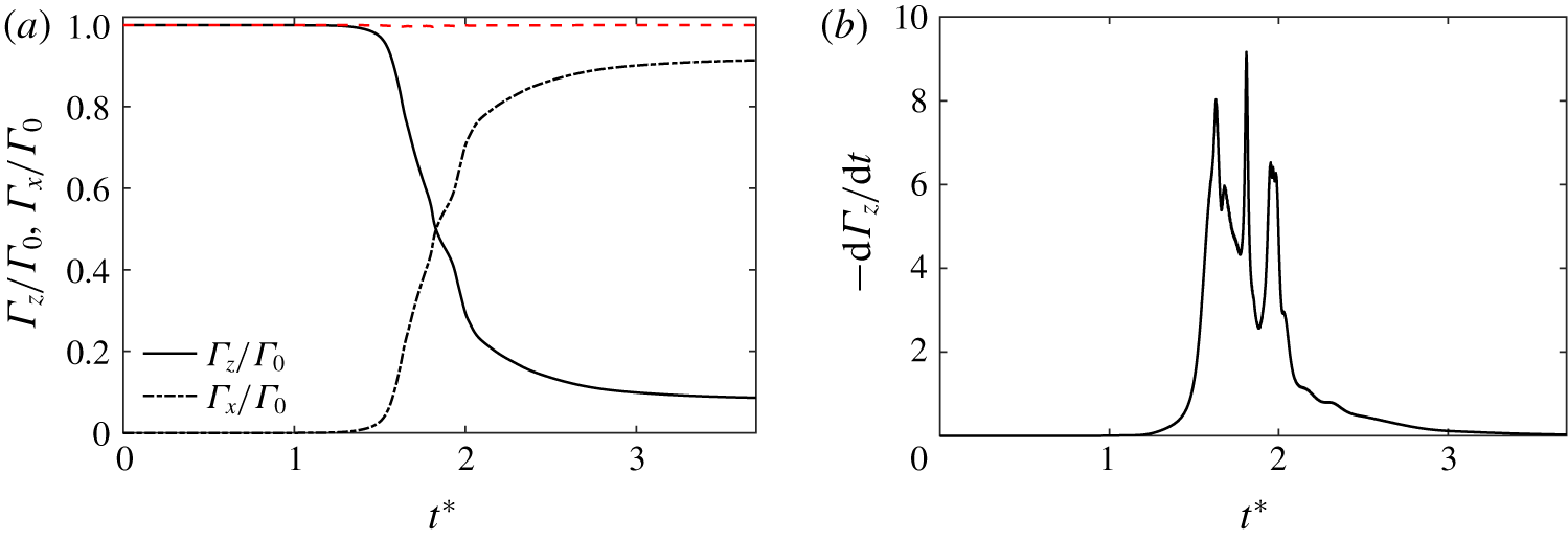
Time evolution of (a) circulation  $\unicode[STIX]{x1D6E4}_{x}$ and
 $\unicode[STIX]{x1D6E4}_{z}$ and (b) circulation transfer rate
 $-\unicode[STIX]{x2202}\unicode[STIX]{x1D6E4}_{z}/\unicode[STIX]{x2202}t$ at
 $Re=9000$. Note that the dashed line in (a) indicates the sum of
 $\unicode[STIX]{x1D6E4}_{x}$ and
 $\unicode[STIX]{x1D6E4}_{z}$.

Figure 10(a) shows the time evolution of  $\unicode[STIX]{x1D6E4}_{z}$ and
 $\unicode[STIX]{x1D6E4}_{x}$ for
 $Re=9000$, along with figure 10(b) showing the corresponding circulation transfer rate
 $-\unicode[STIX]{x2202}\unicode[STIX]{x1D6E4}_{z}/\unicode[STIX]{x2202}t$. Note that the sum of the circulations in the two half-planes (
 $\unicode[STIX]{x1D6E4}_{x}+\unicode[STIX]{x1D6E4}_{z}$) remains constant in figure 10(a) – as expected by Kelvin’s theorem – which is a good indication of the accuracy of the numerics. During the approach phase,
 $\unicode[STIX]{x1D6E4}_{z}$ is nearly unchanged. Due to the reconnection process, a sudden drop in
 $\unicode[STIX]{x1D6E4}_{z}$ occurs at
 $t^{\ast }=1.5$ with a corresponding increase in
 $\unicode[STIX]{x1D6E4}_{x}$. It is interesting that
 $\unicode[STIX]{x1D6E4}_{x}$ and
 $\unicode[STIX]{x1D6E4}_{z}$ variations are not really smooth – the circulation transfer rate
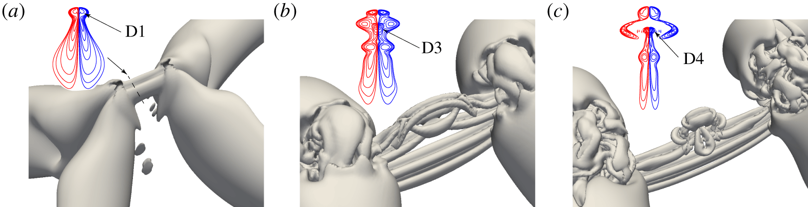
 $-\unicode[STIX]{x2202}\unicode[STIX]{x1D6E4}_{z}/\unicode[STIX]{x2202}t$ contains three distinct peaks, indicating that reconnection is not a continuous process, as to be expected because the vorticity sheets formed by collision break into vortex dipoles as explained earlier. The vortical structures at these peaks are shown in figure 11. The first peak develops at
 $t^{\ast }=1.62$ when the first dipole D1 forms and the associated cross-diffusion is strong. The second peak occurs at
 $t^{\ast }=1.81$, resulting from the reconnection of third thread dipole D3 (marked in figure 11b). As discussed above, the off-centre reconnections of the first two dipoles D1 and D2 leading to the formation of vortex rings have no effect on the circulation variation, because a cut through vortex ring contributes zero net circulation as opposite circulations cancel each other. The third peak forms at
 $t^{\ast }=1.96$, which is related to the reconnection of the fourth thread dipole D4 under the influence of vortex ring R2 (figure 11c). It is also interesting that
 $-\unicode[STIX]{x2202}\unicode[STIX]{x1D6E4}_{z}/\unicode[STIX]{x2202}t$ changes more abruptly before initiation of reconnection than at its end, the latter being contributed by slower cross-diffusion by the tails. For
 $t^{\ast }\geqslant 2.7$,
 $-\unicode[STIX]{x2202}\unicode[STIX]{x1D6E4}_{z}/\unicode[STIX]{x2202}t$ approaches zero – indicating the slow stop of reconnection.
Vortical structures visualized with  $\unicode[STIX]{x1D706}_{2}^{\ast }=-0.1$, along with
 $\unicode[STIX]{x1D714}_{z}$ contours in the symmetric plane indicated as a dashed line in (a), at the time of peak circulation transfer at
 $Re=9000$: (a)
 $t^{\ast }=1.62$; (b)
 $t^{\ast }=1.81$; (c)
 $t^{\ast }=1.96$.

3.3 Separation distance
A particularly interesting question for reconnection is the separation distance between the two initial approaching vortex tubes, as well as the separation of the resulting bridges. The acceleration of vortices is found to play a significant role in noise generation (Möhring Reference Möhring1978; Kambe & Minota Reference Kambe and Minota1981; Howe Reference Howe2003). Assuming that a reconnection event is a local process in space, and the circulation  $\unicode[STIX]{x1D6E4}$ is the only relevant dimensional quantity involved, simple dimensional analysis suggests that the distance
 $\unicode[STIX]{x1D6FF}(t)$ between two vortex filaments should scale as
 $$\begin{eqnarray}\displaystyle \unicode[STIX]{x1D6FF}(t)\sim (\unicode[STIX]{x1D6E4}t)^{1/2}. & & \displaystyle\end{eqnarray}$$
Such a prediction has been confirmed by numerous studies, such as the reconnection for viscous filaments (Kimura & Moffatt Reference Kimura and Moffatt2018) and in superfluids (Baggaley et al. Reference Baggaley, Sherwin, Barenghi and Sergeev2012; Villois, Proment & Krstulovic Reference Villois, Proment and Krstulovic2017; Fonda et al. Reference Fonda, Sreenivasan and Lathrop2019). Note that several numerical studies for quantum reconnection, such as those of Zuccher et al. (Reference Zuccher, Caliari, Baggaley and Barenghi2012) and Rorai et al. (Reference Rorai, Skipper, Kerr and Sreenivasan2016), reported deviations from the  $1/2$ scaling; however, we do not address this issue here.
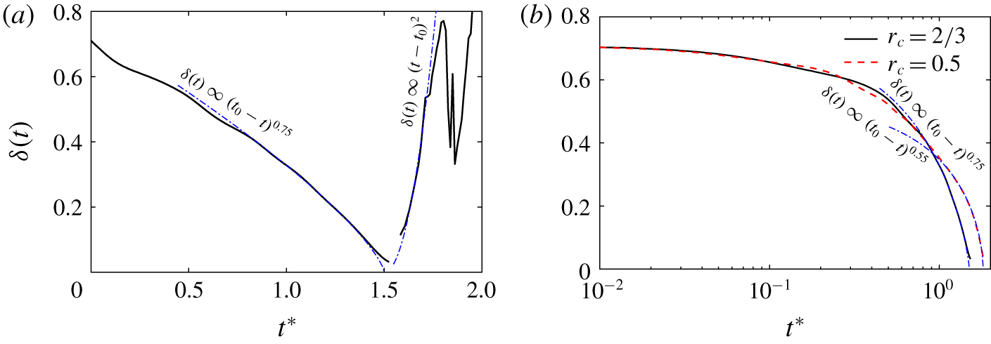
(a) Time evolution of separation distance; (b) separation distance before first reconnection for different core size at  $Re=9000$. Note that the dot-dashed lines correspond to
 $-0.75$ and
 $-0.55$ for
 $r_{c}=2/3$ and 0.5, respectively.

Unlike superfluid or vortex filament reconnections, where each reconnection is complete with no thread, the separation distance  $\unicode[STIX]{x1D6FF}(t)$ during viscous vortex reconnection cannot be sharply defined. Before the reconnection event, the tubes undergo significant core deformation; during reconnection, the reconnected vortex filaments take some time to collect together to form the bridge. In both stages, the vorticity is distributed in irregular shapes without any clear vortex centre. Following HD, we take the vorticity centroid (computed as the centroid of all vorticity which is above 75 % of the maximum vorticity) to be the centre of the tubes and bridges. Figure 12(a) shows the time evolution of separation distances before and after reconnection. This distance is found to scale as
 $(t_{0}-t)^{3/4}$ before reconnection, which is consistent with the finding of HD. Here,
 $t_{0}\approx 1.5$ is the time when the centres are the closest. This scaling is quite different from that reported for quantum and viscous filament reconnections. The disagreement is likely due to the failure of the local assumption that the core size and shape do not affect the approaching speed. To confirm this, we conduct an additional simulation with the same configuration at
 $Re=9000$ but with a smaller core radius (i.e.
 $r_{c}=0.5$ as opposed to
 $r_{c}=2/3$ used in the rest of the paper) so that the core size effect can be reduced. Interestingly, the scaling for
 $r_{c}=0.5$ is reduced to approximately
 $(t_{0}-t)^{0.55}$ (figure 12b), which is very close to the
 $1/2$ scaling observed for superfluid and viscous filament reconnections. Reconnected vortex lines first form sharp cusps and retract rapidly away from the reconnection site. Due to the high curvature, the repulsion is hence much faster than the collision. Consistent with HD, the separation distance after reconnection is found to scale as
 $(t-t_{0})^{2}$ – distinct from quantum vortex reconnection, where the repulsion after reconnection also scales as
 $(t-t_{0})^{1/2}$ (Fonda et al. Reference Fonda, Sreenivasan and Lathrop2019).
3.4 Energy cascade
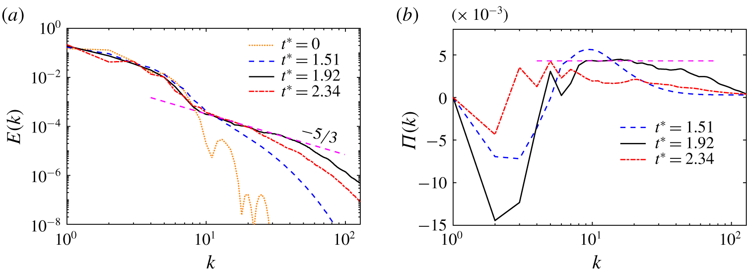
(a) Kinetic energy spectrum  $E(k)$ and (b) the corresponding energy flux spectrum
 $\unicode[STIX]{x1D6F1}(k)$ for several instants at
 $Re=9000$. The dashed line in (a) indicates the
 $-5/3$ slope; and the dashed line in (b) is an arbitrary line only as a reference.

Turbulent flows are often viewed as a hierarchy of eddies with different scales or a tangle of vortices. It still remains an open question as to how the energy cascades through different scales. Most studies have looked at turbulence energy cascade from either the spectral or physical perspective. From the spectral perspective, the energy cascade is understood as the interaction between adjacent wavenumbers (Obukhov Reference Obukhov1941; Domaradzki & Carati Reference Domaradzki and Carati2007). From the spatial perspective, energy transfer across different scales is often assumed to be due to vortex stretching, in which vortical structures of a given scale are stretched and intensified by larger vortices (Taylor & Green Reference Taylor and Green1937; Goto Reference Goto2008; Mao & Hussain Reference Mao and Hussain2017; Doan et al. Reference Doan, Swaminathan, Davidson and Tanahashi2018). However, the link between these two approaches is still unclear. Here we explore if viscous vortex reconnection can serve as a physical mechanism capturing the details of energy cascade. The balance equation for the energy spectrum  $E(k,t)$ is
 $$\begin{eqnarray}\displaystyle \frac{\unicode[STIX]{x2202}}{\unicode[STIX]{x2202}t}E(k,t)=P(k,t)+T(k)-2\unicode[STIX]{x1D708}k^{2}E(k,t), & & \displaystyle\end{eqnarray}$$
where the three terms on the right-hand side represent energy injection (via external forcing), energy transfer and dissipation, respectively (Frisch Reference Frisch1995). For the reconnection case considered here,  $P(k,t)$ is absent as there is no external forcing.
Figure 13(a) shows the energy spectrum  $E(k,t)$ during viscous reconnection at various instants for
 $Re=9000$. At
 $t^{\ast }=0$, most energy is concentrated at small wavenumbers, corresponding to the length scales of the initial vortex tubes. The power-law regime at large wavenumbers is manifested as soon as the tubes first touch at
 $t^{\ast }\approx 1.51$. At
 $t^{\ast }=1.92$, we observe a large increase in the small-scale energy as expected from the concept of cascade, and the spectrum develops a distinct power law with
 $-5/3$ slope. Note that
 $t^{\ast }=1.92$ roughly corresponds to the time of the maximum of volume-integrated enstrophy
 $\unicode[STIX]{x1D6FA}$. To capture vortical structures in different scales, the full flow field is filtered with a sharp bandpass filter:
 $$\begin{eqnarray}\displaystyle \widehat{\unicode[STIX]{x1D74E}}^{(c)}(\boldsymbol{k})=\left\{\begin{array}{@{}ll@{}}\widehat{\unicode[STIX]{x1D74E}}(\boldsymbol{k}),\quad & \text{if }k_{l}<|\boldsymbol{k}|<k_{h};\\ 0,\quad & \text{otherwise},\end{array}\right. & & \displaystyle\end{eqnarray}$$
where  $k_{l}$ and
 $k_{h}$ are the lower and upper bounds of the cutoff wavenumbers. Then a bandpass-filtered vorticity field
 $\unicode[STIX]{x1D74E}^{(c)}$ is obtained by applying inverse Fourier transform to the filtered field
 $\widehat{\unicode[STIX]{x1D74E}}^{(c)}(\boldsymbol{k})$.
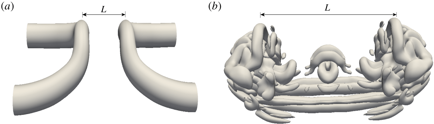
Band-filtered vortical structures in the large-scale range ( $k\leqslant 7$) and inertial range (
 $10\leqslant k\leqslant 40$) are visualized in figures 14(a) and 14(b), respectively. The structures in the large-scale range correspond to the reconnected main bridges, and those in the inertial range are the stretched threads, vortex rings and reconnected small-scale bridgelets. It clearly suggests that vortex reconnection is an important physical mechanism for Kolmogorov energy cascade. In addition to vortex reconnection, the vortex stretching associated with reconnection is also essential for the energy cascade. Under the strong strain field induced by the bridges, the threads are continuously stretched to generate smaller-scale dipoles, shown in figure 6(a–c). The vortex stretching mechanism presented here is closely related to the cascade scenarios found in other types of flows, such as vortex–turbulence interaction (Melander & Hussain Reference Melander and Hussain1993) and homogeneous isotropic turbulence (Goto Reference Goto2008). Note that our reconnection cascade scenario is different from Kerr (Reference Kerr2013b), who studied vortex reconnection of two long, straight anti-parallel vortex tubes with localized bumps – the long tubes undergo successive reconnections due to the propagation of the Kelvin waves; and these reconnections lead to the formation of swirling vortex rings, which then break up into turbulence, giving rise to a
 $-5/3$ spectrum. At later times (i.e.
 $t^{\ast }=2.34$), the energy in the high wavenumbers gradually decays by dissipation. The slope of power-law regimes is gradually reduced.
Band-filtered vortical structures in the (a) large-scale range ( $k\leqslant 7$) and (b) inertial range (
 $10\leqslant k\leqslant 40$) visualized by the isosurface of
 $\unicode[STIX]{x1D706}_{2}^{\ast }=-0.1$ at
 $t^{\ast }=1.92$ for
 $Re=9000$. The lines denote the centre-to-centre distance between the two bridges.

Figure 13(b) further shows the energy flux spectra  $\unicode[STIX]{x1D6F1}(k)=\int _{k}^{\infty }T(k^{\prime })\,\text{d}k^{\prime }$ at various times, where
 $T(k)$ is the energy transfer in equation (3.6). The
 $\unicode[STIX]{x1D6F1}(k)$ spectrum exhibits two different regions. First, positive values at high wavenumbers reflect the energy transfer to small scales. On the other hand, the negative values at small wavenumbers suggest an inverse cascade, which might be related to the merger process of bridges, evidenced in figure 9. As also found in the homogeneous isotropic turbulence, a plateau is observed in the energy flux in the inertial range at
 $t^{\ast }=1.92$, when a distinct
 $-5/3$ energy spectrum forms. The energy transfer rate between different scales progressively slows down at the late stage of the reconnection (for example,
 $t^{\ast }=2.34$).
One important aspect in classical turbulent energy cascade is the locality of interactions between different scales (Taylor & Green Reference Taylor and Green1937; Domaradzki & Rogallo Reference Domaradzki and Rogallo1990). From the physical space perspective, it suggests that a vortex of a given size is stretched primarily by the strain from structures that are three to five times larger (Leung, Swaminathan & Davidson Reference Leung, Swaminathan and Davidson2012; Doan et al. Reference Doan, Swaminathan, Davidson and Tanahashi2018). It is therefore appropriate to investigate the scale locality in vortex reconnection. The scale-by-scale transfer and interaction is analysed by following the method proposed by Davidson, Morishita & Kaneda (Reference Davidson, Morishita and Kaneda2008) (see also Doan et al. (Reference Doan, Swaminathan, Davidson and Tanahashi2018)) – summarized as follows. The velocity  $\boldsymbol{u}$ and vorticity
 $\unicode[STIX]{x1D74E}$ are decomposed into large and small scales such that
 $\boldsymbol{u}=\boldsymbol{u}^{L}+\boldsymbol{u}^{S}$ and
 $\unicode[STIX]{x1D74E}=\unicode[STIX]{x1D74E}^{L}+\unicode[STIX]{x1D74E}^{S}$, where the superscripts
 $L$ and
 $S$ respectively denote the larger and smaller structures compared to a selected scale.
Since the physical mechanism of enstrophy cascade from large to small scales is the same as for energy cascade (Doan et al. Reference Doan, Swaminathan, Davidson and Tanahashi2018), here only the enstrophy cascade is investigated. The enstrophy equations for the large and small structures can be obtained by taking the dot product of  $\unicode[STIX]{x1D74E}^{L}$ or
 $\unicode[STIX]{x1D74E}^{S}$ with the vorticity equation (2.12):
 $$\begin{eqnarray}\displaystyle & \displaystyle \frac{\unicode[STIX]{x2202}}{\unicode[STIX]{x2202}t}\langle (\unicode[STIX]{x1D74E}^{L})^{2}/2\rangle =-F(r)+G^{L}(r)-\unicode[STIX]{x1D708}\langle (\unicode[STIX]{x1D735}\times \unicode[STIX]{x1D74E}^{L})^{2}\rangle , & \displaystyle\end{eqnarray}$$
 $$\begin{eqnarray}\displaystyle & \displaystyle \frac{\unicode[STIX]{x2202}}{\unicode[STIX]{x2202}t}\langle (\unicode[STIX]{x1D74E}^{S})^{2}/2\rangle =F(r)+G^{S}(r)-\unicode[STIX]{x1D708}\langle (\unicode[STIX]{x1D735}\times \unicode[STIX]{x1D74E}^{S})^{2}\rangle , & \displaystyle\end{eqnarray}$$
where  $F(r)=\langle \unicode[STIX]{x1D74E}^{L}\boldsymbol{\cdot }(\boldsymbol{u}\boldsymbol{\cdot }\unicode[STIX]{x1D735}\unicode[STIX]{x1D74E}^{S})\rangle =-\langle \unicode[STIX]{x1D74E}^{S}\boldsymbol{\cdot }(\boldsymbol{u}\boldsymbol{\cdot }\unicode[STIX]{x1D735}\unicode[STIX]{x1D74E}^{L})\rangle$ is the enstrophy flux from large to small scales across the scale
 $r$, and
 $G^{L}(r)=\langle \unicode[STIX]{x1D74E}^{L}\boldsymbol{\cdot }(\unicode[STIX]{x1D74E}\boldsymbol{\cdot }\unicode[STIX]{x1D735}\boldsymbol{u})\rangle$ and
 $G^{S}(r)=\langle \unicode[STIX]{x1D74E}^{S}\boldsymbol{\cdot }(\unicode[STIX]{x1D74E}\boldsymbol{\cdot }\unicode[STIX]{x1D735}\boldsymbol{u})\rangle$ represent the generation of enstrophy via vortex stretching at large and small scales, respectively. From this formalism, the transfer of enstrophy from scale
 $L$ to
 $S$ across the scale
 $r$ can be analysed by studying the enstrophy flux
 $F$.
The spectral space bandpass filtering procedure is employed to educe the structure of a given length scale  $L$:
 $$\begin{eqnarray}\displaystyle \widehat{\boldsymbol{u}}^{L}(\boldsymbol{k})=\frac{\unicode[STIX]{x1D6FC}}{\sqrt{L}}2\unicode[STIX]{x1D705}^{2}e^{-\unicode[STIX]{x1D705}^{2}}\widehat{\boldsymbol{u}}(\boldsymbol{k}), & & \displaystyle\end{eqnarray}$$
where  $\unicode[STIX]{x1D705}=kL/2$ with
 $k=|\boldsymbol{k}|$, and
 $\unicode[STIX]{x1D6FC}=\sqrt{2}$. Then the bandpass-filtered velocities at some specified large and small scales
 $L$ and
 $S$ can be used to directly compute enstrophy transfer
 $F^{L\rightarrow S}$ from scales
 $L$ to
 $S$:
 $$\begin{eqnarray}\displaystyle F^{L\rightarrow S}=\langle \unicode[STIX]{x1D74E}^{L}\boldsymbol{\cdot }(\boldsymbol{u}\boldsymbol{\cdot }\unicode[STIX]{x1D735}\unicode[STIX]{x1D74E}^{S})\rangle . & & \displaystyle\end{eqnarray}$$
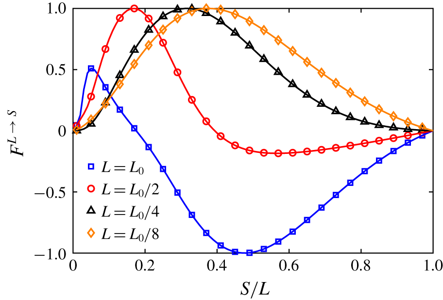
Figure 15 shows the normalized enstropy flux  $\overline{F}^{L\rightarrow S}=F^{L\rightarrow S}/\max (|F^{L\rightarrow S}|)$ as a function of
 $S/L$ at
 $t^{\ast }=1.92$ for different choices of the large scales
 $L=L_{0}$,
 $L_{0}/2$,
 $L_{0}/4$ and
 $L_{0}/8$. Here
 $L_{0}$ is chosen such that the bandpass-filtered energy spectrum is peaked around
 $k_{0}=3$ (near the negative peak in figure 13b). For a given large scale
 $L$, the small scale
 $S$ is varied to determine which small scale receives/sends the most energy from/to the structures of size
 $L$. When
 $L=L_{0}$, enstropy is mostly inverse-transferred from small scales to the large scale, with a peak around
 $S/L=0.5$. This is consistent with the inverse energy cascade observed in the energy flux spectrum (figure 13b). In addition, there is also a small positive peak around
 $S/L=0.2$, implying a small portion of forward enstrophy transfer to the small scales. As large scale
 $L$ decreases, the enstrophy cascade becomes purely forward to small scales. In particular, the enstrophy is mostly transferred to scales of about
 $0.3L$, when the large scale is located in the inertia range (i.e.
 $L=L_{0}/4$). This is consistent with the finding of Doan et al. (Reference Doan, Swaminathan, Davidson and Tanahashi2018) for homogeneous isotropic turbulence and confirms the existence of scale locality in energy/enstropy transfer.
Normalized enstrophy flux  $\overline{F}^{L\rightarrow S}$ at
 $t^{\ast }=1.92$ for
 $Re=9000$. Here
 $L_{0}$ is selected so that the bandpass-filtered energy spectrum is peaked around
 $k_{0}=3$.

Prompted by one of the referees, we also examined the nature and significance of vortex sheet-like structures. When visualized using the  $\unicode[STIX]{x1D706}_{2}$ criterion, our analysis of energy cascade is mainly focused on the vortex tube-like structures in which vorticity dominates. In turbulence, both vortex tubes and sheets are considered as the structural building blocks of energy cascade (Bermejo-Moreno, Pullin & Horiuti Reference Bermejo-Moreno, Pullin and Horiuti2009; Wu Reference Wu2017). Hence, vortex sheet-like structures might also be important for further elucidating energy cascade and dissipation. For extracting the vortex sheet-like structures, we adopt the method proposed by Horiuti & Takagi (Reference Horiuti and Takagi2005). The eigenvalues of the symmetric second-order tensor
 $\unicode[STIX]{x1D608}_{ij}\equiv \unicode[STIX]{x1D61A}_{ik}\unicode[STIX]{x1D6FA}_{kj}+\unicode[STIX]{x1D61A}_{jk}\unicode[STIX]{x1D6FA}_{ki}$ are reordered as
 $[\unicode[STIX]{x1D608}_{ij}]_{\unicode[STIX]{x1D714}}$,
 $[\unicode[STIX]{x1D608}_{ij}]_{+}$ and
 $[\unicode[STIX]{x1D608}_{ij}]_{-}$, with
 $[\unicode[STIX]{x1D608}_{ij}]_{\unicode[STIX]{x1D714}}$ being the eigenvalue whose corresponding eigenvector is most aligned with the vorticity vector, and
 $[\unicode[STIX]{x1D608}_{ij}]_{+}$ and
 $[\unicode[STIX]{x1D608}_{ij}]_{-}$ are the remaining larger and smaller eigenvalues. Based on the feature of vortex sheets, in which both strain rate and vorticity are large and correlated,
 $[\unicode[STIX]{x1D608}_{ij}]_{+}$ was demonstrated by Horiuti & Takagi (Reference Horiuti and Takagi2005) to be a good metric for identifying vortex sheet-like structures.
For better understanding energy cascade and dissipation, and also their relationship with vortex tube- and sheet-like structures, we show in figure 16 the educed structures of local enstrophy  $\unicode[STIX]{x1D714}_{i}\unicode[STIX]{x1D714}_{i}$, dissipation rate
 $\unicode[STIX]{x1D61A}_{ij}\unicode[STIX]{x1D61A}_{ij}$,
 $\unicode[STIX]{x1D706}_{2}$ and
 $[\unicode[STIX]{x1D608}_{ij}]_{+}$. Let us first consider the original vortical structure away from the reconnecting region. The enstrophy structures are predominantly tube-like with dissipation structures at their periphery (where the strain rate is maximized), akin to the typical Burgers-like vortex model. As expected,
 $\unicode[STIX]{x1D706}_{2}$ also captures the tube-like structures, akin to the enstrophy structures. As the two vortex tubes advect upward due to mutual induction, the initial circular vortex deforms into an elliptical shape, and, interestingly,
 $[\unicode[STIX]{x1D608}_{ij}]_{+}$ identifies the ends of the elliptic vortex as ‘vortex sheets’. In the interaction region, when using low thresholds,
 $\unicode[STIX]{x1D714}_{i}\unicode[STIX]{x1D714}_{i}$,
 $\unicode[STIX]{x1D61A}_{ij}\unicode[STIX]{x1D61A}_{ij}$ and
 $[\unicode[STIX]{x1D608}_{ij}]_{+}$ all can capture the vortex sheet structures, while
 $\unicode[STIX]{x1D706}_{2}$ captures tube-like structures. When using a higher threshold,
 $\unicode[STIX]{x1D714}_{i}\unicode[STIX]{x1D714}_{i}$ structure closely resembles the tube-like structures induced with
 $\unicode[STIX]{x1D706}_{2}$. But
 $[\unicode[STIX]{x1D608}_{ij}]_{+}$ still remains predominantly sheet-like, confirming the relevance of sheet-like structures not only in turbulent flows but also in vortex interactions.
Three-dimensional structures of (a)  $\unicode[STIX]{x1D714}_{i}\unicode[STIX]{x1D714}_{i}$, (b)
 $\unicode[STIX]{x1D61A}_{ij}\unicode[STIX]{x1D61A}_{ij}$, (c)
 $\unicode[STIX]{x1D706}_{2}$ and (d)
 $[\unicode[STIX]{x1D608}_{ij}]_{+}$ at
 $t^{\ast }=1.92$ for
 $Re=9000$. White and red denote structures induced with low and high thresholds (0.1 % and 2 % of the maximum value), respectively.

To better compare structures educed by different criteria, such as  $\unicode[STIX]{x1D714}_{i}\unicode[STIX]{x1D714}_{i}$,
 $\unicode[STIX]{x1D61A}_{ij}\unicode[STIX]{x1D61A}_{ij}$,
 $\unicode[STIX]{x1D706}_{2}$ and
 $[\unicode[STIX]{x1D608}_{ij}]_{+}$, contours of these structures are further shown in figures 17(a) and 17(b) on the symmetric and collision planes, respectively. On the symmetric plane, both enstrophy
 $\unicode[STIX]{x1D714}_{i}\unicode[STIX]{x1D714}_{i}$ and
 $[\unicode[STIX]{x1D608}_{ij}]_{+}$ can capture the thin sheet-like structures, while
 $\unicode[STIX]{x1D706}_{2}$ mainly captures the dipole structures, which are rolled up from the thin vortex sheet. On the collision plane, again
 $\unicode[STIX]{x1D706}_{2}$ structures appear to have circular cores, while both enstrophy
 $\unicode[STIX]{x1D714}_{i}\unicode[STIX]{x1D714}_{i}$ and
 $[\unicode[STIX]{x1D608}_{ij}]_{+}$ structures are more elongated and tend to wrap around those of
 $\unicode[STIX]{x1D706}_{2}$ – similar to those reported by Bermejo-Moreno et al. (Reference Bermejo-Moreno, Pullin and Horiuti2009) for homogeneous isotropic turbulence. Not surprisingly, in addition to vortex tube periphery, dissipation is also significant between the two thin vortex sheets.
Plane view of  $\unicode[STIX]{x1D714}_{i}\unicode[STIX]{x1D714}_{i}$,
 $\unicode[STIX]{x1D61A}_{ij}\unicode[STIX]{x1D61A}_{ij}$,
 $\unicode[STIX]{x1D706}_{2}$ and
 $[\unicode[STIX]{x1D608}_{ij}]_{+}$ on the (a) symmetric and (b) collision planes. Note that, for each panel, the left-hand part is for
 $\unicode[STIX]{x1D714}_{i}\unicode[STIX]{x1D714}_{i}$ (red line) shaded by
 $\unicode[STIX]{x1D61A}_{ij}\unicode[STIX]{x1D61A}_{ij}$ (blue), and the right-hand part is for
 $\unicode[STIX]{x1D706}_{2}$ (red line) shaded by
 $[\unicode[STIX]{x1D608}_{ij}]_{+}$ (blue).

4 Reconnection at higher $Re$

4.1 Flow visualization
Some  $\unicode[STIX]{x1D706}_{2}$ vortical structures for
 $Re=20\,000$: (a)
 $t^{\ast }=1.64$; (b)
 $t^{\ast }=1.69$; (c)
 $t^{\ast }=1.72$; (d)
 $t^{\ast }=1.83$; (e)
 $t^{\ast }=1.93$; (f)
 $t^{\ast }=2.19$; (g)
 $t^{\ast }=2.36$; (h)
 $t^{\ast }=3.67$. See also supplementary movie 3. Note that the threshold of
 $\unicode[STIX]{x1D706}_{2}^{\ast }$ is chosen as
 $-0.1$.

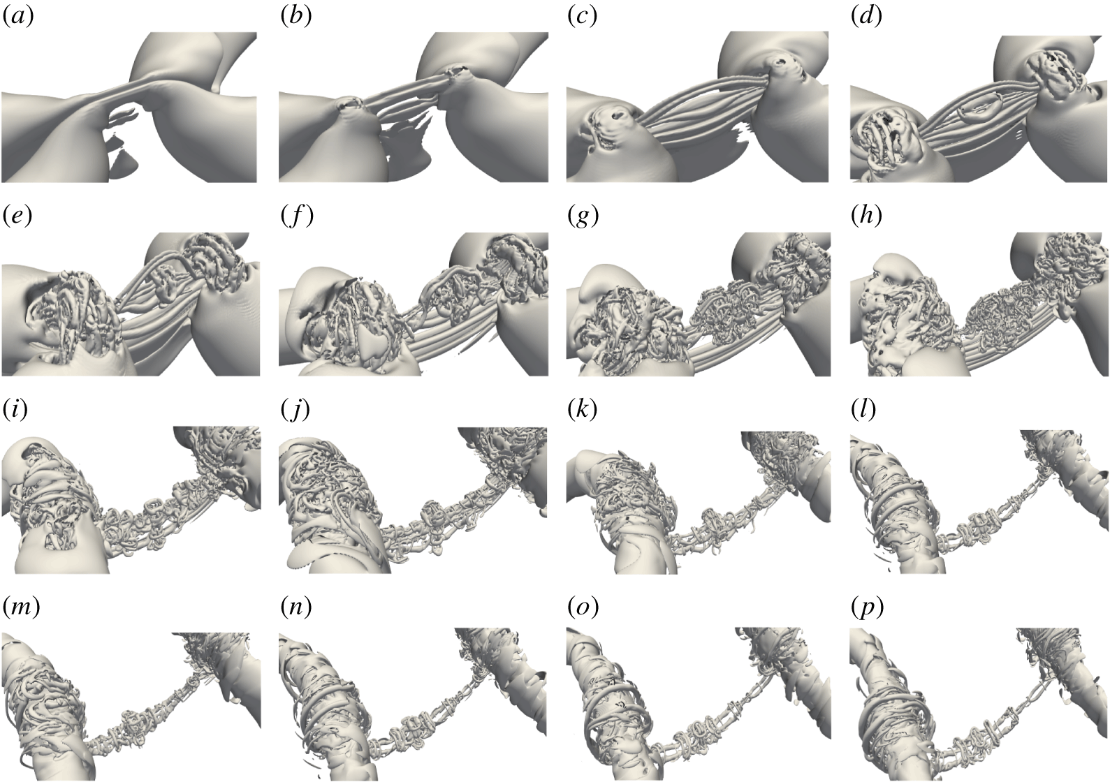
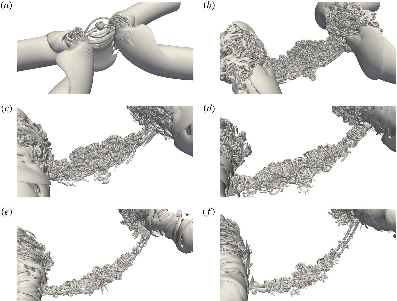
Figure 18 displays the time evolution of the reconnection process based on the isosurface of the  $\unicode[STIX]{x1D706}_{2}$ criterion for
 $Re=20\,000$ with figure 19 showing the corresponding time-resolved, zoomed-in view of the interaction region. As
 $Re$ increases, the overall dynamics becomes even richer and more complicated due to the generation and interaction of smaller vortices. The early stages at
 $Re=20\,000$ are similar to those observed at
 $Re=9000$: the vortex tubes collide and form vortex sheets, which then naturally form head–tail structures (figure 19a) and subsequently secondary dipoles (figure 19b,c) due to symmetric instability of the plan-jet-like flow consisting of the adjacent parts of the two sheets. Note that more dipoles are developed at this
 $Re$ compared to that at
 $Re=9000$, because the sheets are now thinner and longer at this higher
 $Re$. While the circulation is roughly the same as that at
 $Re=9000$, the Reynolds number of each thread dipole here is almost doubled. These vortex filaments then interact with each other, and reconnect again to form a vortex ring (figures 18b and 19d). The vortex ring further interacts with the thread dipoles under it (figure 19e,f) – generating smaller structures, similar to those observed at
 $Re=9000$. Due to lower viscosity (at high
 $Re$), the smaller scales can survive longer, and further undergo successive reconnections, and break down into even smaller filaments – forming a turbulent cloud avalanche comprised of tangles of slender vortices (figure 19g,h). Meanwhile, under the effect of stretching, the small bridgelets are continuously engulfed into the main bridges, and, as a result, the main bridges become more chaotic than at low
 $Re$. This process continues until the scales where viscous dissipation effects dominate. The turbulent cloud slowly decays when the bridges move apart and the associated strain between them becomes weaker (figure 19j–m). At the later stages (figure 19n–p), only one strong thread dipole is visible, with numerous smaller filaments and vortex rings wrapping around.
Zoomed-in view of  $\unicode[STIX]{x1D706}_{2}^{\ast }$ vortical structures for
 $Re=20\,000$: (a)
 $t^{\ast }=1.60$; (b)
 $t^{\ast }=1.62$; (c)
 $t^{\ast }=1.66$; (d)
 $t^{\ast }=1.69$; (e)
 $t^{\ast }=1.72$; (f)
 $t^{\ast }=1.78$; (g)
 $t^{\ast }=1.85$; (h)
 $t^{\ast }=1.93$; (i)
 $t^{\ast }=2.19$; (j)
 $t^{\ast }=2.36$; (k)
 $t^{\ast }=2.57$; (l)
 $t^{\ast }=2.80$; (m)
 $t^{\ast }=3.00$; (n)
 $t^{\ast }=3.23$; (o)
 $t^{\ast }=3.45$; (p)
 $t^{\ast }=3.70$.

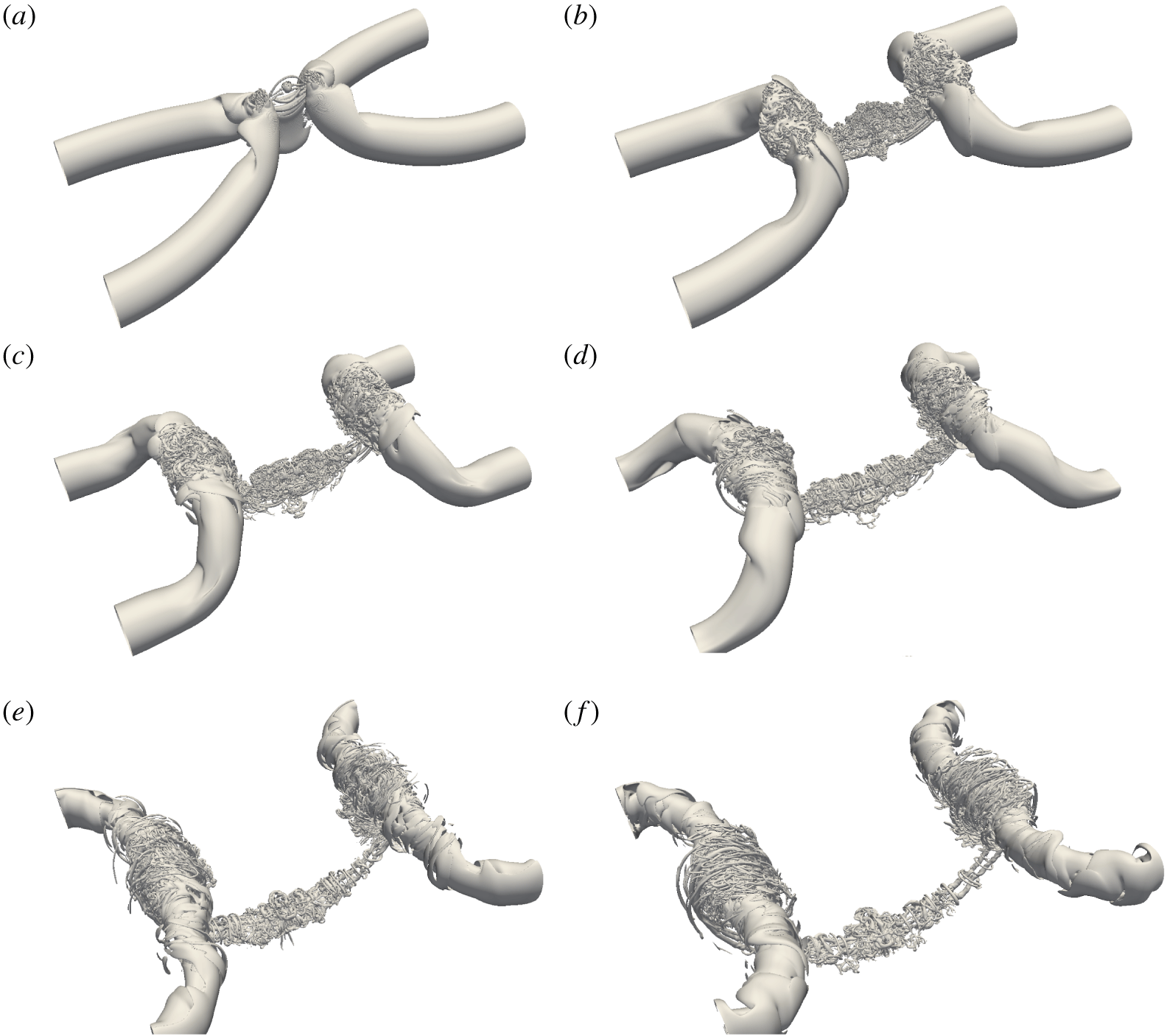
The  $\unicode[STIX]{x1D706}_{2}$ vortical structure at
 $Re=40\,000$: (a)
 $t^{\ast }=1.65$; (b)
 $t^{\ast }=1.96$; (c)
 $t^{\ast }=2.27$; (d)
 $t^{\ast }=2.58$; (e)
 $t^{\ast }=3.34$; (f)
 $t^{\ast }=3.74$. See also supplementary movie 4. Note that the threshold of
 $\unicode[STIX]{x1D706}_{2}^{\ast }$ is chosen as
 $-0.1$.

Figures 20 and 21 show the time evolution of the reconnection process for  $Re=40\,000$. Compared with those at
 $Re=9000$ and
 $20\,000$, the interaction becomes even more rapid. The colliding of the vortex tubes leads to an instantaneous generation of thread dipoles. These dipoles then undergo an enormous number of reconnections, which form an avalanche of large-tangle vortices in a turbulent cloud; see particularly figure 21(b). The continuing stretching between the bridges pulls the cloud into the bridges. The successive reconnections continuously cascade energy to smaller and smaller scales. In particular, the core sizes of the vortex filaments and ring in figure 21(d) are roughly a twentieth of the original core size
 $r_{c}$. A consequence of the strong stretching of the thread causes the structures there to wrap around the stretched threads (see figure 21d). From figures 21(d) to 21(e) to 21(f), the stretching of the threads weakens over these long periods, and hence some finer structures decay, also perhaps undergoing cross-diffusion. Note that the turbulence wrapping around the bridges continues to be dominant because of strong azimuthal stretching by the bridges. The evolutionary dynamics of these tangle of vortices involves many structures and their interactions, which may be examined in detail to characterize and quantify the interactions. Note that our results are for the symmetric thread evolution; the dynamics of similar large-tangle vortices when including the anti-symmetric effect will perhaps not be statistically distinctly different.
A long-standing question in classical turbulence is whether the energy cascade is purely statistical as initially perceived and examined by Kolmogorov, or is based on flow structures, such as a tangle of vortices – which again can be based on the statistics of the structures or derived from the interaction dynamics of deterministic, tractable physical structures. Although the scenario shown here is not exactly the same as proposed by MH, where the initial pair of threads undergoes successive reconnections to smaller and smaller scales, it clearly demonstrates that the vortex reconnection cascade is indeed an essential physical mechanism for turbulence production as well as cascade – presumably involving both deterministic reconnection sequences and avalanche of fine-scale turbulence consisting of tangles of numerous vortices. Hence, the high- $Re$ reconnection results presented here might be helpful in developing a turbulent cascade theory based on the interaction of deterministic vortical structures. Note that the turbulence cascade mechanism proposed by Brenner et al. (Reference Brenner, Hormoz and Pumir2016) involves a scenario intrinsically different from that of MH in that the former suggests that colliding threads form sheets and vortex dipoles and each dipole forming smaller sheet pairs and so on – this scenario does not involve successive reconnections. At the late stage of the reconnection (figure 21f), our results also clearly support the cascade scenario proposed by Melander & Hussain (Reference Melander and Hussain1993) (see also Pradeep & Hussain (Reference Pradeep and Hussain2010), Hussain & Stout (Reference Hussain and Stout2013)) for vortex–turbulence interaction and observed by Goto (Reference Goto2008) in isotropic homogeneous turbulence: each vortex is wrapped around by thinner vortices, which are in turn wrapped around by even thinner vortices, and so on. A similar wrapping scenario has also been observed by Balakrishnan, Thomas & Coleman (Reference Balakrishnan, Thomas and Coleman2011) for vortex ring interacting with the free surface and by Orlandi et al. (Reference Orlandi, Pirozzoli and Carnevale2012) for the interaction of Lamb vortex dipoles. It is worth mentioning that, different from reconnection, this wrapping process does not generate new structures and obviously cannot cause cascade through avalanche.
Zoomed-in view of  $\unicode[STIX]{x1D706}_{2}$ vortical structure for
 $Re=40\,000$: (a)
 $t^{\ast }=1.65$; (b)
 $t^{\ast }=1.96$; (c)
 $t^{\ast }=2.27$; (d)
 $t^{\ast }=2.58$; (e)
 $t^{\ast }=3.34$; (f)
 $t^{\ast }=3.74$.

4.2 Reynolds number effect on circulation transfer and separation distance
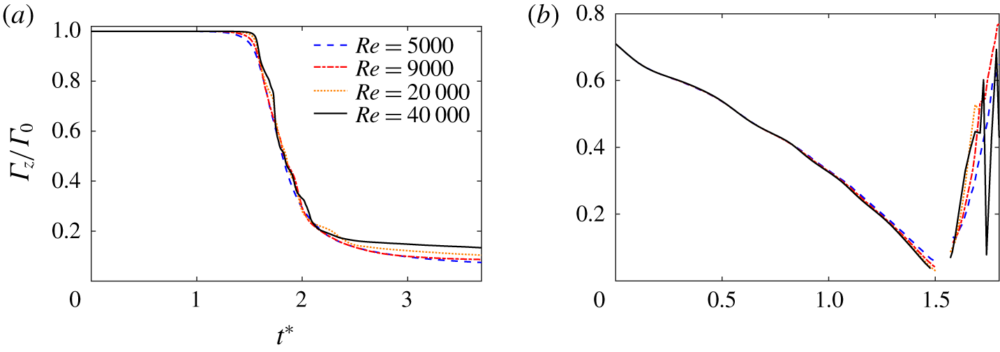
Figure 22 shows the time evolution of  $\unicode[STIX]{x1D6E4}_{z}$ in symmetric plane
 $S_{s}$ for different
 $Re$ values. With increasing
 $Re$, the onset of bridge formation is delayed due to decreasing viscous effect. However, as bridging commences, the accumulation of successive reconnected vortex lines in the bridge is rapid, and the reconnection process is accelerated as
 $Re$ increases. The amplitude of oscillation in circulation transfer increases as
 $Re$ increases, which is consistent with the numerous and rapid successive reconnections found here at higher
 $Re$. It can be seen that
 $\unicode[STIX]{x1D6E4}_{z}$ slowly approaches a constant for all
 $Re$ at the late stage of the reconnection (i.e.
 $t^{\ast }>3.0$). Different from the results at low
 $Re$, where the total circulation transfer
 $\unicode[STIX]{x0394}\unicode[STIX]{x1D6E4}$ was found to monotonically increase with
 $Re$ (HD), the trend seems to be reversed at high
 $Re$ values, i.e.
 $\unicode[STIX]{x0394}\unicode[STIX]{x1D6E4}$ decreases as
 $Re$ increases. This reduced circulation transfer is due to the reduced reconnection in the symmetric plane, which can be explained as follows. The motion induced by the bridges can cause a thread pair to collide near the bridges, hence causing off-plane reconnections and producing a vortex ring in its centre (e.g. figure 4(d) for
 $Re=9000$, figure 19(d) for
 $Re=20\,000$ and figure 21(a) for
 $Re=40\,000$). In reality, this ring is of an elliptical shape, and evolves by switching axis; as a result, in the symmetric plane the two sides of the ring move apart from the collision plane. This is why this ring does not go through another reconnection (see D1 in figure 8h), hence decreasing the circulation transfer in the symmetric plane. Our results also indicate that the total circulation transfer would become zero as
 $Re$ approaches
 $\infty$, which is consistent with the claim that, in the inviscid case, reconnection would not happen.
Time evolution of (a)  $\unicode[STIX]{x1D6E4}_{z}$ and (b) separation distance
 $\unicode[STIX]{x1D6FF}(t)$ at different
 $Re$ values.

Figure 22(b) shows the time evolution of separation distance  $\unicode[STIX]{x1D6FF}(t)$ for different
 $Re$ values. It is interesting to note that
 $\unicode[STIX]{x1D6FF}(t)$ before reconnection almost collapses for high
 $Re$ values, which is consistent with the finding by Kimura & Moffatt (Reference Kimura and Moffatt2014). This is because the phase of vortex approach is mainly inviscid, and its time scale is independent of viscosity provided
 $Re$ is sufficiently large. When reconnected, the bridge retracts rapidly away from the reconnected region. Since the curvature increases with
 $Re$, the retracting motion of the bridges increases as
 $Re$ increases. Oscillation of the separation distance after reconnection is observed for the highest
 $Re$ (i.e.
 $40\,000$). This is because a tangle of successive reconnections forms a turbulent cloud, whose centroid ceases to be meaningful as the vortex centre.
4.3 Enstrophy and peak vorticity scaling, and energy spectra
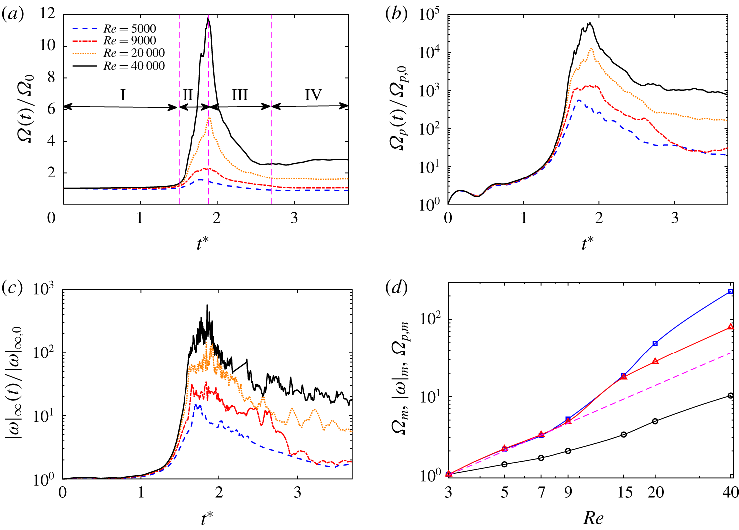
Time evolution of (a) volume-averaged enstrophy  $\unicode[STIX]{x1D6FA}(t)$, (b) volume-averaged enstrophy production
 $\unicode[STIX]{x1D6FA}_{p}(t)$ and (c) peak vorticity magnitude
 $|\unicode[STIX]{x1D74E}|_{\infty }$ at different
 $Re$; and (d)
 $Re$ dependence of the global peak
 $\unicode[STIX]{x1D6FA}(t)$ (circle),
 $\unicode[STIX]{x1D6FA}_{p}(t)$ (square) and
 $|\unicode[STIX]{x1D74E}|_{\infty }$ (triangle). The dashed line in (d) denotes the power-law scaling
 $Re^{1.75}$ suggested by HD.

The enstrophy density  $\unicode[STIX]{x1D74E}^{2}/2$ evolution equation is
 $$\begin{eqnarray}\displaystyle \frac{\text{D}\unicode[STIX]{x1D74E}^{2}/2}{\text{D}t}=\unicode[STIX]{x1D74E}\unicode[STIX]{x1D64E}\unicode[STIX]{x1D74E}+\unicode[STIX]{x1D708}\unicode[STIX]{x1D6FB}^{2}(\unicode[STIX]{x1D74E}^{2}/2)-\unicode[STIX]{x1D708}(\unicode[STIX]{x1D735}\unicode[STIX]{x1D74E})^{2}, & & \displaystyle\end{eqnarray}$$
where  $\text{D}/\text{D}t$ denotes the substantial derivative, and the terms on the right-hand side represent enstrophy production
 $\unicode[STIX]{x1D6FA}_{p}$, diffusion
 $\unicode[STIX]{x1D6FA}_{d}$ and dissipation
 $\unicode[STIX]{x1D6FA}_{\unicode[STIX]{x1D716}}$, respectively, and
 $\unicode[STIX]{x1D64E}=(\unicode[STIX]{x1D735}\boldsymbol{u}+\unicode[STIX]{x1D735}\boldsymbol{u}^{T})/2$ is the rate-of-strain tensor.
Figure 23(a) shows the evolution of the enstrophy  $\unicode[STIX]{x1D6FA}(t)$ for different
 $Re$ values. Based on the enstrophy evolution, the reconnection process can be decomposed into four different regimes. From
 $t^{\ast }=0$ to
 $1.5$ (regime I), the flow evolution is essentially inviscid, and the two vortex tubes approach each other under curvature-induced self-induction. During this first period,
 $\unicode[STIX]{x1D6FA}(t)$ remains approximately constant as the vortices experience no significant deformation. In regime II, as the tubes become significantly closer to each other, they start to reconnect and generate numerous small scales. Consequently,
 $\unicode[STIX]{x1D6FA}(t)$ experiences rapid growth, which also corresponds to a rapid increase in energy dissipation. It is not surprising that the peak of
 $\unicode[STIX]{x1D6FA}(t)$ increases as
 $Re$ increases. However, the time at which the peak is reached seems to be less dependent on
 $Re$. After the peak, the interaction slows down, and the enstrophy experiences a rapid drop (regime III). When the reconnection process stops, the enstrophy remains constant again (regime IV).
Consistent with the enstrophy  $\unicode[STIX]{x1D6FA}(t)$, its production
 $\unicode[STIX]{x1D6FA}_{p}(t)$ (figure 23b) also experiences rapid growth as the reconnection starts. Although enstrophy
 $\unicode[STIX]{x1D6FA}(t)$ remains approximately constant in regime IV, the enstrophy production is still relatively large for the high-
 $Re$ case, which is balanced out by the enstrophy dissipation
 $\unicode[STIX]{x1D6FA}_{\unicode[STIX]{x1D716}}$. Figure 23(d) shows the
 $Re$ scaling of the peak
 $\unicode[STIX]{x1D6FA}(t)$ and
 $\unicode[STIX]{x1D6FA}_{p}(t)$. Based on the low-
 $Re$ data, HD observed that the enstrophy production scales with
 $Re$ following a power law
 $Re^{1.75}$. Our results suggest that both of the peaks of the enstrophy and its production seem to grow faster than the power law suggested by HD. This faster growth rate is consistent with our findings based on flow visualization that finer and finer scales are generated as
 $Re$ increases.
The growth of  $|\unicode[STIX]{x1D74E}|_{\infty }(t)$ is directly related to the presence of the FTS of the solution of the Euler or Navier–Stokes equations: the formation of an FTS must be accompanied by a blow-up of the vorticity field (Beale, Kato & Majda Reference Beale, Kato and Majda1984). From the FTS perspective, given a smooth initial condition of finite energy, there is still no convincing evidence of its existence (Doering Reference Doering2009; Moffatt & Kimura Reference Moffatt and Kimura2019b). Interaction of anti-parallel vortex tubes has been previously employed to give insights into this problem (Kerr Reference Kerr1993; Hou & Li Reference Hou and Li2006). Figure 23(c) shows the evolution of vorticity maximum
 $|\unicode[STIX]{x1D74E}|_{\infty }(t)$ for different
 $Re$. Similar to enstrophy
 $\unicode[STIX]{x1D6FA}(t)$,
 $|\unicode[STIX]{x1D74E}|_{\infty }(t)$ also grows rapidly during the reconnection and reaches the peak almost at the same time as
 $\unicode[STIX]{x1D6FA}(t)$. However, unlike
 $\unicode[STIX]{x1D6FA}(t)$, which is a volume-averaged quantity,
 $|\unicode[STIX]{x1D74E}|_{\infty }(t)$ exhibits strong oscillations, especially for the high-
 $Re$ cases. The
 $Re$ scaling of the peak of vorticity maximum
 $|\unicode[STIX]{x1D74E}|_{\infty }(t)$ is also included in figure 23(d). It is interesting that
 $Re$ dependence of peak vorticity closely follows the enstrophy production curve at low
 $Re$ and departs at higher
 $Re$, for which distinct turbulent clouds are observed. As the vortex tubes approach each other, the cores are flattened to sheets that become unstable and break up through Kelvin–Helmholtz instability – forming a row of smaller vortex tubes with lower
 $Re$. This core-flattening phenomenon might be a possible reason for reduced vorticity peak growth at higher
 $Re$, suggesting that an FTS might not be developed for such configuration. Recently, Moffatt & Kimura (Reference Moffatt and Kimura2019b) in their study of FTS argued that the vortex-core flattening would not occur if the separation distance between the vortices is small compared with their radius of curvature at the closest points and if
 $Re$ is exceptionally large, and suggested that an FTS might still be possible for inviscid flow. However, Moffatt & Kimura (Reference Moffatt and Kimura2019a) also showed that even if there is no core-flattening effect, vortex reconnecton involves no strict finite-time mathematical singularity. It is also worth mentioning that the decreased growth of vorticity peak at high
 $Re$ observed here might also be due to the inadequacy of the numerical resolution to resolve the extreme vorticity events. This needs to be verified with higher-resolution simulations, which remains as a computational challenge at the current stage.
Energy spectrum for different  $Re$ values at the time of peak enstrophy. The straight dashed line corresponds to the
 $-5/3$ slope.

Energy spectra are evaluated at the time of peak enstrophy for different  $Re$ (figure 24). An increase in
 $Re$ generates additional smaller scales while the low-wavenumber content remains mostly the same. The higher-
 $Re$ (i.e.
 ${\geqslant}9000$) cases display a distinct
 $-5/3$ slope for a range of wavenumbers. In addition, the range of
 $-5/3$ slope also enlarges as
 $Re$ increases. In particular, one decade of inertial range (i.e.
 $10\leqslant k\leqslant 100$) can be found for the
 $Re=40\,000$ case. It clearly demonstrates that reconnection of vortex tubes can result in a Kolmogorov spectrum, which supports the long-time claim that classical turbulence can be modelled by the dynamics of a set of vortex tubes or sheets (Frisch Reference Frisch1995). Surprisingly, the low-wavenumber range of the spectrum seems to also have a slope of
 $k^{-5/3}$ for
 $k<7$ and a very steep one (approximately
 $k^{-5}$) in the range
 $7<k<10$. However, by comparing that with the Gaussian vorticity profile case (see appendix B), we find that the spectrum at these low wavenumbers is mainly determined by the initial geometry. It would be interesting to perform similar scale-locality and structural analysis as performed at
 $Re=9000$ for the higher-
 $Re$ cases; however, this is not currently possible due to the limited computational resources and insufficient saved data.
5 Concluding remarks
In summary, we have found clear evidence of the vortex reconnection cascade scenario, particularly at  $Re=9000$: the threads, under first reconnection, form head–tail structures, and develop into a series of thread dipoles; some of the dipoles under the second generation of reconnection form vortex rings and hairpin packets. During reconnection, a
 $-5/3$ spectrum is observed in the large-wavenumber ranges, which has been shown to be due to successive reconnections and associated vortex stretching. As
 $Re$ increases, the energy is more rapidly transferred to finer and finer scales through successive reconnections – forming a turbulent cloud avalanche consisting of a tangle of slender vortex filaments and rings. The
 $-5/3$ regime becomes more pronounced with increasing
 $Re$. In addition, we also observed an inverse cascade at smaller wavenumbers via the pairing of the bridges. The present work highlights the importance of reconnection for the physical mechanism of energy cascade in classical turbulence. A further theoretical investigation is required for a clear understanding of the relationship between the reconnection dynamics and statistics of turbulence energy cascade. In real flows, the threads, which are very sensitive to a Kelvin–Helmholtz instability due to their stretching by the bridges, are likely to break up asymmetrically at higher Reynolds numbers. It is, therefore, an important future study to quantify the effect of anti-symmetric perturbations on reconnection.
Acknowledgements
Computational and visualization resources provided by Texas Tech University HPCC, TACC Lonestar and XSEDE are acknowledged. We thank Neil Vaz and Christopher Bryson for helpful discussions.
Supplementary movies
Supplementary movies are available at https://doi.org/10.1017/jfm.2019.905.
Appendix A. Detailed comparison between the different initial conditions
(a) Illustration of calculation of  $\unicode[STIX]{x1D6E4}_{z}$,
 $\unicode[STIX]{x1D6E4}_{t}$. (b) Circulation along the tube
 $\unicode[STIX]{x1D6E4}_{t}$ as a function of
 $z$ for the initial condition of MH.

For anti-parallel vortex reconnection, many studies employ the initial configuration suggested by MH. It is easy to overlook the fact that the sinusoidal perturbation introduces an inherent error along the circulation along the axis. Here we briefly explain the source. The vorticity field of the MH initial configuration is specified as
 $$\begin{eqnarray}\displaystyle \unicode[STIX]{x1D74E}(\boldsymbol{x})=\unicode[STIX]{x1D714}(r^{\prime })[p\cos \unicode[STIX]{x1D6FC}f^{\prime }(z)\boldsymbol{e}_{\boldsymbol{x}}+p\sin \unicode[STIX]{x1D6FC}f^{\prime }(z)\boldsymbol{e}_{\boldsymbol{y}}+\boldsymbol{e}_{\boldsymbol{z}}], & & \displaystyle\end{eqnarray}$$
where  $\unicode[STIX]{x1D714}(r^{\prime })$ is the compact Gaussian distribution, same as equation (2.4).
For a given point  $\boldsymbol{x}_{1}=(x_{1},y_{1},z_{1})$, the radius
 $r^{\prime }$ (figure 25a), based on MH, is determined as
 $$\begin{eqnarray}\displaystyle r^{\prime }=\sqrt{[x_{1}-x_{0}-p\cos \unicode[STIX]{x1D6FC}\cos (z_{1})]^{2}+[y_{1}-y_{0}-p\cos \unicode[STIX]{x1D6FC}\cos (z_{1})]^{2}}. & & \displaystyle\end{eqnarray}$$
Then the vorticity at point  $\boldsymbol{x}_{1}$ is given as
 $$\begin{eqnarray}\displaystyle \unicode[STIX]{x1D74E}(\boldsymbol{x}_{1})=\unicode[STIX]{x1D714}(r^{\prime })[-p\sin \unicode[STIX]{x1D6FC}\sin (z_{1})\boldsymbol{e}_{\boldsymbol{x}}+p\cos \unicode[STIX]{x1D6FC}\sin (z_{1})\boldsymbol{e}_{\boldsymbol{y}}+\boldsymbol{e}_{\boldsymbol{z}}]. & & \displaystyle\end{eqnarray}$$
For this configuration, the circulation is constant along the  $z$ direction, i.e.
 $\unicode[STIX]{x1D6E4}_{z}=\int _{S_{z}}\unicode[STIX]{x1D714}_{z}\,\text{d}S_{z}=\unicode[STIX]{x1D6E4}_{0}$, where
 $S_{z}$ is the plane perpendicular to the
 $z$ axis.
The vorticity along the vortex tube is given as
 $$\begin{eqnarray}\displaystyle \unicode[STIX]{x1D714}_{\boldsymbol{t}}=\unicode[STIX]{x1D74E}(\boldsymbol{x}_{1})\boldsymbol{\cdot }\boldsymbol{t}/|\boldsymbol{t}|, & & \displaystyle\end{eqnarray}$$
where  $\boldsymbol{t}$, given in equation (2.7), is the tangent vector to the vortex centroid curve that is associated with
 $\boldsymbol{x}_{1}$.
The circulation along the tube can be calculated as  $\unicode[STIX]{x1D6E4}_{\boldsymbol{t}}=\int _{S_{\boldsymbol{t}}}\unicode[STIX]{x1D714}_{\boldsymbol{t}}\,\text{d}S_{\boldsymbol{t}}$, where
 $S_{\boldsymbol{t}}$ is the perpendicular surface tangent to the vortex axis shown in figure 25(a). Figure 25(b) shows
 $\unicode[STIX]{x1D6E4}_{\boldsymbol{t}}$ as a function of
 $z$. It is evident that
 $\unicode[STIX]{x1D6E4}_{\boldsymbol{t}}$ is exactly equal to
 $\unicode[STIX]{x1D6E4}_{0}$ only at planes
 $z=-\unicode[STIX]{x03C0},0$ and
 $\unicode[STIX]{x03C0}$, and has approximately
 $2\,\%$ variation around
 $z=\pm \unicode[STIX]{x03C0}/2$.
Time evolution of (a) circulation transfer, (b) energy, (c) enstrophy and (d) maximum vorticity for current (solid line) and MH initial configuration ( $\circ$) at
 $Re=5000$.

Here we present detailed comparisons for these two different configurations based on the simulation results at  $Re=5000$. Figure 26(a) is the circulation transfer in the symmetric and collision planes. Figure 26(b–d) shows the time evolution of the volume-integrated energy, enstrophy and the maximum vorticity. The differences between the two cases for all quantities are relatively small, suggesting that the results obtained based on the previous initial condition by MH and others still hold.
Appendix B. Vortex reconnection with a Gaussian initial profile
To prevent the peripheral region of the vortex from initiating the reconnection so that the reconnection is more focused, we employ an initial condition with a compact support vorticity profile. To demonstrate that the results presented are not restricted to our particular initial condition, we perform here an additional simulation with a different vorticity profile, namely Gaussian:
 $$\begin{eqnarray}\displaystyle \unicode[STIX]{x1D714}(r)=\frac{\unicode[STIX]{x1D714}}{\unicode[STIX]{x03C0}r_{c}^{2}}e^{-r^{2}/r_{c}^{2}}. & & \displaystyle\end{eqnarray}$$
(a) Time evolution of circulation transfer and (b) energy spectrum at  $Re=9000$ for the Gaussian profile case.

Figure 27(a) shows the time evolution of  $\unicode[STIX]{x1D6E4}_{z}$ and
 $\unicode[STIX]{x1D6E4}_{x}$ for the Gaussian case. Different from the compact support case, vortex reconnection immediately starts when the simulation starts. As a result,
 $\unicode[STIX]{x1D6E4}_{z}$ continuously decreases. Evolutions of both
 $\unicode[STIX]{x1D6E4}_{z}$ and
 $\unicode[STIX]{x1D6E4}_{x}$ are similar to those for the compact support case. The only apparent difference is that the rate of reconnection is slightly slower for the Gaussian case. Figure 28 shows the evolution of
 $\unicode[STIX]{x1D706}_{2}$ vortical structures for the Gaussian case. The overall dynamics is quite similar to that of the compact support case – suggesting that our results with compact vorticity support are generic. We further show the energy spectrum at various instants in 27(b). At
 $t^{\ast }=0$, most energy is concentrated at small scales with a Gaussian profile. The energy at large wavenumbers emerges as the vortex tubes approach each other. At
 $t^{\ast }=3$ (the time of the maximum enstrophy), the spectrum also develops a distinct power law with
 $-5/3$ slope. In addition,
 $-5/3$ spectrum does not occur in the low-wavenumber range for this case.
Vortical structures visualized with  $\unicode[STIX]{x1D706}_{2}^{\ast }=-0.1$ for the Gaussian profile case: (a)
 $t^{\ast }=0$; (b)
 $t^{\ast }=2.2$; (c)
 $t^{\ast }=2.7$; (d)
 $t^{\ast }=3.0$, (e)
 $t^{\ast }=3.6$; (f)
 $t^{\ast }=4.7$.

Appendix C. Comparison between simulations using single- and double-precision arithmetic at $Re=9000$

To demonstrate the effect of computational precision arithmetic, we perform simulation with single and double precision at  $Re=9000$ with the full domain
 $[-\unicode[STIX]{x03C0}~\unicode[STIX]{x03C0}]^{3}$. The grid resolution is the same at
 $1024^{3}$ for both cases. Figure 29(a) compares the time evolution of circulation transfer between the two cases. For the double-precision case, the result using the full domain size agrees excellently with that of imposing symmetry condition (figure 10a). Good congruence can be observed between single- and double-precision cases for both
 $\unicode[STIX]{x1D6E4}_{x}$ and
 $\unicode[STIX]{x1D6E4}_{z}$ until
 $t^{\ast }=1.8$, when approximately
 $50\,\%$ of the circulation is transferred. Then, the circulation transfer between these two cases deviates, with the circulation transfer for the single-precision case being slightly larger.
Time evolution of (a) circulation transfer and (b) asymmetric energy for single and double precision at  $Re=9000$.

Vortical structures visualized with  $\unicode[STIX]{x1D706}_{2}^{\ast }=-0.1$ for the single-precision case: (a)
 $t^{\ast }=1.72$; (b)
 $t^{\ast }=1.86$; (c)
 $t^{\ast }=2.34$; (d)
 $t^{\ast }=2.79$.

To quantify the strength of the asymmetric perturbation, the asymmetric energy is defined as
 $$\begin{eqnarray}\displaystyle E_{u}(t)=\frac{1}{V}\int \boldsymbol{u}_{u}(x,y,z,t)\boldsymbol{\cdot }\boldsymbol{u}_{u}(x,y,z,t)\,\text{d}V, & & \displaystyle\end{eqnarray}$$
where  $\boldsymbol{u}_{u}$ represent the asymmetric velocity components, which do not satisfy the symmetric conditions defined in equations (2.9) and (2.10). Energies
 $E_{u}(t)$ for both the single- and double-precision cases are shown in figure 29(b). Initially, the asymmetric energy
 $E_{u}(t)$ is around
 $10^{-16}$ and
 $10^{-32}$ for the single- and double-precision cases, respectively. For both cases,
 $E_{u}(t)$ experiences slow increases during the advection phase, but increases rapidly as reconnection starts. At the late stage of the reconnection,
 $E_{u}(t)$ for the single-precision case becomes non-negligible, while
 $E_{u}(t)$ for the double-precision case is still relatively small – less than the initial value of the single-precision case. This demonstrates that double-precision arithmetic can effectively suppress the symmetry-breaking phenomenon. However, since the rate of increase of asymmetric energy increases with
 $Re$, it suggests that the double-precision arithmetic might also become insufficient at higher
 $Re$.
Figure 30 further shows the vortical structures for the single-precision case. The structure at  $t^{\ast }=1.72$ is almost identical to that shown in figure 4(a) for the double-precision case, where several thread dipoles are formed. However, the structures at late times are quite different from those of the double-precision case, where numerous asymmetric structures are observed. Compared with those in figure 6, the vortex rings and organized hairpin packets are less apparent in this case.