Introduction
Both the contrast sensitivity function (CSF) and visual acuity have become common measures for quantifying vertebrate spatial vision. The CSF is usually determined using luminance-modulated spatial sine-wave gratings, where visual sensitivity at a given grating frequency is defined as the inverse of Michelson contrast at the threshold of grating detection. In humans, it has been shown that the CSF can be related directly to the manner in which the visual system processes spatial information from photon capture through to signal detection (De Valois & De Valois, Reference De Valois and De Valois1990; Regan, Reference Regan and Cronly-Dillon1991).
Modeling the CSF has been an area of active research for many years. Models developed range from relatively simple mathematical descriptions such as a twin Gaussian function (Uhlrich et al., Reference Uhlrich, Essock and Lehmkuhle1981), through to more complex black box models. Yang et al. (Reference Yang, Qi and Makous1995), for example, have derived a three-stage signal processing model combining two linear spatial filters with a final nonlinear detection process. Recently, Watson and Ahumada (Reference Watson and Ahumada2005) have derived a five-stage model, which again incorporates a cascade of spatial filters and also addresses the multichannel nature of spatial information transfer through the visual system (Watson & Solomon, Reference Watson and Solomon1997). An interesting feature of the Watson and Ahumada model is the addition of a filtering process, which accounts for the well-known oblique effect as described by Campbell et al. (Reference Campbell, Kulikowski and Levinson1966).
Although these models have been successful in describing the human photopic CSF, they are all examples of a particular genre of model, which is limited in its ability to link the nature of the CSF through to detailed elements of underlying visual neurophysiology. An alternative theoretical signal modulation transfer (MTF) modeling approach adopted by both Barten (Reference Barten1999) and Rovamo et al. (Reference Rovamo, Mustonen and Nasanen1994) does specifically address this linkage. The Barten variant, in particular, is detailed in its incorporation of the key physiological loci in the visual system, which impact CSF. Specifically, stages quantifying optical attenuation, quantum (transduction) efficiency, receptor sampling, lateral inhibition, area signal summation effects, neural noise, and a final cortical detection factor are incorporated. In each stage, equation parameters define the magnitude of a specific physiological response. Of particular importance is the fact that previous studies of this model have compared calculated parameter values with those obtained by direct physical measurement. For example, Jarvis and Wathes (Reference Jarvis and Wathes2007) found that values of the optical modulation transfer function (OMTF) calculated from application of the Barten theory to CSF data, correlated closely with appropriate values obtained through double-pass retinal examination studies. This was substantiated for a range of vertebrate species. Calculations of ganglion cell receptive field sizes (relevant to the role of lateral inhibition) were also found to correlate well with values obtained from electrophysiology. Again, this support for the model was obtained from a range of vertebrates including the human (Jarvis & Wathes, Reference Jarvis and Wathes2008).
When applied to measured photopic CSF data, the Barten model can accurately describe human CSF data measured for a wide range of stimulus conditions including luminance level, stimulus size, and eccentricity (Barten, Reference Barten1999). Similar success has been found when the model is applied to photopic CSF measured in a large range of nonhuman species (Jarvis & Wathes, Reference Jarvis and Wathes2007, Reference Jarvis and Wathes2008; Gover et al., Reference Gover, Jarvis, Abeyesinghe and Wathes2009; Jarvis et al., Reference Jarvis, Abeyesinghe, McMahon and Wathes2009). In general, the shape of the CSF shows that both human and nonhuman spatial vision demonstrate a band-pass characteristic. Typically, as spatial frequency increases, photopic contrast sensitivity increases, passes through a maximum, and then decreases toward unity at a limiting frequency often referred to as acuity. The effect of changing stimulus luminance on CSF is also well documented in the literature. After an initial invariance, both acuity and overall magnitude of the CSF reduce as stimulus luminance is lowered from high photopic levels down to levels associated with scotopic vision. This behavior is observed in all species where the effect of luminance on CSF has been studied (see, e.g., Barten, Reference Barten1999; Jarvis & Wathes, Reference Jarvis and Wathes2008; Douglas, Reference Douglas, Breed and Moore2010 for reviews of relevant studies in human and nonhuman vision). At low luminance, the CSF tends to display low-pass rather than band-pass filtering behavior.
In the modeling of human CSF, Barten (Reference Barten1999) found that the theoretical signal transfer approach became limited at low luminance; the theory tended to underestimate low frequency sensitivity and overestimate high frequency response. Yang et al. (Reference Yang, Qi and Makous1995) found an identical discrepancy in their modeling of the low luminance CSF data obtained by van Nes and Bouman (Reference van Nes and Bouman1967). Similar and significant deviations between measurement and theory were also found from studies of low luminance CSF in the macaque, goldfish, and cat (Jarvis & Wathes, Reference Jarvis and Wathes2008).
In this communication, we address the observed limitations of the theoretical model developed by Barten when applied to vertebrate CSF at low luminance. Specifically, we define changes, which should be made to the model framework in the specification of CSF and acuity with scotopic vision. This particular signal transfer model is chosen because of its ability to relate CSF to underlying physiological processes and it is these that are addressed in the reengineering process. The refined theory is tested with scotopic CSF data obtained from the human, macaque, cat, and owl monkey; this last species defining an interesting nocturnal species with a relatively high density of rods in the fovea. Our study also reveals specific optical and retinal factors, which are of particular importance in defining the scotopic CSF in each of the species examined.
Theoretical framework
Signal transfer under photopic conditions
The basic mathematical formulation for the photopic CSF as derived by Barten (Reference Barten1999) and Rovamo et al. (Reference Rovamo, Mustonen and Nasanen1994) is given by:

where S denotes the CSF in terms of spatial frequency u (c/deg). The terms K and A relate to cortical signal detection and spatial integration, respectively. The term O is given by:

where OMTF is the MTF describing the effect of optical attenuation and MTFr the MTF associated with retinal sampling. The function H describes the action of lateral inhibition in the retina and the function N the total noise in the visual system, which is a combination of photon and neural noise. Each of the functions given in eqns. (1) and (2) are analytic and contain parameters, which can be specifically related to both optical and neural mechanisms. In detail, the functional form of O, H, and A in the Barten model variant differs from that given by Rovamo et al. Full details of both model variants, their equations, and our reasons for choosing the Barten framework in our study are given in Appendix 1. Details of the calculation of parameters contained within the model and their relationship to underlying neurophysiology are also given. In summary, the salient features of the model are as follows.
The parameters for O, H, and A are:
u *: which defines OMTF and is the spatial frequency at half its maximum value. This parameter can be algebraically calculated from measured high frequency CSF data, and the resulting OMTF correlates well with that obtained directly through the double-pass optical probe technique (Jarvis & Wathes, Reference Jarvis and Wathes2007).
σ: which defines MTFr and represents the standard deviation of the ganglion cell sampling line spread function. For a given species, estimations of this parameter can be made from retinal ganglion cell density.
u 0: which defines function H and represents the spatial frequency above which lateral inhibition ceases to operate. Determinations of this parameter can be made from photopic low frequency measured CSF.
X max, R max: representing the upper retinal size and frequency limits, respectively, of spatial integration. These two parameters define function A for a given species. This function also contains a variable term, which represents the overall angular size (deg) of the stimulus. Again, both X max and R max can be algebraically derived from measured photopic CSF.
The function N in the model not only contains photon and neural noise but is itself a function of H. This term is given by:

where N qt and N it represent photon and internal neural noise, respectively. Note that the use of noise in this analysis is in terms of contrast noise as defined by Pelli (Reference Pelli and Blakemore1990).
Photon noise is an important consideration in the analysis of CSF and can impair the detection of a visual object, particularly at low luminance. This noise component can be related to both quantum efficiency (η) and retinal illuminance (I) (Pelli, Reference Pelli and Blakemore1990; Barten, Reference Barten1999). The final expression derived for N qt by Barten (Reference Barten1999) is given by

where ρ defines a photon conversion factor and for most light sources is approximately 1.2 × 10⁶ photons/s/deg2/Td (Scheibner & Baumgardt, Reference Scheibner and Baumgardt1967; Barten, Reference Barten1999). In eqn. (4), quantum efficiency η is defined as the ratio of the number of photons causing excitation of the photoreceptors to the total number of photons entering the eye. It therefore correlates closely with what has been described as transduction efficiency (Pelli, Reference Pelli and Blakemore1990). As shown in Appendix 1, the equation parameters η and N it can be combined to form the parameter product ( ). This mathematical procedure effectively reduces the total number of parameters to be evaluated in the model by one.
The last term K in eqn. (1) is a constant, which defines a cortical detection factor incorporating the Crozier coefficient. This coefficient represents a basic signal/noise constant for the detection of a luminance signal (Roufs, Reference Roufs1974).
Eqn. (4) shows that retinal illuminance must be known in order to calculate photon noise. For the human, this photometric quantity can be calculated directly from luminance providing pupil diameter is known. In nonhuman species, knowledge of posterior nodal distance (PND) is also required (Berkley, Reference Berkley1976; Hughes, Reference Hughes and Crescitelli1977).
It was demonstrated in a previous publication (Jarvis & Wathes, Reference Jarvis and Wathes2008) that the post-optical parameter values in the photopic equations are fixed and unique for a given species. If these values are known, it was found that the theoretical model is capable of predicting CSF remarkably accurately for changes in both stimulus (photopic) luminance and overall stimulus size, by simply applying appropriate values for retinal illuminance, stimulus size, and the optical parameter u *. However, when the theory is applied to grating detection at low luminance levels, significant and consistent deviations from directly measured CSF become evident, as described above. In the next section, we re-examine key assumptions made in the derivation of the photopic theory and propose modifications for scotopic lighting conditions.
Signal transfer under scotopic conditions
In the analysis of scotopic CSF, it will be assumed that both the signal transfer basis for the theory and its functional form are correct. Each important stage in the mathematical framework will be, however, re-examined with respect to the physiological meaning and numerical value of individual equation parameters. Initially, we examine neural factors (starting with retinal sampling) under scotopic conditions and then finally address the optical mechanism.
Retinal sampling
Under photopic conditions, the retinal sampling parameter σ is calculated from maximum ganglion cell density for a given species (which coincides with the center of the fovea if this exists). Under scotopic conditions, it would seem reasonable to assume that under free-view conditions, ganglion cell density at a location on the retina where rod density is at its maximum value is more appropriate for defining the sampling parameter. In most vertebrates, this will have an eccentric location. The importance of off-axis viewing in detection tasks at low luminance has already been inferred by Hess (Reference Hess, Hess, Sharpe and Norby1990) and in studies of both cat CSF (Pasternak & Merigan, Reference Pasternak and Merigan1981) and rod topography (Steinberg et al., Reference Steinberg, Reid and Lacy1973). In the following treatment, we therefore make the distinction between equation parameters, which relate to photopic and central vision by denoting the function notation (c). Likewise, parameters relating to scotopic and therefore eccentric vision are given the notation (e).
Internal neural noise ( )
 )
Neural information generated by a given retinal image will be transported through to the visual cortex by a number of optic nerve fibers in parallel. The magnitude of the signal will vary slightly from fiber to fiber, and this is assumed to be the main cause of internal noise in the theoretical treatment. Clearly, as the ganglion cell density decreases, neural noise will increase. The following relationship (derived by Barten from first principles) defines neural noise at a given eccentricity e (deg) as:

where G denotes ganglion cell density. Therefore, if ganglion cell density varies with eccentricity, so too will neural noise.
Quantum efficiency ()
 )
A change from cone to rod vision requires a careful examination of the quantum efficiency parameter. As discussed above (and shown in Appendix 1), the photopic parameters  and
 can be combined to define the new parameter product
 . For vision at an eccentricity e, where rod density is at its maximum, the equivalent parameter product becomes
 . In principle, this scotopic parameter product can be evaluated in the same fashion as its photopic partner from measured high frequency CSF data. In practice, however, this evaluation technique presents potential accuracy problems because at low luminance, the measured high frequency CSF is usually characterized by relatively few data points. It is, however, possible to directly calculate independently both
 and
 from first principles for a given species as shown in Appendix 2. It will be shown later that the separation of these two parameters reveals an important difference in the behavior of quantum efficiency within diurnal- and nocturnal-biased retinas as luminance reduces.
Optical performance (parameter )
 )
As in the case of  , the parameter
 can be directly calculated from high frequency CSF data (Jarvis & Wathes, Reference Jarvis and Wathes2007). Again, problems arise when using the shape of the measured CSF to evaluate
 at low luminance because of the limited amount of data usually available. Alternative methods for estimating
 were therefore adopted, and full details of these are again given in Appendix 2.
Lateral inhibition (parameter )
 )
The impact of lateral inhibition on contrast sensitivity will change with off-axis viewing because the overall receptive field size of ganglion cells tends to increase (see, e.g., Stone, Reference Stone1965; Peichl & Wassle, Reference Peichl and Wassle1979; Dacey, Reference Dacey1993; Rodieck & Watanabe, Reference Rodieck and Watanabe1993). The lateral inhibition model parameter u 0 is inversely related to ganglion cell receptive field surround size (Barten, Reference Barten1999; Jarvis & Wathes, Reference Jarvis and Wathes2008) and the variation of this parameter with eccentricity can be represented by:

where  and
 .
Eqn. (6) is purely empirical and derived from measured human photopic CSF obtained from a number of studies using nonfoveal imaging (Barten, Reference Barten1999).
Spatial summation (parameters and )
 and
 )
Spatial summation increases in the human retina at eccentric locations (Arden & Weale, Reference Arden and Weale1954), indicating that  . From an analysis of nonfoveal human photopic CSF data, Barten obtained an empirical formula for
 given by:

where  .
The upper limit of spatial integration in terms of maximum number of stimulus cycles for eccentric viewing ( ) is more difficult to assess. A previous study of CSF measured by Robson and Graham (Reference Robson and Graham1981) from a range of vertical strip-shaped gratings centered on the fovea revealed a maximum number of cycles for retinal summation as theoretically expected. The same study revealed that if the strip target was horizontal and imaged well above the fovea, no such limitation in the number of cycles was found. This differentiation between radial and tangential sensitivity is difficult to fully reconcile in the Barten theory. However, based on a) the Robson and Graham contrast sensitivity findings for a radial direction from the fovea and b) the edge of the summation area for a grating imaged on the fovea is located at a distance of 0.5 × maximum number of cycles from the center, Barten suggests that
 should be represented by 0.5
 . In our application of the theory to scotopic conditions, we assume this to be the case. This estimation of
 would only strictly apply if the value of eccentricity is greater than half the size of the grating stimulus.
Cortical detection factor K
The final theoretical neural stage is represented by the cortical detection factor K. Since rods and cones share a common pathway to the brain (D’Zmura & Lennie, Reference D’Zmura and Lennie1986), it is likely that final signal detection is mediated by the same mechanism (Makous, Reference Makous, Werner and Chalupa2004). It is therefore assumed that the numerical value of K remains unaffected by changes in light level.
Analysis of scotopic CSF measurements
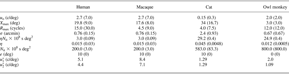
In the following analysis of scotopic CSF, solid curves represent application of the scotopic theory described in the Theoretical framework section to directly measured data for four species. The hatch curves represent the original photopic theory using previously published parameter values (Jarvis & Wathes, Reference Jarvis and Wathes2008). Details of the methodology for estimating numerical values for the scotopic parameters are given in Appendix 2 for each species. A summary of parameter values for both scotopic and photopic conditions is given in Table 1 for each species studied.
Model scotopic parameter values for all four species examined
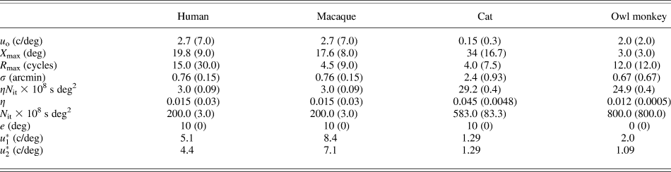
Values given in parenthesis are companion photopic values.
The human response
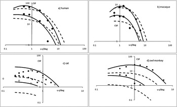
CSF measurements made by van Meeteren and Vos (Reference van Meeteren and Vos1972) with human subjects are shown by the data points in Fig. 1a. This particular study was chosen because the observer used binocular free view, which is compatible with the animal studies outlined below. A relatively large stimulus size was also employed (17 × 11 deg), which enables the scotopic parameter  to be evaluated with more certainty (see above). The upper and lower data sets are for mean grating luminances of 0.01 and 0.001 cd/m2, respectively. This experiment was conducted with natural pupils. The companion values of retinal illuminance (I) are 0.4 and 0.04 Td, respectively (Le Grand, Reference Le Grand1968). Although a specification of the exact luminance for a change in cone to rod vision is difficult, since this will depend upon the testing conditions, it is likely that the two levels of stimulus luminance are scotopic for the human (Schlaer, Reference Schlaer1937). Accordingly, the CSF values shown in Fig. 1a would be for a rod-dominated visual response. Since rod density approaches maximum for an eccentricity of about 10 deg (Osterberg, Reference Osterberg1935; Curcio et al., Reference Curcio, Sloan, Kalina and Hendrickson1990), this value was taken as indicating the appropriate retinal eccentricity (e) dictating scotopic grating detection in free view.
Scotopic spatial contrast sensitivity (CSF). Data points; measured values. Hatch curves; theoretical values calculated from eqn. (1) with photopic parameter values. Solid curves; theoretical values calculated with scotopic parameter values. (a) Human CSF at mean grating luminance levels of 0.01 cd/m2 (upper set of data and curves) and 0.001 cd/m2 (lower set of data and curves). (b) As for (a) but showing macaque CSF result (0.017 and 0.0017 cd/m2). (c) As for (a) but showing cat CSF result (0.0016 and 0.000016 cd/m2). Note that the lowest hatch curve (photopic modeled response at the lower luminance level) is not physically possible since CSF values of less than unity are incurred. (d) As for (a) but showing owl monkey result (0.0011 and 0.00011 cd/m2). Again the photopic model produces untenable CSF values at the lowest luminance level.

In this analysis of measured human CSF, the basic theory is seen to offer a good fit to the CSF data, providing it is re-engineered to rod vision in the manner described in the Theoretical framework section. The original photopic theory shows the undershoot at low frequencies and the overshoot at high frequencies, as originally observed in human vision by Barten (Reference Barten1999).
The macaque response
CSF measurements made by De Valois et al. (Reference De Valois, Morgan and Snodderley1974) at two scotopic levels with the macaque monkey are shown by the data points in Fig. 1b. These data were obtained at stimulus luminances of 0.017 and 0.0017 cd/m2 (upper and lower data sets) and with binocular (free) viewing. Pupil size estimates for the two luminance levels are 6.7 and 6.9 mm (Clarke et al., Reference Clarke, Zhang and Gamlin2003). Using a PND value of 12 mm (Pettigrew et al., Reference Pettigrew, Dreher, Hopkins, McCall and Brown1988), the corresponding levels of retinal illuminance are 1.17 and 0.124 Td. Since the macaque has a rod topography similar to the human (Goodchild et al., Reference Goodchild, Ghosh and Martin1996), 10-deg eccentricity was taken as appropriate for grating detection at low luminances. As for the human, the scotopic theory fits the measured CSF data well, whereas the photopic theory provides a CSF, which displays low frequency undershoot and high frequency overshoot.
The cat response
The solid data points in Fig. 1c are measured CSF values for the cat as determined by Pasternak and Merigan (Reference Pasternak and Merigan1981). Data are given for grating mean luminances of 0.0016 and 1.6 × 10⁻⁵ cd/m2 (upper and lower data sets) and are taken to be scotopic for this species. Using the PND value given by Vakkur et al. (Reference Vakkur, Bishop and Kazak1963) and pupil size data from Hammond and Mouat (Reference Hammond and Mouat1985), the corresponding retinal illuminance levels are 0.5 and 0.005 Td. As for the human and the macaque, an eccentricity value of 10 deg was taken as appropriate for low luminance detection tasks by the cat in free view since maximum rod density is reached at about this value (Steinberg et al., Reference Steinberg, Reid and Lacy1973).
The open data points in Fig. 1c are CSF measurements obtained from a more recent study of cat scotopic CSF (Kang et al., Reference Kang, Reem, Kaczmarowski and Malpeli2009) and are for two luminances close to those given in the Pasternak study. Upper and lower data sets are again for the highest and lowest luminance levels, respectively (note that the data point at 0.1 c/deg is within the lower set).
A close inspection of Fig. 1c reveals that at each luminance level, the photopic theory underestimates CSF by a substantial margin and is simply not tenable. In fact at the lower luminance, CSF values of below unity are given, which are not physically possible. The scotopic theory represents a realistic fit to the Kang et al. data at each luminance. At the higher of the two luminances, the scotopic theoretical CSF fits the Pasternak data at spatial frequencies greater than for maximum sensitivity. At the lower luminance, the Pasternak data overshoots the scotopic theoretical CSF by a substantial margin.
It should be noted that the Kang et al. measurements were obtained from drifting gratings (4-Hz drift rate), and the Barten theoretical model in the form used in our study is appropriate for static stimuli. Pasternak and Horn (Reference Pasternak and Horn1991) used both drifting and static gratings in their study of photopic CSF with variations in retinal eccentricity. At all eccentricities examined (0, 8, 16, and 32 deg), grating drift produced slightly higher values of CSF compared with static presentation at frequencies below about 0.5 c/deg. This finding is consistent with the apparent small increase in the low frequency Kang et al. data compared with model predictions (see Fig. 1c, data for lowest stimulus luminance). At the higher frequencies examined by Pasternak and Horn, CSF was similar under both static and drifting conditions.
The owl monkey response
The data points in Fig. 1d are measured CSF values obtained from the owl monkey by Jacobs (Reference Jacobs1977) at two stimulus luminances (1.14 × 10⁻³ and 1.14 × 10⁻⁴ cd/m2). As discussed by this author, the rod–cone switch in this species occurs at about 0.1 cd/m2 and so both luminances are scotopic. Unfortunately, no systematic study of the effect of light level and pupil size has been reported in the literature with this species. This meant that retinal illuminance values had to be carefully calculated by an indirect means. Pupil size data that are available show that at 6 cd/m2, owl monkey pupil diameter is 8 mm with a full constriction at high luminance of about 1.0–1.5 mm (Bito & Merritt, Reference Bito and Merritt1980). However, for the low luminances under consideration in our study, owl monkey pupil diameter will be at or near its maximum value. An estimate of this can be made from corneal diameter (Ross & Kirk, Reference Ross and Kirk2007), and we found using eye dimension data provided by Detwiler (Reference Detwiler1941) that owl monkey corneal size is approximately 1.2 times greater than for the macaque. Since maximum pupil diameter in the macaque is about 8 mm (Clarke et al., Reference Clarke, Zhang and Gamlin2003), it follows that a figure of 9.6 mm is a realistic estimate for this dimension in the owl monkey. This value was used in the calculation of retinal illuminance for both light levels. The required PND for this calculation was found to be 11.5 mm, again using the eye dimension data provided by Detwiler (Reference Detwiler1941). Retinal illuminance values corresponding to the luminance levels given above for the owl monkey experiment were calculated to be 0.18 and 0.018 Td.
It is important to note that both rod and cone density are at a maximum at an eccentricity of 0 deg in the owl monkey (Ogden, Reference Ogden1975; Yamada et al., Reference Yamada, Silveira, Perry and Franco2001). This immediately implies that low luminance spatial detection is carried out with central vision (e = c) in this species. Inspection of Fig. 1d reveals a good fit between the scotopic theory and measured data. As for the other rod rich retina studied (cat), the photopic theory is seen to be untenable.
Acuity
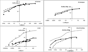
Acuity is a well-established metric for describing the upper limit of spatial vision. It has often been determined using square-wave gratings with a fixed high contrast (Michelson contrast near or at unity). With the use of gratings, the spatial frequency (expressed in c/deg) at the threshold of structure detection is given as a measure of acuity. The data points given in Fig. 2a–2d show acuity values determined from the measured CSF data given for the macaque (De Valois et al., Reference De Valois, Morgan and Snodderley1974), cat (Pasternak & Merigan, Reference Pasternak and Merigan1981), owl monkey (Jacobs, Reference Jacobs1977), and the human. For the latter, CSF data were obtained from three sources; van Meeteren and Vos (Reference van Meeteren and Vos1972), Ghim (Reference Ghim1997), and DePalma and Lowry (Reference DePalma and Lowry1962). The cat data are also supplemented with acuity values calculated from the CSF studies provided by Blake et al. (Reference Blake, Cool and Crawford1974), Bisti and Maffei (Reference Bisti and Maffei1974), Kang et al. (Reference Kang, Reem, Kaczmarowski and Malpeli2009), and calculated acuity from Gianfranceschi et al. (Reference Gianfranceschi, Fiorentini and Maffei1999). For each species, Fig. 2 shows the change in acuity as stimulus luminance decreases from photopic down to scotopic levels. The solid line in each plot gives theoretical acuity calculated from eqn. (1) using either photopic or scotopic parameter values as appropriate. For a given luminance, this theoretical acuity is given by the high frequency value of u (c/deg) when S(u) equals 1.0. The extended hatch curves in Fig. 2 represent theoretical acuity if the photopic model is used at scotopic levels and shows for both primates (Fig. 2a and 2b) an overestimation of acuity at low luminance levels. For the two nocturnal species (Fig. 2c and 2d), the reverse case occurs. In all four vertebrates examined, the appropriate switch from photopic to scotopic parameter values establishes a good fit between modeled and measured acuity at all luminances.
Acuity (c/deg) versus stimulus luminance (cd/m2). Hatch curve; theoretical result calculated from eqn. (1) with photopic parameter values. Data points; measured values. Solid curve; theoretical values calculated with scotopic or photopic parameter values as appropriate. (a) Result for the human. Circles; from van Meeteren and Vos (Reference van Meeteren and Vos1972). Squares; Ghim (Reference Ghim1997). Triangles; DePalma and Lowry (Reference DePalma and Lowry1962). (b) Result for macaque. Circles; De Valois et al. (Reference De Valois, Morgan and Snodderley1974). (c) Result for cat. Open circle; Blake et al. (Reference Blake, Cool and Crawford1974). Circles; Pasternak and Merigan (Reference Pasternak and Merigan1981). Diamonds; Kang et al. (Reference Kang, Reem, Kaczmarowski and Malpeli2009). Square; Bisti and Maffei (Reference Bisti and Maffei1974). Triangle; Gianfranceschi et al. (Reference Gianfranceschi, Fiorentini and Maffei1999). Crosses; human acuity from Pasternak and Merigan (Reference Pasternak and Merigan1981). All data from Pasternak study have been scaled by a factor of 1.8. (d) Results for owl monkey. Circles; Jacobs (Reference Jacobs1977). In (b–d), the human modeled scotopic response is shown as a dotted curve to facilitate a performance comparison.

In Fig. 2c, the human CSF data measured in the Pasternak and Merigan study are also shown, and these have been scaled by a factor of 1.8 to correlate with the human modeled response (uppermost curve). The cat acuity measurements provided by Pasternak and Merigan have also been scaled by a factor of 1.8, and it is significant to note that they now fit on the theoretical trend and align well with the directly measured acuity data provided in the other two cat studies. Some rescaling of the Pasternak and Merigan acuity data would be expected since these authors employed a grating modulation of 0.55 in their experimentation instead of a more suitable value near unity. This would lead to a lower estimation of acuity in terms of c/deg.
Discussion
MTF-based theory for the photopic spatial CSF can be used under scotopic free viewing conditions, provided allowance is made for changes in signal processing incurred with off-axis imaging and with rod photoreception. The validation of this theoretical approach was achieved using measured CSF data for two vertebrate visual systems, which are suited for diurnal conditions and two suited for nocturnal conditions. In all four species studied (the human, macaque, cat, and owl monkey), an acceptable fit was found between theoretical and measured CSF.
Our analyses divide the visual mechanisms controlling the CSF into photon capture and management factors, which are then followed by neural elements. In terms of the initial capture of light, dilation in pupil size at low light luminance operates to increase retinal illuminance, which lowers photon noise. A larger pupil size also lowers the optical MTF, which, in turn, reduces high frequency CSF and acuity. Direct double-pass light probe determinations of the optical MTF have been made in a range of species including the human (Campbell & Gubisch, Reference Campbell and Gubisch1966), chicken (Coletta et al., Reference Coletta, Marcos, Wildsoet and Troilo2003), cat (Bonds, Reference Bonds1974), and rat (Artal et al., Reference Artal, Herreros De Tejada, Munoz Tedo and Green1998). All indicate a reduction in the optical MTF as pupil size increases.
The important changes in both optical and neural mechanisms subserving the CSF as conditions move from photopic to scotopic can be deduced from the numerical parameter values given in Table 1. The quantum efficiency, for example, of both cat and owl monkey increases considerably under scotopic conditions due to the relatively high density of rods in both species. This increase is particularly large in the owl monkey being around 20-fold. The reverse is the case in both the human and macaque, where quantum efficiency decreases slightly under scotopic conditions.
The difference in behavior of quantum efficiency shown by visual systems favoring nocturnal conditions compared with systems favoring diurnal conditions at low luminance has a profound effect on spatial vision. For example, the acuity curves of Fig. 2 illustrate that in both the human and macaque, a switch from photopic to scotopic conditions induces an increase in the rate of acuity loss. The reverse is true with the cat and owl monkey (nocturnal) and this is primarily due to the difference in the behavior of quantum efficiency. This improvement in the sustainability of acuity in the cat and owl monkey indicates that although overall photopic spatial vision in these species is relatively poor compared with the human and macaque, the perceptual change in going from daylight to night conditions will not be as dramatic in a perceptual sense; a factor likely to have an important bearing on patterns of behavior in the natural environment. This sustainability produces an acuity approaching that of the human at low luminance (see Fig. 2c and 2d). There is some evidence from a second experiment performed with 80% modulation square-wave gratings with the owl monkey (Jacobs, Reference Jacobs1977) that low luminance acuity in this species may even surpass that of the human.
Our analysis, therefore, indicates that the transition from cone to rod vision has opposite effects on quantum efficiency in different species and it is this mechanism, which strongly dictates observed differences in CSF at low luminance. Unfortunately, over the years, direct studies of human quantum efficiency (and its constituent parts) have produced widely varying estimates, and this is due in part to differences in experimental methodology. In his early work, Barlow (Reference Barlow1962) derives a figure of 5% for highest overall quantum efficiency in human vision but then later concludes it must be in the range 11–33% for rods (Barlow, Reference Barlow, Barlow and Fatt1977). These second figures were obtained by cascading together all photon capture events from media transmission to fraction exciting some response. Pelli (Reference Pelli and Blakemore1990) offers a thorough review and critique of the subject and finally defines overall quantum efficiency as a product of transduction efficiency and calculation efficiency. As outlined in the Theoretical framework section, quantum efficiency in the Barten theory is strictly speaking the transduction efficiency component described by Pelli. From a study of transduction efficiency determinations obtained from Nagaraja (Reference Nagaraja1964), van Meeteren (Reference van Meeteren1973), van Meeteren and Boogaard (Reference van Meeteren and Boogaard1973), and Pelli (Reference Pelli1983), Pelli concludes that this efficiency term has a range of 1–3%. Clearly, we are faced with a wide range of values if we historically review all results but make the assumption that the Pelli figures for transduction efficiency are appropriate in our modeling.
A review of Table 1 also shows that changes in the neural parameters X max, R max, σ, and N it are qualitatively the same for the human, owl monkey, and the cat as conditions change from photopic to scotopic. This finding is consistent with conclusions made by Kang et al. (Reference Kang, Reem, Kaczmarowski and Malpeli2009) on neural processing factors in their recent study of cat and human CSF. In all four species studied, the only neural mechanism which functions to enhance sensitivity at low luminance is the increase in retinal area over which spatial summation occurs (an increase in parameter X max). Our analysis of the owl monkey visual system indicates that no significant change in any of the neural mechanisms underlying the spatial CSF are incurred at low luminance, due to the use of central viewing by this animal.
In general, a reduction in stimulus luminance leads to a more low-pass characteristic for the CSF, which traditionally has been explained as reflecting a reduction in lateral inhibition. The Barten model predicts this behavior through increasing levels of photon noise as luminance decreases. Under these conditions, total system noise N [see eqn. 3] tends toward  . The lateral inhibition term H which controls the band-pass behavior of the CSF cancels out in the main model expression [eqn (1)]. This loss in lateral inhibition is consistent with recent theoretical studies of the role played by the retina in improving signal/noise ratio at low luminances (Graham et al., Reference Graham, Chandler and Field2006). Makous (Reference Makous, Werner and Chalupa2004) also emphasizes the importance of improved signal/noise; the rod system may enhance relatively low signal/noise ratios in small areas of the retina under scotopic conditions, by averaging the signal over larger areas than the cone system can achieve. Certainly, ganglion cell receptive field centers increase with increasing eccentricity (Peichl & Wassle, Reference Peichl and Wassle1979)
An important question is how does this analysis relating to lateral inhibition at low luminance stand against knowledge obtained from direct electrophysiology? Early classic work on the cat retina (Barlow et al., Reference Barlow, Fitzhugh and Kuffler1957; Enroth-Cugell & Lennie, Reference Enroth-Cugell and Lennie1975) shows a reduction or complete loss in lateral inhibition in ganglion cell field surround response with dark adaptation. Similar findings were obtained Kaplan et al. (Reference Kaplan, Marcus and So1979) in their study of receptive field behavior at both ganglion cell and lateral geniculate nucleus levels in the cat. Of interest is that these authors, working with both P- and M-pathway cells, found that receptive field centers expanded as luminance level reduced. At the lowest light level examined (0.012 cd/m2), field centers tended to expand to the entire surround width. Such an expansion could be operating to improve the signal gain that Makous describes. Whether or not this dynamic change in receptive field center size is simply leading to a masking of the lateral inhibition mechanism, or the surround inhibitory mechanism per se is actually reduced in strength at low luminance is simply not clear. The exact mechanism behind the apparent weakening of lateral inhibition in retinal ganglion cells with dark adaptation still remains to some extent, a controversial issue.
An enlargement of ganglion cell receptive field centers could also theoretically operate to reduce high frequency CSF, acting in addition to optical light spreading. Although both optical spread and receptor sampling are incorporated in the Barten model to allow for early signal attenuation, no term relating to ganglion field expansion exists in the re-engineered model for scotopic CSF. At present, there is insufficient data available on field center expansion, to incorporate this factor in the Barten theory for vertebrate spatial CSF in general.
Appendix 1
The Rovamo–Barten MTF model for photopic spatial CSF
The Rovamo–Barten model has two variants; one as defined by Barten and the other by Rovamo et al. Although both variants are represented by eqn. (1) in the main text, each expresses the functional form of O, H, A, and the constant K in this equation in a slightly different way. It is therefore important to examine and analyze these differences and this is carried out in sections below.
As given in the main text [eqn. (3)], the total system (contrast) noise (N) is defined (in both Barten and Rovamo variants of the model) as:

Eqn. (A.1) shows that the total noise is considered partly due to noise generated by the statistical fluctuations in the number of incident photons and partly due to neural noise caused by statistical fluctuations in the signal passing through to the cortex. Photon noise is not filtered by eye optics but by the lateral inhibition process. This noise component is also inversely proportional to the average photon flux density (Rose, Reference Rose1948). Expressed in terms of retinal illuminance (I Td), Barten obtains the expression  , where η is the quantum efficiency of the eye defined as the ratio of the number of photons causing excitation of the photoreceptors to the number entering the eye; it is therefore equivalent to transduction efficiency as defined by Pelli (Reference Pelli and Blakemore1990). In human vision, studies of quantum efficiency have produced a wide range of values as discussed in the main text. The study of Pelli (Reference Pelli and Blakemore1990) reviews these, and the conclusion drawn is that the transduction component in overall visual quantum efficiency must lie in the range 0.01–0.03. The factor ρ is a photon conversion factor and for most light sources is approximately 1.2 × 10⁶ photons/s/deg2/Td (Scheibner & Baumgardt, Reference Scheibner and Baumgardt1967; Barten, Reference Barten1999). Rovamo et al. define the photon noise term as
 and state that (N qt)−1 is the effective luminous flux absorbed by the photoreceptors rather than the input luminous flux. The basic proportionality constant in the Rovamo definition of N qt will thus contain a quantum efficiency term as in the Barten variant. That a quantum efficiency term exists in the Rovamo model variant is not, however, obvious in the mathematical treatment given. At moderate to high levels of light, N qt becomes negligible and the overall system noise defined by the neural noise N it.
Analysis of Functions O, H, and A
In the Rovamo et al. modeling, O does not incorporate a term accounting for retinal sampling. The Barten treatment, however, rectifies this omission and defines O as a cascade of the OMTF with the MTF representing the retinal sampling process (MTFr). Thus according to Barten:

From our previous studies of eqn. (A.2) (Jarvis & Wathes, Reference Jarvis and Wathes2007), the functional form of OMTF can be represented by a Butterworth function given by,

where u * represents the spatial frequency when OMTF reaches a value of 0.5. Eqn. (A.3) is also used by Rovamo et al. but as a representation of function O. Mathematically, eqn. (A.3) behaves in a similar fashion to the Deeley function (Deeley et al., Reference Deeley, Drasdo and Charman1991), which provides realistic estimates for the human OMTF as a function of pupil diameter. From a consideration of ganglion cell spacing in the retina, MTFr can be represented by a Gaussian function (Barten, Reference Barten1999; Jarvis & Wathes, Reference Jarvis and Wathes2007). Thus,

The parameter σ in eqn. (A.4) is the standard deviation of the ganglion cell sampling line spread function.
The lateral inhibition term H is defined by Barten as:

where the parameter u 0 is the spatial frequency value above which the effect of lateral inhibition ceases. Eqn. (A.5) represents the action of a high-pass filtering process and is consistent with the lateral inhibition MTF derived by Donner and Hemila (Reference Donner and Hemila1996) for vertebrate vision. In the Rovamo et al. model variant, H is revealed as directly proportional to u. This definition of an MTF representing what is essentially a negative feedback mechanism is not theoretically tenable. Eqn. (A.5) represents a function that saturates to unity, which is a feature of an MTF representing this type of filtering mechanism whether in a biological (Donner & Hemila, Reference Donner and Hemila1996), electronic (Castleman, Reference Castleman1996), or chemical (Jarvis, Reference Jarvis1994) imaging system.
The area function A represents an integration stage of spatial information processed forward to the cortex from the retina. Barten derives the following expression for A:

where X max represents the upper angular size limit (deg) over which a visual system can integrate spatial information. There is also an upper limit of the spatial integration capacity formed by a maximum number of cycles R max. The angular size (deg) of the grating stimulus is represented by X 0. Eqn. (A.6) was derived by Barten partly through analogy to the temporal expression given by Schade (Reference Schade1956) relating the integration time of the eye to stimulus duration. The inclusion of the term R max, however, originates simply from an examination of experimental studies of the relationship between contrast sensitivity and number of cycles contained within a grating stimulus. In the Rovamo et al. model variant, A becomes

where A 0 represents the maximum area over which the visual system can integrate information and is equivalent to Barten’s term  in eqn. (A.6). The spatial frequency uc is equivalent to Barten’s term R max. As in the Barten model variant, eqn. (A.7) is derived from experimental measurements determined with a variable grating size. The two equations are not, however, algebraically equivalent. At photopic light levels, both Barten and Rovamo et al. versions of eqn. (1) in the main text do provide good models for the general shape of the measured human CSF. That both model variants can achieve this is due to the fact that the function product (
 ) has a similar mathematical form even though the component functions differ.
Analysis of the constant K
The basic constant K in eqn. (1) of the main text differs between the Barten and Rovamo et al. model variants. According to Barten, K is given by,

where T is the overall integration time of the eye and 1/k is the Crozier coefficient, a basic signal/noise constant for the detection of a luminance signal with a value for human vision of about 0.3 (Roufs, Reference Roufs1974). In eqn. (A.8), K is numerically defined for binocular viewing conditions. Its value for monocular viewing conditions is lower by a factor ( ). Eqn. (A.8) was derived from a consideration of the way both image noise and the basic visual psychometric function impact on contrast sensitivity (Barten, Reference Barten1999). For the human, Barten defines a value of 0.1 s for T using the photoelectric model of the eye proposed by Schade (Reference Schade1956).
In the Rovamo et al. model variant, K (for monocular viewing) is given by:

where d is the detectability index. This term, which was first employed in acoustical studies (Tanner & Birdsall, Reference Tanner and Birdsall1958), is used by Rovamo et al. in the definition of the signal/noise performance in an idealized detection filter. The performance of this filter, when directly compared with that of a theoretical human system, is used in the development of the model. The term μ donates the maximum efficiency of the human detection filter. The conceptualization of K is thus different between the two model variants. The Barten definition stems from a consideration of near threshold contrast discrimination ability (as defined through the psychometric function) together with overall integration time for the eye. The Rovamo et al. definition stems from a comparison between idealized and human detection filters. Even though this fundamental difference exists in the detailed interpretation of K, both definitions provide a single-valued factor whose magnitude defines a measure of the efficiency of a basic signal detection mechanism in the cortex.
In the evaluation of vertebrate CSF given in the main text, we choose the Barten variant of the model mainly because of the more realistic mathematical interpretation of lateral inhibition. Through Hankel transformation, the lateral inhibition MTF gives an estimate of ganglion cell receptive field surround size, and previous estimates of these field sizes from vertebrate CSF data have correlated well with direct estimates made through electrophysiology in a range of species (Jarvis & Wathes, Reference Jarvis and Wathes2008). Our choice of the Barten mathematics is also due in part, to the inclusion of an MTF term quantifying receptor sampling, although this could be theoretically incorporated in the Rovamo et al. variant.
Calculating Barten model parameters
The Barten model variant contains eight parameters, the values of which will be specific to a given species. In summary, these are (with functional significance shown in parentheses); K (detection), u * (optics), σ (retinal sampling), η (quantum efficiency), u 0 (lateral inhibition), X max, R max (summation limits), and N it (neural noise). As shown above, values for both K and η can be specified for human vision.
In the application of the model to measured human contrast sensitivity data, Barten derived parameter values from a “trial and error” curve fitting process. Nevertheless, having established numerical values from a limited data source, the model was found to provide good predictions of contrast sensitivity measured for an extensive range of stimulus conditions (Barten Reference Barten1999). It is, however, possible to calculate the model parameter values because the mathematical form of the model can be simplified algebraically within specific spatial frequency bands. Theoretically, this applies to any species, and the mathematical procedures required are now described. In the following analysis, low frequency refers to spatial frequencies less than that for maximum contrast sensitivity in a given species and high frequency to spatial frequencies greater than that for maximum contrast sensitivity.
Evaluation of parameters u* and σ
It was shown in a previous publication (Jarvis & Wathes, Reference Jarvis and Wathes2007) that if OMTF is defined as a Butterworth function [eqn. (A.3)], the model at high frequencies reduces to the simple form,

Thus providing the retinal sampling response MTFr is known, eqn. (A.10) can be used to directly estimate the optical response parameter u * from measured values of S at high frequency. The parameter σ defines MTFr and can be calculated from ganglion cell density data (Jarvis & Wathes, Reference Jarvis and Wathes2007). Eqn. (A.10) has already been tested on a range of vertebrates and found to describe optical performance similar to that derived from direct double-pass measurements. Full details of the application and testing of eqn. (A.10) are given elsewhere (Jarvis & Wathes, Reference Jarvis and Wathes2007).
Evaluation of parameter Xmax
This parameter can be calculated from contrast sensitivity data measured with two sizes of grating at a similar luminance. An inspection of eqn. (A.6) shows that at a given low frequency, the value of A is determined by both X 0 and X max since the u 2 term tends toward zero. An increase in grating size X 0 leads to an increase in the value of A and as a consequence contrast sensitivity S [eqn. (1)]. At high spatial frequency, eqn. (A.6) indicates that changing grating size should have little effect on contrast sensitivity because now the value of A is controlled by the term ( ). Let
 and
 be measured contrast sensitivity at a given low frequency with two grating sizes X 1 and X 2, where X 1 > X 2. At a given low frequency, the model gives,

or,

The second term on the right-hand side of eqn. (A.12) defines the increase in log(S) when grating size increases from X 2 to X 1. It represents a proportional increase, which is the same at any given low spatial frequency. Parameter X max can be calculated from this increase since X 1 and X 2 are known from the experimental design. The predicted behavior of S as grating size changes is observed in measured data for all species examined in our previous detailed study (Jarvis & Wathes, Reference Jarvis and Wathes2008).
Evaluation of parameter u0
The lateral inhibition parameter u 0 can be evaluated from low frequency contrast sensitivity data obtained from a high luminance grating stimulus. For these conditions, the function O in eqn. (1) tends toward unity (Jarvis & Wathes, Reference Jarvis and Wathes2007) and photon noise as defined through eqn. (4) in the main text becomes negligible. The model then predicts for these conditions,

where ķ is given by,

Neural noise N it is considered to be white (N it(u) = N it(0)) and so ķ is a frequency-independent constant. As for eqn. (A.12), the validity of eqn. (A.13) has been tested by applying it to measured high luminance CSF data for a range of species (Jarvis & Wathes, Reference Jarvis and Wathes2008). The predicted behavior of S 2 as a function of spatial frequency was observed with measured data in all species studied, and a simple curve fitting procedure revealed the numerical value of parameter u 0. The constant ķ can also be obtained from the curve fitting procedure, and since X max is now known, eqn. (A.13) directly yields a numerical value for the ratio (K 2/N it).
Evaluation of parameters Nit and η
Contrast sensitivity data obtained at two luminance levels can be employed to test the model and estimate these parameters. Let I 1 and I 2 (I 1 > I 2) be the retinal illuminance values associated with the two mean grating luminance levels and SI 1 and SI 2 be the corresponding contrast sensitivity values at a given spatial frequency. If frequency is high, the function H [see eqn. (A.5)] is unity and the model equations predict,

where,

The OMTF terms in eqn. (A.16) are values associated with the two luminance levels. The photon noise terms ( and
 ) in eqn. (A.15) require values of quantum efficiency (η) to be known for a given species. This can theoretically be overcome by defining the new mathematical parameter (ηN it). Thus, rearranging terms in eqn. (A.15) gives,

In eqn. (A.17), both I1 and I2 can be calculated from stimulus luminance providing the PND and pupil size for the species are known (Hughes, Reference Hughes and Crescitelli1977). Combining measured values of S 2 with calculated values of I yields ηN it. The model predicts that eqn. (A.17) becomes a constant (the value of ηN it) at high spatial frequencies.
Analysis of factor K
As shown in section above, quantum efficiency η was removed from the photon noise term in order to facilitate the analysis using eqn. (A.15). To employ the model in a practical sense for the specification of contrast sensitivity at all frequencies, a similar modification must be made to eqn. (A.1). This is simply facilitated by the replacement of N it with (ηN it) in this equation. The algebraic consequence of this modification is that the factor K in the complete model given by eqn. (1) in the main text is replaced by the product ( ). This modification is mathematically trivial, but as shown above, the use of the new parameter (ηN it) avoids the necessity of directly calculating quantum efficiency. The determination of (ηN it) allows the system detection efficiency term (
 ) to be evaluated. Since both (K 2/N it) and (ηN it) can be calculated for a given species (as shown in sections above), the value of (
 ) follows immediately.
Evaluation of parameter Rmax
The final parameter for evaluation is the limiting number of cycles term R max given in eqn. (A.8). This can be directly calculated from high frequency contrast sensitivity data. At high frequencies, the function H becomes unity and the function A approaches the value ( ). For these conditions, the model gives,

Rearranging terms in eqn. (A.18) gives,

The model therefore predicts that values of  will saturate at the level given by the right-hand side of eqn. (A.19) at high frequency. The value of the saturation asymptote yields a numerical value R max since all other parameters have now been calculated.
Using directly measured CSF data from a range of species, including the human, the mathematical predictions given by eqns. (A.12), (A.13), (A.17), and (A.19) have been shown to occur as outlined in our previous study of vertebrate CSF (Jarvis & Wathes, Reference Jarvis and Wathes2008). In this study, we also compare the algebraic techniques for parameter estimation given above with a nonlinear curve fitting algorithm. This was seen to produce comparable parameter estimations, and full details of this accuracy examination are given in the publication referenced above.
Appendix 2
Calculation of scotopic model parameter values
Numerical values for the scotopic parameters outlined in the Theoretical framework section were calculated as given below. The analysis is shown separately for each species; since by necessity, the calculation methodology differed slightly with the cat and owl monkey. The calculation of some scotopic parameter values requires photopic values to be known.
Human model parameters
σ(e) (retinal sampling): As outlined in Appendix 1, signal loss due to retinal sampling is described by MTFr, which is numerically defined through a single parameter σ relating to ganglion cell density. For scotopic vision, ganglion cell density at 10-deg eccentricity is appropriate and a figure of 500 cells/deg2 was taken (Curcio & Allen, Reference Curcio and Allen1990). From this figure, σ(e) was calculated to be 0.76 arcmin.
η(e), N it(e) (quantum efficiency and internal neural noise): Over the retinal illuminance range 0.001–100 Td, human quantum efficiency varies from around 0.015 to 0.03 (Pelli, Reference Pelli and Blakemore1990). Under photopic conditions, the parameter product  is already known (Jarvis & Wathes, Reference Jarvis and Wathes2008) and has the value 9.0 × 10⁻¹⁰ s deg2. If η(c) is taken to be 0.03, as suggested by Barten, then photopic internal neural noise N it(c) is 3.0 × 10⁻⁸ s deg2. Using data from Curcio & Allen (Reference Curcio and Allen1990), Barten estimates that at an eccentricity of 10 deg, ganglion cell density is 0.016 times that in the fovea. The above values give, through eqn. (5) in the main text, a value of 200.0 × 10⁻⁸ s deg2 for N it(e). Pelli's analysis gives a value of 0.015 for η(e), which provides an estimate of 3.0 × 10⁻⁸ s deg2 for the product η(e).N it(e) in human vision.
u *(e) (optical attenuation): This parameter defines the optical MTF component in the model (OMTF). The human Deeley function (Deeley et al., Reference Deeley, Drasdo and Charman1991) was used to calculate values for this parameter at the two luminance levels of interest (0.01 and 0.001 cd/m2). At these two luminances, the Deeley OMTF half-height frequency values (which defines u *(e)) are 4.0 and 3.5 c/deg, respectively, and these values were deployed in the model.
uo(e), X max(e), and R max(e) (lateral inhibition and spatial summation): The lateral inhibition parameter (u 0(e)) was calculated from eqn. (6) and the spatial parameter X max(e) from eqn. (7). As argued in the Theoretical framework section, the appropriate value for R max(e) was taken to be 0.5 times its photopic equivalent.
Macaque model parameters
σ(e), η(e), and N it(e): Values of the photopic equivalents of these parameters are similar for both the human and macaque (Jarvis & Wathes, Reference Jarvis and Wathes2008). This is a direct consequence of the two species having similar photoreceptor topography (Goodchild et al., Reference Goodchild, Ghosh and Martin1996). As a consequence, human scotopic values were used in the model calculations.
u *(e): Values of the optical parameter were estimated to be 8.0 and 7.0 c/deg from double-pass data obtained in this species by Williams and Boothe (Reference Williams and Boothe1981). The remaining scotopic model parameters were calculated in an identical fashion to those for the human.
Cat model parameters
σ(e): This parameter was calculated to be 2.46 arcmin using ganglion cell density data from Stone (Reference Stone1965).
η(e) and N it(e): Rod density is higher in the cat compared with the human and a study of retinal performance at low luminance gives η(e) to be about 2.7 times greater than the human value (Bonds & MacLeod, Reference Bonds and MacLeod1974). This suggests a figure of around 0.04 for η(e). Under photopic conditions, η(c) will be enhanced by a factor of about 1.6 compared with the human due to the tapetum lucidum (Berkley, 1975) and decreased due to there being approximately 10 times fewer cones (Steinberg et al., Reference Steinberg, Reid and Lacy1973). This would suggest that a reasonable estimate for the photopic quantum efficiency η(c) in the cat is 0.0048.
An analysis of the Pasternak and Merigan photopic CSF data gives a value of 4.0 × 10⁻⁹ s deg2 for  and so it follows immediately that N it(c) is equal to 8.33 × 10⁻⁷ s deg2. From the data provided by Stone (Reference Stone1965), we estimate that at an eccentricity of 10 deg, ganglion cell density is approximately 7.0 times less than that in the central fovea. From this, eqn. (5) gives a value of 5.83 × 10⁻⁶ s deg2 for N it(e) in the cat.
u *(e): Values for the optical parameter were determined from the double-pass data provided by Bonds (Reference Bonds1974). Under the experimental conditions used by Pasternak and Merigan (Reference Pasternak and Merigan1981), pupil diameter is close to maximum (12 mm) and the double-pass optical data of Bonds (Reference Bonds1974) give a value of 1.4 c/deg for each of the two luminance levels.
u 0(e), X max(e), and R max(e): Again, these parameters were calculated from the already determined photopic values and using the appropriate equations given in the Theoretical framework section. It is of interest to note that at 10-deg eccentricity, eqn. (7) gives a value of just over 2.2 for the ratio of X max(e) and X max(c). Direct measurements of cat CSF for a range of eccentricities (Pasternak & Horn, Reference Pasternak and Horn1991) suggest that this ratio is around 1.5 at 8 deg and 3.8 at 16 deg, in good agreement with the predictions of eqn. (7).
Owl monkey model parameters
With central vision assumed for this species (e = c), scotopic parameter estimations become simplified.
σ(e), η(e), and N it(e): The retinal sampling parameter σ(e) was calculated from the ganglion cell density data provided by Yamada et al. (Reference Yamada, Silveira, Perry and Franco2001). An evaluation of  from the photopic CSF data presented by Jacobs (Reference Jacobs1977) gave a value 4.0 × 10⁻⁹ s deg2 for this parameter product and thus the scotopic product. A value of 0.012 was taken for η(e) since maximum rod density in the owl monkey is around 0.8 times that in the human (Hughes, Reference Hughes and Crescitelli1977). Note also that the Hughes receptor data also reveal that maximum cone density in the owl monkey is 0.017 times that in the human, giving a value for η(c) of 0.0005. If scotopic grating detection is facilitated through central vision in the owl monkey, then N it(e) equals N it(c), that is, 8.0 × 10⁻⁶ s deg2.
u *(e): Values of the optical parameter u * had to be estimated directly from the high frequency CSF data because no directly measured optical response data are available for the owl monkey. These estimates are 2.0 and 1.09 c/deg. All other parameter values were calculated from photopic CSF data provided by Jacobs (Reference Jacobs1977).
Acknowledgments
This work was funded by the Biotechnology and Biological Sciences Research Council under grant BB/C5189221.