I. INTRODUCTION
Ferritic heat-resistant 9–12% Cr steels, due to their good high-temperature endurance, good creep resistance properties, excellent heat conductivity, low thermal expansion coefficient, and high performance-cost ratio, have been considered as the main materials for power plant operating in supercritical or ultra-supercritical conditions.Reference Abe1,Reference Ning, Shi, Yan, Fu, Liu and Bie2 In these steels, M23C6 is an important kind of precipitate during tempering, whose particle size and dispersivity are essential ingredients for the high performance of these steels as these metallic carbide precipitates exert strong pinning forces on dislocations and subgrains.Reference Singhal and Martin3–Reference Abe, Taneike and Sawada5 Thus, it is imperative to develop a kinetics model to predict the precipitation of M23C6 in these steels.
As is well known, the kinetics for a transformation involves nucleation, growth, and impingement.Reference Liu, Sommer and Mittemeijer6,Reference Liu, Nitsche, Sommer and Mittemeijer7 Generally, there are two kinds of impingements, i.e., hard-impingement considering geometrical factor, and soft-impingement considering the overlap of diffusion fields. When considering the hard-impingement, a classic Johnson-Mehl-Avrami (JMA) model can be built to describe a large number of different solid phase transformations.Reference Ruitenberg, Woldt and Petford-Long8,Reference Starink and Zahra9 In this way, Jones, Robson, and Bhadeshia built a modified JMA model to describe the overall transformation kinetics of the precipitation in power plant steels even with simultaneous occurrence of two or more transformations.Reference Robson and Bhadeshia10,Reference Robson and Bhadeshia11 However, soft-impingement has been found to prevail in the solid-state transformations especially the diffusion-controlled reaction.Reference Liu, Sommer, Bos and Mittemeijer12 The process of soft-impingement consists of two stages. During the early stage of soft-impingement, the overlap of diffusion fields occurs only in a limited number of directions, resulting in the different concentration gradients of solute in different directions around the particle. And during the late stage, the diffusion fields are approximately the same in all directions around the particle. However, the early stage of soft-impingement has a short duration and can be ignored in view of the large nucleation density and the fast diffusion of solute atoms.Reference Offerman, Van Dijk, Sietsma, Lauridsen, Margulies, Grigull, Poulsen and Van Der Zwaag13,Reference Chen and van der Zwaag14 Gilmour et al.Reference Gilmour, Purdy and Kirkaldy15,Reference Gilmour, Purdy and Kirkaldy16 have shown that their soft-impingement model is in reasonable agreement with experimental evidence on Fe–Mn–C alloys. Bhadeshia et al. have found an equation that can be used to treat soft-impingement in Fe–C alloys by making appropriate substitutions for the various concentration terms.Reference Bhadeshia17 Andres et al. built a model to describe the growth kinetics of isothermal ferrite formation in a medium-carbon microalloyed steel, in which the effect of soft-impingement has been dealt with based on work by Gilmour et al.Reference Andres, Capdevila, Caballero and Bhadeshia18 Ge. Yu et al.Reference Yu, Lai and Zhang19 discussed the effect of overlapping diffusion zones by numerically solving the diffusion function for the model systems. Yet, the models mentioned above are either empirical in nature or inconvenient to generalize the effects of soft impingement on precipitations, i.e., a clear relationship between the transformed fraction (f) and time (t) is unavailable. Therefore, an analytical model, which gives a clear f-t relationship on precipitation in the case of 1D and 3D, was developed by Fan et al.Reference Fan, Liu, Liu, Zhang, Yang and Zhou20 based on Ge. Yu et al.Reference Yu, Lai and Zhang19 and the model managed to predict the isothermal ferrite formation in 0.37C–1.45Mn-0.11V microalloyed steel and precipitation in an Al-0.2wt%Sc alloy. However, results from use of this model for predicting the precipitation parameters of M23C6 in heat-resistant steels such as required for critical power plant applications have been found to be inaccurate, due to its temperature-independent growth coefficient, like Zener’s,Reference Zener21 and the absence of 2D case. Therefore, based on the model of Fan, a modified model aimed at accurately describing the precipitation of M23C6 in steels is developed and its parameters are discussed in detail.
II. EXPERIMENTAL PROCEDURES
The experimental material was manufactured by Tianjin Pipe (Group) Corporation and its chemical composition is shown in Table I. To reduce the temperature difference between the bulk and surface of materials to an acceptable level during fast heating and cooling processing, the material was cut into small sheets with a size of 10 × 10 × 0.3 mm. The sheets were austenitized at 1050 °C for 1800 s in vacuum furnace followed by air cooling to room temperature, and then tempered at 650 °C for different time durations ranging from 10 s to 3.6 × 10⁵ s.
Chemical composition of the experimental T/P92 steel (in wt%).

The chemical extraction was conducted using a solution of 15% HCl (vol%). In this condition, the matrix was dissolved, while carbides remained. The mass fraction of M23C6 precipitates was calculated by measuring the mass of the extracted carbides, as all carbides were almost M23C6. The equilibrium chemical composition of M23C6 in T/P92 steel at 650 °C was calculated by Thermo-Calc software with FEDAT TCS\TT Steel database, listed in Table II.
Calculated composition of M23C6.

III. MODEL DERIVATION
A. Nucleation
According to the classical nucleation theory, nucleation is defined as the formation of particles from subcritical size to supercritical size.Reference Mittemeijer22 During nucleation, the production of new phase releases chemical Gibbs energy whereas the creation of the interfaces costs Gibbs energy. Precipitation could be governed by various nucleation modes, including continuous nucleation, site saturation nucleation, and the intermediate nucleation called mixed nucleation or Avrami nucleation.Reference Liu, Sommer, Bos and Mittemeijer12,Reference Avrami23–Reference Avrami25 The nucleation of M23C6 is typically heterogeneous, which occurs along martensite laths or prior austenite grain boundaries. In this case, the interface energy is lower and the critical size is larger than that in homogeneous nucleation. As the nucleation rate decreases drastically with the decline of solute saturation caused by solute redistribution,Reference Fan, Liu, Liu, Zhang, Yang and Zhou20 the nucleation in diffusion-controlled transformation, such as the precipitation of M23C6, is usually assumed to be dominated by site saturation nucleation, which indicates that there already are a number of preexisting nuclei (supercritical particles of the new phase) at t = 0 and the further nucleation rate is zero.Reference Liu, Nitsche, Sommer and Mittemeijer7
B. Growth
Generally, two kinds of growth are considered: volume-diffusion-controlled growth which occurs in phase transformations where long-range compositional changes take place; and interface-diffusion-controlled growth which occurs as the growth is determined by atomic processes at and near the interfaces. The growth of M23C6 is a typical volume-diffusion-controlled one, which is characterized by solute diffusion in the growth front (precipitation/matrix interface). The growth of M23C6 in T/P92 steel can be decelerated arising out of the segregation of substitutional alloying elements such as chromium (Cr), tungsten (W), and molybdenum (Mo)etc.,Reference Chen and van der Zwaag26 at and near the interfaces. The retardation effect had been found in γ-α transformation in ternary Fe–C–M alloys by applying the local equilibrium (LE) model, in which both carbon (C) and M can have partitioning, where M denotes the sum of carbide-forming metal elements.Reference Chen, Appolaire and van der Zwaag27,Reference Chen and van der Zwaag28 However, it is complex to deal with the LE model because there are so many kinds of substitutional alloying elements in this steel. Therefore, this work is based on the assumption that substitutional alloying elements are immobile, i.e., the precipitation of M23C6 is controlled only by the diffusion of C, and the model would possibly overestimate the transformation kinetics, as the segregation of alloying element into interface will cause dissipation of Gibbs energy.
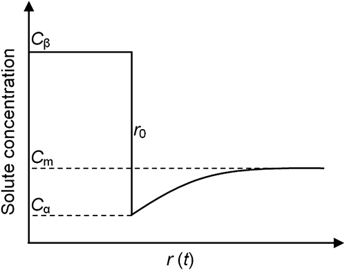
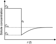
Accordingly, two types of precipitation are classified by the diffusion direction: positive precipitation, where the solution atoms diffuse into the growth front; and negative precipitation, where the solute atoms diffuse away from the moving interface.Reference Zener21 The carbide precipitation in α-Fe is typically positive, the schematic diagram of the diffusion profile is illustrated in Fig. 1, where C β and C α are the equilibrium concentration in the after-transformation precipitate and matrix, respectively, C m is the saturated composition in the nontransformed single phase alloy, and r 0 is the position of the growth front.
Schematic image of diffusion profile in positive precipitation.
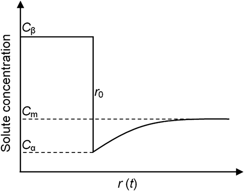
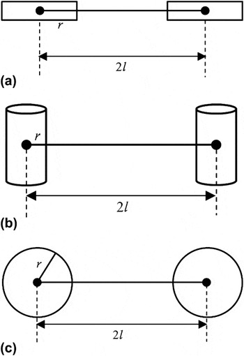
The growth of two adjacent particles is divided into three types by the number of dimensions, as illustrated in Fig. 2. In one-dimensional case, r 0 is the half width of the plate, in two-dimensional case, r 0 is the radius of the cylinder, and in the case of three-dimensional growth, r 0 is the radius of the spherical particle with 2l being the distance of the two particles.
Schematic image of the three kinds of growth mode: (a) 1D case; (b) 2D case; (c) 3D case.

The diffusion of solute atoms can be described by the classical diffusion equation:
 $${{\partial C} \over {\partial t}} = D\nabla ^2 C + \left( {\left( \,{p - 1} \right)\left( {{D \over r}} \right)} \right)\left( {\nabla C} \right)\,\quad,$$
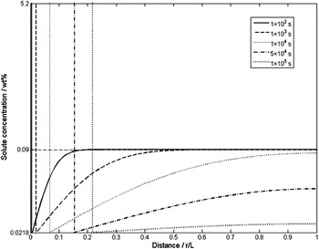
where p equals 1, 2, or 3 for 1D, 2D, and 3D growth, respectively and D is the temperature-dependent diffusion coefficient of solute atoms, which is constant in isothermal transformation. C is the concentration of solute atoms, which varies as a function of the position of growth front r and the transformation time t. Meanwhile, r also varies as a function of time. The numerical solution of Eq. (1) can be obtained under boundary conditions: C(r 0, t) = C α, C(r, 0) = C m and  $\left( {{{\partial C} \mathord{\left/ {\vphantom {{\partial C} {\partial r}}} \right. \kern-\nulldelimiterspace} {\partial r}}} \right)_{r = l} \,\,= 0$, with l representing the position of impingement and being equal to half distance of two adjacent particles. Using this numerical solution and the value of growth coefficient λ (obtained by fitting, see more details in Sec. IV), the real concentration of M23C6 precipitation in steels can be obtained, as shown in Fig. 3. With time prolonging, the position of growth front advances and the slope of concentration curve in front of the interface declines as a function of distance away from the interface. If time duration is sufficiently long, the concentration of solute atoms at r = l is less than C m, suggesting the occurrence of the overlapping of diffusion fields, i.e., the occurrence of soft impingement.
The diffusion profile of M23C6 precipitation in T92 steel, which is obtained by combination of numerical solution of diffusion equation and growth coefficient.

C. Soft impingement model with linear concentration profile
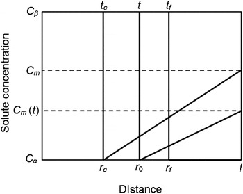
For simplifying the soft impingement model, a linear approximation of concentration profile needs to be conducted. Figure 4 illustrates the linear approximation of the concentration profile in front of the interface and the transition of diffusion fields from nonoverlapping (i.e., nonimpingement) to overlapping (i.e., impingement). r c is the critical particle size in soft impingement. Before impingement, the position of growth front does not reach r c, and the growth of precipitates follows the square root rule.Reference Wert and Zener29 When the position of growth front exceeds r c, soft impingement takes place, and the overlapping of diffusion fields will retard the growth velocity due to the interference between particles. After the occurrence of soft impingement, C m (t) will change from C m to Cα with prolongation of time. When the position of growth front reaches r f, C m (t) equals Cα, and the transformation will cease as a result of the disappearance of supersaturation.
Schematic image of linear approximation of the diffusion profile, where r c is the critical point of impingement, r f is the end point of impingement t c and t f are the time corresponding to r c and r f respectively.

As shown in Fig. 4, the initiation of soft impingement at r = r c can be obtained according to the conservation law of mass requiringReference Fan, Liu, Liu, Zhang, Yang and Zhou20:
 $$r_{\rm{c}} ^{\,\,\,p} \left( {C_{\rm{\beta }} - C_m } \right) = \left( {l^{\,p} - r_{\rm{c}} ^{\,\,\,p} } \right)\left( {{{C_m - C_{\rm{\alpha }} } \over 2}} \right)\quad,$$
where p equals 1, 2, or 3 for 1D, 2D, and 3D growth, respectively. A rearrangement of Eq. (2) gives
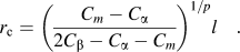 $$r_{\rm{c}} = \left( {{{C_m - C_{\rm{\alpha }} } \over {2C_{\rm{\beta }} - C_{\rm{\alpha }} - C_m }}} \right)^{{1 \mathord{\left/ {\vphantom {1 p}} \right. \kern-\nulldelimiterspace} p}} l\quad.$$
Equation (3) can be used to determine the initial point of soft impingement.
Similarly, the end of transformation at r = r f can also be obtained according to the conservation law of mass requiring:
 $$r_{\rm{f}} ^{\,\,\, p} \left( {C_{\rm{\beta }} - C_m } \right) = \left( {l^{\,p} - r_{\rm{f}} ^{\,\,\,p} } \right)\left( {C_m - C_{\rm{\alpha }} } \right)\,\quad,$$
where p equals 1, 2, or 3 for 1D, 2D, and 3D growth, respectively. And a rearrangement of Eq. (4) gives
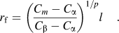 $$r_{\rm{f}} = \left( {{{C_m - C_{\rm{\alpha }} } \over {C_{\rm{\beta }} - C_{\rm{\alpha }} }}} \right)^{{1 \mathord{\left/ {\vphantom {1 p}} \right. \kern-\nulldelimiterspace} p}} l\,\quad.$$
Taking the supersaturation degree as δ = (C m − C α)/(C β − C α) as a reference, Eq. (5) can also be rewritten as:
 $$r_{\rm{f}} = {\rm{\delta }}^{{1 \mathord{\left/ {\vphantom {1 p}} \right. \kern-\nulldelimiterspace} p}} l\,\quad.$$
Thus, Eq. (6) can be used to determine the initial point of soft impingement.
D. Growth before soft impingement
As there is no overlapping of diffusion fields, the growth before soft impingement follows the square root rules, and can be described by Zener’s equationReference Zener21:
 $$r = {\rm{\lambda }}_p \left( {Dt} \right)^{{1 \mathord{\left/ {\vphantom {1 2}} \right. \kern-\nulldelimiterspace} 2}} \,\quad,$$
where λp is the time-independent growth coefficient with p as 1, 2, or 3 for 1D, 2D, and 3D growth. Zener had hypothesized that the growth coefficient λp depended only upon the supersaturation degree δ. However, λp is not a simple function of δ, and it varies from 0 to ∞ as δ varies from 0 to 1. If applied to a complex system, the value of λp would be difficult to obtain.
According to Eq. (7), the initial time of soft impingement t c can be calculated by:
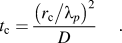 $$t_{\rm{c}} = {{\left( {{{r_{\rm{c}} } \mathord{\left/ {\vphantom {{r_{\rm{c}} } {\lambda _p }}} \right. \kern-\nulldelimiterspace} {\lambda _p }}} \right)^2 } \over D}\,\quad.$$
The transformed fraction f before impingement can be written as:
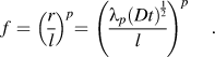 $$f = \left( {{r \over l}} \right)^p = \left( {{{{\rm{\lambda }}_p (Dt)^{{1 \over 2}} } \over l}} \right)^p \quad\,.$$
By substituting and rearranging Eq. (8) into Eq. (10), another form of f can be obtained with r f as a reference:
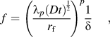 $$f = \left( {{{{\rm{\lambda }}_p (Dt)^{{1 \over 2}} } \over {r_{\rm{f}} }}} \right)^p {1 \over {\rm{\delta }}}\,\quad,$$
where f varies from 0 to 1.
According to Eqs. (3) and (9), the transformed fraction at the initial point of impingement can be given as:
 $$f_{\rm{c}} = \left( {{{r_{\rm{c}} } \over l}} \right)^p = {{C_m - C_{\rm{\alpha }} } \over {2C_{\rm{\beta }} - C_{\rm{\alpha }} - C_m }} = {{\rm{\delta }} \over {2 - {\rm{\delta }}}}\,\quad,$$
suggesting that the transformed fraction at the initial point of impingement depends only on the supersaturation degree δ.
E. Growth after soft impingement
When the position of growth front exceeds r c, i.e., r 0 ≥ r c, soft impingement will take place. The conservation law of mass is still applicable to the determination of r 0:
 $$r_0 ^{\,\,\,p} \left( {C_{\rm{\beta }} - C_m } \right) = \left( {l^{\,p} - r_0 ^{\,\,\,p} } \right)\left( {{{2C_m - C_{\rm{\alpha }} - C_m \left( t \right)} \over 2}} \right)\quad\,.$$
A rearrangement of Eq. (12) gives:
 $$r_0 = \left( {{{2C_m - C_{\rm{\alpha }} - C_m \left( t \right)} \over {2C_{\rm{\beta }} - C_{\rm{\alpha }} - C_m \left( t \right)}}} \right)^{{1 \mathord{\left/ {\vphantom {1 p}} \right. \kern-\nulldelimiterspace} p}} l\,\quad,$$
where C m (t) is a complex function of time. However, Fan et al.Reference Fan, Liu, Liu, Zhang, Yang and Zhou20 have developed the expression for C m (t). Thus if we take r f as a reference, the transformed fraction f after soft impingement can be given as:
 $$f = 1 - \left( {1 - \left( {{{r_{\rm{c}} } \over {r_{\rm{f}} }}} \right)^p } \right)\exp \left( { - k\left( {t - t_{\rm{c}} } \right)} \right)\,\quad,$$
where  $k = \left( {{\textstyle{{pD} \over 2}}} \right)\left( {{\textstyle{{{\rm{\lambda }}_p } \over {r_{\rm{f}} }}}} \right)^p \left( {Dt_1 } \right)^{{{\left( {p - 2} \right)} \over 2}} \left( {1 - \left( {{\textstyle{{r_{\rm{c}} } \over {r_{\rm{f}} }}}} \right)^p } \right)^{ - 1}\quad.$
F. Transformed fraction of the entire transformation
With the combination of Eqs. (10) and (14), the model of transformed fraction as a function of time during the whole transformation process can be written as a piecewise function:
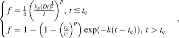 $$\!\!\!\left\{ \matrix{ f = {1 \over {\rm{\delta }}}\left( {{{{\rm{\lambda }}_p (Dt)^{{1 \over 2}} } \over l}} \right)^p ,\,{\rm{ }}t \,\le\, t_{\rm{c}} \hfill \cr f = 1 - \left( {1 - \left( {{{r_{\rm{c}} } \over {r_{\rm{f}} }}} \right)^p } \right)\exp \left( { - k\left( {t - t_{\rm{c}} } \right)} \right),\,{\rm{ }}t > t_{\rm{c}} \hfill \cr} \right.\,\quad,$$
where  $k = \left( {{\textstyle{{pD} \over 2}}} \right)\left( {{\textstyle{{{\rm{\lambda }}_p } \over {r_{\rm{f}} }}}} \right)^p \left( {Dt_1 } \right)^{{{\left( {p - 2} \right)} \over 2}} \left( {1 - \left( {{\textstyle{{r_{\rm{c}} } \over {r_{\rm{f}} }}}} \right)^p } \right)^{ - 1}$, and f varies from 0 to1.
IV. MODEL APPLICATION
As shown in Sec. III, the model of precipitation involves several parameters, such as C α, C β, C m, l, D, r c, r f, t c, and λp. C α, C β, and C m can be easily obtained from the chemical composition of specimens and the precipitates. l can be measured from transmission electron microscopy (TEM) images. The diffusion coefficient D of carbon in ferrite can be calculated according to equation:  $D = D_0 \exp \left( { - {\textstyle{{Q_{\rm{D}} } \over {RT}}}} \right)$, where D 0 and Q D is given in previous works.Reference Smithells and Brandes30r c, r f, and t c, can be calculated if λp is determined according to Sec. III. λp can be calculated by fitting Eq. (15) with experimental data.
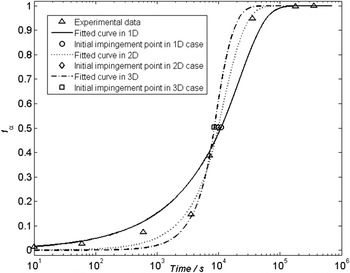
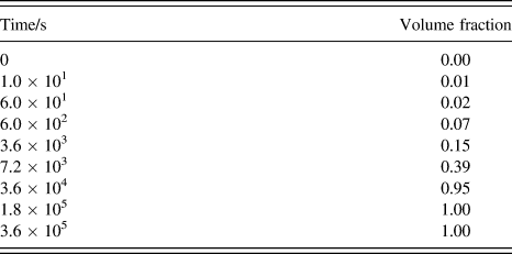
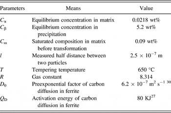
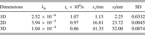
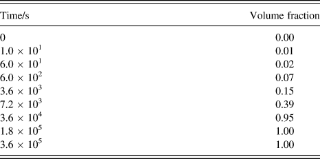
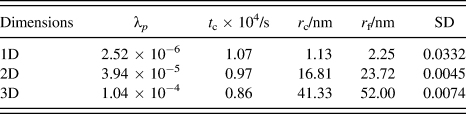
The transformed mass fraction is obtained by weighing the chemical extraction. The volume fraction of M23C6 is replaced by the mass fraction because the normalization will need to be performed.Reference Chester and Bhadeshia31 After normalization, the volume fraction (which ranges from 0 to 1) as a function of transformation time is shown in Table III. The known parameters in this model are listed in Table IV. The fitted curve in 1D, 2D, and 3D of Eq. (15) with experimental data are shown in Fig. 5, while the other calculated parameters i.e., λp, t c, r c, r f, and the standard deviation (SD) are listed in Table V. With the number of dimensions varying from 1 to 3, λp increases and t c decreases. By comparing the fitted results and the value of SD, it is indicated that the 2D model is more suitable for the precipitation of M23C6 in T92 steel, where the value of λp is 3.938 × 10⁻⁵, and t c is 9686 s. In the 2D model, M23C6 particle are assumed as a cylinder,Reference Abe, Horiuchi, Taneike and Sawada32 with r 0 being its radius and l the half distance between two adjacent particles.
Fitted curve of f-t with experimental data in case of 1D, 2D, and 3D.

Volume fraction obtained by weighing the mass fraction followed by normalization.
Known parameters in the model.

The fitted growth coefficient and the other parameters calculated from Eq. (15) in case of 1D, 2D, and 3D respectively.
A. Effect of l on the precipitation of M23C6
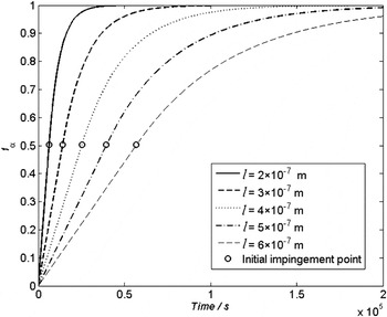
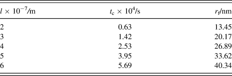
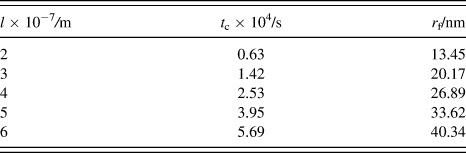
l is an important parameter in the precipitation model. A higher l value means a lower nuclei number existing in site saturation at the beginning of the isothermal transformation, according to the definition of site saturation nucleation.Reference Liu, Nitsche, Sommer and Mittemeijer7 The value of l measured from TEM images is approximately equal to the width of martensite lath. As the M23C6 carbides are nucleated along martensite laths and former austenite boundaries, the value of l varies with different initial microstructure conditions, such as different lath width or prior austenite grain size. The smaller the lath width or austenite grain size is, the smaller the value of l is. Upon Eq. (15), and fitted λ2 in the case of 2D, the transformed fraction as a function of time can be predicted with different values of l, as shown in Fig. 6, and the calculated t c and r f are listed in Table VI. A higher value of l leads to a longer transformation time, i.e., the postponing of the initial time of soft impingement and the entire transformation time. Moreover, the position of growth front at the end of transformation r f increases significantly as l increases, suggesting that the final particle size of precipitates at the end of transformation is larger due to a larger grain size or lath width, and meanwhile, the distribution density is lower according to the basis of site saturation nucleation. Therefore, fine grain size is conducive to the dispersion of M23C6 precipitates.
Predicted curve of f-t with different value of l in case of 2D.

The change of calculated parameters as a function of different l.
B. Prediction of M23C6 precipitation at different temperatures
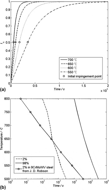
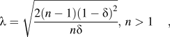
Zener had suggested that the growth coefficient λp is temperature-independent,Reference Zener21 and accordingly, the precipitation of M23C6 can be predicted using Eq. (17) with the fitted value of λp. The prediction of transformed fraction as a function of time at different temperatures is shown in Fig. 7(a). The transformation time is prolonged with decreasing of holding temperature because of the lowering of the diffusion coefficient D of carbon. Then, the time-temperature-transformation (TTT) diagram of M23C6 precipitation can be obtained from the f-t curve under different temperatures, as shown in Fig. 7(b): the onset and the end time are corresponding to the precipitation fraction 2% and 98% respectively. However, comparing with the data calculated by Robson and Bhadeshia,Reference Robson and Bhadeshia33 the slope of the predicted TTT diagram is steeper, which means that the onset time of precipitation is delayed at high temperatures and advanced at low temperatures. This phenomenon is due to the temperature-independence of growth. The classic growth coefficient of partitioning phase transformations in binary alloys is derived by solving the diffusion equationsReference Chen and van der Zwaag14:
 $${\rm{\lambda }} = \sqrt {{{2\left( {n - 1} \right)\left( {1 - {\rm{\delta }}} \right)^2 } \over {n{\rm{\delta }}}}} ,\,n > 1\,\quad,$$
Prediction of M23C6 precipitation in T92 steel: (a) The f-t curve with different temperature in case of 2D, where the growth coefficient is time-independent; (b) TTT diagram of M23C6 precipitation based on the f-t curve and the comparison with the data in Ref. Reference Robson and Bhadeshia33, where an obvious discrepancy can be found.

when n = 2, it would become linear approximation, when n = 3, the diffusion field would be quadratic. This equation suggests that the growth coefficient is dependent only on the degree of supersaturation.
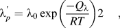
Therefore, a temperature-dependent growth coefficient  ${\rm{\lambda }}_p^\prime$ is taken into account for reducing the discrepancy. The growth coefficient at different temperatures can be described by Arrhenius equation:
 $${\rm{\lambda }}_p^\prime = {\rm{\lambda }}_0 \exp \left( {{{ - Q_{\rm{\lambda }} } \over {RT}}} \right)2\,\quad,$$
where λ0 is the preexponential factor, and Q λ is the activation energy of growth. It is obvious that  ${\rm{\lambda }}_p^\prime$ increases with the elevation of temperature by comparing Eqs. (16) and (17). The final equation with temperature-dependent growth coefficient can be obtained by substituting Eq. (17) into Eq. (15):
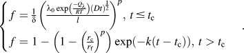 $$\!\!\!\left\{ \matrix{ f = {1 \over {\rm{\delta }}}\left( {{{{\rm{\lambda }}_0 \exp \left( {{{ - Q_{\rm{\lambda }} } \over {RT}}} \right)\left( {Dt} \right)^{{1 \over 2}} } \over l}} \right)^p ,\,t \,\le\, t_{\rm{c}} \hfill \cr f = 1 - \left( {1 - \left( {{{r_{\rm{c}} } \over {r_{\rm{f}} }}} \right)^p } \right)\exp \left( { - k\left( {t - t_{\rm{c}} } \right)} \right),\,t > t_{\rm{c}} \hfill \cr} \right.\quad\,.$$
By fitting Eq. (18) with experimental data in 2D case, the value of λ0 and Q λ can be obtained, and the calculated initial time of soft impingement t c and the SD are listed in Table VII. As the growth of M23C6 is controlled by carbon diffusion, the activation energy of M23C6 growth is nearly equal to the diffusion activation energy of carbon in martensite. Similarly, the prediction of f-t curve can be given by Eq. (18) and then the TTT diagram is obtained based on the f-t curve at different temperatures, as shown in Fig. 8. It is shown that, the onset time of precipitation advanced at elevated temperature and delayed at low temperature, by comparing with Fig. 7. With the change of growth coefficient  ${\rm{\lambda }}_p\!\!\!\prime\,$, the predicted TTT diagram is consistent with the data calculated by Ref. Reference Robson and Bhadeshia33. The results suggest that, the assumption for the temperature-dependent growth coefficient is reasonable.
Prediction of M23C6 precipitation in T92 steel with temperature-dependent  ${\rm{\lambda }}_p^\prime$: (a) The f-t curve with different temperature in case of 2D; (b) TTT diagram of M23C6 precipitation based on the f-t curve and the comparison with the data in Ref. Reference Robson and Bhadeshia33, where an agreement is achieved.

The calculated parameters with a temperature-dependent growth coefficient by fitting Eq. (17) with experimental data at 650 °C in 2D case. Notes that, Q G is approximately equal to diffusion coefficient of carbon in martensite, and  ${\rm{\lambda }}_p^\prime$ is approximately equal to λp at 650 °C.

V. CONCLUSION
The kinetics model for transformation is obtained by assuming the site saturated nucleation, diffusion controlled growth and soft-impingement, which has been found suitable for the precipitation of M23C6 during tempering in the case of 2D compared with the fitted results. As l is an essential parameter, which affects the final particle size and density distribution of precipitates significantly, fine grain size is beneficial to the dispersion of M23C6. Using a temperature-dependent growth coefficient, the prediction is more accurate at elevated and low temperatures. The growth coefficient  ${\rm{\lambda }}_p^\prime$ can be described by Arrhenius equation, and the activation energy of growth Q G is nearly equal to the activation energy of carbon diffusion, suggesting that the growth is diffusion-controlled.
ACKNOWLEDGMENTS
The authors are grateful to the National Natural Science Foundation of China, Shanghai Baosteel Group Company (Grant No. 50834011) and the National Natural Science Foundation of China (Grant Nos. 51104107 and No. 51204121) for grant and financial support.