2 Governing equations and numerical methods

The incompressible Navier–Stokes (NS) equations in primitive variables are considered

(2.1) $$\begin{eqnarray}\displaystyle \unicode[STIX]{x2202}_{t}u_{i}+u_{j}\unicode[STIX]{x2202}_{j}u_{i}=-\unicode[STIX]{x2202}_{i}p+\unicode[STIX]{x1D708}\unicode[STIX]{x2202}_{j}^{2}u_{i};\quad \unicode[STIX]{x2202}_{i}u_{i}=0, & & \displaystyle\end{eqnarray}$$

where $u_{i}$ is the velocity field, $p$ represents the kinematic pressure and $\unicode[STIX]{x1D708}$ is the kinematic viscosity. A schema of the problem under consideration is shown in figure 1.

Figure 1.

Schematic figure of the backward-facing step problem, $ER=H/(H-h)=2$ , and details about its geometry and grid spacing (size of zones and concentration factors; arrows indicate the grid refinement direction). Not to scale.

The dimensions of the computational domain are $38h\times 2h\times 2\unicode[STIX]{x03C0}h$ in the streamwise, normal and spanwise directions, respectively. The sudden expansion is located at $L_{u}=6h$ from the inflow, whereas the domain length downstream of the step is divided into two parts $(L_{d1}=1h,L_{d2}=31h)$ for refinement reasons. The origin of coordinates is placed at the expansion sharp edge. A detailed discussion about the determination of the domain size and grid spacing is given in the next section.

Regarding the boundary conditions, a turbulent channel flow is imposed at the inflow following the same strategy used by Meri & Wengle (Reference Meri, Wengle, Friedrich and Rodi2002), whereas a convective boundary condition is used at the outflow, $\unicode[STIX]{x2202}_{t}u_{i}+0.5U_{b}\unicode[STIX]{x2202}_{1}u_{i}=0$ . Global mass conservation may be not exactly preserved after imposing such boundary conditions. It is forced by means of a minor correction (a constant many orders of magnitude lower than $U_{b}$ ) at the outflow conditions. Finally, periodic boundary conditions are imposed in the spanwise direction, and no-slip boundary conditions are imposed at the walls.

The incompressible NS equations (2.1) are discretized on a non-uniform structured staggered mesh, and a fourth-order symmetry-preserving discretization (Verstappen & Veldman Reference Verstappen and Veldman2003) scheme is used. Briefly, the temporal evolution of the spatially discrete staggered velocity vector, $\boldsymbol{u}_{s}$ , is governed by the following operator-based finite-volume discretization of (2.1),

(2.2) $$\begin{eqnarray}\unicode[STIX]{x1D734}\frac{\text{d}\boldsymbol{u}_{s}}{\text{d}t}+\unicode[STIX]{x1D63E}\left(\boldsymbol{u}_{s}\right)\boldsymbol{u}_{s}+\unicode[STIX]{x1D63F}\boldsymbol{u}_{s}-\unicode[STIX]{x1D648}^{t}\boldsymbol{p}_{c}=\mathbf{0}_{s},\end{eqnarray}$$

where the subscripts $s,c$ refer to discrete staggered and collocated vectors, respectively. The discrete incompressibility constraint is given by $\unicode[STIX]{x1D648}\boldsymbol{u}_{s}=\mathbf{0}_{h}$ , where $\unicode[STIX]{x1D648}$ indicates the divergence matrix. The diffusive matrix, $\unicode[STIX]{x1D63F}$ , is symmetric and positive semi-definite, representing the integral of the diffusive flux, $-\unicode[STIX]{x1D708}\unicode[STIX]{x2202}_{j}u_{i}n_{j}$ , through the faces (where $n_{j}$ refers to a normal surface direction). The diagonal matrix, $\unicode[STIX]{x1D734}$ , describes the sizes of the control volumes and the approximate, convective flux is discretized as in Verstappen & Veldman (Reference Verstappen and Veldman2003). The resulting convective matrix, $\unicode[STIX]{x1D63E}\left(\boldsymbol{u}_{s}\right)$ , is skew–symmetric, i.e.

(2.3) $$\begin{eqnarray}\unicode[STIX]{x1D63E}\left(\boldsymbol{u}_{s}\right)=-\unicode[STIX]{x1D63E}^{t}\left(\boldsymbol{u}_{s}\right)\!.\end{eqnarray}$$

In a discrete setting, the skew–symmetry of $\unicode[STIX]{x1D63E}\left(\boldsymbol{u}_{s}\right)$ implies that

(2.4) $$\begin{eqnarray}\unicode[STIX]{x1D63E}\left(\boldsymbol{u}_{s}\right)\boldsymbol{v}_{s}\boldsymbol{\cdot }\boldsymbol{w}_{s}=\boldsymbol{v}_{s}\boldsymbol{\cdot }\unicode[STIX]{x1D63E}^{t}\left(\boldsymbol{u}_{s}\right)\boldsymbol{w}_{s}=-\boldsymbol{v}_{s}\boldsymbol{\cdot }\unicode[STIX]{x1D63E}\left(\boldsymbol{u}_{s}\right)\boldsymbol{w}_{s},\end{eqnarray}$$

for any discrete velocity vector $\boldsymbol{u}_{s}$ (if $\unicode[STIX]{x1D648}\boldsymbol{u}_{s}=\mathbf{0}_{s}$ ), $\boldsymbol{v}_{s}$ and $\boldsymbol{w}_{s}$ . The evolution of the discrete energy, $\Vert \boldsymbol{u}_{s}\Vert ^{2}=\boldsymbol{u}_{s}\boldsymbol{\cdot }\unicode[STIX]{x1D734}\boldsymbol{u}_{s}$ , is governed by

(2.5) $$\begin{eqnarray}\frac{\text{d}}{\text{d}t}\Vert \boldsymbol{u}_{s}\Vert ^{2}=-2\boldsymbol{u}_{s}\boldsymbol{\cdot }\unicode[STIX]{x1D63F}\boldsymbol{u}_{s}<0,\end{eqnarray}$$

where the convective and pressure gradient contributions cancel because of (2.3) and the incompressibility constraint, $\unicode[STIX]{x1D648}\boldsymbol{u}_{s}=\mathbf{0}_{c}$ , respectively. Therefore, even for coarse grids, the energy of the resolved scales of motion is convected in a stable manner, i.e. the discrete convective operator transports energy from a resolved scale of motion to other resolved scales without dissipating any energy, as it should be from a physical point of view. For a detailed explanation, the reader is referred to Verstappen & Veldman (Reference Verstappen and Veldman2003).

The governing equations are integrated in time using a classical fractional step projection method (Chorin Reference Chorin1968). Namely, the solution of the unsteady Navier–Stokes equations is obtained by first time advancing the velocity field, $\boldsymbol{u}_{s}^{n}$ , without regard for its solenoidality constraint, then recovering the proper solenoidal velocity field, $\boldsymbol{u}_{s}^{n+1}$ ( $\unicode[STIX]{x1D648}\boldsymbol{u}_{s}=\mathbf{0}_{c}$ ). For the temporal discretization, a second-order fully explicit one-leg scheme is used for both the convective and diffusive terms (Trias & Lehmkuhl Reference Trias and Lehmkuhl2011). Thus, the resulting fully discretized problem reads

(2.6) $$\begin{eqnarray}\displaystyle \frac{(\unicode[STIX]{x1D705}+1/2)\boldsymbol{u}_{s}^{p}-2\unicode[STIX]{x1D705}\boldsymbol{u}_{s}^{n}+(\unicode[STIX]{x1D705}-1/2)\boldsymbol{u}_{s}^{n-1}}{\unicode[STIX]{x0394}t}=\unicode[STIX]{x1D64D}((1+\unicode[STIX]{x1D705})\boldsymbol{u}_{s}^{n}-\unicode[STIX]{x1D705}\boldsymbol{u}_{s}^{n-1}), & & \displaystyle\end{eqnarray}$$

where $\unicode[STIX]{x1D64D}(\boldsymbol{u}_{s})=-\unicode[STIX]{x1D63E}\left(\boldsymbol{u}_{s}\right)\boldsymbol{u}_{s}-\unicode[STIX]{x1D63F}\boldsymbol{u}_{s}$ and $\boldsymbol{u}_{s}^{p}$ is a predictor velocity that can be directly evaluated from the previous expression. The time-integration parameter, $\unicode[STIX]{x1D705}$ , is computed to adapt the linear stability domain of the time-integration scheme to the instantaneous flow conditions in order to use the maximum time step possible. For further details about the time-integration method the reader is referred to Trias & Lehmkuhl (Reference Trias and Lehmkuhl2011). Finally, $\boldsymbol{u}_{s}^{p}$ must be projected onto a divergence-free space,

(2.7) $$\begin{eqnarray}\boldsymbol{u}_{s}^{n+1}=\boldsymbol{u}_{s}^{p}+\unicode[STIX]{x1D734}^{-1}\unicode[STIX]{x1D648}^{t}\tilde{\boldsymbol{p}}_{c}^{n+1},\end{eqnarray}$$

by adding the gradient of the pseudo-pressure, $\tilde{\boldsymbol{p}}_{c}=\unicode[STIX]{x0394}t/(\unicode[STIX]{x1D705}+1/2)\boldsymbol{p}_{c}$ , satisfying the following Poisson equation

(2.8) $$\begin{eqnarray}\unicode[STIX]{x1D647}\tilde{\boldsymbol{p}}_{c}^{n+1}=\unicode[STIX]{x1D648}\boldsymbol{u}_{s}^{p}\quad \text{with }\unicode[STIX]{x1D647}=-\unicode[STIX]{x1D648}\unicode[STIX]{x1D734}^{-1}\unicode[STIX]{x1D648}^{t},\end{eqnarray}$$

where the discrete Laplacian operator, $\unicode[STIX]{x1D647}$ , is represented by a symmetric negative semi-definite matrix. For details about the numerical algorithms and the parallel Poisson solver, the reader is referred to Gorobets, Trias & Oliva (Reference Gorobets, Trias and Oliva2013). Notice that the pressure is not considered in the prediction step (2.6). On staggered grids with prescribed velocity boundary conditions, as in this case, the incompressibility condition occurs naturally and no specific boundary condition for the discrete pressure field, $\boldsymbol{p}_{c}$ , needs to be specified, as pointed out in Kim & Moin (Reference Kim and Moin1985). Nevertheless, Neumann boundary conditions are prescribed for $\boldsymbol{p}_{c}$ . Regarding the verification of the code, the reader is referred, for example, to Trias et al. (Reference Trias, Soria, Oliva and Pérez-Segarra2007). The verification process of the DNS simulation carried out in this work is addressed in the next section.

3 Verification of the simulation

Averages over the two statistically invariant transformations (time and $x_{3}$ -direction) are carried out for all the fields. The standard notation $\langle \cdot \rangle$ is used to denote this averaging procedure.

During this section, the DNS results are verified using well-known tests in the literature. They are mainly focused on BFS, but the inflow quality is firstly discussed. As was mentioned before, the inflow data are obtained from a previous channel flow simulation at $Re_{\unicode[STIX]{x1D70F}}=395$ . The signal is preprocessed before being used by the BFS. A linear spatial interpolation is applied as a slightly coarser mesh is used in the BFS case because of computational cost reasons. The quality of the preprocessed inflow is assessed in figure 2, where the average streamwise velocity (a) and the root mean square (r.m.s.) (b) profiles at a certain cross-section $(-5h)$ over the step are presented. They show a good agreement with the benchmark case (Moser, Kim & Mansour Reference Moser, Kim and Mansour1999). A short distance from the inflow is selected $(6h-5h=h)$ to demonstrate that there is no need for a recovery region when this method is applied.

Figure 2.

Average streamwise velocity (a) and root-mean-square (b) profiles at $-5h$ over the step ( $1h$ downstream of the inflow). Moser et al. (Reference Moser, Kim and Mansour1999) results are used as benchmark data.

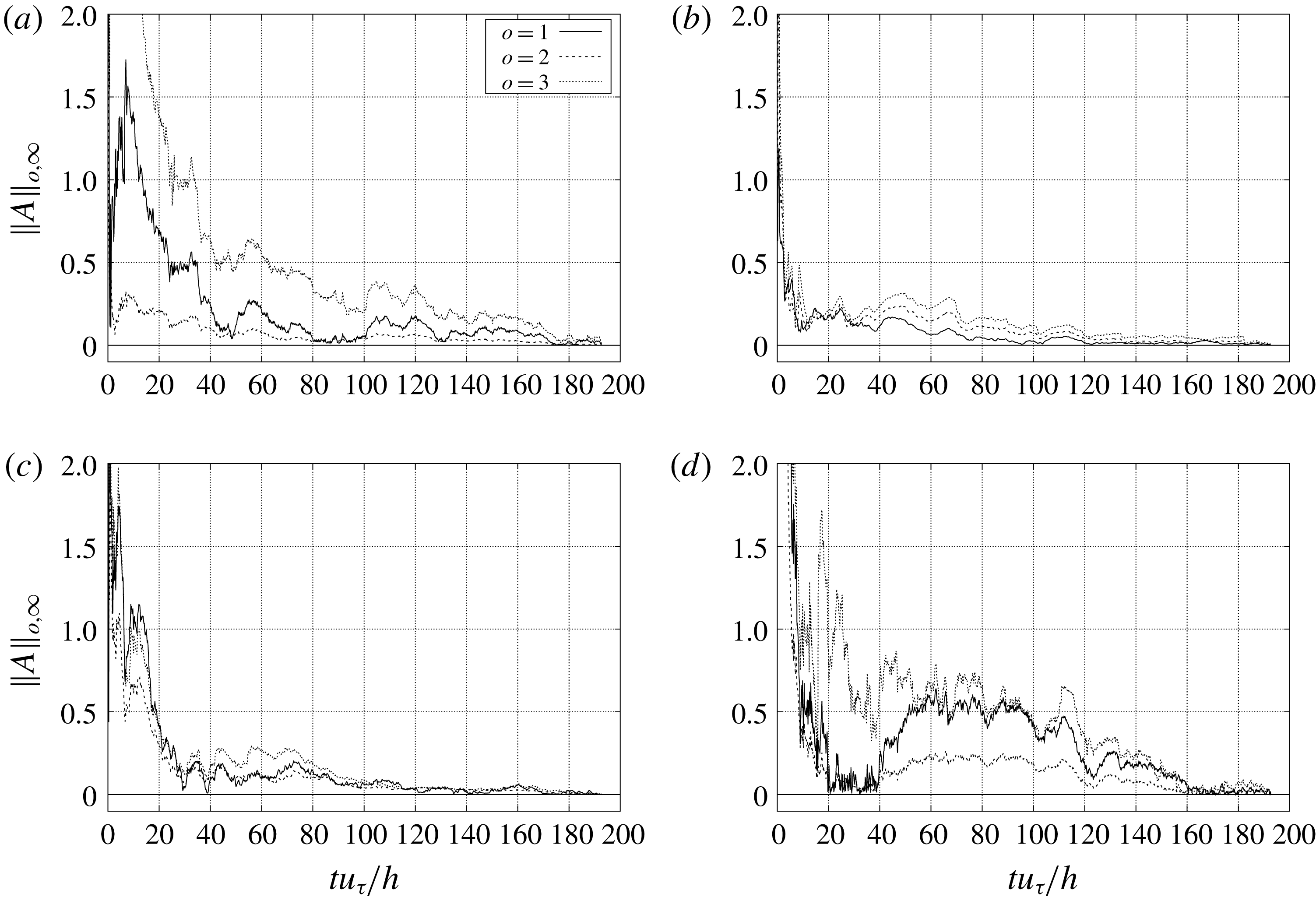
Once the behaviour of turbulence at the entrance is assessed, the minimum time integration period is determined. This has been achieved evaluating the normalized infinite norm of the first-, second- and third-order tensor turbulent statistic values at each time step (3.1).

(3.1) $$\begin{eqnarray}\Vert A\Vert _{o,\infty }(t_{s})=\max _{n}^{N}\left|1-\frac{1}{\langle a_{o,n}\rangle }\int _{0}^{t_{s}}a_{o,n}\,\text{d}t\right|,\end{eqnarray}$$

where $[a_{o}]$ denotes a list of $N$ elements, which depends on the order $(o)$ , and $n$ refers to a specific list element, $a_{o,n}$ . The symbology $[\cdot ]$ converts any tensor in a list of elements. Elements presenting average values, $\langle a_{o,n}\rangle$ , close to zero are excluded in order to avoid $0/0$ indeterminate forms. The maximum absolute value in a list of $N$ elements is selected at each $t_{s}$ , and denoted as $\Vert A\Vert _{o,\infty }(t_{s})$ . For instance, the first-order list ( $N=3$ ) is filled by all velocity components ( $[a_{1}]=[u_{i}]$ ), whereas the second-order list ( $N=9$ ) includes all second-order tensor elements ( $[a_{2}]=[u_{i}u_{j}]$ ). The same explanation is valid for the third-order list. A set of probes has been distributed along the domain, but only the most important ones are shown in figures 1 and 3. The largest integration period is required at P04, where large structures dragged from the recirculation region are present. Similar behaviour is observed in the shear layer region, P01, where high velocity fluctuations also appear. The rest of the probes are located between the two recirculation bubbles, P02, and in the reattachment region, P03. A schematic view of the probes location can be observed in figure 1. In contrast to the 280 average integration time units $(h/u_{\unicode[STIX]{x1D70F}})$ suggested by Barri et al. (Reference Barri, El Khoury, Andersson and Pettersen2010), figure 3 shows that $180h/u_{\unicode[STIX]{x1D70F}}$ provides satisfactory results. This simulation time reduction can be attributed to the fact that different time integration techniques are applied. A set of individual quasi-independent flow fields separated by $0.25h/u_{\unicode[STIX]{x1D70F}}$ were taken into account by Barri et al. (Reference Barri, El Khoury, Andersson and Pettersen2010), whereas a continuous integration with time is used in the present paper. Apart from that, other factors, such as the $Re_{\unicode[STIX]{x1D70F}}$ , could also affect the integration time period. From here on, all time-average results presented in this paper have been obtained using $180h/u_{\unicode[STIX]{x1D70F}}$ , around 55 flow units ( $t_{f}=(L_{u}+L_{d}ER)/U_{b}$ ).

Figure 3.

Normalized infinite norm $(\Vert A\Vert _{o,\infty })$ (defined in (3.1)) of the first, second and third order of the non-zero velocity turbulent statistic at P01 (a), P02 (b), P03 (c) and P04 (d). Probe locations are defined in figure 1.

The BFS geometry in the spanwise and streamwise directions is also studied because of its influence in the fluid behaviour. The capability of the spanwise length to reproduce the larger scales is assessed through two-point correlations, $B_{i}^{norm}(x_{3}=0,\hat{x}_{3})=B_{i}^{norm}(\hat{x}_{3})$ , at the locations shown in figure 1:

(3.2) $$\begin{eqnarray}B_{i}^{norm}(x_{j},\hat{x}_{j})=\frac{\langle u_{i}^{\prime }(x_{j})u_{i}^{\prime }(x_{j}+\hat{x}_{j})\rangle }{\langle u_{i}^{\prime }(x_{j})\rangle \langle u_{i}^{\prime }(x_{j}+\hat{x}_{j})\rangle }.\end{eqnarray}$$

All velocity components present correlations no longer than the periodic half-length (see figure 4). Thus, the periodic direction requirement is satisfied. The largest structures appear in the recirculation bubble (P02), where the fluid becomes quasi-laminar, and the recovery region (P04). Furthermore, the streamwise length is also examined as some experimental works, such as Nadge & Govardhan (Reference Nadge and Govardhan2014), reported a systematic increase of the $X_{r}$ and the recovery region under the step when the $Re$ was increased. In particular, Nadge demonstrated that this trend exists up to $Re_{b}\approx 16300$ . Beyond this threshold, the $X_{r}$ only depends on the $ER$ . In the present paper, and despite the recirculation length increase with respect to the case studied by Barri et al. (Reference Barri, El Khoury, Andersson and Pettersen2010), the recirculation zone remains far enough to be affected by the outflow effects. More information regarding the streamwise length can be obtained in § 4.

Figure 4.

Two-point correlation in the spanwise direction of three velocity components at P01, P02, P03 and P04 locations (see figure 1). The integral scale value ( $L$ ) of each cross-correlation is presented at the legend. Streamwise (a), normal (b) and spanwise (c) components.

Once the physical parameters are controlled, the grid resolution and the time step need to be determined. A Cartesian staggered mesh with $1510\times 302\times 360$ grid points has been used to cover the computational domain. The grid spacing in the periodic $x_{3}$ -direction is uniform, whereas the rest of the directions use piecewise hyperbolic–tangent functions. For example, the distribution of points in the $x_{2}$ -direction corresponding to the step region, i.e. $-h\leqslant x_{2}\leqslant 0$ , is given by

(3.3) $$\begin{eqnarray}x_{2,k}=x_{2,0}^{a}+\frac{h}{2}\left(1+\frac{\tanh \{\unicode[STIX]{x1D6FE}_{2}^{a}(2(k-1)/N_{2}-1)\}}{\tanh \unicode[STIX]{x1D6FE}_{2}^{a}}\right),\quad k=1,\ldots ,N_{2}+1,\end{eqnarray}$$

where the starting point, the number of grid points and the refinement factor are $x_{2,0}^{a}=-h$ , $N_{2}=302/2$ and $\unicode[STIX]{x1D6FE}_{2}^{a}=1.16855$ . The same is true above the step region, but using $x_{2,0}^{a}=0$ . In these regions, the mesh is refined in both directions. The grid refinement formula needs to be properly adapted for those areas where the mesh is refined only in one direction (see figure 1 for details). For example, the grid points in the region upstream of the step, i.e. $-L_{u}\leqslant x_{1}\leqslant 0$ , are distributed as follows

(3.4) $$\begin{eqnarray}x_{1,k}=x_{1,0}^{l}+\frac{L_{1}^{l}}{2}\left(1+\frac{\tanh \{\unicode[STIX]{x1D6FE}_{1}^{l}((k-1)/N_{1}^{l}-1)\}}{\tanh \unicode[STIX]{x1D6FE}_{1}^{l}}\right),\quad k=1,\ldots ,N_{1}^{l}+1,\end{eqnarray}$$

where $l$ refers to the zone which is being studied ( $a$ , $b$ , $c$ ). In this case $l=a$ , while the starting point, the region length and the refinement factor are $x_{1,0}^{a}=-L_{u}$ , $L_{1}^{a}=L_{u}$ and $\unicode[STIX]{x1D6FE}_{1}^{a}=1.1$ , respectively. The same technique is applied in the outflow region ( $l=c$ ), where $x_{1,0}^{c}=L_{d1}$ and $\unicode[STIX]{x1D6FE}_{1}^{c}=1.5$ . There are no arrows in region $l=b$ , as a uniform distribution is imposed in order to increase the mesh resolution in this area and to capture the shear layer phenomena. Finally, the number of grid points follows straightforwardly by imposing that $N_{1}^{a}+N_{1}^{b}+N_{1}^{c}=N_{1}=1510$ , and that the sizes of two consecutive control volumes corresponding to different areas are equal. The grid points in the $x_{2}$ -direction are distributed following the same restrictions.

Figure 5.

Mesh dimensions next to the upper ( $UW$ ) and lower ( $LW$ ) walls expressed in wall units ( $\unicode[STIX]{x1D6FF}_{+}=\unicode[STIX]{x1D708}/u_{\unicode[STIX]{x1D70F}}$ ).

Mesh quality has been assessed using the present DNS results, analysing the control volume size next to the wall and at the core. The former is evaluated using wall units, whereas a comparison with the estimated Kolmogorov length scales is performed with the latter. Figure 5 presents the mesh dimensions in wall units at the upper and lower walls along the streamwise direction. It can be noticed that the mesh refinement at the lower wall upstream of the step ( $x_{1}\leqslant 0$ ) has not been provided as it exhibits a similar behaviour to the upper wall (difference less than 1.5 %). Hence, figure 5 shows how the selected mesh is fine enough in all directions to perform a channel flow DNS upstream and downstream of the step edge. In particular, the mesh dimension in the normal direction is $\unicode[STIX]{x0394}x_{2}^{+}\lesssim 1.3$ . A mesh decrease in wall units is observed in all directions just under the step (lower wall) due to the fact that the recirculation bubbles smooth the velocity gradients close to the wall. Although this decrease also affects $\unicode[STIX]{x0394}x_{1}^{+}$ , its reduction is mainly caused by the mesh refinement in order to capture the well-known massive expansion phenomenon. It is worth noting here that both walls lead to the same channel flow behaviour far away from the step edge (recovery region).

Regarding the mesh quality at the core of the BFS, the ratio of different spatial length scales versus the estimated Kolmogorov length scale, $\unicode[STIX]{x1D702}=(\unicode[STIX]{x1D708}^{3}/\langle \unicode[STIX]{x1D700}\rangle )^{1/4}$ , have been evaluated in the sudden expansion zone. Where $\langle \unicode[STIX]{x1D700}\rangle$ refers to the turbulent kinetic energy dissipation term. The spatial length scale would define the smallest scales that can be created in a given mesh, which not only depends on the mesh itself but also on the flow behaviour. In this context, two common approaches for assessing the spatial length scales are considered: the ratio of the maximum local control volume dimension, $\unicode[STIX]{x1D6E5}_{max}=\max (\unicode[STIX]{x0394}x_{1},\unicode[STIX]{x0394}x_{2},\unicode[STIX]{x0394}x_{3})$ , and the cube root of the cell volume, $\unicode[STIX]{x1D6E5}_{\forall }=(\unicode[STIX]{x0394}x_{1}\unicode[STIX]{x0394}x_{2}\unicode[STIX]{x0394}x_{3})^{1/3}$ . The former is preferable in zones with isotropic-like turbulence, while the latter performs better in zones where important anisotropies are present (Shur et al. Reference Shur, Spalart, Strelets and Travin2015). The effects of the spatial length scale in the sudden expansion zone can be observed in figure 6, where the ratio values using both scales are displayed. First, the highest values in both (a) and (b) are located downstream of the step edge and at the reattachment zone. The former is caused by the shear layer effects, while the latter is attributed to the mesh coarsening in the streamwise direction. In addition, the ratio $\unicode[STIX]{x1D6E5}_{max}/\unicode[STIX]{x1D702}$ (a) generally presents higher values than $\unicode[STIX]{x1D6E5}_{\forall }/\unicode[STIX]{x1D702}$ (b).

It is worth noting here that, even though $\unicode[STIX]{x1D6E5}_{max}/\unicode[STIX]{x1D702}$ (a) is considerably larger at the shear layer, it is not a suitable criterion due to the high flow anisotropies (two-dimensional-like). Therefore, in this case the $\unicode[STIX]{x1D6E5}_{\forall }$ (b) ratio would be more representative. The contrary is true downstream of the shear layer, at the core of the channel, where the flow starts the recovery process. In any case, values higher than 10 are not observed, which is similar to the resolution requirements discussed by Trias, Gorobets & Oliva (Reference Trias, Gorobets and Oliva2015). In this regard, a recent work carried out by Vreman & Kuerten (Reference Vreman and Kuerten2014) has shown that most of the dissipation in a turbulent channel flow occurs at scales greater than $30\unicode[STIX]{x1D702}$ . Finally, a good agreement with the results provided by Meri & Wengle (Reference Meri, Wengle, Friedrich and Rodi2002) has also been observed, although these authors provided only shorthand information regarding this verification part.

Figure 6.

Mesh quality assessment, comparing different local spatial scales with the Kolmogorov length scale, $\unicode[STIX]{x1D702}$ . Those are: the maximum local control volume dimension (a), $\unicode[STIX]{x1D6E5}_{max}$ , and the cell volume cube root (b), $\unicode[STIX]{x1D6E5}_{\forall }$ .

4 Results and discussion

The average flow fields and the time-dependent signals collected during the simulation are discussed in this section. For the sake of clarity, this work only contains the most significant results according to the authors’ criterion. All data obtained in this research are publicly available on the internet (Pont-Vílchez et al. Reference Pont-Vílchez, Trias, Gorobets and Oliva2018).

4.1 Time-averaged flow

The pressure coefficient distribution, $\langle C_{p}\rangle =(\langle p\rangle -p_{o})/(1/2)U_{c}^{2}$ , the velocity components and the streamlines of the average flow in the recirculation region are shown in figure 7. Here, $p_{o}$ refers to the kinematic pressure at the step edge. The sudden expansion leads to a massive flow separation (c), and its respective adverse pressure gradient (a). The velocity field distribution (b) is consistent with the pressure rise and the streamlines. Velocity components are depicted in a different manner in order to improve visualization and provide a dynamic perception. The $\langle C_{p}\rangle$ rise at the lower wall across the streamwise direction is detailed in figure 8(b). DNS data show a good agreement in comparison to the experimental work carried out by Ötügen (Reference Ötügen1991), although higher adverse pressure gradients were detected by this author. The skin friction, $\langle C_{f}\rangle =\langle \unicode[STIX]{x1D70F}_{w}\rangle /(1/2)\unicode[STIX]{x1D70C}U_{c}^{2}$ , is also presented in the same figure at the upper and lower walls (a), and compared to the numerical DNS results obtained by Barri et al. (Reference Barri, El Khoury, Andersson and Pettersen2010) ( $Re_{\unicode[STIX]{x1D70F}}=180,ER=2$ ). Regarding the Jovic & Driver (Reference Jovic and Driver1995) study, a significant reduction of the $\langle C_{f}\rangle$ negative peak located at the lower wall ( $LW$ ) is perceived when the $Re_{b}$ increases. This points out a depletion of the diffused momentum in the recirculation region with respect to the amount of momentum that is entering through the inflow. According to the literature, the $X_{r}$ elongation phenomenon is also observed, exhibiting an $X_{r}$ equal to $8.8h$ at $Re_{\unicode[STIX]{x1D70F}}=395$ and $7.1h$ at $Re_{\unicode[STIX]{x1D70F}}=180$ . This trend is detailed in figure 9, where the DNS results of different authors are compared with the experimental results obtained by Nadge & Govardhan (Reference Nadge and Govardhan2014). The present DNS is not only close to the asymptotic region, but also exhibits a good agreement with the experimental data (relative difference ${\leqslant}3.5\,\%$ ). It is worth noting that the $X_{r}$ value reported by Ötügen (Reference Ötügen1991) is not presented in this figure as the author evaluated this coefficient considering other methodologies. Even so, not all results provided by Ötügen (Reference Ötügen1991) have been disregarded, such as the streamwise velocity and r.m.s. profiles, which have been compared with the present DNS at different locations in figure 10. Although some differences can be observed, an acceptable agreement is present in both variables. The discrepancies observed between the experimental and numerical data could be related to the important scattering registered by Nadge & Govardhan (Reference Nadge and Govardhan2014). The author reflected his concerns about this topic, concluding that other elements in addition to the Reynolds number and the $ER$ could affect the massive expansion behaviour. In particular, the flow performance just before the sudden expansion is considered an influential factor, although it has not been commonly reported in the literature. In this paper a $Re_{\unicode[STIX]{x1D70F}}=400.5$ and a turbulence intensity in the streamwise direction equal to $u_{rms}/U_{c}\approx 3.8\,\%$ are observed. Hence, the lack of agreement observed in figure 10 could be attributed to the fluid behaviour misalignments at the step edge.

Figure 7.

(a) Pressure coefficient distribution, $\langle C_{p}\rangle$ , (b) the average velocity field, $\langle u_{i}\rangle$ , and (c) flow streamlines in the recirculation region. For the sake of clarity, the streamwise velocity, $\langle u_{1}\rangle$ , is indicated using solid lines, whereas the normal velocity component, $\langle u_{2}\rangle$ , is depicted using isolines (where dashed lines denote positive values and dot-dashed lines denote negative ones). The $\langle u_{1}\rangle$ values have been normalized using the maximum velocity of each profile, following the Ötügen (Reference Ötügen1991) criterion.

Figure 8.

Comparison of the skin friction (a), $\langle C_{f}\rangle$ , at $Re_{\unicode[STIX]{x1D70F}}=395$ (present DNS) with the results obtained by Barri et al. (Reference Barri, El Khoury, Andersson and Pettersen2010) at $Re_{\unicode[STIX]{x1D70F}}=180$ using an $ER=2$ . The $\langle C_{f}\rangle$ is assessed at the lower $(LW)$ and upper $(UW)$ walls. Pressure coefficient (b), $\langle C_{p}\rangle$ , at the $LW$ obtained in the present DNS compared to the results provided by Barri et al. (Reference Barri, El Khoury, Andersson and Pettersen2010),  $Re_{\unicode[STIX]{x1D70F}}=180$ , and Ötügen (Reference Ötügen1991),  $Re_{\unicode[STIX]{x1D70F}}=395$ .

Figure 9.

Recirculation length ( $X_{r}$ ) using different Reynolds numbers ( $Re_{b}$ ) and expansion ratios ( $ER$ ). Experimental results depicted by lines were obtained by Nadge & Govardhan (Reference Nadge and Govardhan2014).

Figure 10.

Streamwise velocity (a) and r.m.s. (b) profiles of the present DNS (——) compared to the experimental results ( $\odot$ ) obtained by Ötügen (Reference Ötügen1991). Velocity ( $u_{1}$ ) and r.m.s. values are normalized using the maximum value at each profile, $U_{c}$ .

The strong turbulence behaviour presented in this BFS configuration is quantified through the Reynolds stresses, as well as the production and dissipation terms derived from their respective transport equations.

(4.1) $$\begin{eqnarray}\underbrace{\unicode[STIX]{x2202}_{t}\langle u_{i}^{\prime }u_{j}^{\prime }\rangle }_{\simeq 0}+\underbrace{\langle u_{k}\rangle \unicode[STIX]{x2202}_{k}\langle u_{i}^{\prime }u_{j}^{\prime }\rangle }_{Convection}=\underbrace{\langle P_{ij}\rangle }_{Production}+\underbrace{\langle \unicode[STIX]{x1D6F1}_{ij}\rangle }_{Pressure-Strain}+\underbrace{\langle D_{ij}\rangle }_{Diffusion~Terms}-\underbrace{\langle \unicode[STIX]{x1D700}_{ij}\rangle }_{Dissipation},\end{eqnarray}$$

where:

(4.2a ) $$\begin{eqnarray}\displaystyle \langle P_{ij}\rangle & = & \displaystyle -\langle u_{i}^{\prime }u_{k}^{\prime }\rangle \unicode[STIX]{x2202}_{k}\langle u_{j}\rangle -\langle u_{j}^{\prime }u_{k}^{\prime }\rangle \unicode[STIX]{x2202}_{k}\langle u_{i}\rangle ,\end{eqnarray}$$

(4.2b ) $$\begin{eqnarray}\displaystyle \langle \unicode[STIX]{x1D6F1}_{ij}\rangle & = & \displaystyle \langle p^{\prime }(\unicode[STIX]{x2202}_{j}u_{i}^{\prime }+\unicode[STIX]{x2202}_{i}u_{j}^{\prime })\rangle ,\end{eqnarray}$$

(4.2c ) $$\begin{eqnarray}\displaystyle \langle D_{ij}\rangle & = & \displaystyle -\unicode[STIX]{x2202}_{k}[\langle u_{i}^{\prime }u_{j}^{\prime }u_{k}^{\prime }\rangle +(\langle p^{\prime }u_{j}^{\prime }\rangle \unicode[STIX]{x1D6FF}_{ik}+\langle p^{\prime }u_{i}^{\prime }\rangle \unicode[STIX]{x1D6FF}_{jk})-\unicode[STIX]{x1D708}\unicode[STIX]{x2202}_{k}\langle u_{i}^{\prime }u_{j}^{\prime }\rangle ],\end{eqnarray}$$

(4.2d ) $$\begin{eqnarray}\displaystyle \langle \unicode[STIX]{x1D700}_{ij}\rangle & = & \displaystyle 2\unicode[STIX]{x1D708}\langle \unicode[STIX]{x2202}_{k}u_{i}^{\prime }\unicode[STIX]{x2202}_{k}u_{j}^{\prime }\rangle .\end{eqnarray}$$

In order to simplify the analysis process, only the non-zero components are depicted and nearly the same layout as used by Barri et al. (Reference Barri, El Khoury, Andersson and Pettersen2010) is considered. A general increase of the Reynolds stresses is well observed in all directions in comparison to the Barri et al. (Reference Barri, El Khoury, Andersson and Pettersen2010) results. A downstream shifting of the Reynolds stress zero-gradient area can also be appreciated.

Figure 11.

Reynolds stresses $\langle u_{1}^{\prime }u_{1}^{\prime }\rangle /u_{\unicode[STIX]{x1D70F}}^{2}$ (a) and their associated transport source–sink terms scaled using $u_{\unicode[STIX]{x1D70F}}^{3}/h$ : production $\langle P_{11}\rangle$ (b), pressure–strain $\langle \unicode[STIX]{x1D6F1}_{11}\rangle$ (c) and dissipation $\langle \unicode[STIX]{x1D700}_{11}\rangle$ (d). Dashed lines depict negative values.

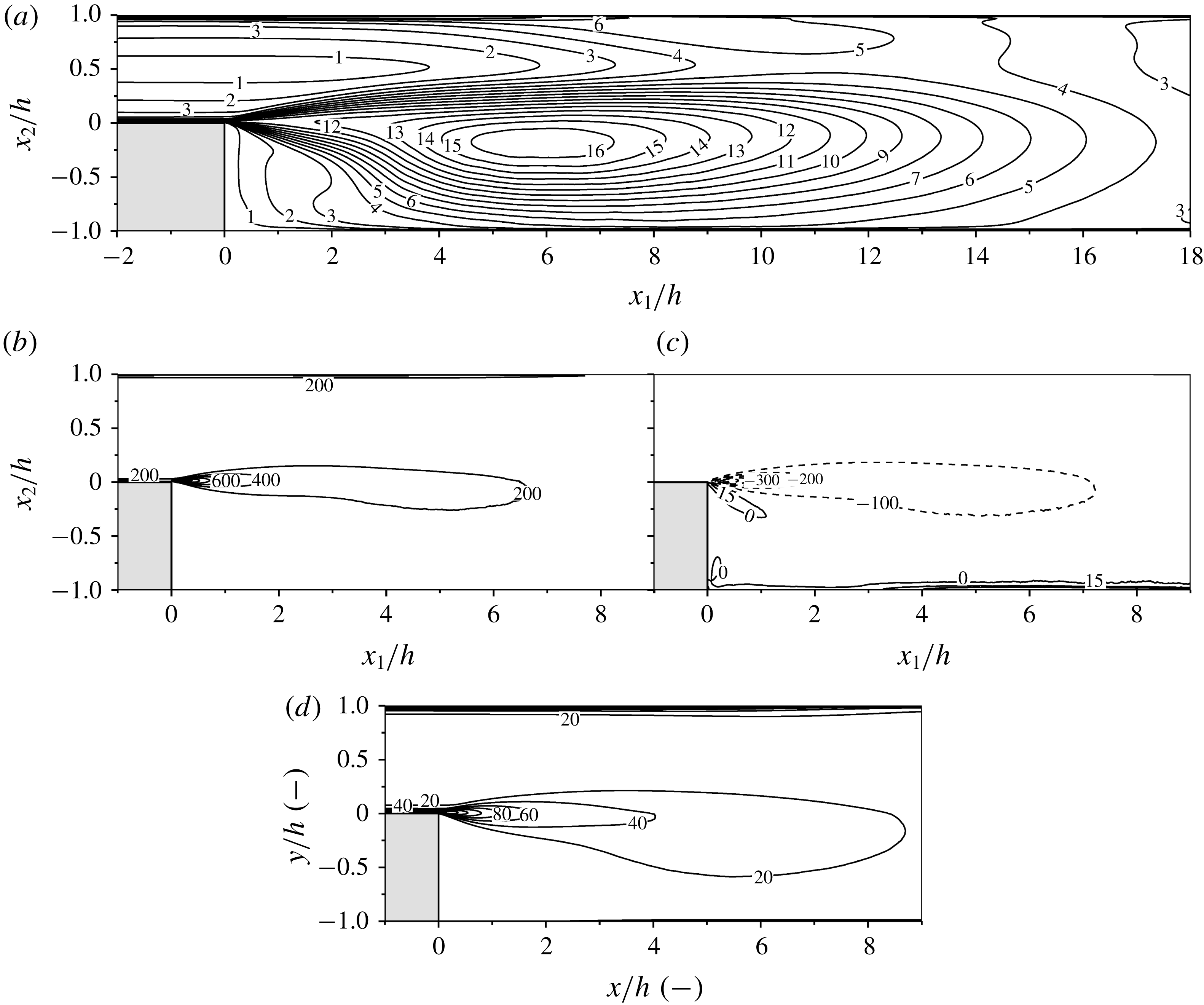
The highest momentum oscillations are in the streamwise direction, $\langle u_{1}^{\prime }u_{1}^{\prime }\rangle$ , as can be noticed in figure 11(a). This turbulence, which is triggered by the huge source term (b), is balanced by the isotropization behaviour of the pressure–strain (c). In fact, the energy from the most energetic component (streamwise) is distributed to the weakest ones (normal and spanwise directions) because of the pressure–strain phenomenon. In contrast to the channel flow behaviour, some positive values appear in the impinging regions. They are located at the end of the recirculation length and at the lower part of the shear layer. In both cases, the velocity in the streamwise direction is accelerated $\unicode[STIX]{x2202}_{1}u_{1}$ , whereas a pressure positive peak arises from the impinging interactions. As was expected, the dissipation term, $\langle \unicode[STIX]{x1D700}_{11}\rangle$ , is positive and achieves its maximum values in the shear layer and close to the walls. At the lower wall, the opposite is true due to the oscillations and gradient reduction at the recirculation bubble zone.

Figure 12.

Reynolds stresses $\langle u_{2}^{\prime }u_{2}^{\prime }\rangle /u_{\unicode[STIX]{x1D70F}}^{2}$ (a) and their associated transport source–sink terms scaled using $u_{\unicode[STIX]{x1D70F}}^{3}/h$ : production $\langle P_{22}\rangle$ (b), pressure–strain $\langle \unicode[STIX]{x1D6F1}_{22}\rangle$ (c) and dissipation $\langle \unicode[STIX]{x1D700}_{22}\rangle$ (d). Dashed lines depict negative values.

Fluctuations in the normal direction, $\langle u_{2}^{\prime }u_{2}^{\prime }\rangle$ , are shown in figure 12(a). Although in this case they are less energetic in comparison to $\langle u_{1}^{\prime }u_{1}^{\prime }\rangle$ , they remain significant. The production term (b) is non-zero, in contrast to a channel flow, and significantly lower than the pressure–strain (c). The dissipation term (d) is also positive and, as was expected, stronger in the shear layer and close to the walls.

Figure 13.

Reynolds stresses $\langle u_{3}^{\prime }u_{3}^{\prime }\rangle /u_{\unicode[STIX]{x1D70F}}^{2}$ (a) and their associated transport source–sink terms scaled using $u_{\unicode[STIX]{x1D70F}}^{3}/h$ : pressure–strain $\langle \unicode[STIX]{x1D6F1}_{33}\rangle$ (b) and dissipation $\langle \unicode[STIX]{x1D700}_{33}\rangle$ (c). Dashed lines depict negative values.

The periodic nature of the spanwise direction, $\langle u_{3}^{\prime }u_{3}^{\prime }\rangle$ , leads to an absence of the production term. However, the oscillations in this direction (see figure 13 a) are nearly as vivid as the streamwise ones. This phenomenon occurs because of the isotropization effect of the pressure–strain tensor, which converts the $\langle u_{1}^{\prime }u_{1}^{\prime }\rangle$ fluctuations into $\langle u_{3}^{\prime }u_{3}^{\prime }\rangle$ ones. The dissipation (c) term presents the same trend the above-mentioned Reynolds stresses.

Figure 14.

Reynolds stresses $-\langle u_{1}^{\prime }u_{2}^{\prime }\rangle /u_{\unicode[STIX]{x1D70F}}^{2}$ (a) and their associated transport source–sink terms scaled using $u_{\unicode[STIX]{x1D70F}}^{3}/h$ : production $\langle P_{12}\rangle$ (b), pressure–strain $\langle \unicode[STIX]{x1D6F1}_{12}\rangle$ (c) and dissipation $\langle \unicode[STIX]{x1D700}_{12}\rangle$ (d). Dashed lines depict negative values.

In order to complete the Reynolds stress assessment, the Reynolds stress non-zero cross-term ( $-\langle u_{1}^{\prime }u_{2}^{\prime }\rangle$ ) is depicted in figure 14(a). The classic axisymmetry presented in a channel flow is lost downstream of the step, but slowly recovered after the reattachment. Although this term does exhibit rather weak values (a) in comparison to the other stresses, the production (b) and pressure–strain (c) terms are quite energetic. Both terms almost present a complementary behaviour in the shear layer, explaining why the dissipation term in this zone is nearly zero.

4.2 Flow dynamics

Once the average time properties have been analysed, the time-dependent variables are assessed. An idea of the flow dynamics is given in figure 15, where the pressure gradient magnitude in the recirculation zone is shown. First, $KH$ structures are visualized just after the sharp edge (b), leading to the highest Reynolds stress values in the BFS domain (see figures 11–14). In contrast, a particular lack of pressure gradient is observed in the secondary recirculation bubble region due to its non-turbulent behaviour. Additional information is provided in the film (Pont-Vílchez et al. Reference Pont-Vílchez, Trias, Gorobets and Oliva2018), i.e. the slow motion of the recirculation bubble flow and the progressive expansion of the mainstream flow downstream of the step. The sudden expansion effects on the flow topology can also be noticed in the normal view at $x_{2}^{+}=1$ in figure 16. For instance, the turbulence triggering produced by the step edge are visualized with the $Q$ -invariant (a), showing how the highest intensity is located just downstream of the expansion. Furthermore, the channel flow streaks are also well observed in figure 16(b,c) until the sudden expansion. Downstream of the step edge, nearly ‘two-dimensional’ coherent structures are shown from 0 up to ${\sim}0.5h$ in $u_{2}^{\prime }$ (b). Beyond this threshold, the ‘two-dimensional’ coherence is lost, but the structures still grow. A similar behaviour can be observed in $u_{1}^{\prime }$ (c).

Figure 15.

Instantaneous magnitude of the dimensionless pressure gradient in a large part of the BFS domain (a), and a detailed view ( $A$ ) of the sudden expansion (b). The intensity of the fluctuation is denoted by the grey scale bar. See the film attached in the paper data base (Pont-Vílchez et al. Reference Pont-Vílchez, Trias, Gorobets and Oliva2018).

Figure 16.

A slice parallel to the lower wall at $x_{2}^{+}=1$ showing instantaneous views of the $Q$ -invariant (a), $u_{2}^{\prime }$ (b) and $u_{1}^{\prime }$ (c). Black zones denote the highest values of the $Q$ -invariant at the top figure and positive values at the bottom ones.

Besides the turbulence triggered at the step edge and its respective spreading, figures 15 and 16 also display a significant flow heterogeneity. In order to assess such diversity of flow regimes, the turbulent kinetic energy cascade at different locations has been considered (see figure 17). A schematic view of the probe locations can be observed in figure 1. Unfortunately, $KH$ instabilities are not well captured in figure 17(a), as their low energy structure effects can be easily hidden by turbulent scales coming from the channel flow boundary layer. Even so, a good trend is observed in the inertial zone ( $\bar{f}^{-5/3}$ ). It is worth noting here that the P02 frequency cascade has not been included in this figure, as the probe is located in a quasi-laminar region. Regarding the rest of $\bar{f}^{kmg}$ shown in figure 17, they diminish in the downstream direction because of the sudden expansion (P03, P04). Due to the fact that the spatial scale is $ER$ times higher at the outflow, the flow moves $ER$ times slower in order to ensure the mass conservation. Consequently, the time scale is decreased by a factor of $ER^{2}$ , bringing out the $\bar{f}^{kmg}$ trend observed (these relations can be easily demonstrated through dimensional analysis).

Figure 17.

Normalized turbulent kinetic energy ( $E_{1}$ ) versus normalized temporal frequency $(\bar{f}=fh/U_{b})$ at P01 (a), P03 (b) and P04 (c). The dashed lines represent the expected turbulence decay behaviour at the inertial region ( $\bar{f}^{-5/3}$ ), whereas $\bar{f}_{\text{P}0N}^{kmg}$ denotes the local Kolmogorov temporal frequency at probe $N$ .

Even though the ejection frequency of the $KH$ instabilities has not been well captured in P01, other interesting shear layer properties have been discerned, such as the $KH$ rates of growth along the streamwise direction. A schematic view of a shear layer is presented in figure 18, showing different structures’ size in the streamwise ( $\unicode[STIX]{x0394}\unicode[STIX]{x1D6FF}_{1}$ ) and normal ( $\unicode[STIX]{x0394}\unicode[STIX]{x1D6FF}_{2}$ ) directions.

Figure 18.

Schematic view of the Kelvin–Helmholtz vortices in a shear layer, where $\unicode[STIX]{x0394}\unicode[STIX]{x1D6FF}_{1}$ and $\unicode[STIX]{x0394}\unicode[STIX]{x1D6FF}_{2}$ represent a estimation of the vortex size in the streamwise and normal directions, respectively.

This vortex elongation was mainly attributed to the advection velocity and the vortex pairing phenomenon, which was studied by Winant & Browand (Reference Winant and Browand1974). In particular, an elliptic-like shape was experimentally detected, observing a major-to-minor axis ratio of $\unicode[STIX]{x0394}\unicode[STIX]{x1D6FF}_{1}/\unicode[STIX]{x0394}\unicode[STIX]{x1D6FF}_{2}\sim 2$ . This behaviour has been analysed with the present DNS data through the two-point correlation technique in the streamwise and normal directions. In the $\unicode[STIX]{x0394}\unicode[STIX]{x1D6FF}_{1}$ case, the distance from peak to peak (upstream) has been used to represent the distance between vortices (figure 19 a) and also to form an estimation of the average vortex size in a given position, $B_{2}^{norm}(x_{1},\hat{x}_{1})$ . In contrast, $\unicode[STIX]{x0394}\unicode[STIX]{x1D6FF}_{2}$ has been measured as the distance between zero values of the two-point correlation values, $B_{1}^{norm}(x_{2}=0,\hat{x}_{2})$ . In addition, $\unicode[STIX]{x0394}\unicode[STIX]{x1D6FF}_{2}$ has also been assessed following the equation given in Winant & Browand (Reference Winant and Browand1974),

(4.3) $$\begin{eqnarray}\unicode[STIX]{x0394}\unicode[STIX]{x1D6FF}_{2}=\unicode[STIX]{x0394}U_{1}/(\unicode[STIX]{x2202}\langle u_{1}\rangle /\unicode[STIX]{x2202}x_{2})_{max},\end{eqnarray}$$

where $\unicode[STIX]{x0394}U_{1}$ refers to the flow velocity difference in the shear layer.

Figure 19.

An example showing how $\unicode[STIX]{x0394}\unicode[STIX]{x1D6FF}_{1}$ have been assessed using the two-point correlation at the shear layer (a). Estimation of the $KH$ rate of growth ( $\unicode[STIX]{x0394}\unicode[STIX]{x1D6FF}_{1}$ , $\unicode[STIX]{x0394}\unicode[STIX]{x1D6FF}_{2}$ ) along the streamwise direction (b), which is schematically depicted in figure 18.

Two linear distributions for $\unicode[STIX]{x0394}\unicode[STIX]{x1D6FF}_{1}$ and $\unicode[STIX]{x0394}\unicode[STIX]{x1D6FF}_{2}$ have been obtained through the two-point correlation technique, showing circular structures ( $\unicode[STIX]{x0394}\unicode[STIX]{x1D6FF}_{1}\sim \unicode[STIX]{x0394}\unicode[STIX]{x1D6FF}_{2}$ ) just downstream of the step edge ( ${\sim}0.4h$ ). This is in good agreement with the ‘two-dimensional’ coherent structures observed in figure 16. Above this threshold, the circular structures are distorted, acquiring an elliptic shape ( $\unicode[STIX]{x0394}\unicode[STIX]{x1D6FF}_{1}>\unicode[STIX]{x0394}\unicode[STIX]{x1D6FF}_{2}$ ), which can be attributed to the above mentioned phenomena. This elliptical shape trend seems to be maintained along the studied domain, showing a major-to-minor axis ratio limit close to 2 ( $\unicode[STIX]{x0394}\unicode[STIX]{x1D6FF}_{1}/\unicode[STIX]{x0394}\unicode[STIX]{x1D6FF}_{2}$ ), strengthening the experimental visualizations carried out by Winant & Browand (Reference Winant and Browand1974) and supporting their theory regarding the vortex pairing (Pont-Vílchez et al. Reference Pont-Vílchez, Trias, Gorobets and Oliva2018). It is worth noting that Kostas et al. (Reference Kostas, Soria and Chong2002) observed a similar phenomenon in their BFS experimental study. Finally, the offset observed between both $\unicode[STIX]{x0394}\unicode[STIX]{x1D6FF}_{2}$ approaches does not seem to be critical, as both linear distributions present a similar slope. This indicates that in both cases the elongation ratio, $\unicode[STIX]{x0394}\unicode[STIX]{x1D6FF}_{1}/\unicode[STIX]{x0394}\unicode[STIX]{x1D6FF}_{2}$ , has a similar growing trend ( ${\sim}2$ ). However, this correlation is lost downstream of the studied region ( $x_{1}>1.6h$ ), where the free shear layer is no longer present.