

1. INTRODUCTION
In recent years, the concept of twisted modes carrying orbital angular momentum (OAM) has been employed in the plasma systems. It is known that electromagnetic twisted wave not only has an intrinsic angular momentum (spin), but also has an OAM determined by the existence of helical phase front (Harris et al., Reference Harris, Hill, Tapster and Vaughan1994; Leach et al., Reference Leach, Padgett, Barnett, Franke-Arnold and Courtial2002). At the first time, Mendonca et al. (Reference Mendonca, Ali and Thide2009) derived a paraxial equation of plasmon beams, as a superposition of twisted modes, to discuss its Gaussian and Laguerre–Gaussian (LG) beam solutions. Later, Leyser et al. (Reference Leyser, Norin, Mc Carrick, Pedersen and Gustavsson2009) have shown that such modes can be able to trap and transport the particles in the Earth's auroral zone and other space systems. In subsequent years, the other authors have used the hydrodynamic approach to depict the existence of OAM for phonons (Ayub et al., Reference Ayub, Ali and Mendonca2011), electron waves in quantum plasmas (Khan et al., Reference Khan, Ali and Mendonca2013), dust-acoustic and ion-acoustic waves in dusty plasmas (Shukla, Reference Shukla2013), and coupled nonlinear electromagnetic waves in dense plasma systems (Shukla et al., Reference Shukla, Eliasson and Stenflo2012). The kinetic theory has also been developed to investigate the Landau damping effect on the twisted electron modes (Mendonca, Reference Mendonca2012), ion-acoustic plasma vortices (Khan et al., Reference Khan, Rehman and Mendonca2014), twisted electron-acoustic waves (Rehman et al., Reference Rehman, Ali, Khan and Shahzad2016), and so on. Apart from these, Ali et al. (Reference Ali, Davies and Mendonca2010), theoretically showed that in the presence of OAM of laser beam, the inverse Faraday phenomenon can be happened even for linearly polarized laser beam. Very recently, the kinetic study of electrostatic twisted wave instability in dusty plasma systems has been started by considering kappa distribution function for included components (Arshad et al., Reference Arshad, Lazar, Mahmood, Ur-Rehman and Poedts2017). In the present paper, the instability of the twisted modes excited in a drifting electron–positron (e–p) shell with Maxwellian distribution function on the moving ion background is investigated.
During the past few years, the study of electron–positron–ion (e–p–i) plasmas has attracted a great deal of attention (Berezhiani et al., Reference Berezhiani, El-Ashry and Mofiz1994; Saleem et al., Reference Saleem, Haque and Vranjes2003; Shukla et al., Reference Shukla, Mamun and Stenflo2003; Amato & Arons, Reference Amato and Arons2006; Baluku & Hellberg, Reference Baluku and Hellberg2011; Tinakiche & Annou, Reference Tinakiche and Annou2015; Mehdian et al., Reference Mehdian, Hajisharifi, Azadnia and Tajik-Nezhad2016). Regarding the sufficient lifetime of positrons, it is believed that the combination of electrons, positrons, and ions to be an important ingredient of the early universe (Rees, Reference Rees1983), and astrophysical medias such as pulsar magnetospheres (Goldreich & Julian, Reference Goldreich and Julian1969), active galactic nuclei (Miller & Witter, Reference Miller and Witter1987), interstellar clouds (Schlickeiser et al., Reference Schlickeiser, Pohl and Vainio2003), solar flares (Tandberg-Hansen & Emshie, Reference Tandberg-Hansen and Emshie1988), accretion discs surrounding central black holes (Misner et al., Reference Misner, Thorne and Wheeler1973), polar regions of neutron stars (Michel, Reference Michel1991), and so on. As well as, in the some physical processes of laboratory environments as in tokamak (Surko & Murphy, Reference Surko and Murphy1990) and in the systems including interaction of intense laser pulses with matter (Cowan et al., Reference Cowan, Roth, Johnson, Brown, Christl, Fountain, Hatchett, Henry, Hunt, Key, MacKinnon, Parnell, Pennington, Perry, Phillips, Sangster, Singh, Snavely, Stoyer, Takahashi, Wilks and Yasuike2000), the creation of e–p–i plasmas is not unexpected. One of the helpful methods to obtain some information about the physical properties of these systems is to investigate the stability conditions of them (Buneman, Reference Buneman1958; Haas et al., Reference Haas, Manfredi and Feix2000; Ali Shan et al., Reference Ali Shan, Saleem and Sajid2008). It is known that the different drift velocities of species can supply the free energy source to drive the instability in the system (Verdon & Melrose, Reference Verdon and Melrose2008). In this regard, a wide variety of studies have been done formerly by many researchers with considering the propagation of perturbed waves (Saleem & Khan, Reference Saleem and Khan2005; Ali Shan & Saleem, Reference Ali Shan and Saleem2009; Nekrasov, Reference Nekrasov2009; Stockem et al., Reference Stockem Novo, Yoon, Lazar, Schlickeiser, Poedts and Seough2015).
In this work, we consider an unmagnetized collisionless e–p–i plasma consisting of moving e–p shell and ion background. Coupling the Vlasov and Poisson equations and considering the LG perturbed distribution function and electrostatic potential in the paraxial limit, the generalized dispersion relation of perturbed twisted modes carrying OAM is obtained. Assuming Maxwellian velocity distribution function for the shell species in the plane normal to the perturbed wave propagation direction, the general dispersion relation is reduced to the simple form for the system under study. Solving the obtained dispersion relation numerically, the effects of angular mode number of twisted waves, positron concentration, and species temperature on the instability of the twisted modes in the system are investigated. The results show that, the angular mode number of twisted waves has a more important role on the growth rate of instability than longitudinal mode number.
This paper is organized as follows: the physical and theoretical models employed in our study are described in Section 2. Section 3 is devoted to the analysis of twisted modes instability based on the numerical solution of the obtained dispersion relation of perturbed twisted waves. Eventually, the conclusions and summary are presented in Section 4.
2. THEORETICAL MODEL AND EQUATIONS
Consider an unmagnetized collisionless e–p–i plasma system consisting of e–p shell drifting with the velocity v
0 through the moving ion background in the
 $\hat z$
-direction. In the equilibrium state, the number density of the plasma components follows from the charge neutrality condition as n
e0 = n
i0 + n
p0, where the parameter of n
e0, n
p0, and n
i0 indicate the equilibrium number density of electrons, positrons and ions, respectively. Moreover, the current density neutralization condition has been guaranteed by choosing the suitable drift velocities of plasma shell and background ions. It is assumed that the electrostatic twisted mode with slowly varying amplitude, mentioned in (Mendonca et al., Reference Mendonca, Ali and Thide2009), perturbs the initial equilibrium of the system. Neglecting the background ions perturbation and employing the kinetic theory to study of the system, the distribution function for α-th shell species can be written linearly as sum of the unperturbed and perturbed distribution function as f
α = f
α0 + f
α1. For this system the linearized Vlasov equation can be written as
 $${\partial \over {\partial t}}f_{{\rm \alpha} 1} + {\bi v} . \nabla f_{{\rm \alpha} 1} + {{q_{\rm \alpha}} \over {m_{\rm \alpha}}} {\bi E}. {\partial \over {\partial {\bi v}}}f_{{\rm \alpha 1}} = 0,$$
in which
 ${\bi E} = - \nabla {\rm \phi} $
is the perturbed electric field, where ϕ is the perturbed LG electric potential satisfying the linearized Poisson equation
 $$\nabla ^2{\rm \phi} = - 4{\rm \pi} \mathop \sum \limits_{\rm \alpha} q_{\rm \alpha} \mathop \int \nolimits f_{{\rm \alpha} 1}({\bi r},{\bi v},t)d{\bi v}{\rm.} $$
By using the LG equation
 $(\nabla _ \bot ^2 + 2ik_z(\partial /\partial z)){\rm \phi} ({\bi r},t) = 0$
for the electrostatic twisted wave propagation along the
 $\hat z$
-direction with slowly varying amplitude, Eq. (2) can be reduced to
 $$k^2{\rm \phi} ({\bi r},t) = 4{\rm \pi} \mathop \sum \limits_{\rm \alpha} q_{\rm \alpha} \mathop \int \nolimits f_{{\rm \alpha} 1}({\bi r},{\bi v},t)d{\bi v}\comma $$
in which use is made of Laplacian operator
 $\nabla ^2 = \nabla _ \bot ^2 - k^2 + 2ik(\partial /\partial z)$
. From Appendix (A), the electrostatic potential in the paraxial limit is given by
 $${\rm \phi} ({\bi r},t) = \mathop \sum \limits_{\,jl} {\tilde{\rm \phi}}_{\,jl}F_{\,jl}(r,z){\rm exp}(il{\rm \theta} + ik_zz - i{\rm \omega} t).$$
Replacing Eq. (4) in Eq. (3), the perturbed distribution function in terms of LG functions can be expressed as follows:
 $$f_{{\rm \alpha} 1}({\bi r},{\bi v},t) = \mathop \sum \limits_{\,jl} \tilde f_{jl}({\bi v})F_{\,jl}(r,z){\rm exp}(il{\rm \theta} + ik_zz - i{\rm \omega} t).$$
Substituting Eqs. (4) and (5) into Eq. (1) and integrating it over radial component, the perturbed distribution function can be obtained as
 $$\tilde f_{\!\!jl}({\bi v}) = \sum\limits_{\rm \alpha} \displaystyle{{q_{\rm \alpha}} \over {m_{\rm \alpha}}} \displaystyle{{{ \tilde {\phi}} _{\,jl}} \over {(a + ib)}}\left( {{\bi q}_{{eff}}.\displaystyle{{\partial f_{{\rm \alpha} 0}} \over {\partial {\bi v}}}} \right),$$
where
 $${\bi q}_{{\rm eff}} = - iq_r \hat {\bi {e}}_r + lq_{\rm \theta} \hat {\bi {e}}_{\rm \theta} + (k - iq_z) \hat {\bi {e}}_z. $$
In Eq. (6), the parameters a and b are defined as a = ω − kv
z
− lq
θ
v
θ and b = q
r
v
r
+ q
z
v
z
, where
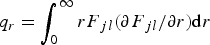 $q_r = \int_0^\infty {rF_{\,jl} (\partial F_{\,jl}/\partial r) {\rm d}r}$
,
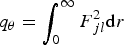 $q_{\rm \theta} = \int_0^\infty {F_{\,jl}^2 {\rm d}r} $
, and
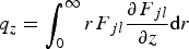 $q_z = \int_0^\infty {rF_{\,jl}\displaystyle{{\partial F_{\,jl}} \over {\partial z}}{\rm d}r} $
. Substituting Eqs. (4–6) into Eq. (3), the general dispersion relation becomes
 $$D(k,{\rm \omega} ) = 1 - \mathop \sum \limits_{\rm \alpha} \displaystyle{{{\rm \omega} _{{\rm p\alpha}} ^2} \over {k^2}} \int \displaystyle{{{\bi q}_{{\rm eff}}.(\partial f_{{\rm \alpha 0}}/\partial {\bi v})} \over {\omega - {\bi q}_{{\rm eff}} . {\bi v}}}d{\bi v} = 0.$$
The above equation is formally similar to the dispersion relation of the plane waves, except that the Landau resonance frequency in the presence of helical electric field occurs at
 $${\rm \omega} = kv_z + lq_{\rm \theta} v_{\rm \theta} \pm i(q_rv_r + q_zv_z).$$
In order to investigate the explicit effect of OAM on the obtained dispersion relation, we consider the approximation limit |q r |, |q z | << |lq θ|. In this limit, the modified resonance condition can be written as ω = kv z + lq θ v θ, in which the additional factor lq θ v θ indicates the effect of OAM of the twisted wave on the resonance frequency. Now, Eq. (8) can be reduced to
 $$D(k,{\rm \omega} ) = 1 - \mathop \sum \limits_{\rm \alpha} \displaystyle{{{\rm \omega} _{{\rm p\alpha}} ^2} \over {k^2}}\int\displaystyle{{lq_{\rm \theta} (\partial f_{{\rm \alpha 0}}/\partial v_{\rm \theta} ) + k(\partial f_{{\rm \alpha} 0}/\partial v_z)} \over {\omega - kv_z - lq_{\rm \theta} v_{\rm \theta}}} d{\bi v} = 0.$$
Or its expansion
 $$\eqalign{D(k,{\rm \omega} ) &= 1 - \mathop \sum \limits_{\rm \alpha} \displaystyle{{{\rm \omega} _{{\rm p\alpha}} ^{\rm 2}} \over {k^2}} \bigg\{\int \displaystyle{{(\partial f_{{\rm \alpha} 0}/\partial v_z)} \over {({\rm \omega} - lq_{\rm \theta} v_{\rm \theta} /k) - v_z}} {\rm d}{\bi v} \cr & \quad \matrix{+ \int \displaystyle{{(\partial f_{{\rm \alpha 0}}/\partial v_{\rm \theta} )} \over {(\omega \,-\, kv_z/lq_{\rm \theta} ) - v_{\rm \theta}}} {\rm d}{\bi v}\bigg\}}.} $$
Using the Plemelj formula, the above relation becomes
 $$\eqalign{ D(k,{\rm \omega} ) &= 1 + \mathop \sum \limits_{\rm \alpha} \displaystyle{{{\rm \omega} _{{\rm p\alpha}} ^2} \over {k^2}}\bigg\{{{\rm \cal P}}\int \left[ {\displaystyle{{(\partial f_{{\rm \alpha 0}}/\partial v_z)} \over {v_z - u_z}} + \displaystyle{{(\partial f_{{\rm \alpha 0}}/\partial v_{\rm \theta} )} \over {v_{\rm \theta} - u_{\rm \theta}}}} \right]{\rm d}{\bi v} \cr & \quad \matrix{ + i{\rm \pi} \int \left[ {\left( {\displaystyle{{\partial f_{{\rm \alpha 0}}} \over {\partial v_z}}} \right)\delta (v_z - u_z) + \left( {\displaystyle{{\partial f_{{\rm \alpha 0}}} \over {\partial v_{\rm \theta}}}} \right){\rm \delta} \left( {v_{\rm \theta} - u_{\rm \theta}} \right)} \right]{\rm d}{\bi v}\bigg\}},} $$
where
 ${{\rm \cal P}}$
is the principle value of integral, v
z
= (ω − lq
θ
v
θ)/k, and v
θ = (ω − lq
θ
v
z
)/k. To analyze the two-stream like instability of kinetic-model plasma equilibrium with the additional degree of freedom of temperature anisotropy, the equilibrium distribution function of shell species is considered as
 $$f_{{\rm \alpha 0}}(v_ \bot, v_z) = f_{{\rm \alpha 0}}(v_r,v_{\rm \theta} ){\rm \delta} (v_z - v_{{\rm 0\alpha}} ).$$
This temperature anisotropic distribution function represents streaming shell with the constant velocity v
z
= v
0α along the
 $\hat z$
-direction (
 $T_\parallel = 0$
), and with thermal distribution function in the plane normal to
 $\hat z$
, (T
⊥ ≠ 0). The perpendicular distribution function of the shell components, f
α0(v
⊥), are given by Maxwellian distribution function
 $$f_{{\rm \alpha 0}}(v_r,v_{\rm \theta} ) = \displaystyle{{m_{\rm \alpha}} \over {2{\rm \pi} k_{\rm B}T_{\rm \alpha}}} {\rm exp}\left[ { - \displaystyle{{m_{\rm \alpha} v_ \bot ^2} \over {2k_{\rm B}T_{\rm \alpha}}}} \right]. $$
Substituting Eqs. (14) and (13) into Eq. (12), the dispersion relation becomes
 $$\eqalign{D(k,{\rm \omega} ) &= 1 + \sum\limits_{\rm \alpha = e,P} \displaystyle{{\rm \omega}_{\rm p\alpha}^{\rm 2} \over k^2} \bigg\{{k^2 \over {\rm \omega}^{\rm 2}} \left( 1 + 2\nu_{0{\rm \alpha}} {k \over {\rm \omega}} + 3\nu_{0{\rm \alpha}}^2 {k^2 \over {\rm \omega}^{\rm 2}} \right) + {(lq_{\rm \theta})^2 \over ({\rm \omega} \,{\rm -}\, k\nu _{\rm 0\alpha})^2}\biggl( 1 + {3V_{\rm T\alpha}^2(lq_{\rm \theta})^2 \over 4({\rm \omega} \,{\rm -}\, k\nu_{\rm 0\alpha})^2}\bigg)\cr &\quad + {2i\sqrt {\rm \pi} \over V_{\rm T\alpha}^3} \left( {1 + \displaystyle{{k^2} \over {{(lq_{\rm \theta} )}^2}}} \right)\left( {\displaystyle{{{\rm \omega} \,{\rm -}\, k\nu _{{\rm 0\alpha}}} \over {lq_{\rm \theta}}}} \right)\exp \left[ { - \displaystyle{1 \over {V_{{\rm T\alpha}} ^2}} {\left( {\displaystyle{{{\rm \omega} \,{\rm -}\, k\nu _{{\rm 0\alpha}}} \over {lq_{\rm \theta}}}} \right)}^2}\right] \Biggr\}, }$$
in which
 $V_{{\rm T\alpha}} = \sqrt {(2k_{\rm B}T_{\rm \alpha} /m_{\rm \alpha} )} $
is the thermal speed of α-th species. This equation is formally different from the dispersion relation of the plane wave in the same configuration, where the additional contribution arises from the azimuthal term of the twisted modes. It should be noted that, in the limit of l → 0, Eq. (15) reduces to the familiar form of the plane wave dispersion relation. Using the normalized parameters defined as
 $$\eqalign{& {\rm \Omega} = \displaystyle{{\rm \omega} \over {{\rm \omega} _{{\rm pe}}}},\; \;K_z = \displaystyle{{kv_{{\rm 0e}}} \over {{\rm \omega} _{{\rm pe}}}},\; \;K_{\rm \theta} = \displaystyle{{lq_{\rm \theta} v_{{\rm 0e}}} \over {{\rm \omega} _{{\rm pe}}}},\;N_{\rm P} = \displaystyle{{\omega _{{\rm pP}}^2} \over {\omega _{{\rm pe}}^2}}, \cr & \;\;\;{\rm \beta} = \displaystyle{{v_{{\rm 0P}}} \over {v_{{\rm oe}}}},\; \;{\rm \alpha} _1 = \displaystyle{{V_{{\rm Te}}} \over {v_{{\rm 0e}}}},\;{\rm \alpha} _2 = \displaystyle{{V_{{\rm TP}}} \over {v_{{\rm 0P}}}}\comma} $$
the obtained dispersion relation (15) can be written in the normalized form as
 $$\eqalign{1 + & \displaystyle{1 \over {\Omega ^4}}\left[ {(1 + N_{\rm P})\Omega ^2 + 2K_z(1 + N_{\rm P}{\rm \beta} )\Omega + 3K_z^2 (1 + N_{\rm P}{\rm \beta} ^2)} \right] + \displaystyle{{K_{\rm \theta} ^2} \over {4K_z^2}} \cr \times & \left[ {3K_{\rm \theta} ^2 \left( {\displaystyle{{{\rm \alpha} _1^2} \over {{(K_z - \Omega )}^4}} + \displaystyle{{N_{\rm P}{\rm \alpha} _2^2 {\rm \beta} ^2} \over {{(\Omega - K_z{\rm \beta} )}^4}}} \right) + 4\left( {\displaystyle{1 \over {{(K_z - \Omega )}^2}} + \displaystyle{{N_{\rm P}} \over {{(\Omega - {\rm \beta} K_z)}^2}}} \right)} \right] + i\displaystyle{{2\sqrt {\rm \pi} (K_z^2 + K_{\rm \theta} ^2 )} \over {K_z^2 K_{\rm \theta} ^2}} \cr \times & \left[ {\displaystyle{{(\Omega - K_z)} \over {{\rm \alpha} _{\rm 1}^3}} \exp \left( {\displaystyle{{ - {(\Omega - K_z)}^2} \over {K_{\rm \theta} ^2 {\rm \alpha} _1^2}}} \right) + \displaystyle{{N_{\rm P}(\Omega - {\rm \beta} K_z)} \over {{\rm \beta} ^2{\rm \alpha} _2^2}} \exp \left( { - \displaystyle{{{(\Omega - {\rm \beta} K_z)}^2} \over {{\rm \beta} ^2{\rm \alpha} _2^2 K_{\rm \theta} ^2}}} \right)} \right] = 0.} $$
As can be seen, this relation is difficult to be solved analytically, so in the next section the numerical method will be employed to analyze the instability growth rate of the twisted modes.
3. NUMERICAL RESULTS AND DISCUSSION
In this section, the numerical method has been employed to solve the normalized dispersion relation (16) by considering the charge and current neutralization conditions as n e0 = n P0 + n i0, and n e0 v e0 = n P0 v P0 + n i0 v i0, respectively. Let us assume the unperturbed velocity of the plasma shell be v e0 = v P0 = v 0.
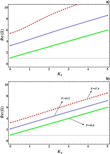
Figure 1 represents the variation of normalized real frequency [Re(Ω)] of twisted waves as a function of normalized wave number K z for the chosen system parameter values β = 1, N P = 0.5, K θ = 2, and α1 = α2 = 1/2, 3/2, 5/2 in Figure 1(a), and β = 1, N P = 0.5, α1 = α2 = 1, and K θ = 1, 2, 3 in Figure 1(b). As seen in Figure 1(a), for fixed value of azimuthal wave number, increasing the ratio of α(= α1 = α2) increases the slope of curves and so causes to increment of the group velocity of twisted waves. As well as, Figure 1(b) shows that for fixed value of normalized parameter α, the twisted waves group velocity increases very slowly (not so considerable) by the azimuthal wave number.
The variation of normalized real frequency [Re(Ω) = (ω/ωpe)] of twisted waves as a function of normalized longitudinal wave number (K z = kv 0e/ωpe) for β = 1, N P = 0.5 and (a) K θ = 2, α1 = α2 = 1/2 (solid green curve), α1 = α2 = 3/2 (dotted blue curve), α1 = α2 = 5/2 (dashed red curve), and (b) α1 = α2 = 1, K θ = 1 (solid green curve), K θ = 2 (dotted blue curve), and K θ = 3 (dashed red curve). γ is the slope of curves.

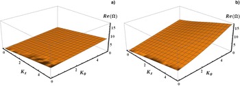
The effect of increasing of the parameter α on the variation of [Re(Ω)] for twisted waves is illustrated three dimensionally in Figure 2 for chosen quantities β = 1, N P = 0.5, α1 = α2 = 1/2 in Figure 2(a), and β= 1, N P = 0.5, α1 = α2 = 3/2 in Figure 2(b). We see that in Figure 2(a) and 2(b), increasing the longitudinal and azimuthal wave number increases the real part of frequency (phase velocity of wave). By comparing these two figures, it can be concluded that the phase and group velocities are enhanced by increasing the parameter α.
The 3D view of normalized real frequency of twisted waves in terms of K z and K θ for (a) α1 = α2 = 1/2 and (b) α1 = α2 = 3/2.

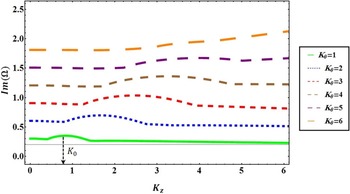
The effect of angular wave number on the instability of the excited twisted waves has been depicted in Figure 3. This figure exhibits the variation of normalized growth rate [Im(Ω)] versus normalized longitudinal wave number (K z ) for several values of K θ ranging from K θ = 1 to K θ = 6 with keeping constant the other parameter values (α, β, and N p). As seen clearly, for each given K θ and any arbitrary K z the growth rate curves show a non-zero value and a little bump around the specified wave number K 0, called the critical wave number.
The normalized growth rate as a function of normalized longitudinal wave number for fixed values of α = 1/2, β = 1, N P = 0.5 and different value of K θ.

The critical wave number as well as the band width of the bumps increase with increasing K θ. Moreover, for fixed value of longitudinal wave number, the growth rate dramatically increases with azimuthal wave number.
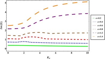
Figure 4 shows the variation of normalized growth rate [Im(Ω)] versus normalized longitudinal wave number (K z ) for different values of α ranging from α = 0.2 to α = 1.4 with keeping constant quantities of K θ, β, and N p. In Figure 4, for a specified value of K z , the growth rate increases by increasing α. On the other hand, for α<1 the width and height of the bump of the growth rate curves increase by enhancing the values of α, and then the growth rate eventually saturates after the turning point. While for α>1 in which the thermal speed of electrons and positrons is larger than the shell velocity, the instability of twisted waves enhances and, consequently, the system will be highly unstable on the electron time scale. It seems that the reason of this behavior arises from the enhancement of the free energy originating from increment of the thermal motion of shell components.
The normalized growth rate as a function of normalized longitudinal wave number for fixed values of K θ = 3, β = 1, N P = 0.5 and different value of α.

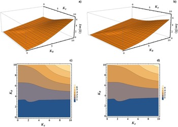
The dependence of the growth rate of twisted wave in our system on the magnitude of N p is demonstrated in Figure 5. In this figure, the normalized growth rate as a function of normalized longitudinal and azimuthal wave number is shown three dimensionally for N p = 0.1 and 0.5 with corresponding contour plot of them. Comparing Figure 5(a) and 5(b), it is deduced that when the concentration of positron in the system is diminished the growth rate of the twisted mode is enhanced. In addition to, the contour plot of these figures [Figure 5(c) and 5(d)] show that for a fixed value of K z the variations of growth rate are more than those for a fixed value of K θ. In other words, azimuthal wave number has a more important role on the growth rate than the longitudinal wave number.
The 3D view of normalized growth rate as a function of normalized longitudinal and azimuthal wave number for (a) N p = 0.1, α = 1/2, β = 1, and (b) N P = 0.5, α = 1/2, β = 1 with a corresponding contour plots of them.

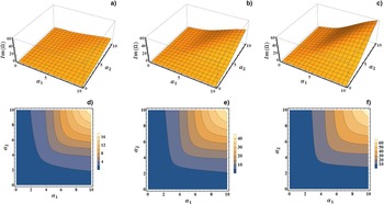
Finally, we close this investigation by plotting the three-dimensional (3D) view of normalized growth rate as a function of α1 and α2 to show the role of K θ = 1, 2, 3 in the variation of growth rate for K z = 1, N P = 0.5, and β= 1. From Figure 6 it is concluded that, by increasing the value of K θ the amount of growth rate increases. Furthermore, for the fixed values of K z and K θ the growth rate increases with α1 and α2. Also, Figure 6(d), 6(e), and 6(f) which are the corresponding contour plots of Figure 6(a), 6(b), and 6(c), respectively, display that only for a small values (arbitrary value) of α1 and arbitrary value (small values) of α2 the amount of growth rate are approximately constant. Of course this interval of constant growth rate increases by increasing the value of K θ.
The 3D view of normalized growth rate as a function of α1 = V Te/v 0e and α2 = V TP/v 0P with a corresponding contour plots for (a, d) K θ = 1, K z = 1, β = 1, N P = 0.5, (b, e) K θ = 2, K z = 1, β = 1, N P = 0.5, (c, f) K θ = 3, K z = 1, β = 1, N P = 0.5.

4. SUMMARY AND CONCLUSION
In this paper, the kinetic approach has been used to study the instability of the twisted wave carrying OAM in an unmagnetized collisionless plasma system containing of e–p shell drifting through the moving ion background. Considering the electrostatic potential in the paraxial limit and employing the LG perturbed distribution function, the Vlasove–Poisson equation has been solved to derive the dispersion relation of perturbed twisted waves in the given temperature anisotropic system. Based on the numerical analysis, the behavior of instability growth rate of twisted modes has been investigated in detail. It has been found that the instability of the electrostatic twisted wave increases by angular mode number, and this increment is more considerable for high values of shell temperature. Moreover, the growth rate diminishes with enhancement of the positron concentration in the system. In addition to, the results show that the impact of azimuthal wave number on the increasing of the growth rate is larger than longitudinal wave number. Our results can be applied to experimental processes such as in inertial confinement fusion where the interaction of high-power laser with matter produces an e–p shells (Chen et al., Reference Chen, Nakai, Sentoku, Arikawa, Azechi, Fujioka, Keane, Kojima, Goldstein, Maddox, Miyanaga, Morita, Nagai, Nishimura, Ozaki, Park, Sakawa, Takabe, Williams and Zhang2013), and to astrophysical systems like as gamma-ray burst in the presence of e–p winds (Geng et al., Reference Geng, Wu, Huang, Li and Dai2016).
APPENDIX A: L–G POTENTIAL AND ELECTRIC FIELD
For electrostatic twisted modes propagating along the
 $\hat z$
-axis with slowly varying amplitude, the potential function can satisfy the paraxial equation as
 $$\left( {\nabla _ \bot ^2 + 2ik_z\displaystyle{\partial \over {\partial z}}} \right){\rm \phi} ({\bi r},t) = 0.$$
Here
 $\nabla _ \bot ^2 = (1/r)\partial /\partial r\left( {r\partial /\partial r} \right) + \left( {1/r^2} \right)\partial ^2/\partial {\rm \varphi} ^2$
is the perpendicular component of Laplacian operator in the cylindrical coordinates. By solving Eq. (A1), one can obtain the LG potential for system which is described by superposition of LG functions as follows:
 $${\rm \phi} ({\bi r},t) = \mathop \sum \limits_{\,jl} \tilde {\rm \phi} _{\,jl}F_{\,jl}(r,z){\rm exp}(il{\rm \theta} + ik_{\rm z}z - i{\rm \omega} t)$$
and
 $$F_{\,jl}(r,z) = \displaystyle{1 \over {2\sqrt {\rm \pi}}} \left\{ {(l + j)!/j!} \right\}^{\displaystyle{1 \over 2}}X^{\left \vert l \right \vert} L_j^{\left \vert l \right \vert} {\rm exp}\left( { - \displaystyle{X \over 2}} \right).$$
where
 $\tilde {\rm \phi}_{\,jl}$
is the mode amplitude, j(= 0, 1, 2, …) and l(= 0, ± 1, ± 2, …) are the radial and angular mode numbers, respectively. Also X = r
2/w(z)2, w(z) being the beam waist, θ is the azimuthal angle, and Laguerre polynomials are given as:
 $$L_j^{\left \vert l \right \vert} (X) = \displaystyle{{{\rm exp}(X)} \over {Xj!}}\displaystyle{{d^j} \over {dX^j}}\left[ {X^{l + j}\exp ( - X)} \right].$$
Also, the LG modes satisfy the orthogonality conditions
 $$F_{{\,j}^{\prime}{l}^{\prime}}{\rm \vert} F_{\,jl} = \int_0^{2{\rm \pi}} {\int_0^\infty {d{\rm \theta}}} \;r{\rm d}rF_{{\,j}^{\prime}{l}^{\prime}}F_{\,jl}e^{i\left( {l - {l}^{\prime}} \right){\rm \theta}} = {\rm \delta} _{\,j{\,j}^{\prime}}{\rm \delta} _{l{l}^{\prime}}.$$
Having the LG potential and using
 ${\bi E} = - \nabla {\rm \phi} $
, we can calculate the components of electric field in the cylindrical coordinates. The electric field components given by
 $$E_r = - \displaystyle{{{\rm \phi} ({\bi r},t)} \over {F_{{ jl}}}}\displaystyle{{\partial F_{\,jl}} \over {\partial r}},$$
 $$E_{\rm \theta} = - i\displaystyle{{l{\rm \phi} ({\bi r},t)} \over r},$$
 $$E_{\rm z} = - \left( {ik_z + \displaystyle{1 \over {F_{\,jl}}}\displaystyle{{\partial F_{\,jl}} \over {\partial z}}} \right){\rm \phi} ({\bi r},t).$$
This equations show that the electric field lines are not straight lines along the z-direction as in ordinary plane wave solutions, but are showing helical structures. With consider the
 ${\bi k}_{{\rm ef}} = \left\{ {( - i/F_{\,jl})\left( {\partial F_{\,jl}/\partial r} \right)} \right\}\hat e_r + \left\{ {l/r} \right\}\hat e_{\rm \theta} + \left\{ {k_{\rm z} - (i/F_{\,jl}) \left( {\partial F_{\,jl}/\partial z} \right)} \right\}\hat e_z$
, the electric field can be represented as
E
= −i
k
ef
ϕ(r, φ, z).