D.c. electrical conductivity of Sea ice

Sea ice is an inhomogeneous composite of pure ice, brine, air and, at low temperatures, precipitated Salts. a number of authors have reported results of in Situ conductivity (or resistivity) measurements on arctic and antarctic Sea ice. Reference Thyssen, Kohnen, Cowan and TimcoThyssen and others (1974), Reference KohnenKohnen (1976), Reference TimcoTimco (1979) and buckley and others (1986) report results of traditional d.c. resistivity measurements on Sea ice. Reference Morey, Kovacs and CoxMorey and others (1984) conducted time-domain reflectometry (tdr) measurements using ‘ladders’ of transmission lines frozen into growing arctic Sea ice, from which they were able to determine the d.c. conductivity. Reference Becker, Echert and G.B.Becker and others (1992) determined in Situ Sea-ice conductivity using high-frequency em methods (8–16 mhz) via measurements of the radiation resistance of a circular loop antenna placed on the Surface of the ice.

Columnar Sea ice exhibits a preferred fabric, with the orientation of the c axes of the ice crystals predominantly horizontal, perpendicular to the direction of Sea-ice growth (Reference TimcoTimco, 1979; Reference Weeks, Ackley and UntersteinerWeeks and ackley, 1986). brine inclusions within the Sea ice occur as thread-like cells arranged in thin, vertically oriented layers. the Shape of the brine cells is temperature-dependent: the cells are needle-shaped at low temperatures, but become disc-shaped at very warm temperatures (Reference TimcoTimco, 1979). as the Sea ice grows thicker, the entrapped brine drains out under gravity, forming vertically aligned drainage tubes. drainage tube diameters are typically 0.1–1 cm, although diameters of up to 10cm have been reported (Reference Weeks, Ackley and UntersteinerWeeks and ackley, 1986). under certain temperature conditions, the drainage tubes may extend through the entire thickness of the Sea ice (Reference GoldenGolden, 2001).

The vertical orientation of both the brine cells and drainage tubes imparts a Strong conductivity anisotropy to the Sea ice, with the bulk conductivity in the vertical direction being higher than that in the horizontal direction (Reference Thyssen, Kohnen, Cowan and TimcoThyssen and others, 1974). Reference Watson and BarkerThyssen and others (1974) verified the presence of this conductivity anisotropy in Situ, by making direct measurements of the horizontal and vertical conductivities in the walls of a pit excavated in thick, undeformed arctic Sea ice. buckley and others (1986) detected a Similar anisotropy in first-year antarctic Sea ice.

Resolution of horizontal and vertical conductivities

Our wenner Sounding and offset wenner azimuthal data Show that the Sea-ice conductivity is horizontally isotropic, but that the vertical conductivity is higher than the horizontal conductivity. this type of electrical Structure is referred to as ‘transversely isotropic’ in the geophysical literature. Reference MailletMaillet (1947) has Shown that a transversely isotropic layer of thickness t _a, with conductivities of σ _h and σ _v in the horizontal and vertical directions respectively, yields an identical d.c. Sounding response to an isotropic layer of thickness t = (σ _h/σ _v)^1/2 t _a and conductivity σ _m=(σ _h σ _v)^1/2. this equivalence is illustrated in figure 3. the quantity f=(σ _h/σ _v)^1/2 = t/t _a is the coefficient of anisotropy. in typical Situations, it is not possible to identify the presence of this type of anisotropy on the basis of Surface geoelectrical Sounding data. in the Sea-ice case, the difference between the interpreted thickness (t) and drilled thickness (t _a) reveals the presence of the anisotropy: the ratio t/t _a allows us to directly determine f and hence to resolve σ _h and σ _v independently, Since

Fig. 3.

Equivalent transversely isotropic (left) and isotropic (right) 1-D d.c. geoelectrical models. For the anisotropic case, σ _v and σ _h are the conductivities in the vertical and horizontal directions respectively, and t_a is the layer thickness. In the isotropic model, σ _m and t are the equivalent upper-layer conductivity and thickness respectively. In both models, the conductivity of the bottom layer (sea water) is isotropic.

(2)

σ _v is easily obtained once σ _h has been determined as above. Reference Thyssen, Kohnen, Cowan and TimcoThyssen and others (1974) calculated horizontal and vertical conductivities using the Same approach.

We have performed a detailed analysis of five of our geoelectrical Soundings for which drilling revealed the Sea-ice thickness to be essentially constant below the electrode array, and where our assumed 1-d interpretation model was appropriate. at the other field Sites, drilled Sea-ice thickness below the electrode array varied by tens of centimetres to metres, and it was not possible to assume that the underestimation of Sea-ice thickness was Solely due to conductivity anisotropy. for each of the Soundings on level Sea ice, an adequate fit to the observed data was obtained using a three-layered model containing a near-surface conductive layer (Reference Thyssen, Kohnen, Cowan and TimcoThyssen and others, 1974; Reference Buckley, Staines and RobinsonBuckley and others, 1986). the Smallest electrode Spacing used for the field measurements (a = 0.1 m; fig. 1a) was too large to allow the conductivity and thickness of the uppermost layer to be determined (buckley and others, 1986). however, an equivalence analysis of the data indicates that the upper layer is at most a few centimetres thick. all of the equivalent models for the upper conductive layer have an identical longitudinal conductance (conductivity–thickness product); the calculated conductance of the layer, S ₁, is given in table 1.

Table 1.

Results of in Situ d.c. conductivity measurements on level East Antarctic pack ice. Measurements were made during the period 26 September–20 October 2003. Temperature (T) was measured at the Snow–sea-ice interface; Sea-water temperature was ≈–1.8˚C. t _a is the mean drilled thickness of the Sea ice. t and σ _m are the Sea-ice thickness and Second-layer conductivity interpreted from d.c. geoelectrical data assuming a layered isotropic model, and S ₁ is the conductance (conductivity–thickness product) of the first layer. f is the coefficient of anisotropy, and σ _h and σ _v are the approximate horizontal and vertical conductivities, calculated as described in the text

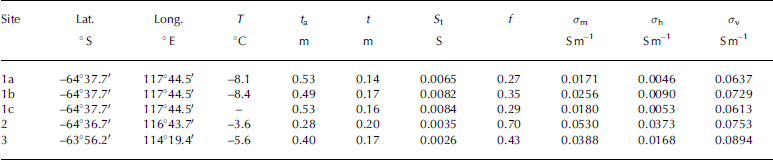
The Small thickness of the upper conductive layer means that the Sea-ice thickness interpreted from the geoelectrical Sounding data is essentially equal to the thickness of the Second layer of the model. Subject to this assumption, it is possible to calculate f and hence to determine approximate horizontal and vertical conductivities for the Second model layer, which represents the bulk of the Sea ice. the results of these calculations are Summarized in table 1 and plotted in figure 4.

Fig. 4.

Graph of in Situ Sea-ice conductivity and coefficient of anisotropy vs drilled thickness for five d.c. geoelectrical Soundings on level Sea ice in East Antarctica. σ _h and σ _v are the interpreted Sea-ice conductivities in the horizontal and vertical directions respectively. σ _m is the conductivity of the equivalent isotropically conductive layer and is equal to the geometric mean of the horizontal and vertical conductivities.

The conductivities listed in table 1 are consistent with those from other published in Situ data. Reference Thyssen, Kohnen, Cowan and TimcoThyssen and others (1974) measured horizontal and vertical conductivities in the wall of a pit excavated in arctic Sea ice, and obtained σ _h = 0.01 Sm^–1 and σ _v = 0.063 Sm^–1. Reference Buckley, Staines and RobinsonBuckley and others (1986) noted the presence of conductivity anisotropy in antarctic Sea ice of thickness 1.35–1.75 m, but did not determine σ _h and σ _v. based on their published data, we have calculated values of σ _h between 0.002 and 0.01 Sm^–1 and σ _v between 0.01 and 0.034 Sm^–1. the in Situ tdr measurements of Reference Morey, Kovacs and CoxMorey and others (1984) measured horizontal conductivities for 1.4m thick first-year arctic Sea ice of between 0.009 Sm^–1 near the top of the Sea ice and 0.13 Sm^–1 near the more porous base. it Should be noted that conductivities interpreted from d.c. geoelectrical data assign bulk horizontal and vertical conductivities to the Sea ice and cannot be directly compared with the results of Reference Morey, Kovacs and CoxMorey and others (1984) which were made at a much Smaller horizontal Scale (∽1 cm) at a range of depths within the Sea ice.

Comparison with Archie’s law

In the absence of in Situ data, a first approximation to the Sea-ice conductivity can be estimated from core Samples using the empirical Reference ArchieArchie’s law (archie, 1942; Reference Haas, Gerland, Eicken and MillerHaas and others, 1997) which relates the bulk conductivity σ of the Sea ice to its porosity (assumed equivalent to the brine volume, v _b) and the conductivity of the brine, σ _b:

(3)

Values for the constant m, appropriate to Sea ice, have been determined by thyssen and others (1974) and Reference Morey, Kovacs and CoxMorey and others (1984). thyssen and others (1974) obtained m = 2.2, while morey and others (1984) obtained m = 1.55 near the top of the Sea ice, and 1.75 near the base. the change in the value of m with depth was attributed to a change in Structure of the Sea ice from a vertical c-axis orientation near the top of the ice to a predominantly horizontal c-axis orientation near the base. Reference Haas, Gerland, Eicken and MillerHaas and others (1997), Reference Worby, Griffin, Lytle and MassomWorby and others (1999) and Reference Tateyama, Uto, Shirasawa, Enomoto, Chung, Izumiyama, Sayed and HongTateyama and others (2004) all assumed a value of m = 1.75 for their archie’s law calculations.

Calculation of v _b requires Salinity and temperature measurements along the length of the core. the Salinity measurement requires that the core Sections be melted, which has the important consequence of destroying the Structural fabric of the Sea ice, and hence any anisotropy. the archie’s law conductivities can also be affected by loss of brine when the core is extracted from the Sea ice.

We have calculated v _b using the method of Reference Cox and WeeksCox and weeks (1983). the brine conductivity σ _b for each core interval was calculated from the measured temperature using an equation given by Reference Stogryn and DesargantStogryn and desargant (1985):

(4)

Where T is the temperature in degrees celsius and σ _b is in Sm^–1.

figures 5 and 6 Show Salinity and temperature measurements for the cores from Sites 1a and 2, as well as bulk conductivities determined using archie’s law for two published values of m. these cores correspond to the Sites with the Smallest (site 1a) and largest (site 2) coefficients of anisotropy determined from the wenner d.c. Soundings. horizontal and vertical conductivities determined from the wenner Sounding data are indicated by the horizontal dashed lines in figures 5b and 6b. the archie’s law conductivities calculated for m = 1.75 are generally a better approximation to σ _v than σ _h. we have determined bulk core conductivities by Summing the conductances (conductivity times length) of each core Segment and dividing by the total length of the core. assuming m = 1.75, bulk conductivities calculated for cores 1a and 2 are 0.063 and 0.098 Sm^–1. for m = 2.2, bulk conductivities are 0.023 Sm^–1 (core 1a) and 0.041 Sm^–1 (core 2).

Fig. 5.

(a) Salinity and temperature profiles measured on a Sea-ice core from Site 1a (Table 1). (b) Bulk Sea-ice conductivity computed from the data in (a) using Archie’s law, for different values of the exponent m. The horizontal dashed lines denote the horizontal (σ _h) and vertical (σ _v) conductivities determined from interpretation of the in Situ d.c. geoelectrical Sounding data, as described in the text.

Fig. 6.

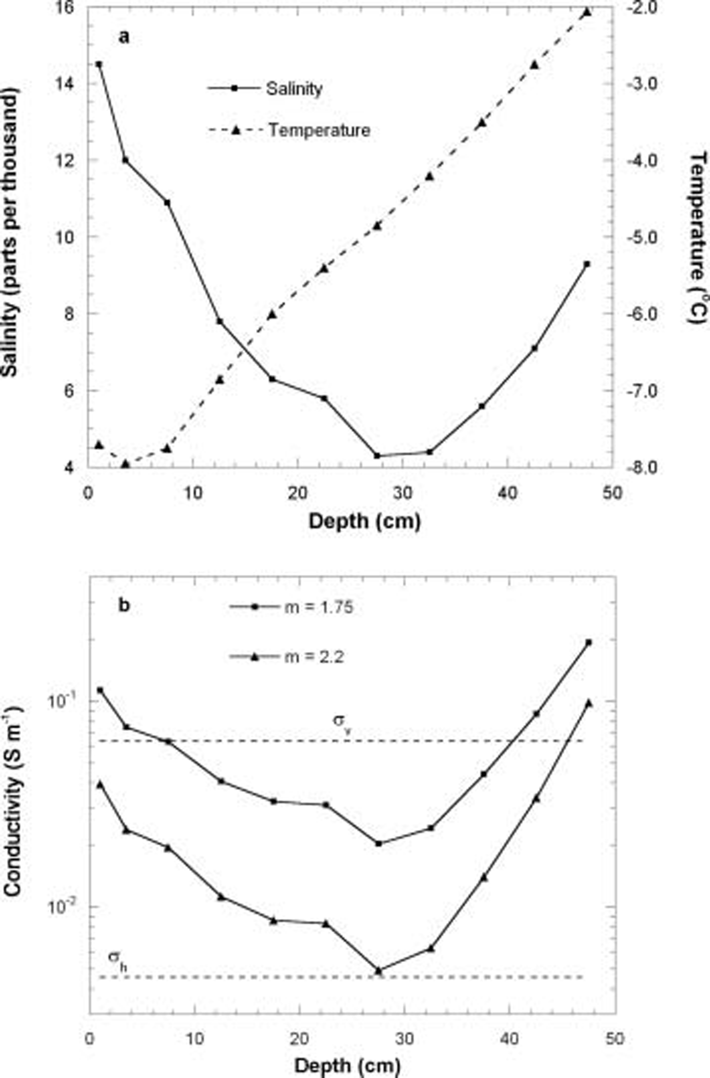
(a) Salinity and temperature profiles measured on a Sea-ice core from Site 2 (Table 1). (b) Bulk Sea-ice conductivity computed from the data in (a) using Archie’s law, for different values of the exponent m. The horizontal dashed lines denote the horizontal (σ _h) and vertical (σ _v) conductivities determined from interpretation of the in Situ d.c. geoelectrical Sounding data.

The data Shown in table 1 indicate coefficients of anisotropy (f) for east antarctic pack ice of 0.27–0.7. thyssen and others (1974) obtained f = 0.26 for undeformed Sea ice, and found deformed Sea ice to be isotropic (f = 1) as a result of destruction of the preferred fabric in undeformed Sea ice. Reference Buckley, Staines and RobinsonBuckley and others (1986) obtained a coefficient of anisotropy of 0.5 for undeformed first-year antarctic Sea ice.

figure 4 Shows a consistent increase in the coefficient of anisotropy with decreasing Sea-ice thickness, although it is difficult to Say whether this is a real trend, given the limited number of measurements. congelation (columnar) Sea ice could be expected to Show Strong electrical anisotropy in comparison with frazil ice. although no Structural description was available for core 1a, three cores taken from the Same floe, and of almost identical thickness, contained an average of 75% congelation ice, with the uppermost Sections of all cores being composed of frazil and Snow ice. core 2 was composed of 58% congelation ice, with the uppermost Section of the core being composed of frazil and Snow ice. Site 1 Shows the Strongest anisotropy, consistent with its higher content of congelation ice, although the difference in congelation ice contents Seems too minor to explain the large difference in the coefficient of anisotropy at the two Sites. the weaker anisotropy at Site 2 could also be due to the relatively high temperature of the Sea ice at this Site. table 1 Suggests a general positive correlation between Sea-ice temperature and the coefficient of anisotropy. this may imply an increase in the lateral interconnection between the brine cells with increasing temperature.

Implications for airborne EM Soundings of Sea-ice thickness

An arbitrarily oriented em transmitter located on or above the Surface of a layered earth will induce current flow only in the horizontal plane. em measurements over undeformed, transversely isotropic Sea ice are therefore Sensitive only to the horizontal conductivity. this has been formally demonstrated for the case of a transversely isotropic half-space by Reference SinhaSinha (1968), but the result generalizes to the case of a multilayered earth (Reference Yin and FraserYin and fraser, 2004).

We have conducted a theoretical investigation of the Sensitivity of the awi hem-bird System to Sea-ice conductivity. the awi hem-bird is a two-frequency System which employs a horizontal coplanar transmitter–receiver geometry. data are acquired at frequencies of 3680 and 112 khz, with transmitter–receiver Separations of 2.77 and 2.05m respectively. at each frequency, the receiver measures the components of the Secondary magnetic field both in-phase and out-of-phase with the primary magnetic field of the transmitter. the Secondary fields are expressed as parts per million (ppm) of the primary field. the altitude of the System above the Sea ice is monitored using a laser altimeter. a full description of the System, and the practical techniques used to recover Sea-ice thickness from the measured data, are given in Reference Haas, Edeler, Schürmann, Lobach and SengpielHaas and others (2002) and Reference Pfaffling, Haas and ReidPfaffling and others (2004).

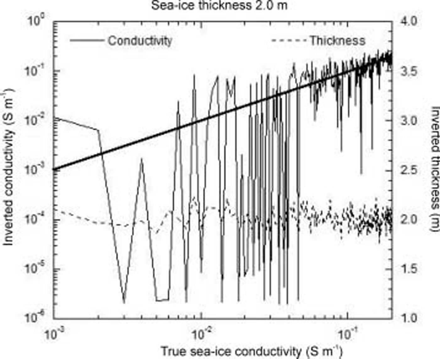
We have calculated the theoretical awi hem-bird response of a Suite of two-layer 1-d models, in which the Sea-ice conductivity was varied while the Sea-ice thickness and Sea-water conductivity were held constant. the results of one Such modelling exercise are Shown in figure 7. in this case, the two-layered model consisted of a 2 m thick layer of Sea ice over Sea water of conductivity 2.77 Sm^–1. the Sea-ice conductivity used for the model calculations ranged from 0.001 to 0.2 Sm^–1 in increments of 0.001 Sm^–1. random noise was added to the in-phase and out-of-phase components of the model response at each frequency. noise levels were derived from data recorded during the 2003 field program. noise was assumed to be gaussian, with Standard deviations of 6.38 and 5.81 ppm for the in-phase and out-of-phase components at 3680 hz, and 9.24 and 13.42 ppm for the in-phase and out-of-phase components at 112 khz. the noise-contaminated data were then interpreted using a 1-d least-squares inversion program in order to attempt to Simultaneously recover both Sea-ice conductivity and thickness. the inversion process also assumed a two-layered model, in which the Sea-ice thickness and conductivity were allowed to vary, while the Sea-water conductivity was held fixed at 2.77 Sm^–1. this is Similar to field Situations, where the Sea-water conductivity is usually known from independent measurements Such as conductivity–temperature–depth Soundings. the Starting model for the inversion assumed a Sea-ice thickness of 4m, and conductivity of 0.1 Sm^–1. the Sea-ice conductivity and thickness determined by inversion of the noisy Synthetic data are Shown in figure 7. the true Sea-ice thickness of 2.0 m is recovered quite well, with a maximum error of 12%. however, the Sea-ice conductivity is very poorly constrained, particularly for model conductivities of <0.05 Sm^–1. the recovered conductivity exhibits variations of up to two orders of magnitude even for model Sea-ice conductivities above 0.05 Sm^–1. figure 7 Shows that, given practical noise levels, the awi hem-bird System is insensitive to the Sea-ice conductivity, even over Sea ice of thickness 2 m.

Fig. 7.

Sea-ice conductivity and thickness recovered by inversion of noise-contaminated Synthetic airborne EM data, for a Suite of models in which the Sea-ice thickness and Sea-water conductivities were held fixed at 2m and 2.77 Sm^–1 respectively, while the Sea-ice conductivity varied between 0.001 and 0.2 Sm^–1. The heavy diagonal line denotes a 1 : 1 relationship between the true and inverted Sea-ice conductivities. The height of the airborne EM System was assumed to be 15 m for all model calculations. A full description of the model parameters and noise levels is given in the text.

We have found the Sensitivity of the airborne em response to Sea-ice conductivity to be even lower over Sea ice <2m thick. our model calculations Suggest that, given the practical noise limits of the awi hem-bird System, the conductance of the Sea ice (σ _h times drilled thickness) must be around 0.25–0.4 S before the Sea-ice conductivity can be recovered from the em data with any degree of confidence. this is Supported by further model calculations (not Shown), which indicate that level Sea ice of conductivity 0.05 Sm^–1 must be in excess of 5 m thick before the conductivity can be reliably recovered (<10% error) from inversion of practical awi hem-bird data.

The maximum Sea-ice conductance determined from our in Situ measurements was approximately 0.014 S, including the contribution from the conductive near-surface layer (table 1). the horizontal conductivities determined from our in Situ d.c. Sounding data are So low that the effects of Sea-ice conductivity on awi hem-bird data can generally be ignored over level Sea ice in the east antarctic, where the modal Spring thickness is typically around 0.5 m (Reference Worby, Massom, I., Lytle, Heil and JeffriesWorby and others, 1998). this may not be the case during the late Summer, where high temperatures result in high brine volumes and a Significantly increased bulk Sea-ice conductivity (Reference HaasHaas, 1998).

Conclusions

Airborne em measurements over transversely isotropic Sea ice are Sensitive only to the conductivity in the horizontal direction. over level Sea ice, it is possible to determine approximate horizontal and vertical conductivities from d.c. geoelectrical Sounding data. five wenner-array geoelectrical Soundings on level east antarctic pack ice during Spring 2003 have yielded average horizontal and vertical conductivities of 0.017 and 0.073 Sm^–1 respectively. these conductivities compare well with those from other in Situ measurements reported in the literature. the widely used form of archie’s law (with exponent m = 1.75) appears to Significantly overestimate the horizontal conductivity of the Sea ice.

High-frequency airborne em data from the awi hem-bird System have been Shown to be insensitive to the electrical conductivity of undeformed east antarctic Sea ice, given the practical noise levels measured during the September 2003 field Surveys. a much earlier field-based Study of airborne em measurements of Sea-ice thickness (Reference Kovacs and HolladayKovacs and holladay, 1990) reached a Similar conclusion for arctic Sea ice. the insensitivity of the System to Sea-ice conductivity was attributed to temperature-related drift affecting both the System electronics and transmitter frequency. although the awi hem-bird contains internal calibration coils which allow in-flight calibration factor adjustments during high-altitude drift correction of the data, further reductions in the noise levels (possibly coupled with an increased maximum transmitter frequency) are required before Sea-ice conductivity measurements will be possible over the relatively thin Sea ice typical of the east antarctic.