1 Introduction
To increase the energy efficiencies and to achieve energy savings for various thermo-fluids devices, the control of fluid flow and associated transport processes is of fundamental importance. For example, heat exchangers are widely used for exchanging heat between two fluid media in industrial processes, and their performances play critical roles in determining the overall efficiencies. Heat transfer between two fluids generally occurs across a heat transfer surface, and this inevitably causes two irreversible losses due to wall skin friction and heat transfer resistance. So far, significant efforts have been made to simultaneously minimize the two irreversible losses arising within a fluid domain by enhancing heat transfer with less wall skin friction. According to the Reynolds analogy (Bejan Reference Bejan2013), however, achieving such dissimilar heat transfer enhancement is quite challenging due to the inherent similarity between the governing equations of momentum and heat transfer.
Meanwhile, it has been widely known that the scalar diffuses relatively faster than the momentum in turbulent shear flows (Fiedler Reference Fiedler1975). Experimental measurements in a turbulent boundary layer revealed dissimilarity between the streamwise velocity and temperature fluctuations especially at high frequencies (Fulachier & Dumas Reference Fulachier and Dumas1976), so that their correlation gradually decays with increasing the distance from the wall (Antonia, Krishnamoorthy & Fulachier Reference Antonia, Krishnamoorthy and Fulachier1988). Recent direct numerical simulations (DNSs) of turbulent Couette and channel flows (Pasinato Reference Pasinato2011; Zhou, Klewicki & Pirozzoli Reference Zhou, Klewicki and Pirozzoli2019) also show non-negligible dissimilarity even in an ideal situation where the transport equations and boundary conditions for streamwise momentum and temperature are similar. The above results suggest that the Reynolds analogy does not hold perfectly even in canonical turbulent flows, and the dissimilarity between turbulent heat and momentum transfer could be further enhanced through flow control.
There exist plenty of studies focusing exclusively on reducing the skin-friction drag in wall-bounded turbulent flows. Drag reduction techniques proposed so far can be broadly classified into passive or active control depending on the energy expenditure for flow control (Gad-el-Hak Reference Gad-el-Hak2006). The active control requires an external power input and it generally yields higher control performances than the passive control. The active control can be further classified into two subcategories: reactive and predetermined controls. While the reactive control is flexible due to the combined use of actuators and sensors, it generally makes the control system very complex. In contrast, the predetermined control has the advantage that it applies a relatively simple control input (usually characterized by a harmonic function in space and/or time) without the need for sensing the instantaneous flow state.
Streamwise travelling wave-like wall blowing and suction, which is considered in the present work, is a typical example of the predetermined control techniques. It has two distinct mechanisms of drag reduction. The first one is the so-called streaming (or pumping) effect, which causes a net mass flux in the opposite direction to the applied travelling wave even without imposing a pressure gradient (Hoepffner & Fukagata Reference Hoepffner and Fukagata2009). Since the control input itself assists to drive the flow downstream, the external pressure gradient for achieving a given flow rate can be reduced. This effect exists for both laminar and turbulent flows. Indeed, properly designed upstream travelling waves (UTW) were found to achieve significant drag reduction and even sub-laminar drag in a turbulent channel flow (Min et al. Reference Min, Kang, Speyer and Kim2006). By analysing the phase relationship between the fluctuating velocity components, Mamori, Fukagata & Hoepffner (Reference Mamori, Fukagata and Hoepffner2010) revealed that the viscous effect induces a near-wall phase shift between streamwise and wall-normal velocity fluctuations, and thus generates the Reynolds shear stress, which is the origin of the streaming effect. They also found that a varicose mode is more effective than a sinuous mode. Woodcock, Sader & Marusic (Reference Woodcock, Sader and Marusic2009) derived an asymptotic expression for an induced net flow due to the streaming effect and confirmed that the varicose mode is more effective.
The second mechanism is the stabilizing effect through interaction between the applied travelling wave-like control input and underlying wall turbulence. Obviously, it is present only in a turbulent flow. The stability analysis by Lee, Min & Kim (Reference Lee, Min and Kim2008) revealed that UTW destabilizes a turbulent flow, hence the drag reduction achieved by Min et al. (Reference Min, Kang, Speyer and Kim2006) is mostly caused by the streaming effect. Meanwhile, their analysis showed that streak amplification due to transient growth is significantly suppressed when a downstream travelling wave (DTW) is applied. It was later proved that significant drag reduction, and even relaminarization can be achieved using a DTW (Lieu, Moarref & Jovanović Reference Lieu, Moarref and Jovanović2010) when the parameters of the travelling wave are determined based on the receptivity analysis (Moarref & Jovanović Reference Moarref and Jovanović2010). A parametric study based on DNSs in this regard was carried out by Mamori, Iwamoto & Murata (Reference Mamori, Iwamoto and Murata2014). They identified the conditions for the parameters of DTW to relaminarize a fully developed channel flow at  $Re_{\unicode[STIX]{x1D70F}}=110$ and
 $300$.
Although the complex responses of skin-friction drag to various control inputs have been extensively investigated, studies considering their impacts on the thermal field and the dissimilarity between momentum and heat transfer are still limited. Suzuki, Suzuki & Sato (Reference Suzuki, Suzuki and Sato1988) and Inaoka, Yamamoto & Suzuki (Reference Inaoka, Yamamoto and Suzuki1999) considered a turbulent boundary layer disturbed by insertion of a cylinder and a square duct, respectively. They observed significant dissimilarity downstream of the obstacles. Matsubara, Miura & Ohta (Reference Matsubara, Miura and Ohta2015) also conducted DNSs of a turbulent channel flow with a spanwise rib, and the detailed mechanisms of dissimilarity caused by the spanwise rib were discussed based on flow visualization, statistics and spectral analyses. With respect to active control, dissimilarity caused by wall blowing from a spanwise slot in a turbulent boundary layer is considered in Kong, Choi & Lee (Reference Kong, Choi and Lee2001) and Araya, Leonardi & Castillo (Reference Araya, Leonardi and Castillo2008). Although the above studies clearly show the responses of the velocity and thermal fields to a disturbance are fundamentally different, they mostly focus on the local effects in the immediate downstream of the control region.
Based on their DNSs using travelling wave-like wall blowing and suction control input, Higashi, Mamori & Fukagata (Reference Higashi, Mamori and Fukagata2011) showed that it is possible to simultaneously achieve heat transfer augmentation and friction drag reduction by applying UTW for both laminar and turbulent channel flows. Kasagi et al. (Reference Kasagi, Hasegawa, Fukagata and Iwamoto2012) revisited the governing equations and boundary conditions for the velocity and thermal fields, and summarized the possible scenarios leading to the dissimilarity between the streamwise momentum and the temperature. Among them, they concluded that the fundamental difference between the divergence-free vector and the conservative scalar should yield a universal strategy for dissimilar heat transfer enhancement. Based on this idea, Hasegawa & Kasagi (Reference Hasegawa and Kasagi2011) and Yamamoto, Hasegawa & Kasagi (Reference Yamamoto, Hasegawa and Kasagi2013) achieved dissimilar heat transfer enhancement in a turbulent channel flow by applying suboptimal and optimal control theories, respectively. In both studies, the spatio-temporal distribution of the wall transpiration is optimized so as to minimize a cost functional which is given as a linear weighted sum of the cost of wall friction and the merit of heat transfer. Interestingly, the resultant optimal control inputs in both studies exhibit the common characteristics of a downstream travelling wave in a varicose mode. This indicates that not only UTW considered in Higashi et al. (Reference Higashi, Mamori and Fukagata2011), but also DTW is effective for achieving dissimilar heat transfer enhancement in turbulent flows.
Although the above two studies (Hasegawa & Kasagi Reference Hasegawa and Kasagi2011; Yamamoto et al. Reference Yamamoto, Hasegawa and Kasagi2013) applied the optimal control theory, there is no guarantee that the obtained control inputs are indeed the global optimum. This is because, in both studies, the control inputs are updated based on a gradient-based method, so that the resultant control inputs may have reached only local minima. More importantly, the former study (Hasegawa & Kasagi Reference Hasegawa and Kasagi2011) applies the suboptimal control, in which the control input is optimized for a vanishingly small time horizon, indicating that only the rapid linear processes are taken into account, whereas nonlinear mechanisms are all neglected. Indeed, the resultant control input strongly depends on the computational domain, suggesting that it is not the global optimum. In the case of the optimal control (Yamamoto et al. Reference Yamamoto, Hasegawa and Kasagi2013), where the future dynamics within a finite time horizon is considered, the obtained control input has almost a sinusoidal wave form, and its wavelength no longer depends on the dimension of the computational domain. In addition, the resultant control performance is also higher than that of the suboptimal control. Even for the latter study, however, the time horizon in their optimization is set to be  $T^{+}=100$ in the wall unit, which is still much smaller than the time period (
 $T^{+}\sim O(10^{4})$) required to obtain converged statistics. Ideally, the time horizon employed in the optimal control theory should be large enough, so that it takes into account the entire future dynamics until the controlled flow reaches a statistically equilibrium state. However, increasing the time horizon above
 $T^{+}=100$ not only requires huge computational resources, but also causes numerical instability in solving the adjoint equations backward in time (Yamamoto et al. Reference Yamamoto, Hasegawa and Kasagi2013). Considering the above issues, it is still unclear whether the travelling wave mode obtained in Yamamoto et al. (Reference Yamamoto, Hasegawa and Kasagi2013) is indeed the global optimum or not. This also poses a fundamental question as to what extent the optimal control theory with a limited time horizon could predict the global optimal parameters of the travelling wave-like input for dissimilar control. Identification of the globally optimal control input should be quite useful for designing control systems with different actuation modes such as wall blowing/suction (Kong et al. Reference Kong, Choi and Lee2001; Araya et al. Reference Araya, Leonardi and Castillo2008), and also for wall forcing by plasma actuators (Roy & Wang Reference Roy and Wang2008; Audier et al. Reference Audier, Fénot, Bénard and Moreau2016). In addition, understanding the mechanisms of dissimilarity is also crucial in environmental science and geophysics where unstable stratification (Li & Bou-Zeid Reference Li and Bou-Zeid2011) and canopy effects (Katul et al. Reference Katul, Hsieh, Kuhn, Ellsworth and Nie1997) were found to cause the dissimilarity between turbulent momentum and scalar transfer.
In the present study, a series of 140 DNSs are performed by systematically changing the wavelength and phase speed of the travelling wave-like wall blowing and suction, while keeping the wave form sinusoidal and its amplitude at 5 % of the bulk mean velocity in accordance with the control input obtained in Yamamoto et al. (Reference Yamamoto, Hasegawa and Kasagi2013). The present parametric survey clarifies the responses of heat transfer and skin-friction drag to the travelling wave-like control input within a wide range of the parameter space, and identifies the global optimum. Surprisingly, the wavelength and phase speed at the global optimum agree fairly well with those obtained in the optimal control theory (Yamamoto et al. Reference Yamamoto, Hasegawa and Kasagi2013). In order to further discuss the control mechanisms, we decompose the velocity and thermal fields subjected to the travelling wave input into mean, coherent and random components using triple decomposition (Hussain & Reynolds Reference Hussain and Reynolds1970) and clarify their individual contributions to dissimilarity by using the Fukagata–Iwamoto–Kasagi (FIK) identity (Fukagata, Iwamoto & Kasagi Reference Fukagata, Iwamoto and Kasagi2002; Hasegawa & Kasagi Reference Hasegawa and Kasagi2011). In addition, we derive the budget equations for the coherent random contributions to identify the dominant mechanisms of dissimilarity. We also discuss the relationship between the coherent and random contributions with modification of turbulent structures through visualization of an instantaneous flow field. Based on the obtained results, we discuss why the optimal control theory could provide a good estimate of the global optimum of the wave parameters of the control input.
The paper proceeds with the following order. Along with the governing equations and the numerical set-up, the control input and control performance indicators are defined in § 2. The obtained control performances are presented in § 3, whereas the details of the control mechanisms are discussed through applying triple decomposition, the budget analyses of the coherent and random contributions and flow visualization in § 4. Based on the obtained mechanisms, we propose a simple unsteady Reynolds-averaged Navier–Stokes (URANS) approach to predict the control performances of a travelling wave-like control input and discuss the applicability of the optimal control theory to the present problem in § 5. Finally, we summarize the current study in § 6.
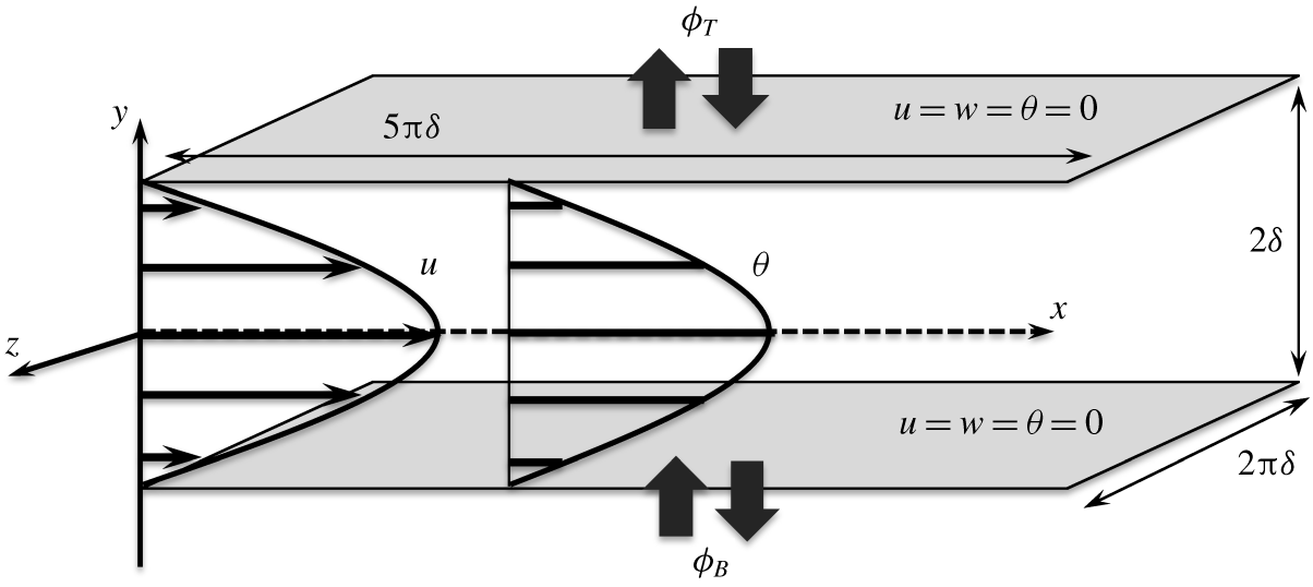
Schematic of the flow domain.

2 Numerical methods and conditions
2.1 Governing equations
We consider a fully developed turbulent flow between two parallel plates. The schematic of the computational domain and the Cartesian coordinate system are shown in figure 1. The streamwise, wall-normal and spanwise directions are denoted by ( $x_{1}$,
 $x_{2}$,
 $x_{3}$)
 $=$ (
 $x$,
 $y$,
 $z$), respectively, whereas the origin is located at the channel centre. The corresponding velocity components are denoted by (
 $u_{1}$,
 $u_{2}$,
 $u_{3}$)
 $=$ (
 $u$,
 $v$,
 $w$). In the present study, we assume the fluid is incompressible, and the effects of buoyancy are negligible. In addition, any changes in the physical and thermal properties of the fluid due to a temperature change are neglected. Consequently, the governing equations for the velocity and thermal fields are the following Navier–Stokes, continuity and passive scalar transport equations:
 $$\begin{eqnarray}\displaystyle & \displaystyle \frac{\unicode[STIX]{x2202}u_{i}}{\unicode[STIX]{x2202}t}+\frac{\unicode[STIX]{x2202}\left(u_{j}u_{i}\right)}{\unicode[STIX]{x2202}x_{j}}=-\frac{\unicode[STIX]{x2202}p}{\unicode[STIX]{x2202}x_{i}}+\frac{1}{Re}\frac{\unicode[STIX]{x2202}^{2}u_{i}}{\unicode[STIX]{x2202}x_{j}\unicode[STIX]{x2202}x_{j}}, & \displaystyle\end{eqnarray}$$
 $$\begin{eqnarray}\displaystyle & \displaystyle \frac{\unicode[STIX]{x2202}u_{i}}{\unicode[STIX]{x2202}x_{i}}=0, & \displaystyle\end{eqnarray}$$
 $$\begin{eqnarray}\displaystyle & \displaystyle \frac{\unicode[STIX]{x2202}\unicode[STIX]{x1D703}}{\unicode[STIX]{x2202}t}+\frac{\unicode[STIX]{x2202}\left(u_{j}\unicode[STIX]{x1D703}\right)}{\unicode[STIX]{x2202}x_{j}}=\frac{1}{RePr}\frac{\unicode[STIX]{x2202}^{2}\unicode[STIX]{x1D703}}{\unicode[STIX]{x2202}x_{j}\unicode[STIX]{x2202}x_{j}}+Q, & \displaystyle\end{eqnarray}$$
where  $p$ and
 $\unicode[STIX]{x1D703}$ denote static pressure and temperature, respectively. A heat source is expressed by
 $Q$, which is generally an arbitrary function of space and time. The above equations are non-dimensionalized by the bulk mean velocity
 $U_{b}^{\ast }$, the bulk mean temperature
 $\unicode[STIX]{x1D703}_{b}^{\ast }$ and the channel half-height
 $\unicode[STIX]{x1D6FF}^{\ast }$, where a quantity with an asterisk represents a dimensional value. The bulk velocity and temperature,
 $U_{b}^{\ast }$ and
 $\unicode[STIX]{x1D703}_{b}^{\ast }$, are both defined based on their volume average as follows:
 $$\begin{eqnarray}\displaystyle & \displaystyle U_{b}^{\ast }=\frac{1}{2\unicode[STIX]{x1D6FF}^{\ast }}\int _{-\unicode[STIX]{x1D6FF}^{\ast }}^{\unicode[STIX]{x1D6FF}^{\ast }}\overline{u^{\ast }}\,\text{d}y, & \displaystyle\end{eqnarray}$$
 $$\begin{eqnarray}\displaystyle & \displaystyle \unicode[STIX]{x1D703}_{b}^{\ast }=\frac{1}{2\unicode[STIX]{x1D6FF}^{\ast }}\int _{-\unicode[STIX]{x1D6FF}^{\ast }}^{\unicode[STIX]{x1D6FF}^{\ast }}\overline{\unicode[STIX]{x1D703}^{\ast }}\,\text{d}y. & \displaystyle\end{eqnarray}$$
The over-bar in (2.4) and (2.5) represents averaging over homogeneous directions  $x$ and
 $z$, and time
 $t$. We note that the above definition of
 $\unicode[STIX]{x1D703}_{b}^{\ast }$ is different from the so-called mixing-cup temperature, which is defined based on the total enthalpy flux across a cross-section. The advantage of the current definition (2.5) is that it has similar form to (2.4), so that they have exactly the same value when the velocity and temperature profiles are similar. It is known that the current definition of
 $\unicode[STIX]{x1D703}_{b}^{\ast }$ slightly overestimates the increase rate of heat transfer due to control by approximately 5 % (Hasegawa & Kasagi Reference Hasegawa and Kasagi2011). As will be shown in § 3, the heat transfer is enhanced by approximately two times compared to the uncontrolled value for the optimal input, so that the effect of the different definitions of
 $\unicode[STIX]{x1D703}_{b}^{\ast }$ remains minor, and does not change the present conclusions. The bulk Reynolds number
 $Re$ and the Prandtl number
 $Pr$ are respectively defined as
 $Re=U_{b}^{\ast }\unicode[STIX]{x1D6FF}^{\ast }/\unicode[STIX]{x1D708}^{\ast }$ and
 $Pr=\unicode[STIX]{x1D708}^{\ast }/\unicode[STIX]{x1D6FC}^{\ast }$. Here,
 $\unicode[STIX]{x1D708}^{\ast }$ represents the kinematic viscosity and
 $\unicode[STIX]{x1D6FC}^{\ast }$ is the thermal diffusivity of the fluid.
Following Hasegawa & Kasagi (Reference Hasegawa and Kasagi2011) and Yamamoto et al. (Reference Yamamoto, Hasegawa and Kasagi2013), the governing equations and boundary conditions for streamwise velocity,  $u$, and temperature,
 $\unicode[STIX]{x1D703}$, are made similar by introducing the following ideal conditions: first, the heat source term
 $Q$ is assumed to be uniform in space and is set equal to the mean pressure gradient driving the flow. Namely,
 $$\begin{eqnarray}Q=-\frac{\unicode[STIX]{x2202}\overline{p}}{\unicode[STIX]{x2202}x}.\end{eqnarray}$$
Second,  $Pr$ is set to be unity. Third,
 $u=\unicode[STIX]{x1D703}=0$ is imposed on the two walls, so that the boundary conditions for
 $u$ and
 $\unicode[STIX]{x1D703}$ are also similar. A no-slip condition is also employed for the spanwise velocity component
 $w$ on the wall, while only the wall-normal velocity component on the wall is changed in time and space in order to realize a streamwise travelling wave as explained in § 2.3.
We note that the current configuration is considered to be the most difficult case to achieve dissimilarity, while it provides a unique opportunity to discuss the effect of the continuity constraint on dissimilarity between heat and momentum transfer, since all the other sources of dissimilarity are removed. All simulations in this study are conducted under a constant flow rate condition with  $Re=U_{b}^{\ast }\unicode[STIX]{x1D6FF}^{\ast }/\unicode[STIX]{x1D708}^{\ast }=2293$, which corresponds to the friction Reynolds number of
 $Re_{\unicode[STIX]{x1D70F}}=u_{\unicode[STIX]{x1D70F}}^{\ast }\unicode[STIX]{x1D6FF}^{\ast }/\unicode[STIX]{x1D708}^{\ast }=150$ for the uncontrolled flow. Here, the friction velocity is defined as
 $u_{\unicode[STIX]{x1D70F}}^{\ast }=\sqrt{\unicode[STIX]{x1D70F}^{\ast }/\unicode[STIX]{x1D70C}^{\ast }}$, where
 $\unicode[STIX]{x1D70F}^{\ast }$ is the wall shear stress and
 $\unicode[STIX]{x1D70C}^{\ast }$ is the fluid density. Throughout the present manuscript, a quantity with the superscript of
 $+$ represents a value in the wall unit based on the friction velocity in the uncontrolled flow. In order to keep the flow rate constant, the mean pressure gradient is adjusted every time step. This means that the uniform heat source term
 $Q$ also changes in time due to (2.6). However, the temporal fluctuation of
 $-\unicode[STIX]{x2202}\overline{p}/\unicode[STIX]{x2202}x$, and thereby
 $Q$, is quite small, so that its effects on the control performances are negligible in the present configuration.
2.2 Numerical set-up
In the present DNSs, a pseudo-spectral method with Fourier expansion in the  $x$ and
 $z$ directions, and Chebyshev polynomials in
 $y$ is used for spatial discretization. The
 $3/2$-rule is applied to remove aliasing errors. The primitive variables, i.e.
 $u$,
 $v$,
 $w$ and
 $p$, are directly solved, while the pressure is decoupled from the Navier–Stokes equations (2.1) by the fractional step method (Kim & Moin Reference Kim and Moin1985). For temporal advancement, the second-order Adams–Bashforth method is applied for the convection terms, whereas the Crank–Nicolson method is used for the diffusion terms. The present code has been validated and applied to control and estimation problems of a fully developed turbulent channel flow in Hasegawa & Kasagi (Reference Hasegawa and Kasagi2011) and Suzuki & Hasegawa (Reference Suzuki and Hasegawa2017).
The dimensions of the computational domain in the streamwise, wall-normal and spanwise directions are set to be  $(L_{x},L_{y},L_{z})=(5\unicode[STIX]{x03C0},2,2\unicode[STIX]{x03C0})$. The corresponding number of modes in each direction is
 $(N_{x},N_{y},N_{z})=(128,65,128)$. The present domain widths in the
 $x$ and
 $z$ directions are twice the sizes used in Hasegawa & Kasagi (Reference Hasegawa and Kasagi2011), while the grid resolution is kept unchanged in all three directions. It has been already shown that further grid refinement does not affect the properties of the optimal control inputs obtained from the suboptimal and optimal control theories (Hasegawa & Kasagi Reference Hasegawa and Kasagi2011; Yamamoto et al. Reference Yamamoto, Hasegawa and Kasagi2013). In the present study, however, we cover a wide range of the parameter space far away from the control inputs considered in the previous studies. For this reason, we perform grid convergence studies by doubling the grid resolutions in all three directions around the globally optimal control input and also for the largest wavelength, in which the wall friction is found to be maximum. It is confirmed that the further grid refinement has minor impacts on the control performances presented in the present study. Detailed results on the grid convergence study can be found in appendix A.
All simulations start from the same initial condition, which is a fully developed state without control. The time step is set to be  $\unicode[STIX]{x0394}t^{+}=0.045$ for all cases. After starting the simulation, the magnitude of the control input is linearly increased for the initial period of
 $T^{+}=45$, and kept constant for a subsequent period of
 $T^{+}=2250$ in order to ensure that the flow reaches a fully developed state under the control. Note that a typical transient time of wall friction and wall heat flux after applying a control is found to be approximately
 $T^{+}\sim 500$ for travelling waves close to the optimal condition. After the controlled flow reaches a fully developed state, additional computation is conducted for
 $T^{+}=4500$ in order to obtain the turbulence statistics, which are presented in the following sections.
2.3 Control input
A sinusoidal travelling wave-like wall blowing and suction, which is uniform along the spanwise direction, is imposed as the control input. It can be described on the bottom wall at  $y=-1.0$ as
 $$\begin{eqnarray}v_{w}=\unicode[STIX]{x1D719}\sin \left\{\frac{2\unicode[STIX]{x03C0}}{\unicode[STIX]{x1D706}_{x}}(x-U_{p}t)\right\},\end{eqnarray}$$
where  $\unicode[STIX]{x1D719}$,
 $\unicode[STIX]{x1D706}_{x}$ and
 $U_{p}$ are the amplitude, wavelength and phase speed of the travelling wave, respectively. The subscript of
 $w$ indicates the quantity on the bottom wall. Note that the control input is applied at the two walls in a varicose mode, since it was obtained in both the suboptimal and optimal control theories (Hasegawa & Kasagi Reference Hasegawa and Kasagi2011; Yamamoto et al. Reference Yamamoto, Hasegawa and Kasagi2013). Hence, the wall-normal velocity component at the top wall (
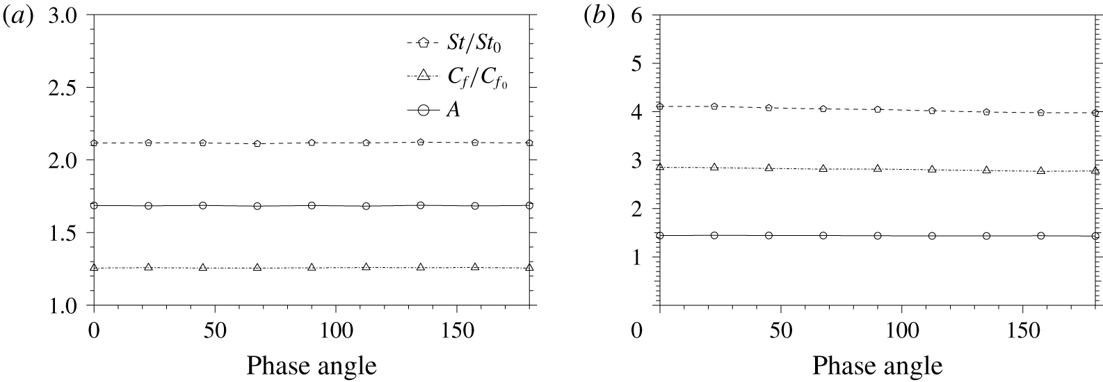
 $y=1.0$) is given by the same formula (2.7), but with the opposite sign. Although we focus on a varicose mode, the effects of the phase angle between the control inputs at the top and bottom walls are also investigated for several cases including at the global optimal point identified in the present study. We confirmed that the phase angle hardly affects the resultant control performance (see appendix B for more detailed results). The root-mean-square (r.m.s.) value of the control input is set to be 5 % of the bulk mean velocity, which is equivalent to that obtained from the optimal control theory by Yamamoto et al. (Reference Yamamoto, Hasegawa and Kasagi2013). It corresponds to the control input amplitude of
 $\unicode[STIX]{x1D719}=0.07$ or
 $\unicode[STIX]{x1D719}^{+}=1.08$ in wall units. We also note that this amplitude is smaller than that considered in Higashi et al. (Reference Higashi, Mamori and Fukagata2011), where
 $\unicode[STIX]{x1D719}^{+}$ is approximately
 $3.0$. The range of the streamwise wavelength and the phase speed considered in the present study are
 $5\unicode[STIX]{x03C0}/32\leqslant \unicode[STIX]{x1D706}_{x}\leqslant 5\unicode[STIX]{x03C0}$ and
 $-3.0\leqslant U_{p}\leqslant 3.0$, respectively. This corresponds to
 $70\lesssim \unicode[STIX]{x1D706}_{x}^{+}\lesssim 2300$ and
 $-45\lesssim U_{p}^{+}\lesssim 45$ in wall units of the uncontrolled flow. A total of 104 simulations are first conducted to cover the above mentioned parameter range, and then an additional
 $36$ cases are performed to identify the globally optimal set of the control parameters, so that the total number of simulations is 104 + 36 = 140. The largest wavelength of
 $\unicode[STIX]{x1D706}_{x}=5\unicode[STIX]{x03C0}$ considered in the study is equal to the streamwise dimension of the computational domain. Hence, we also carried out additional computations for
 $\unicode[STIX]{x1D706}=5\unicode[STIX]{x03C0}$ at different phase speeds with doubled streamwise domain size in order to confirm that the streamwise domain size does not affect the control performances.
2.4 Control performance indices
In order to quantify the control performance, three non-dimensional parameters are introduced. Namely, the skin-friction coefficient  $C_{f}$ for drag, the Stanton number
 $St$ for heat transfer and the analogy factor
 $A$ for the dissimilarity between momentum and heat transfer.
The skin-friction coefficient  $C_{f}$ is the dimensionless wall shear stress defined as
 $$\begin{eqnarray}C_{f}=\frac{\unicode[STIX]{x1D70F}^{\ast }}{\unicode[STIX]{x1D70C}^{\ast }{U_{b}^{\ast }}^{2}/2}=\frac{2}{Re}\left(\frac{\text{d}\overline{u}}{\text{d}y}\right)_{w}.\end{eqnarray}$$
By using the wall shear stress  $\unicode[STIX]{x1D70F}^{\ast }$, the pumping power per unit area required to drive the flow is calculated as,
 $P_{p}^{\ast }=U_{b}^{\ast }\unicode[STIX]{x1D70F}^{\ast }=U_{b}^{\ast }(-\text{d}\overline{p^{\ast }}/\text{d}x^{\ast })\unicode[STIX]{x1D6FF}^{\ast }$. In the uncontrolled case, the power consumption is solely determined by the pumping power
 $P_{p}^{\ast }$. In the controlled case, however, the power required to apply the control input
 $\unicode[STIX]{x1D6F1}^{\ast }$ should also be taken into account. Considering that the present control input is in a varicose mode, the controlled flow becomes statistically symmetric about the channel centre. Therefore, the following discussions only consider the bottom half of the channel without any loss of generality. The control power input at the bottom wall (
 $y=-1.0$) is given by
 $$\begin{eqnarray}\unicode[STIX]{x1D6F1}^{\ast }=\overline{\left(p_{w}^{\ast }v_{w}^{\ast }+{\textstyle \frac{1}{2}}{v_{w}^{\ast }}^{3}\right)},\end{eqnarray}$$
where the first term is the pressure work, whereas the second term corresponds to the energy flux due to the kinetic energy of the control input  $v_{w}^{\ast }$. The net power consumption (Hasegawa & Kasagi Reference Hasegawa and Kasagi2011; Yamamoto et al. Reference Yamamoto, Hasegawa and Kasagi2013) per unit wetted area is therefore introduced as
 $$\begin{eqnarray}P_{net}^{\ast }=P_{p}^{\ast }+\unicode[STIX]{x1D6F1}^{\ast }=U_{b}^{\ast }\left(-\frac{\text{d}\overline{p^{\ast }}}{\text{d}x^{\ast }}\right)\unicode[STIX]{x1D6FF}^{\ast }+\overline{\left(p_{w}^{\ast }v_{w}^{\ast }+\frac{1}{2}{v_{w}^{\ast }}^{3}\right)},\end{eqnarray}$$
where the first and second terms represent the pumping and control power inputs, respectively. The effective wall shear stress based on the net power consumption is given by
 $$\begin{eqnarray}\unicode[STIX]{x1D70F}_{net}^{\ast }=\frac{P_{net}^{\ast }}{U_{b}^{\ast }}=\left(-\frac{\text{d}\overline{p^{\ast }}}{\text{d}x^{\ast }}\right)\unicode[STIX]{x1D6FF}^{\ast }+\frac{1}{U_{b}^{\ast }}\overline{\left(p_{w}^{\ast }v_{w}^{\ast }+\frac{1}{2}{v_{w}^{\ast }}^{3}\right)},\end{eqnarray}$$
so that the corresponding skin-friction coefficient is defined as
 $$\begin{eqnarray}{C_{f}}_{net}=\frac{\unicode[STIX]{x1D70F}_{net}^{\ast }}{\unicode[STIX]{x1D70C}^{\ast }{U_{b}^{\ast }}^{2}/2}.\end{eqnarray}$$
Although  $\unicode[STIX]{x1D70F}_{net}^{\ast }$ includes the net power consumption for control, the right-hand side of (2.9) can be negative locally, indicating that an actuator receives work from the flow field. Since energy recovery through the actuator is unrealistic, a conservative definition for
 $\unicode[STIX]{x1D6F1}^{\ast }$, where negative work by actuators is not allowed, is introduced as follows:
 $$\begin{eqnarray}\unicode[STIX]{x1D6F1}_{csv}^{\ast }=\overline{\left(S_{1}p_{w}^{\ast }v_{w}^{\ast }+{\textstyle \frac{1}{2}}S_{2}{v_{w}^{\ast }}^{3}\right)}.\end{eqnarray}$$
Here, the variables  $S_{1}$ and
 $S_{2}$ are switching functions so that they become null when the control power consumption is negative locally in space and time,
 $$\begin{eqnarray}S_{1}=\left\{\begin{array}{@{}l@{}}1\quad (p_{w}^{\ast }v_{w}^{\ast }>0)\\ 0\quad (p_{w}^{\ast }v_{w}^{\ast }\leqslant 0),\end{array}\right.\quad S_{2}=\left\{\begin{array}{@{}l@{}}1\quad (v_{w}^{\ast }>0)\\ 0\quad (v_{w}^{\ast }\leqslant 0).\end{array}\right.\end{eqnarray}$$
Accordingly, the effective wall shear stress based on  $P_{csv}^{\ast }$, where
 $P_{csv}^{\ast }=P_{p}^{\ast }+\unicode[STIX]{x1D6F1}_{csv}^{\ast }$ is defined as
 $\unicode[STIX]{x1D70F}_{csv}^{\ast }=P_{csv}^{\ast }/U_{b}^{\ast }$, and the corresponding skin-friction coefficient is given by
 $$\begin{eqnarray}{C_{f}}_{csv}=\frac{\unicode[STIX]{x1D70F}_{csv}^{\ast }}{\unicode[STIX]{x1D70C}^{\ast }{U_{b}^{\ast }}^{2}/2}.\end{eqnarray}$$
As for the performance index for heat transfer, the Stanton number  $St$ is defined as
 $$\begin{eqnarray}St=\frac{q_{w}^{\ast }}{\unicode[STIX]{x1D70C}^{\ast }C_{p}^{\ast }U_{b}^{\ast }\unicode[STIX]{x1D6E9}_{b}^{\ast }}=\frac{1}{RePr}\left(\frac{\text{d}\overline{\unicode[STIX]{x1D703}}}{\text{d}y}\right)_{w},\end{eqnarray}$$
where  $q_{w}^{\ast }$ and
 $C_{p}^{\ast }$ are the heat flux at the wall and the heat capacity of the fluid, respectively.
In order to quantify dissimilarity between the momentum and heat transfer, the analogy factor  $A$ is defined as
 $$\begin{eqnarray}A\equiv \frac{2St}{C_{f}}=\left(\frac{\text{d}\overline{\unicode[STIX]{x1D703}}}{\text{d}y}\right)_{w}\left(\frac{\text{d}\overline{u}}{\text{d}y}\right)_{w}^{-1}.\end{eqnarray}$$
It is evident that  $A$ becomes unity when
 $\overline{\unicode[STIX]{x1D703}}$ and
 $\overline{u}$ have a similar profile. Such a situation can be considered as the case where the Reynold’s analogy holds perfectly. Indeed, it is almost unity for the present uncontrolled case, namely,
 $A_{0}=2St_{0}/C_{f_{0}}\approx 1.0$, where
 $C_{f_{0}}=8.58\times 10^{-3}$ and
 $St_{0}=4.30\times 10^{-3}$. Hereafter, the subscript of
 $0$ indicates a value in the uncontrolled flow. In summary, our aim is to increase
 $2St$ relative to
 $C_{f}$ so that
 $A$ becomes larger than unity. We also note that, for
 $Pr=1$ considered in the present study,
 $A/2$ is identical to
 $j/f$ which has been widely used for evaluating different heat transfer surfaces in the community of heat exchanger design, where
 $j$ and
 $f$ are the Colburn
 $j$ factor and the friction factor, respectively. In analogy to the definition of
 $A$, we can define
 $A_{net}$ and
 $A_{csv}$ based on
 ${C_{f}}_{net}$ and
 ${C_{f}}_{csv}$ as follows:
 $$\begin{eqnarray}\displaystyle & \displaystyle A_{net}=\frac{2St}{{C_{f}}_{net}}, & \displaystyle\end{eqnarray}$$
 $$\begin{eqnarray}\displaystyle & \displaystyle A_{csv}=\frac{2St}{{C_{f}}_{csv}}. & \displaystyle\end{eqnarray}$$
In the above definitions, the energy consumption for applying control is taken into account through  ${C_{f}}_{net}$ and
 ${C_{f}}_{csv}$, so that they are more suitable to evaluate the control performance from an energetic perspective.
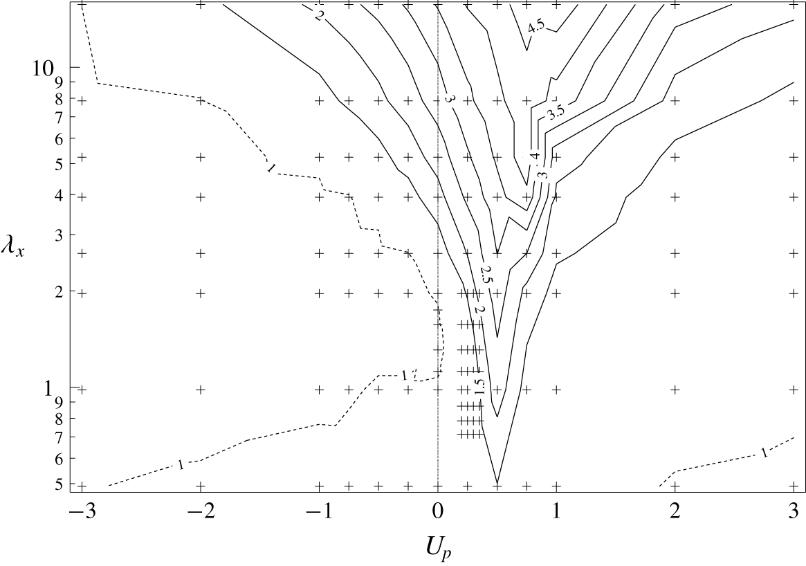
Normalized skin-friction coefficient  $C_{f}/C_{f_{0}}$. Contours with a value less than or equal to one are shown by dashed lines.

3 Control performances
3.1 Skin-friction coefficient
The skin-friction coefficient normalized by its uncontrolled value  $C_{f_{0}}$ is plotted as a function of
 $U_{p}$ and
 $\unicode[STIX]{x1D706}_{x}$ in figure 2. All the combinations of
 $\unicode[STIX]{x1D706}_{x}$ and
 $U_{p}$ for which DNSs are conducted are denoted by crosses. The contours with a value less than or equal to one are shown using dashed lines, and this applies to all the contour plots in the following sections. It is found that drag reduction is confirmed in a large area of
 $U_{p}<0$ (UTW), while prominent increase of drag is observed for
 $U_{p}>0$ (DTW), especially for
 $0<U_{p}<1$, and then the drag gradually reduces again with further increase in
 $U_{p}$ above one. The drag reduction observed for
 $U_{p}<0$ can be mostly attributed to the streaming effect (Hoepffner & Fukagata Reference Hoepffner and Fukagata2009), which drives the flow in the opposite direction to that of the applied travelling wave. For a steady wave, i.e.
 $U_{p}=0$, drag reduction is also obtained in the limited range of
 $1.12<\unicode[STIX]{x1D706}_{x}<1.74$ with a maximum drag reduction of 2 % at
 $\unicode[STIX]{x1D706}_{x}=1.30$. These results agree well with the previous findings by Quadrio, Floryan & Luchini (Reference Quadrio, Floryan and Luchini2007), where drag reduction is obtained for a turbulent channel flow at
 $Re_{\unicode[STIX]{x1D70F}}=180$ by a steady sinuous mode wave for
 $0.55<\unicode[STIX]{x1D706}_{x}<1.94$ with amplitude
 $\unicode[STIX]{x1D719}^{+}=0.70$. According to their prediction, a varicose mode with
 $\unicode[STIX]{x1D706}_{x}=1.25$ and
 $\unicode[STIX]{x1D719}^{+}=1.0$ would have resulted in a drag reduction of 2.20 % approximately (see table 1 in their appendix).
Figure 2 shows that, for any particular value of  $\unicode[STIX]{x1D706}_{x}$, the maximum value of
 $C_{f}$ occurs around
 $U_{p}$
 ${\approx}$ 0.50, and it is in agreement with the results of Mamori et al. (Reference Mamori, Iwamoto and Murata2014). This sudden increase in the value of
 $C_{f}$ around
 $U_{p}$
 ${\approx}$ 0.50 is attributed to the presence of a critical layer (Hoepffner & Fukagata Reference Hoepffner and Fukagata2009; Mamori et al. Reference Mamori, Fukagata and Hoepffner2010), which amplifies velocity fluctuations through the interaction between the mean velocity field and the control input (Maslowe Reference Maslowe1986). Similar drag increase is also reported for a streamwise travelling wave of spanwise wall forcing at both internal and external surfaces (Quadrio, Ricco & Viotti Reference Quadrio, Ricco and Viotti2009; Zhao, Huang & Xu Reference Zhao, Huang and Xu2019). In these studies, the maximum of
 $C_{f}$ occurs around
 $U_{p}^{+}=10$, which is slightly higher than that obtained in the current study. This difference would be attributed to the difference in the direction of wall forcing.
It can be seen from figure 2 that DTW also leads to drag reduction, but is limited to a quite small region of  $U_{p}>2.0$ and small
 $\unicode[STIX]{x1D706}_{x}$. Mamori et al. (Reference Mamori, Iwamoto and Murata2014) reported that even relaminarization would happen when
 $\unicode[STIX]{x1D719}^{+}>5$,
 $U_{p}^{+}>75$, and
 $200<\unicode[STIX]{x1D706}_{x}^{+}<500$. Since we consider a smaller magnitude for the control input
 $\unicode[STIX]{x1D719}^{+}=1.08$, we do not observe relaminarization, although the present ranges of
 $\unicode[STIX]{x1D706}_{x}$ and
 $U_{p}$ are similar to those considered in Mamori et al. (Reference Mamori, Iwamoto and Murata2014).
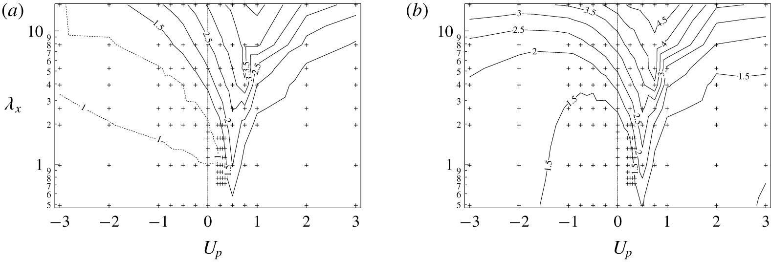
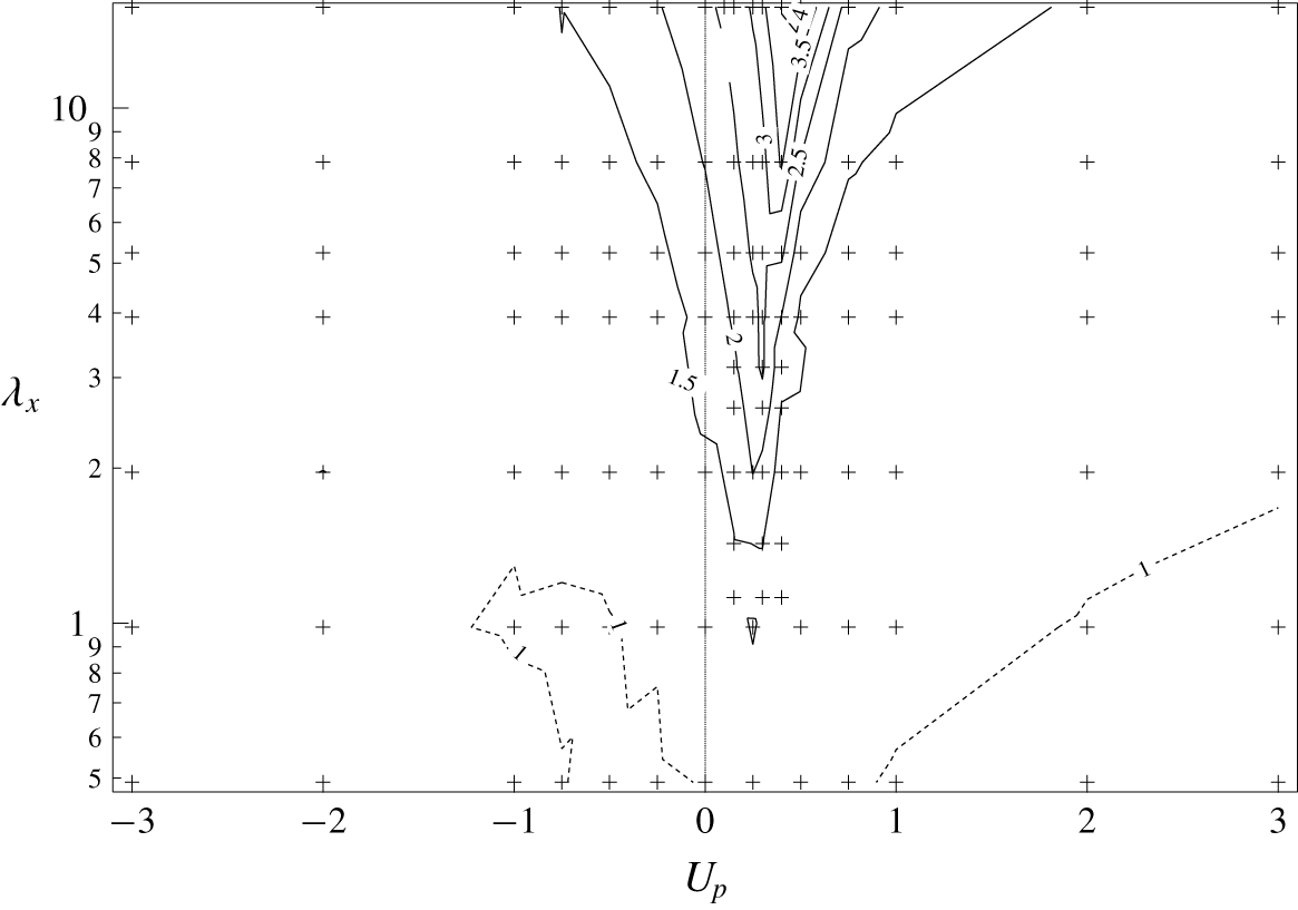
The plots of  ${C_{f}}_{net}$ and
 ${C_{f}}_{csv}$ normalized by their uncontrolled values are shown in figures 3(a) and 3(b), respectively. In accordance with their respective definitions (2.12), (2.15),
 ${C_{f}}_{net}$ can be either greater or smaller than
 $C_{f}$ depending on the sign of the net energy expenditure for control, whereas
 ${C_{f}}_{csv}$ will be always larger than
 $C_{f}$. After taking into account the power consumption for the control, the net energy saving is achieved only in a narrower region for
 ${C_{f}}_{net}$, and no energy saving is obtained in terms of
 ${C_{f}}_{csv}$ for all the cases considered presently. The above results indicate that, in the present configuration, a net energy saving is not achieved via a streamwise travelling wave of wall blowing and suction, unless the energy recovery from the flow field through actuators is allowed.
Skin-friction coefficient: (a)  ${C_{f}}_{net}/C_{f_{0}}$ and (b)
 ${C_{f}}_{csv}/C_{f_{0}}$. Contours with a value less than or equal to one are shown by dashed lines.

3.2 Stanton number
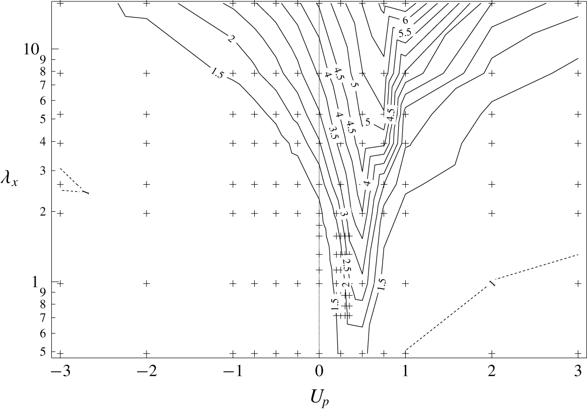
The Stanton number normalized by its uncontrolled value  $St_{0}$ is plotted as a function of
 $U_{p}$ and
 $\unicode[STIX]{x1D706}_{x}$ in figure 4. In general, the trend of
 $St/St_{0}$ is quite similar to that of
 $C_{f}/C_{f_{0}}$ shown in figure 2. However, there are two main differences. First, heat transfer enhancement is obtained for a wide region of UTW (
 $U_{p}<0$), where drag reduction is widely confirmed as shown in figure 2. Second, a similar peak of
 $St/St_{0}$ is found around
 $U_{p}$
 ${\approx}$ 0.50, while its value is larger than
 $C_{f}/C_{f_{0}}$. We also note that, unlike the contour plot of
 $C_{f}/C_{f_{0}}$, the region where heat transfer is reduced from the uncontrolled value is quite limited. This suggests that dissimilar heat transfer is achieved in a wide range of the parameter space.
Normalized Stanton number  $St/St_{0}$. Contours with a value less than or equal to one are shown by dashed lines.

3.3 Analogy factor
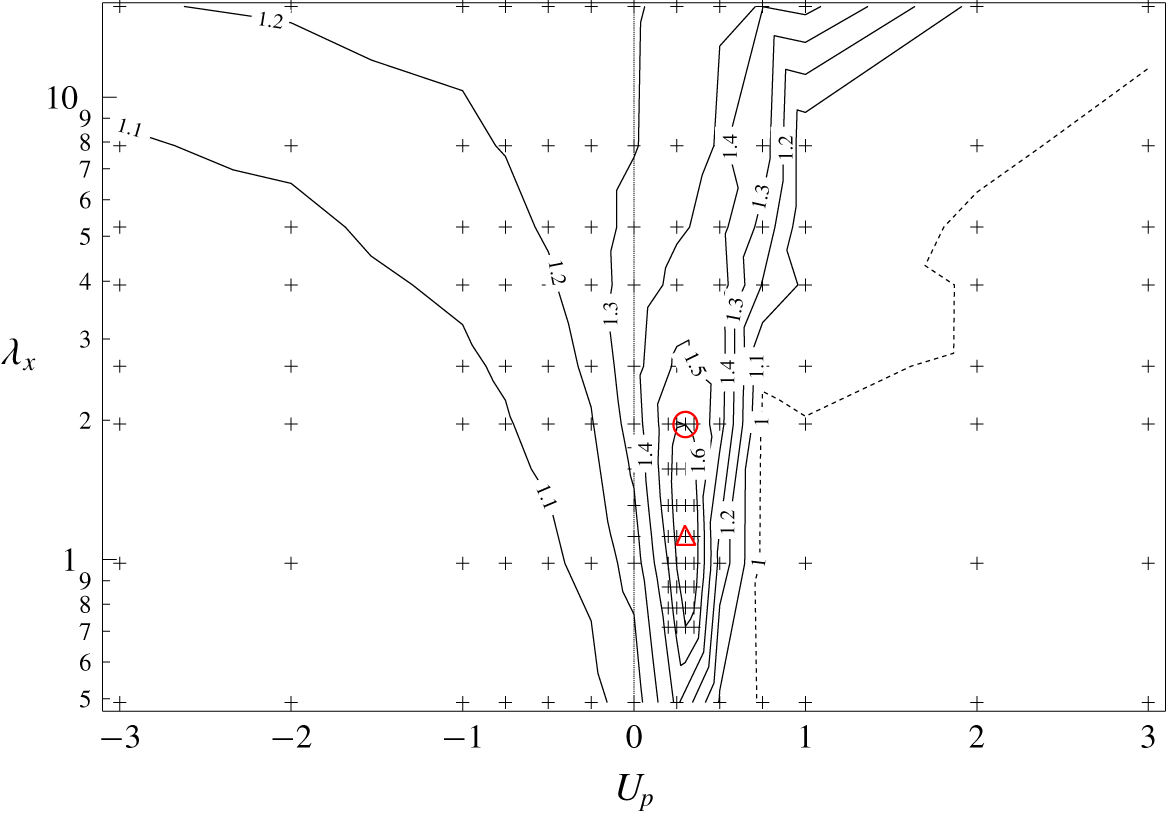
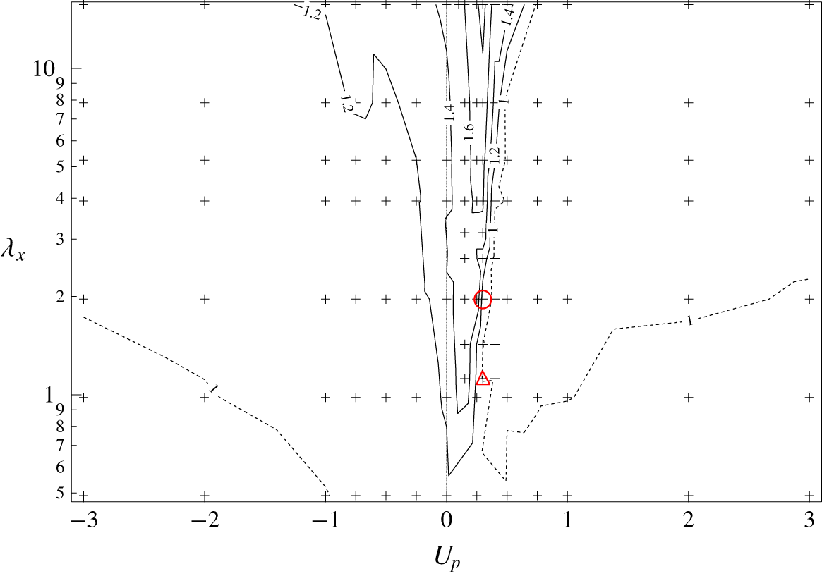
The isocontours of  $A$ are plotted as a function of
 $U_{p}$ and
 $\unicode[STIX]{x1D706}_{x}$ in figure 5. It is found that UTW achieves dissimilar control, i.e.
 $A>1$, for the entire parameter set of
 $(\unicode[STIX]{x1D706}_{x},U_{p})$ considered in the present study. This confirms the findings of Higashi et al. (Reference Higashi, Mamori and Fukagata2011), in which they obtained dissimilar heat transfer enhancement using UTW for a turbulent channel flow at
 $Re_{\unicode[STIX]{x1D70F}}\approx 180$.
Analogy factor  $A$. The red circle indicates the wave parameters
 $(\unicode[STIX]{x1D706}_{x},U_{p})=(1.96,0.30)$ obtained from the optimal control theory (Yamamoto et al. Reference Yamamoto, Hasegawa and Kasagi2013) and the red triangle indicates the global optimum of the wave parameters, i.e.
 $(\unicode[STIX]{x1D706}_{x},U_{p})=(1.12,0.30)$ obtained from the present DNSs. Contours with a value less than or equal to one are shown by dashed lines.

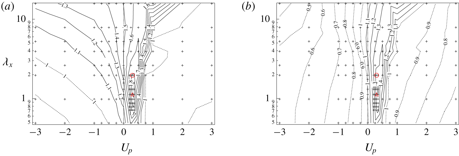
Analogy factor: (a)  $A_{net}$ and (b)
 $A_{csv}$. The circle indicates the wave parameters
 $(\unicode[STIX]{x1D706}_{x},U_{p})=(1.96,0.30)$ obtained from the optimal control theory (Yamamoto et al. Reference Yamamoto, Hasegawa and Kasagi2013) and the triangle indicates the global optimum of wave parameters
 $(\unicode[STIX]{x1D706}_{x},U_{p})=(1.12,0.30)$ obtained from the present DNSs. Contours with a value less than or equal to one are shown by dashed lines.

In contrast, more significant enhancement of  $A$ is obtained for DTW with
 $0\,<\,U_{p}<\,1$. Specifically, the maximum value of the analogy factor,
 $A=1.69$, is obtained at
 $(\unicode[STIX]{x1D706}_{x},U_{p})=(1.12,0.30)$. Hereafter, we regard this control input as the global optimum in order to distinguish it from those obtained under the suboptimal and optimal control theories. Interestingly, these optimal wave parameters are quite close to
 $(\unicode[STIX]{x1D706}_{x},U_{p})=(1.96,0.30)$ obtained via the optimal control theory by Yamamoto et al. (Reference Yamamoto, Hasegawa and Kasagi2013), where
 $A=1.55$ is achieved. Specifically, the optimal phase speed obtained from the present parametric study and that from the optimal control theory (Yamamoto et al. Reference Yamamoto, Hasegawa and Kasagi2013) are identical. The slight difference in the wavelength between the present global optimum and that obtained by the optimal control theory could be attributed to the limitation of the time horizon. In fact, in the case of the suboptimal control, where the time horizon is assumed to be vanishingly small, the wavelength of the resultant control input extends to the entire computational domain (Hasegawa & Kasagi Reference Hasegawa and Kasagi2011). Hence, there exists a trend that the wavelength obtained by the optimal control theory tends to decrease with increasing the time horizon. Considering that the present parametric survey seeks the optimum for a sufficiently large time horizon, it is consistent that the globally optimal wavelength is slightly shorter than that obtained from the optimal control theory.
The contour plots of  $A_{net}$ and
 $A_{csv}$ are presented in figure 6. Both figures clearly show that dissimilar control can be achieved even after taking into account the power required to apply the control. It is found that
 $A_{net}$ and
 $A_{csv}$ have their maximum values of 1.84 and 1.51 respectively at the same wave parameters of
 $(\unicode[STIX]{x1D706}_{x},U_{p})=(1.309,0.35)$. The global optimum of (
 $\unicode[STIX]{x1D706}_{x},U_{p}$) for
 $A_{net}$ and
 $A_{csv}$ are still close to those of
 $A$. This could be attributed to the fact that we consider a relatively small amplitude of the control input, so that the power consumption for control remains minor. The summary of control performances for the globally optimal control input is given in table 1. It should be noted that the maximum value of
 $A_{net}$ is greater than that of
 $A$, since the net control power input
 $\unicode[STIX]{x1D6F1}$ becomes negative around the optimal condition. This suggests that actuators could work without external power input ideally, or the dissimilar control could be achieved by passive means such as a properly designed compliant surface which reacts to the fluid force and induces a travelling wave close to the globally optimal mode.
Summary of the control performances for the globally optimal control input with  $(\unicode[STIX]{x1D706}_{x},U_{p})=(1.12,0.30)$.

Computational domain size, number of spectral modes, number of grid points and grid spacing in physical space and the time step used for  $Re_{\unicode[STIX]{x1D70F}}=150$ and 300, respectively.

Even after excluding the energy recovery from the actuators, dissimilar heat transfer is still confirmed with the area of  $A_{csv}>1$ shown in figure 6(b). Compared with
 $A$ shown in figure 5, however,
 $A_{csv}$ is significantly suppressed, especially for UTW. In the present configuration, there are a few cases where simultaneous drag reduction and heat transfer enhancement is achieved. Among them, a relatively large
 $A$ is achieved for
 $1.12\leqslant \unicode[STIX]{x1D706}_{x}\leqslant 1.75$ and
 $U_{p}=0$ at
 $Re_{\unicode[STIX]{x1D70F}}=150$. In these cases, however, the drag reduction rate achieved is less than 2 %, and
 $St$ is enhanced by only approximately 30 %, so that the resultant
 $A$ is limited to around 1.3 at most. In addition,
 ${C_{f}}_{csv}/{C_{f}}_{0}$ is always larger than unity, so that the UTWs are not advantageous from an energetic viewpoint. In summary, figure 3(b) together with figure 6(b) reveal that, from the energetic point of view, UTW is no longer effective for either drag reduction or dissimilar control under the small amplitude of the control input considered in the present study.
3.4 Reynolds number effect and the scaling of the optimal wave parameters
Even though it is outside the scope of the present work to extensively investigate the Reynolds number effect on the optimal travelling wave parameters, we also conduct a parametric study at  $Re=5055$, which corresponds to
 $Re_{\unicode[STIX]{x1D70F}}=300$ in the uncontrolled flow. The computational domain size, the numbers of spectral modes, the number of grid points in the physical space and the grid spacing used are outlined in table 2. The uncontrolled values of the skin-friction coefficient and the Stanton number for
 $Re_{\unicode[STIX]{x1D70F}}=300$ are
 $C_{f_{0}}=7.03\times 10^{-3}$ and
 $St_{0}=3.57\times 10^{-3}$, respectively. The magnitude of the control input with respect to the bulk mean velocity is set to be
 $\unicode[STIX]{x1D719}_{rms}=0.05$, which is the same as the cases for
 $Re_{\unicode[STIX]{x1D70F}}=150$.
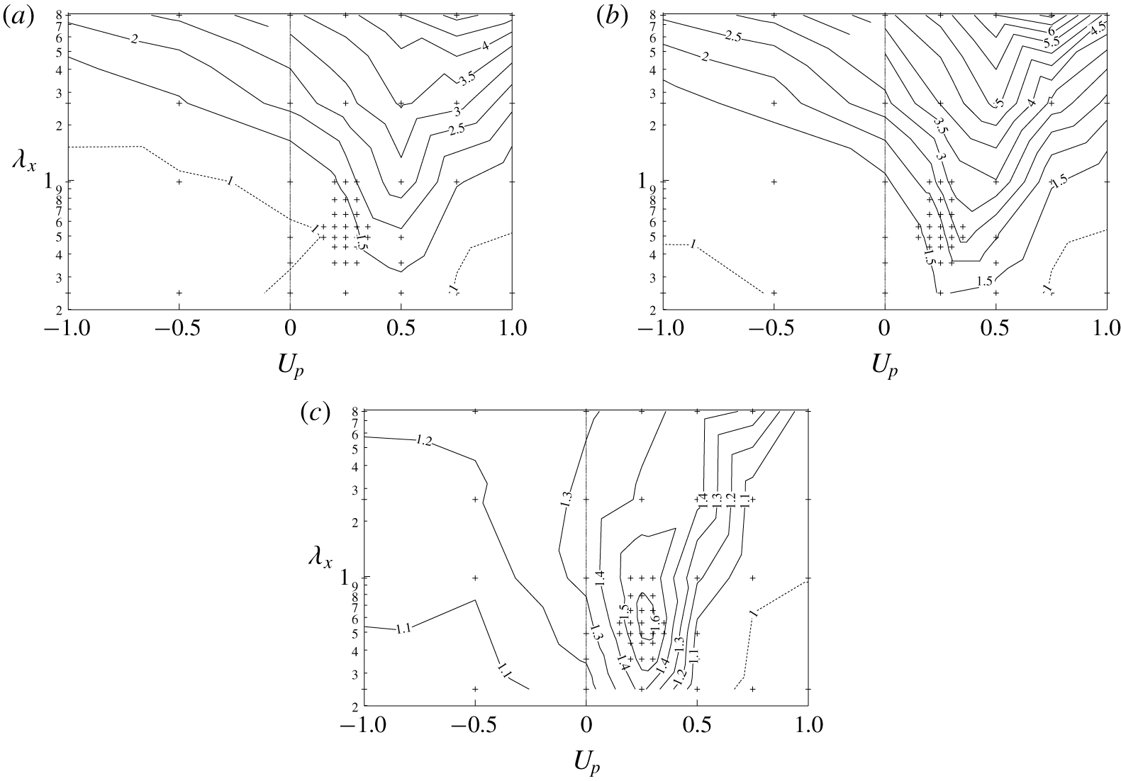
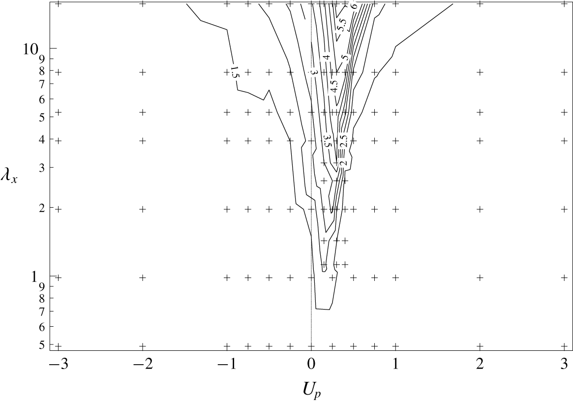
Contour plots of (a)  $C_{f}/C_{f_{0}}$, (b)
 $St/St_{0}$ and (c)
 $A$, as a function of
 $(\unicode[STIX]{x1D706}_{x},U_{p})$ for
 $Re_{\unicode[STIX]{x1D70F}}=300$. Contours with a value less than or equal to one are shown by dashed lines.

Summary of the control performances for  $Re_{\unicode[STIX]{x1D70F}}=150$ and
 $300$ at their respective optimal points. Here
 $(\unicode[STIX]{x1D706}_{x}^{+},U_{p}^{+})$ and
 $(\unicode[STIX]{x1D706}_{x_{C}}^{+},U_{p_{C}}^{+})$ respectively represent quantities normalized in wall units corresponding to the uncontrolled and controlled flow.

Among the  $56$ cases,
 $A$ has the maximum value of
 $1.62$ at
 $(\unicode[STIX]{x1D706}_{x},U_{p})=(0.65,0.25)$, as shown in figure 7. Evidently, the optimal wavelength is not scaled with the channel half-height (remember that the global optimum for
 $Re_{\unicode[STIX]{x1D70F}}=150$ is
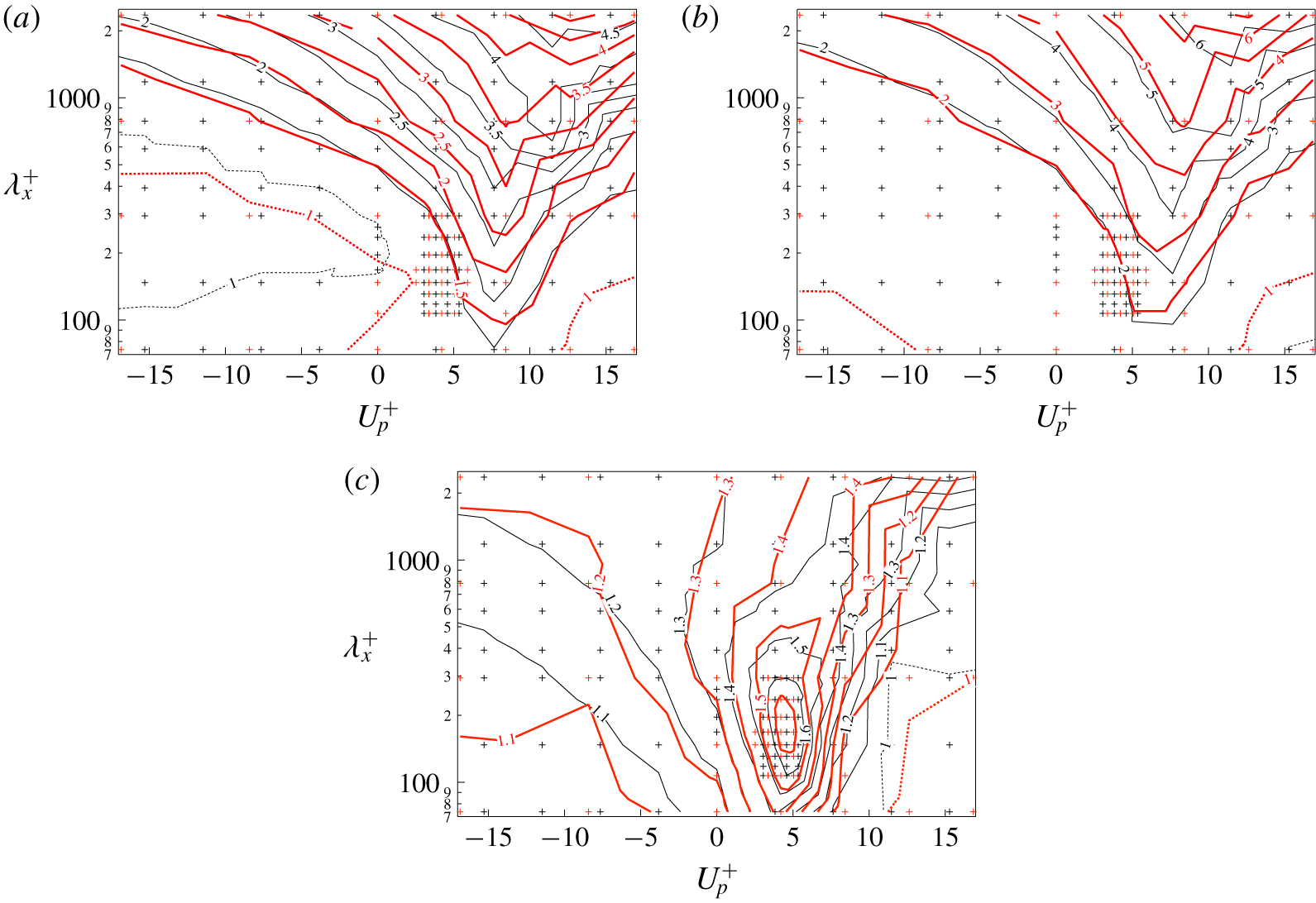
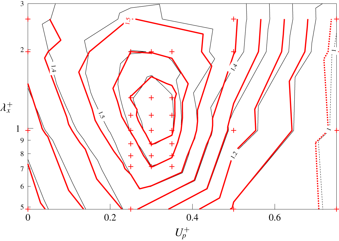
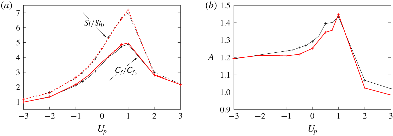
 $(\unicode[STIX]{x1D706}_{x},U_{p})=(1.12,0.3)$). Instead, the global optimum can be well scaled in the wall unit, as summarized in table 3. Figure 8 shows the contour plots of
 $C_{f}/C_{f_{0}}$,
 $St/St_{0}$ and
 $A$ as a function of
 $(\unicode[STIX]{x1D706}_{x}^{+},U_{p}^{+})$ for both
 $Re_{\unicode[STIX]{x1D70F}}=150$ (black lines) and
 $Re_{\unicode[STIX]{x1D70F}}=300$ (thick red lines). Good agreement between the respective contours of
 $Re_{\unicode[STIX]{x1D70F}}=150$ and
 $Re_{\unicode[STIX]{x1D70F}}=300$ suggests that the control performances are correlated with the wave properties in wall units. It is worth noting that an analogy factor as high as
 $1.6$ can be obtained for both
 $Re_{\unicode[STIX]{x1D70F}}=150$ and
 $Re_{\unicode[STIX]{x1D70F}}=300$ under the small amplitude of the control input considered in the present study.
So far, we have seen that DTW is particularly effective in achieving dissimilar heat transfer enhancement. In the following sections, we focus on the globally optimal travelling wave of  $(\unicode[STIX]{x1D706}_{x},U_{p})=(1.12,0.30)$ at
 $Re_{\unicode[STIX]{x1D70F}}=150$, and discuss its control mechanisms in detail by applying triple decomposition to the velocity and thermal fields and clarifying the contributions to the dissimilarity from each component.
Contour plots of (a)  $C_{f}/C_{f_{0}}$, (b)
 $St/St_{0}$ and (c)
 $A$, as a function of
 $(\unicode[STIX]{x1D706}_{x}^{+},U_{p}^{+})$ for
 $Re_{\unicode[STIX]{x1D70F}}=150$ (black lines) and
 $Re_{\unicode[STIX]{x1D70F}}=300$ (thick red lines). Contours with a value less than or equal to one are shown by dashed lines.

4 Mechanisms of dissimilarity
4.1 Triple decomposition
Since the present control applies a streamwise travelling wave of wall blowing and suction, the resultant fluctuating velocity and thermal fields can be considered as the superposition of the coherent fluctuation which travels downstream with the control input and the residual incoherent motions. Following the triple decomposition of Hussain & Reynolds (Reference Hussain and Reynolds1970), an arbitrary quantity  $f$ can be decomposed as
 $$\begin{eqnarray}f(x,y,z,t)=\langle f(\unicode[STIX]{x1D709},y)\rangle +f^{\prime \prime }(x,y,z,t),\end{eqnarray}$$
where  $\langle f\rangle$ and
 $f^{\prime \prime }$ are termed as phase-averaged and random components of
 $f$, respectively. Here,
 $\unicode[STIX]{x1D709}$, where
 $\unicode[STIX]{x1D709}=x-U_{p}t+\unicode[STIX]{x1D706}_{x}/4$, represents the streamwise coordinate that is travelling at the same speed as the control input so that
 $\unicode[STIX]{x1D709}=0$ always corresponds to the location where the wall suction becomes maximum. The phase-averaged component
 $\langle f\rangle$ can be further decomposed into mean component
 $\overline{f}$, which is an averaged quantity in the
 $x$ and
 $z$ directions and also time
 $t$, and a coherent component
 $\tilde{f}$. As a result, (4.1) can be rewritten as
 $$\begin{eqnarray}f(x,y,z,t)=\overline{f}(y)+\tilde{f}(\unicode[STIX]{x1D709},y)+f^{\prime \prime }(x,y,z,t).\end{eqnarray}$$
Consequently, the velocity and temperature fields can be decomposed into mean, coherent and random components as shown below,
 $$\begin{eqnarray}\displaystyle & \displaystyle u_{i}=\overline{u_{i}}+\tilde{u_{i}}+u_{i}^{\prime \prime }, & \displaystyle\end{eqnarray}$$
 $$\begin{eqnarray}\displaystyle & \displaystyle \unicode[STIX]{x1D703}=\overline{\unicode[STIX]{x1D703}}+\tilde{\unicode[STIX]{x1D703}}+\unicode[STIX]{x1D703}^{\prime \prime }. & \displaystyle\end{eqnarray}$$


4.2 Decomposition into coherent and random contributions
4.2.1 FIK identity
The FIK identity (Fukagata et al. Reference Fukagata, Iwamoto and Kasagi2002) is useful to distinguish between the laminar and turbulent contributions to  $C_{f}$, and can be written under a constant flow rate as
 $$\begin{eqnarray}\displaystyle {C_{f}}^{FIK}=\frac{6}{Re}+3\int _{-1}^{1}y\overline{u^{\prime }v^{\prime }}\,\text{d}y. & & \displaystyle\end{eqnarray}$$
Here, the two terms on the right-hand side quantify the contributions from the laminar and turbulent components, respectively. Similarly,  $St$ can be decomposed as (Hasegawa & Kasagi Reference Hasegawa and Kasagi2011)
 $$\begin{eqnarray}\displaystyle 2St^{FIK}=\frac{6}{Re}+3\int _{-1}^{1}y\overline{\unicode[STIX]{x1D703}^{\prime }v^{\prime }}\,\text{d}y. & & \displaystyle\end{eqnarray}$$
Since the first terms in (4.5) and (4.6) are identical and constant, the dissimilarity between  $C_{f}$ and
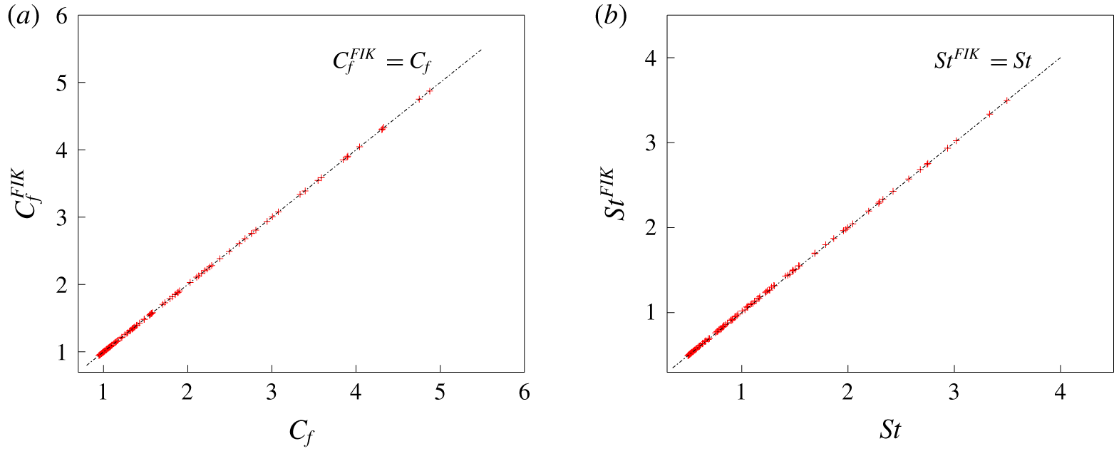
 $St$ should result from the difference between the turbulence contributions appearing as the second terms on the right-hand sides of (4.5) and (4.6). In figures 9(a) and 9(b), the values of
 $C_{f}$ and
 $St$ estimated from the FIK identity (4.5) and (4.6), i.e.
 ${C_{f}}^{FIK}$ and
 $St^{FIK}$, are compared with those obtained from direct integration of wall shear stress and wall heat flux as given by (2.8) and (2.16) for all the cases considered. It is evident that all the points fall in close proximity of the diagonal line for both
 $C_{f}$ and
 $St$. More specifically, the discrepancy between the values obtained from the two approaches is typically of the order of 0.1 % for
 $C_{f}$, while it is slightly larger (approximately 0.5 %) for
 $St$. Excellent agreement in figures 9(a) and 9(b) confirms that all the controlled flows have already reached fully developed states, and the present integration time is sufficient. Hereafter, the superscript of FIK will be omitted, since the discrepancy between
 $C_{f}$ and
 $C_{f}^{FIK}$, and that between
 $St$ and
 $St^{FIK}$ are negligibly small in comparison to their changes due to the applied control (see figures 2 and 4).
4.2.2 Decomposition of turbulent contrbituion
Decomposing the turbulent fluctuations in (4.5) and (4.6) into their coherent and random components, we obtain
 $$\begin{eqnarray}\displaystyle C_{f} & = & \displaystyle \frac{6}{Re}+3\int _{-1}^{1}y\overline{\tilde{u} \tilde{v}}\,\text{d}y+3\int _{-1}^{1}y\overline{u^{\prime \prime }v^{\prime \prime }}\,\text{d}y\nonumber\\ \displaystyle & = & \displaystyle {C_{f}}^{L}+{C_{f}}^{C}+{C_{f}}^{R},\end{eqnarray}$$
 $$\begin{eqnarray}\displaystyle 2St & = & \displaystyle \frac{6}{Re}+3\int _{-1}^{1}y\overline{\tilde{\unicode[STIX]{x1D703}}\tilde{v}}\,\text{d}y+3\int _{-1}^{1}y\overline{\unicode[STIX]{x1D703}^{\prime \prime }v^{\prime \prime }}\,\text{d}y\nonumber\\ \displaystyle & = & \displaystyle St^{L}+St^{C}+St^{R}.\end{eqnarray}$$
Here, the superscripts  $L$,
 $C$ and
 $R$ represent the laminar, coherent and random contributions, respectively. In (4.7) and (4.8), the laminar contributions are identical to those appearing as the first terms in (4.5) and (4.6), while the second turbulence contribution is decomposed into coherent and random contributions. It should be noted that the coherent contributions in the uncontrolled flow are null, i.e.
 ${{C_{f}}_{0}}^{C}={St_{0}}^{C}=0$.
For ease of analyses,  $C_{f}$ and
 $St$ are normalized with their respective values for the uncontrolled flow. After dividing by
 ${C_{f}}_{0}$ and rearranging the terms, (4.7) leads to
 $$\begin{eqnarray}\displaystyle \frac{C_{f}}{{C_{f}}_{0}} & = & \displaystyle 1+\frac{{C_{f}}^{C}-{{C_{f}}_{0}}^{C}}{{C_{f}}_{0}}+\frac{{C_{f}}^{R}-{{C_{f}}_{0}}^{R}}{{C_{f}}_{0}}\nonumber\\ \displaystyle & = & \displaystyle 1+\frac{\unicode[STIX]{x0394}{C_{f}}^{C}}{{C_{f}}_{0}}+\frac{\unicode[STIX]{x0394}{C_{f}}^{R}}{{C_{f}}_{0}}.\end{eqnarray}$$
Here,  $\unicode[STIX]{x0394}{C_{f}}^{C}$ and
 $\unicode[STIX]{x0394}{C_{f}}^{R}$ represent the variations of
 ${C_{f}}^{C}$ and
 ${C_{f}}^{R}$ from the uncontrolled values. Namely,
 $\unicode[STIX]{x0394}{C_{f}}^{C}={C_{f}}^{C}-{{C_{f}}_{0}}^{C}={C_{f}}^{C}$ and
 $\unicode[STIX]{x0394}{C_{f}}^{R}={C_{f}}^{R}-{{C_{f}}_{0}}^{R}$. Similarly, (4.8) can be rewritten as
 $$\begin{eqnarray}\displaystyle \frac{St}{St_{0}} & = & \displaystyle 1+\frac{St^{C}-{St_{0}}^{C}}{St_{0}}+\frac{St^{R}-{St_{0}}^{R}}{St_{0}}\nonumber\\ \displaystyle & = & \displaystyle 1+\frac{\unicode[STIX]{x0394}St^{C}}{St_{0}}+\frac{\unicode[STIX]{x0394}St^{R}}{St_{0}},\end{eqnarray}$$
where  $\unicode[STIX]{x0394}St^{C}=St^{C}-{St_{0}}^{C}=St^{C}$ and
 $\unicode[STIX]{x0394}St^{R}=St^{R}-{St_{0}}^{R}$. The advantage of the above expressions (4.9) and (4.10) is that the distributions shown in figures 2 and 4 are expressed as the sum of the coherent and random contributions.
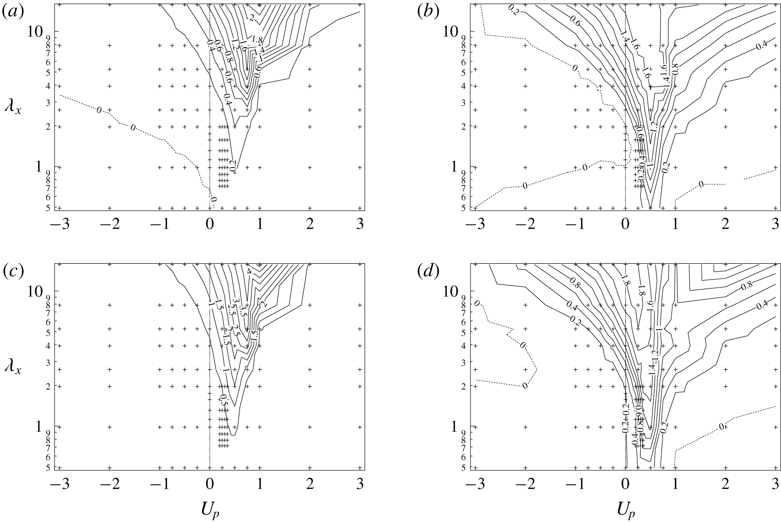
The contour plots of the four terms:  $\unicode[STIX]{x0394}{C_{f}}^{C}/{C_{f}}_{0}$,
 $\unicode[STIX]{x0394}{C_{f}}^{R}/{C_{f}}_{0}$,
 $\unicode[STIX]{x0394}St^{C}/St_{0}$ and
 $\unicode[STIX]{x0394}St^{R}/St_{0}$, are plotted as functions of
 $U_{p}$ and
 $\unicode[STIX]{x1D706}_{x}$ in figure 10. Both the coherent and random contributions have large positive values in the region of
 $0<U_{p}<1.0$, implying that a wave travelling at a similar velocity to the bulk velocity causes resonance effects, so that both contributions are enhanced. The coherent contribution to
 $C_{f}$ shown in figure 10(a) shows negative values in a wide area of
 $U_{p}<0$, whereas it is positive for
 $U_{p}>0$. This corresponds to the streaming effect, which drives a net flow in the opposite direction to the travelling wave. Meanwhile, the random contribution in figure 10(b) shows relatively small negative values for both upstream and downstream travelling waves. The suppression of the random contribution due to downstream travelling waves can be explained by the stabilizing effect (Lieu et al. Reference Lieu, Moarref and Jovanović2010).
The coherent and random contributions to  $St/St_{0}$ shown in figures 10(c) and 10(d) have generally similar trends to the corresponding contributions of
 $C_{f}/{C_{f}}_{0}$ shown in figures 10(a) and 10(b), respectively. However, the negative regions observed in figures 10(a) and 10(b) are diminished in figures 10(c) and 10(d). Especially, the negative region of
 $\unicode[STIX]{x0394}{C_{f}}^{C}/{C_{f}}_{0}$ for
 $U_{p}\leqslant 0$ in figure 10(a) totally disappears in figure 10(c), indicating that the streaming effect, which causes drag reduction always, results in heat transfer augmentation. Meanwhile, the negative regions of
 $\unicode[STIX]{x0394}{C_{f}}^{R}/{C_{f}}_{0}$ and
 $\unicode[STIX]{x0394}St^{R}/St_{0}$ in figures 10(b) and 10(d) are similar. This suggests that the stabilizing effect of DTW suppresses both skin-friction drag and heat transfer similarly. Finally, although the contour plots for coherent and random contributions to
 $St$ and
 $C_{f}$ are similar in the region of
 $0<U_{p}<1.0$, the two contributions to
 $St$ are generally larger than those to
 $C_{f}$, and this causes large dissimilarity, as will be shown in the next subsection.
Contour plots of (a)  $\unicode[STIX]{x0394}{C_{f}}^{C}/{C_{f}}_{0}$, (b)
 $\unicode[STIX]{x0394}{C_{f}}^{R}/{C_{f}}_{0}$, (c)
 $\unicode[STIX]{x0394}St^{C}/St_{0}$ and (d)
 $\unicode[STIX]{x0394}St^{R}/St_{0}$ as functions of
 $\unicode[STIX]{x1D706}_{x}$ and
 $U_{p}$. Contours with a value less than or equal to
 $0$ are shown using dashed lines.

4.2.3 Dissimilarity
In order to quantify the contributions of the coherent and random components to the dissimilarity, we introduce the following quantity  $D$ by subtracting (4.7) from (4.8):
 $$\begin{eqnarray}\displaystyle D\equiv 2St-C_{f} & = & \displaystyle 3\int _{-1}^{1}y\overline{\tilde{v}(\tilde{\unicode[STIX]{x1D703}}-\tilde{u} )}\,\text{d}y+3\int _{-1}^{1}y\overline{v^{\prime \prime }(\unicode[STIX]{x1D703}^{\prime \prime }-u^{\prime \prime })}\,\text{d}y\nonumber\\ \displaystyle & = & \displaystyle D^{C}+D^{R}.\end{eqnarray}$$
Accordingly, the analogy factor  $A$ is related to
 $D$ as follows
 $$\begin{eqnarray}\displaystyle A & = & \displaystyle 1+\frac{D}{C_{f}}\nonumber\\ \displaystyle & = & \displaystyle 1+\frac{D^{C}}{C_{f}}+\frac{D^{R}}{C_{f}},\end{eqnarray}$$
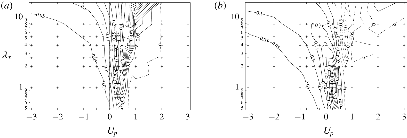
where  $D^{C}/C_{f}$ and
 $D^{R}/C_{f}$ represent the contributions of the coherent and random components to the dissimilarity, and are shown in figures 11(a) and 11(b), respectively. From figure 11(a), it can be confirmed that the coherent contribution becomes large for
 $0<U_{p}<1.0$ and increases with increasing
 $\unicode[STIX]{x1D706}_{x}$. In contrast, the random contribution shown in figure 11(b) has a positive peak at
 $(\unicode[STIX]{x1D706}_{x},U_{p})=(1.31,0.35)$, and this location is closer to the global optimum
 $(\unicode[STIX]{x1D706}_{x},U_{p})=(1.12,0.30)$ for
 $A$ shown in figure 5.
Contributions of (a) coherent and (b) random components to the analogy factor. Contours with a value less than or equal to  $0$ are shown using dashed lines.

At the globally optimal condition for  $A$, i.e.
 $(\unicode[STIX]{x1D706}_{x},U_{p})=(1.12,0.30)$, the coherent contribution
 $D^{C}$ accounts only for 38 % of the total dissimilarity
 $D$, whereas the remaining 62 % comes from the random component
 $D^{R}$. This is surprising considering the fact that the present control directly induces the coherent fluctuation, whereas the random fluctuation feels the control input only though the interaction with the induced coherent fluctuation. The present results indicate that such indirect effects on the random component cause significant dissimilarity.
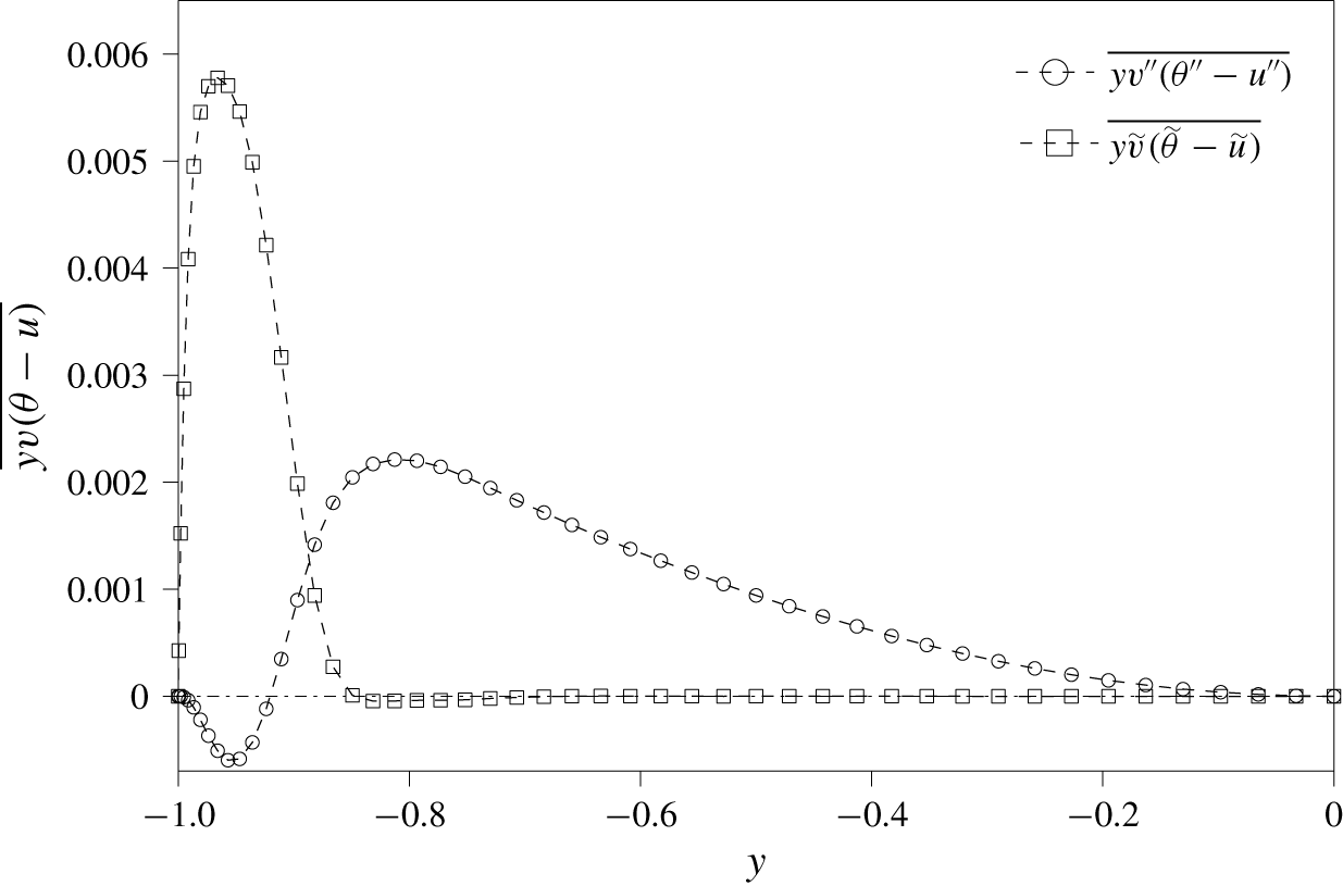
To understand the mechanism of dissimilarity in detail, we focus on the global optimal combination of  $(\unicode[STIX]{x1D706}_{x},U_{p})=(1.12,0.30)$ for further analyses. As the first step, the integrands in (4.11), i.e.
 $y\overline{\tilde{v}(\tilde{\unicode[STIX]{x1D703}}-\tilde{u} )}$ and
 $y\overline{v^{\prime \prime }(\unicode[STIX]{x1D703}^{\prime \prime }-u^{\prime \prime })}$, are plotted as a function of
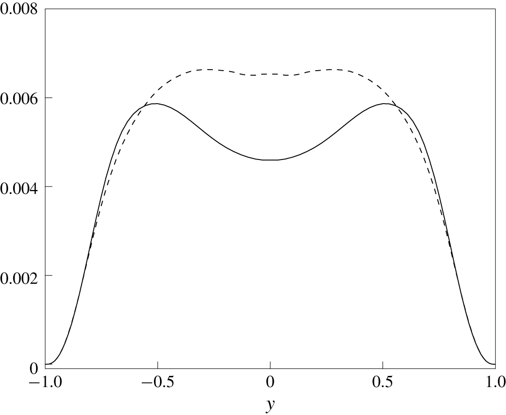
 $y$ for the lower half of the channel in figure 12. The coherent component has a positive contribution only for
 $|y|\gtrsim 0.80$. This means that the direct influence of the control input is confined to a region close to the wall. On the other hand, the random component has a negative contribution near the wall (
 $|y|\gtrsim 0.90$) and a positive contribution away from the wall
 $|y|\lesssim 0.90$. In the following sections, we discuss the origins of the coherent and random contributions in more detail.
Wall-normal distributions of the integrands of the coherent and random contributions (4.11) to dissimilarity.

4.3 Coherent contribution for the globally optimal control input
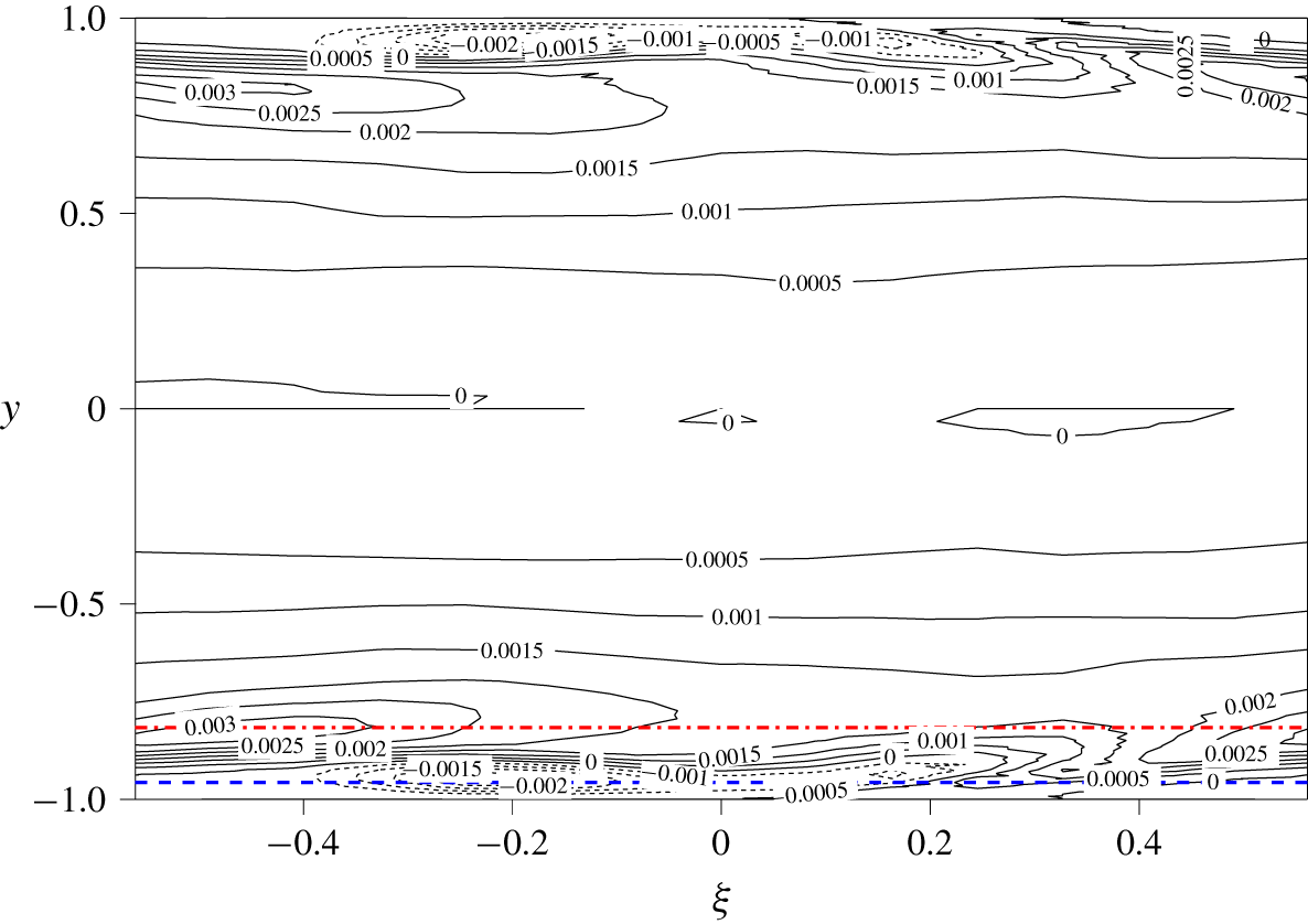
The two-dimensional distribution of the coherent contribution to dissimilarity, i.e.  $\langle y\tilde{v}(\tilde{\unicode[STIX]{x1D703}}-\tilde{u} )\rangle$, in the
 $\unicode[STIX]{x1D709}{-}y$ plane, is shown in figure 13. Note that integration of figure 13 in
 $\unicode[STIX]{x1D709}$ direction exactly reduces to the
 $y$-distribution of the coherent contribution, i.e.
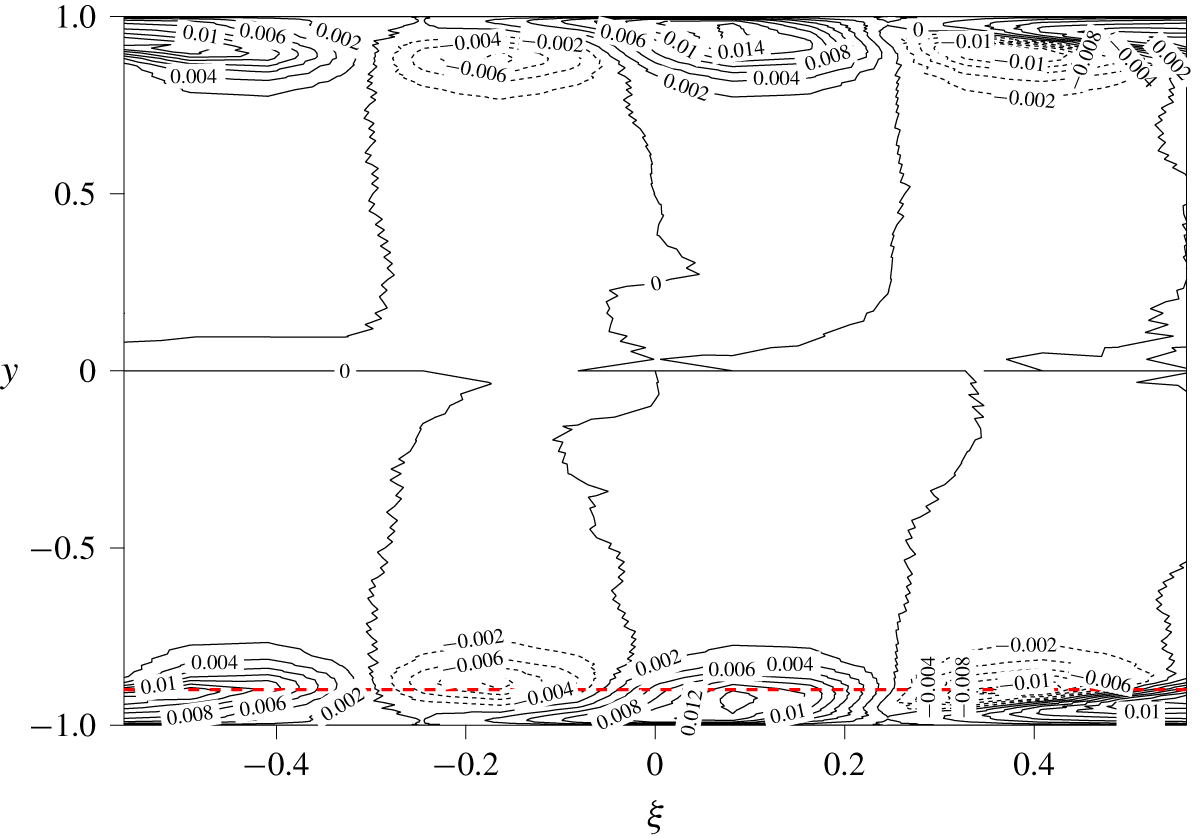
 $y\overline{\tilde{v}(\tilde{\unicode[STIX]{x1D703}}-\tilde{u} )}$, shown in figure 12. Figure 13 confirms that the coherent contribution is confined to the region close to the wall, but now its distribution in
 $\unicode[STIX]{x1D709}$ and its phase relationship with the control input can be clearly observed. A large positive contribution within
 $\unicode[STIX]{x0394}y=0.1$ from the wall (indicated by the region below the red line) is consistent with figure 12. Although large positive and negative values exist slightly away from the wall
 $(|y|<0.90)$ in figure 13, they almost cancel out each other so that their net contribution is nearly zero (see, figure 12). Closer look at the near-wall region
 $(|y|>0.9)$ reveals that the positive contours are distorted upstream, i.e. in the negative
 $\unicode[STIX]{x1D709}$ direction. We remind that the current reference frame
 $\unicode[STIX]{x1D709}-y$ is moving with the downstream travelling wave of
 $U_{p}=0.3$, and therefore the wall is moving in the negative
 $\unicode[STIX]{x1D709}$ direction in the current frame. As a result, the positive contours induced around the suction region (
 $\unicode[STIX]{x1D709}\sim 0$) is dragged below the negative contours upstream. This results in the dominant positive peak in the coherent contribution shown in figure 12.
The  $\unicode[STIX]{x1D709}{-}y$ distribution of coherent contribution
 $\langle y\tilde{v}(\tilde{\unicode[STIX]{x1D703}}-\tilde{u} )\rangle$. The red dashed line indicates the location of
 $y=-0.90$, where the coherent contribution has a positive peak. Contours with a value less than
 $0$ are shown using dashed lines.

The contour plot of the coherent components:  $\tilde{u}$,
 $\tilde{\unicode[STIX]{x1D703}}$,
 $\tilde{v}$,
 $\tilde{p}$ and (
 $\tilde{\unicode[STIX]{x1D703}}-\tilde{u}$), in the
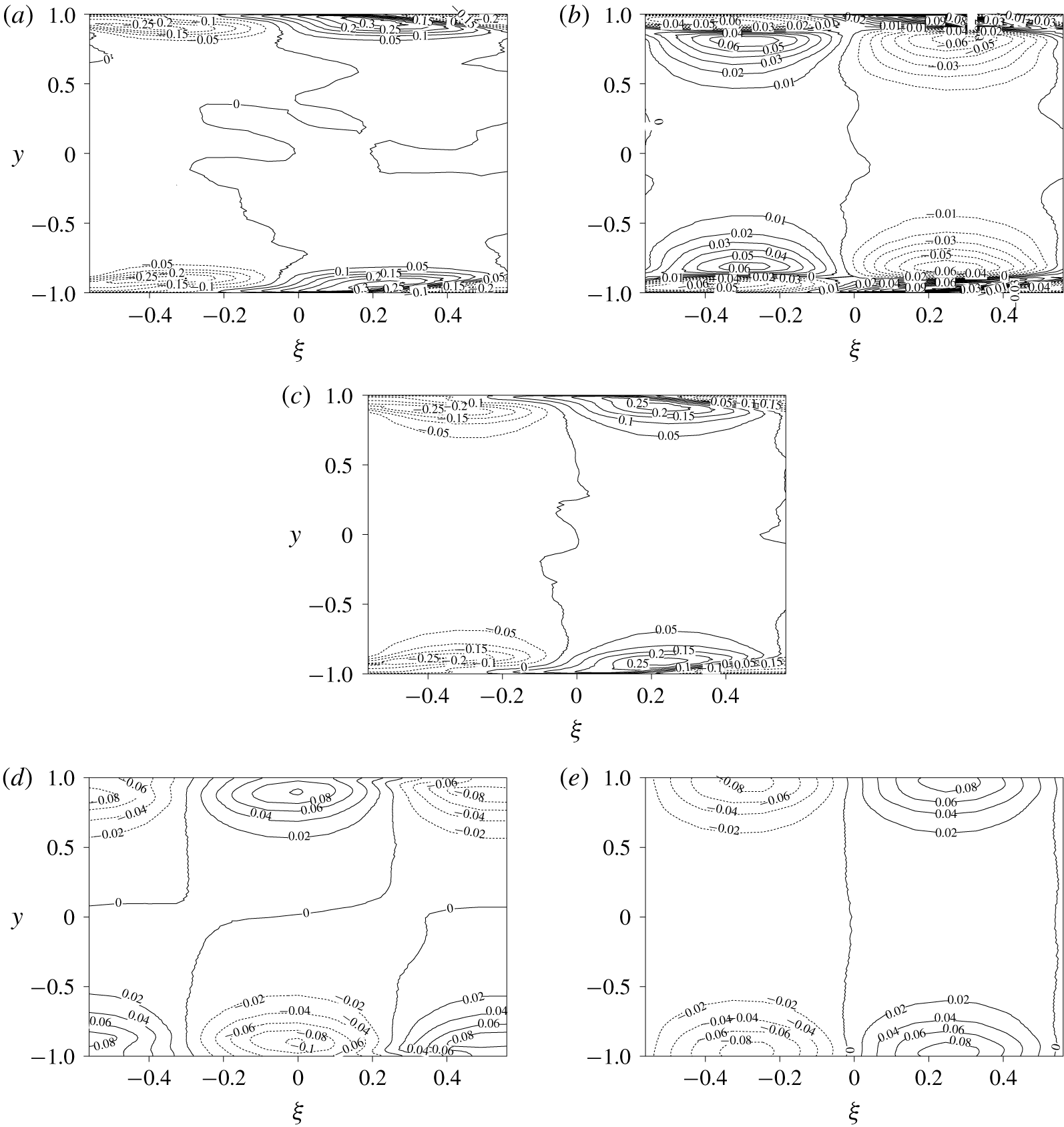
 $\unicode[STIX]{x1D709}{-}y$ plane, are plotted in figure 14. Even though the governing equations and boundary conditions are similar, the contour plots of
 $\tilde{\unicode[STIX]{x1D703}}$ and
 $\tilde{u}$ are quite different, as can be seen from figures 14(a) and 14(b). To highlight this, their difference
 $(\tilde{\unicode[STIX]{x1D703}}-\tilde{u} )$ is plotted in figure 14(c). Note that multiplying
 $(\tilde{\unicode[STIX]{x1D703}}-\tilde{u} )$ with the wall-normal coordinate
 $y$ and
 $\tilde{v}$ in figure 14(d) reproduces the contours of
 $y\tilde{v}(\tilde{\unicode[STIX]{x1D703}}-\tilde{u} )$ shown in figure 13.
Contour plots of the coherent components: (a)  $\tilde{\unicode[STIX]{x1D703}}$, (b)
 $\tilde{u}$, (c)
 $\tilde{\unicode[STIX]{x1D703}}-\tilde{u}$, (d)
 $\tilde{v}$ and (e)
 $\tilde{p}$. Contours with a value less than
 $0$ are shown using dashed lines.

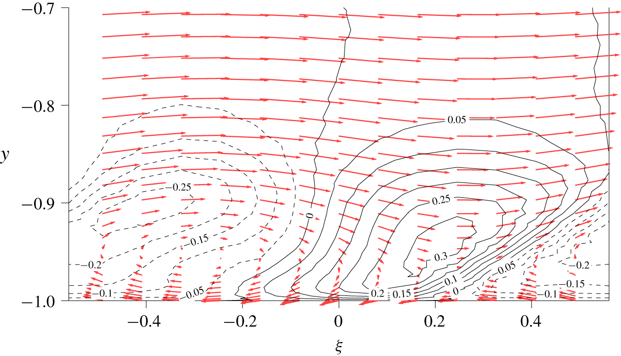
In order to explain the distribution of  $\tilde{\unicode[STIX]{x1D703}}$ shown in figure 14(a), an enlarged view of
 $\tilde{\unicode[STIX]{x1D703}}$ with phase-averaged velocity field,
 $(\langle u\rangle -U_{p},\tilde{v})$, is shown in figure 15 for the near-wall region. Since the frame is moving with the applied travelling wave, we subtract the phase speed from the phase-averaged streamwise velocity to show the relative velocity. We can identify three characteristic features in figure 15. First, in the near-wall region of
 $|y|>0.90$, the downwelling motion due to wall suction around
 $\unicode[STIX]{x1D709}=0$ brings high-temperature fluid toward the wall, resulting in positive
 $\tilde{\unicode[STIX]{x1D703}}$ contours, and the opposite happens near the blowing regions around
 $\unicode[STIX]{x1D709}=\pm 0.56$. Second, the convection outside the near-wall region,
 $|y|<0.90$ transports the temperature fluctuation
 $\tilde{\unicode[STIX]{x1D703}}$ downstream. Third, the wall movement at the speed of
 $-U_{p}$ drags
 $\tilde{\unicode[STIX]{x1D703}}$ upstream due to the viscous effect in the near-wall region of
 $|y|>0.90$.
Enlarged view of  $\tilde{\unicode[STIX]{x1D703}}$ in the near-wall region. The vectors show the phase-averaged velocity field
 $(\langle u\rangle -0.30,\tilde{v})$. Contours with a value less than
 $0$ are shown using dashed lines.

Next, we consider the contour plot of  $\tilde{u}$ shown in figure 14(b). Although
 $\tilde{u}$ is similar to
 $\tilde{\unicode[STIX]{x1D703}}$, shown in figure 14(a) in the vicinity of the wall, it shows large fluctuations with the opposite sign away from the wall. This distinct difference between
 $\tilde{\unicode[STIX]{x1D703}}$ and
 $\tilde{u}$ can be explained by the pressure gradient term present only in the governing equation for
 $\tilde{u}$ (see equations (C 4) and (C 5) in appendix C). The wall blowing around
 $\unicode[STIX]{x1D709}=\pm 0.56$ causes a favourable pressure gradient, whereas the wall suction around
 $\unicode[STIX]{x1D709}=0$ results in an adverse pressure gradient (see figure 14e). The induced coherent pressure gradient only affects the dynamics of
 $\tilde{u}$, and therefore creates significant dissimilarity between
 $\tilde{\unicode[STIX]{x1D703}}$ and
 $\tilde{u}$. The current results indicate that the coherent contribution is caused by the combined effects of the following two mechanisms. First, the continuity constraint, i.e. the pressure fluctuation, modifies only the dynamics of
 $\tilde{u}$, so that it causes the dissimilarity between
 $\tilde{\unicode[STIX]{x1D703}}$ and
 $\tilde{u}$. Second, the induced dissimilarity
 $(\tilde{\unicode[STIX]{x1D703}}-\tilde{u} )$ is dragged into the near-wall region due to fluid viscosity, and this generates the coherent contribution,
 $\langle y\tilde{v}(\tilde{\unicode[STIX]{x1D703}}-\tilde{u} )\rangle$, through interaction with
 $\tilde{v}$ induced by the control input.
The above two mechanisms become further apparent from the budget of the coherent contribution, i.e.  $-\overline{\tilde{v}(\tilde{\unicode[STIX]{x1D703}}-\tilde{u} )}$, (see (D 7) and its detailed derivation in § D.1),
 $$\begin{eqnarray}\displaystyle 0 & = & \displaystyle \underbrace{\overline{\tilde{v}^{2}}\frac{\unicode[STIX]{x2202}(\bar{\unicode[STIX]{x1D703}}-\bar{u})}{\unicode[STIX]{x2202}y}}_{P_{C}}\underbrace{-\overline{\widetilde{u_{j}^{\prime \prime }v^{\prime \prime }}\frac{\unicode[STIX]{x2202}(\tilde{\unicode[STIX]{x1D703}}-\tilde{u} )}{\unicode[STIX]{x2202}x_{j}}}}_{P_{C1_{C}}}\underbrace{-\overline{\{\widetilde{u_{j}^{\prime \prime }(\unicode[STIX]{x1D703}^{\prime \prime }-u^{\prime \prime })}\}\frac{\unicode[STIX]{x2202}\tilde{v}}{\unicode[STIX]{x2202}x_{j}}}}_{P_{C2_{C}}}\nonumber\\ \displaystyle & & \displaystyle +\,\underbrace{\frac{\unicode[STIX]{x2202}}{\unicode[STIX]{x2202}y}\overline{\left[(\tilde{\unicode[STIX]{x1D703}}-\tilde{u} )\widetilde{v^{\prime \prime }v^{\prime \prime }}+\tilde{v}\{\widetilde{v^{\prime \prime }(\unicode[STIX]{x1D703}^{\prime \prime }-u^{\prime \prime })}\}+\tilde{v}\tilde{v}(\tilde{\unicode[STIX]{x1D703}}-\tilde{u} )\right]}}_{T_{D_{C}}}\underbrace{-\frac{1}{Re}\frac{\unicode[STIX]{x2202}}{\unicode[STIX]{x2202}y}\overline{\left[\frac{\unicode[STIX]{x2202}\tilde{v}(\tilde{\unicode[STIX]{x1D703}}-\tilde{u} )}{\unicode[STIX]{x2202}y}\right]}}_{V_{D_{C}}}\nonumber\\ \displaystyle & & \displaystyle \underbrace{-\,\overline{\left\{-(\tilde{\unicode[STIX]{x1D703}}-\tilde{u} )\frac{\unicode[STIX]{x2202}\tilde{p}}{\unicode[STIX]{x2202}y}+\tilde{v}\frac{\unicode[STIX]{x2202}\tilde{p}}{\unicode[STIX]{x2202}x}\right\}}}_{\unicode[STIX]{x1D6F1}_{C}}\nonumber\\ \displaystyle & & \displaystyle \underbrace{+\,\frac{2}{Re}\overline{\frac{\unicode[STIX]{x2202}\tilde{v}}{\unicode[STIX]{x2202}x_{j}}\frac{\unicode[STIX]{x2202}(\tilde{\unicode[STIX]{x1D703}}-\tilde{u} )}{\unicode[STIX]{x2202}x_{j}}}}_{\unicode[STIX]{x1D716}_{C}}.\end{eqnarray}$$
The first three terms in the first line on the right-hand side represent the production (termed as  $P_{C}$,
 $P_{C1_{C}}$ and
 $P_{C2_{C}}$). The second line corresponds to turbulent and molecular diffusion (denoted as
 $T_{D_{C}}$ and
 $V_{D_{C}}$), whereas the third line is the correlation between velocity/temperature fluctuation and pressure gradient (
 $\unicode[STIX]{x1D6F1}_{C}$). The final term represents the molecular dissipation (
 $\unicode[STIX]{x1D716}_{C}$). Here, the subscript
 $C$ indicates the budget terms of the coherent contribution. It will be shown that the last two production terms (i.e.
 $P_{C1_{C}}$ and
 $P_{C2_{C}}$) also appear in the budget equation of the random contribution, i.e.
 $-\overline{v^{\prime \prime }(\unicode[STIX]{x1D703}^{\prime \prime }-u^{\prime \prime })}$, but with the opposite sign (see (4.14)). Therefore, they represent the exchange between the coherent and random contributions and are referred to as the coupling terms hereafter.
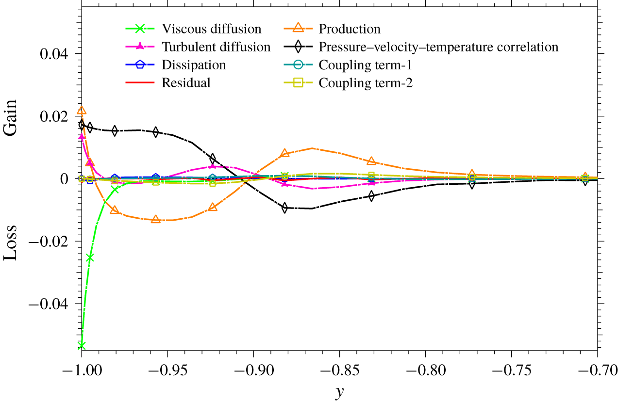
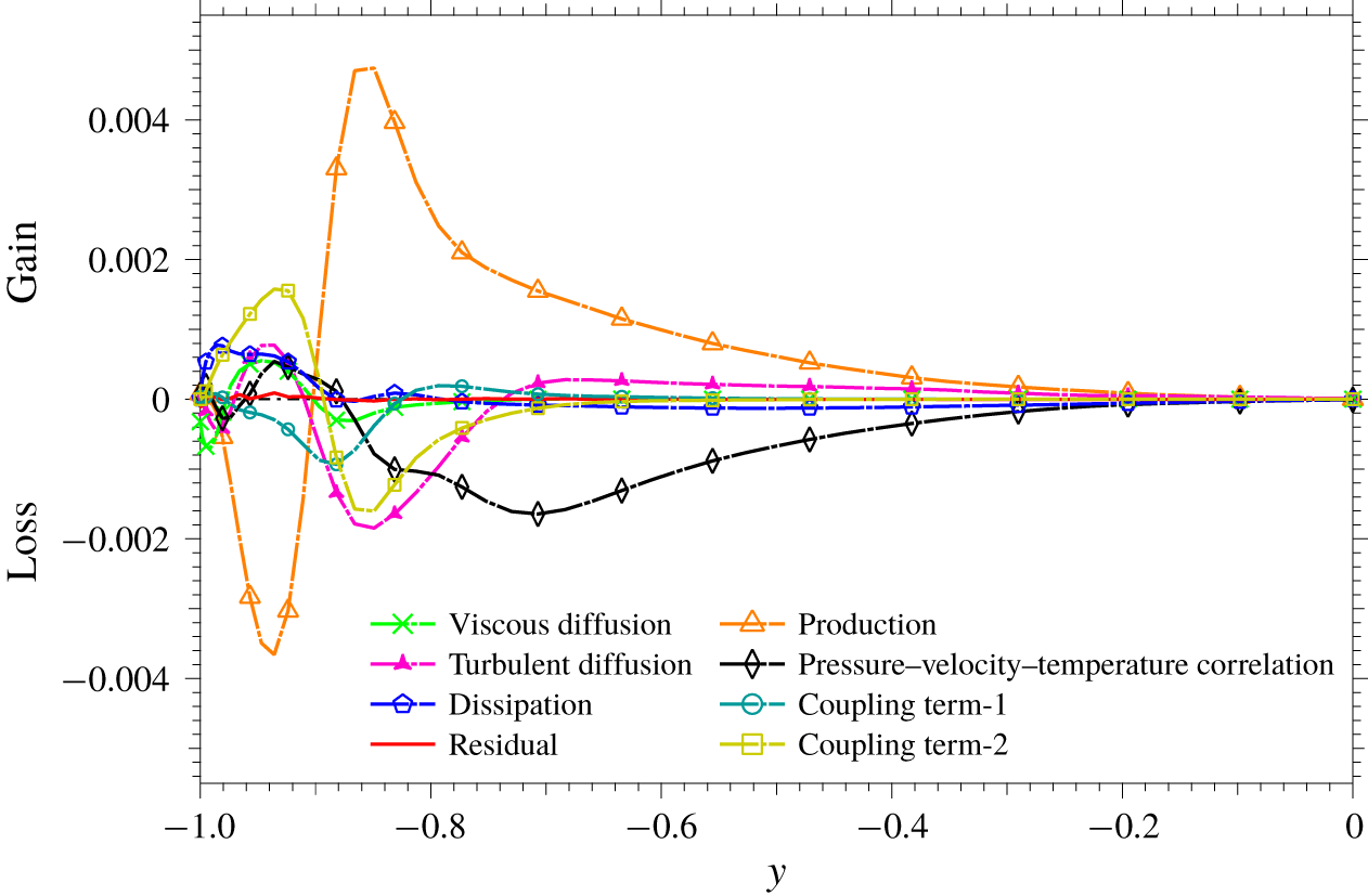
Each term in the budget equation (4.13) is plotted in figure 16. The plot indicates that  $\unicode[STIX]{x1D6F1}_{C}$ and
 $P_{C}$ act as the dominant positive and negative terms in the near-wall region,
 $-0.97<y<-0.90$, respectively. Here, we remind that the pressure fluctuation is a primary factor causing dissimilarity in the coherent field. This can be confirmed by a dominant positive value of
 $\unicode[STIX]{x1D6F1}_{C}$ in the near-wall region,
 $y<-0.90$, where the coherent contribution becomes significant (see, figure 12). Slightly away from the wall beyond
 $y=-0.90$,
 $\unicode[STIX]{x1D6F1}_{C}$ and
 $P_{C}$ are still dominant, but change their signs. Further away from the wall (
 $y\gtrsim -0.80$), all budget terms decay and this also agrees with the decay of the coherent contribution in figure 12. In the immediate vicinity from the wall, i.e.
 $y<-0.97$ (
 $y^{+}<5$), the contribution from the molecular diffusion becomes significant; in fact for
 $y^{+}<5$ the positive contributions from
 $\unicode[STIX]{x1D6F1}_{C}$,
 $P_{C}$ and
 $T_{D_{C}}$ are balanced solely by
 $V_{D_{C}}$. So, even though viscous dissipation is minor throughout the channel, viscosity plays a crucial role in the dissimilar heat transfer process very close to the wall. Finally, we note that the coupling terms, i.e.
 $P_{C1_{C}}$, and
 $P_{C2_{C}}$, are generally quite small within the entire region, suggesting that the direct interaction between the coherent and random components is relatively weak.
Terms in the budget equation for  $-\overline{\tilde{v}(\tilde{\unicode[STIX]{x1D703}}-\tilde{u} )}$:
 $P_{C}$
= production;
 $P_{C1_{C}}$ and
 $P_{C2_{C}}$
= coupling terms;
 $T_{D_{C}}$ and
 $V_{D_{C}}$
= turbulent and molecular diffusion;
 $\unicode[STIX]{x1D6F1}_{C}=$ correlation between velocity/temperature fluctuation and pressure gradient;
 $\unicode[STIX]{x1D716}_{C}=$ molecular dissipation.

4.4 Random contribution for the globally optimal control input
In figure 12, there exist two distinct peaks in the plot of random contribution to dissimilarity, i.e.  $\overline{yv^{\prime \prime }\left(\unicode[STIX]{x1D703}^{\prime \prime }-u^{\prime \prime }\right)}$, close to the wall. One positive peak at
 $y_{p}=-0.81$ (
 $y^{+}=28.08$ from the bottom wall) and one negative peak at
 $y_{n}=-0.96$ (
 $y^{+}=6.47$). In order to understand their generation mechanisms, we consider the following budget equation for
 $-\overline{v^{\prime \prime }(\unicode[STIX]{x1D703}^{\prime \prime }-u^{\prime \prime })}$ (see (D 8) and its detailed derivation in § D.2),
 $$\begin{eqnarray}\displaystyle 0= & & \displaystyle \underbrace{\overline{{v^{\prime \prime }}^{2}}\frac{\unicode[STIX]{x2202}(\bar{\unicode[STIX]{x1D703}}-\bar{u})}{\unicode[STIX]{x2202}y}}_{P_{R}}\underbrace{+\overline{\widetilde{u_{j}^{\prime \prime }v^{\prime \prime }}\frac{\unicode[STIX]{x2202}(\tilde{\unicode[STIX]{x1D703}}-\tilde{u} )}{\unicode[STIX]{x2202}x_{j}}}}_{P_{C1_{R}}}\underbrace{+\overline{\widetilde{u_{j}^{\prime \prime }(\unicode[STIX]{x1D703}^{\prime \prime }-u^{\prime \prime })}\frac{\unicode[STIX]{x2202}\tilde{v}}{\unicode[STIX]{x2202}x_{j}}}}_{P_{C2_{R}}}\nonumber\\ \displaystyle & & \displaystyle \underbrace{+\frac{\unicode[STIX]{x2202}}{\unicode[STIX]{x2202}y}\overline{\left[\tilde{v}\{\widetilde{v^{\prime \prime }(\unicode[STIX]{x1D703}^{\prime \prime }-u^{\prime \prime })}\}+v^{\prime \prime }v^{\prime \prime }(\unicode[STIX]{x1D703}^{\prime \prime }-u^{\prime \prime })\right]}}_{T_{D_{R}}}\underbrace{+\frac{1}{Re}\frac{\unicode[STIX]{x2202}}{\unicode[STIX]{x2202}y}\overline{\left[\frac{\unicode[STIX]{x2202}v^{\prime \prime }(\unicode[STIX]{x1D703}^{\prime \prime }-u^{\prime \prime })}{\unicode[STIX]{x2202}y}\right]}}_{V_{D_{R}}}\nonumber\\ \displaystyle & & \displaystyle \underbrace{-\overline{\left\{-(\unicode[STIX]{x1D703}^{\prime \prime }-u^{\prime \prime })\frac{\unicode[STIX]{x2202}p^{\prime \prime }}{\unicode[STIX]{x2202}y}+v^{\prime \prime }\frac{\unicode[STIX]{x2202}p^{\prime \prime }}{\unicode[STIX]{x2202}x}\right\}}}_{\unicode[STIX]{x1D6F1}_{R}}\nonumber\\ \displaystyle & & \displaystyle \underbrace{+\frac{2}{Re}\overline{\frac{\unicode[STIX]{x2202}v^{\prime \prime }}{\unicode[STIX]{x2202}x_{j}}\frac{\unicode[STIX]{x2202}(\unicode[STIX]{x1D703}^{\prime \prime }-u^{\prime \prime })}{\unicode[STIX]{x2202}x_{j}}}}_{\unicode[STIX]{x1D716}_{R}}.\end{eqnarray}$$
Similar to (4.13), the first three terms, i.e.  $P_{R}$,
 $P_{C1_{R}}$ and
 $P_{C2_{R}}$, in the first line on the right-hand side represent the production. The second line corresponds to turbulent and molecular diffusion (denoted as
 $T_{D_{R}}$ and
 $V_{D_{R}}$), whereas the third line is the correlation between velocity/temperature fluctuation and pressure gradient (
 $\unicode[STIX]{x1D6F1}_{R}$). The final term represents the molecular dissipation (
 $\unicode[STIX]{x1D716}_{R}$). Here, the subscript
 $R$ indicates the budget terms of the random contribution.
In figure 17, all the budget terms in (4.14) are plotted. The term  $P_{R}$ represents a source term through the interaction of the mean component with the random component, and is found to be the most dominant term. Also, their positive and negative peaks agree well with those observed in the profile of the random contribution (see figure 12). Since
 $\overline{{v^{\prime \prime }}^{2}}$ is always positive, the sign of
 $P_{R}$ is determined by the sign of
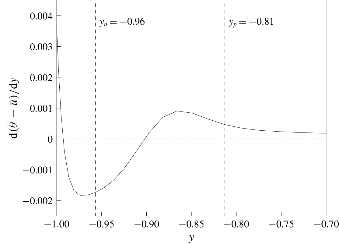
 $\text{d}(\bar{\unicode[STIX]{x1D703}}-\bar{u})/\text{d}y$. The variation of
 $\text{d}(\bar{\unicode[STIX]{x1D703}}-\bar{u})/\text{d}y$ along the lower half of the channel is plotted in figure 18. It is found that the profile of
 $\text{d}(\bar{\unicode[STIX]{x1D703}}-\bar{u})/\text{d}y$ changes its sign between the peak locations
 $y_{p}$ and
 $y_{n}$, and this explains why the sign of the random contribution changes in figure 12. It should be noted that the mechanisms of the random contribution is in contrast to those of the coherent contribution, where the correlation term between velocity/temperature and pressure gradient,
 $\unicode[STIX]{x1D6F1}_{C}$, is dominant.
As mentioned in the previous subsection, the coupling terms  $P_{C1_{R}}$ and
 $P_{C2_{R}}$ have exactly the same form as
 $P_{C1_{C}}$ and
 $P_{C2_{C}}$ in (4.13) with opposite signs, indicating that they represent direct interaction between the coherent and random contributions. In general, they make minor contributions throughout the domain, as shown in figure 17. It should be noted, however, that they have the opposite sign to
 $P_{R}$, indicating that the random contribution generated by
 $P_{R}$ is transported to the coherent contribution through
 $P_{C1_{R}}$ and
 $P_{C2_{R}}$.
Terms in the budget equation for  $-\overline{v^{\prime \prime }(\unicode[STIX]{x1D703}^{\prime \prime }-u^{\prime \prime })}$:
 $P_{R}=\text{production}$;
 $P_{C1_{R}}$ and
 $P_{C2_{R}}=\text{coupling}\,\text{terms}$;
 $T_{D_{R}}$ and
 $V_{D_{R}}=\text{turbulent}$ and molecular diffusion;
 $\unicode[STIX]{x1D6F1}_{R}=\text{correlation}$ between velocity/temperature fluctuation and pressure gradient;
 $\unicode[STIX]{x1D716}_{R}$
= molecular dissipation.

Gradient of the difference between the mean temperature and velocity along the lower half of the channel.  $y_{p}=-0.96$ and
 $y_{n}=-0.81$ correspond to the locations where the random contribution to dissimilarity has positive and negative peaks, respectively.

The  $\unicode[STIX]{x1D709}{-}y$ distribution of the random contribution
 $\langle y(\unicode[STIX]{x1D703}^{\prime \prime }v^{\prime \prime }-u^{\prime \prime }v^{\prime \prime })\rangle$. The dash-dotted line (red) and dashed (blue) line represent the location of
 $y_{p}=-0.81$ and
 $y_{n}=-0.96$ where the random contribution to dissimilarity has positive and negative peaks, respectively. Contours with a value less than
 $0$ are shown using dashed lines.

The distribution of  $\langle y(\unicode[STIX]{x1D703}^{\prime \prime }v^{\prime \prime }-u^{\prime \prime }v^{\prime \prime })\rangle$ in the
 $\unicode[STIX]{x1D709}{-}y$ plane is shown in figure 19. The integration of the plotted quantity in
 $\unicode[STIX]{x1D709}$ gives the distribution of the random contribution as a function of
 $y$ presented in figure 12. The red dash-dotted and blue dashed lines correspond to the negative and positive peaks of the random contribution, i.e.
 $y=y_{n}$ and
 $y_{p}$ near the bottom wall, respectively. Strong negative contours are confirmed around
 $y=y_{n}$, where
 $y\overline{v^{\prime \prime }(\unicode[STIX]{x1D703}^{\prime \prime }-u^{\prime \prime })}$ shown in figure 12 also has a negative peak. The negative contours are particularly concentrated around the suction region, i.e.
 $\unicode[STIX]{x1D709}\sim 0$. Meanwhile, positive contours exist slightly away from the wall above wall blowing region (
 $\unicode[STIX]{x1D709}\sim \pm 0.56$), and this location also agrees with the positive peak location of the random contribution shown in figure 12.
For further analyses of the random contribution, we express the momentum and heat transfer of the random fields with the eddy viscosity and diffusivity, i.e.  $E_{v}^{^{\prime \prime }}$ and
 $E_{d}^{^{\prime \prime }}$, which are respectively defined as
 $$\begin{eqnarray}\displaystyle & \displaystyle \langle -v^{\prime \prime }u^{\prime \prime }\rangle =E_{v}^{^{\prime \prime }}\frac{\unicode[STIX]{x2202}\langle u\rangle }{\unicode[STIX]{x2202}y}, & \displaystyle\end{eqnarray}$$
 $$\begin{eqnarray}\displaystyle & \displaystyle \langle -v^{\prime \prime }\unicode[STIX]{x1D703}^{\prime \prime }\rangle =E_{d}^{^{\prime \prime }}\frac{\unicode[STIX]{x2202}\langle \unicode[STIX]{x1D703}\rangle }{\unicode[STIX]{x2202}y}, & \displaystyle\end{eqnarray}$$
where  $E_{v}^{^{\prime \prime }}$ and
 $E_{d}^{^{\prime \prime }}$ are functions of
 $\unicode[STIX]{x1D709}$ and
 $y$. Accordingly, the random contribution can be rewritten as
 $$\begin{eqnarray}\displaystyle \langle -v^{\prime \prime }(\unicode[STIX]{x1D703}^{\prime \prime }-u^{\prime \prime })\rangle & = & \displaystyle \left(E_{d}^{^{\prime \prime }}\frac{\unicode[STIX]{x2202}\langle \unicode[STIX]{x1D703}\rangle }{\unicode[STIX]{x2202}y}-E_{v}^{^{\prime \prime }}\frac{\unicode[STIX]{x2202}\langle u\rangle }{\unicode[STIX]{x2202}y}\right),\nonumber\\ \displaystyle & = & \displaystyle E_{v}^{^{\prime \prime }}\frac{\unicode[STIX]{x2202}\langle u\rangle }{\unicode[STIX]{x2202}y}\left(\frac{E_{d}^{^{\prime \prime }}}{E_{v}^{^{\prime \prime }}}\frac{\unicode[STIX]{x2202}\langle \unicode[STIX]{x1D703}\rangle /\unicode[STIX]{x2202}y}{\unicode[STIX]{x2202}\langle u\rangle /\unicode[STIX]{x2202}y}-1\right),\nonumber\\ \displaystyle & = & \displaystyle E_{v}^{^{\prime \prime }}\frac{\unicode[STIX]{x2202}\langle u\rangle }{\unicode[STIX]{x2202}y}\left({Pr_{t}^{^{\prime \prime }}}^{-1}S-1\right),\end{eqnarray}$$
where the turbulent Prandtl number for the random field is defined as
 $$\begin{eqnarray}Pr_{t}^{^{\prime \prime }}=\frac{E_{v}^{^{\prime \prime }}}{E_{d}^{^{\prime \prime }}},\end{eqnarray}$$
and the ratio of the wall-normal gradients of the phase-averaged velocity and temperature fields is given by
 $$\begin{eqnarray}S=\frac{\text{d}\langle \unicode[STIX]{x1D703}\rangle /\text{d}y}{\text{d}\langle u\rangle /\text{d}y}.\end{eqnarray}$$
If the analogy between the velocity and thermal fields holds well, it is expected that both  $S$ and
 $Pr_{t}^{^{\prime \prime }}$ are close to unity. In such a case, equation (4.17) indicates that the random contribution should also vanish. Meanwhile, when either
 $S$ or
 $Pr_{t}^{^{\prime \prime }}$ deviates from unity, the random contribution becomes non-zero. In figures 20(a) and 20(b),
 $S$ and
 $Pr_{t}^{^{\prime \prime }-1}$ are plotted in the
 $\unicode[STIX]{x1D709}{-}y$ plane, respectively. Again, the vertical locations of
 $y_{n}$ and
 $y_{p}$ are depicted by the dash-dotted red line and the dashed blue line, respectively. From the comparison of figures 20(a) and 20(b), the concentrated negative and positive contours in figure 19 are strongly correlated with
 $S$ rather than
 $Pr_{t}^{^{\prime \prime }-1}$. Considering the definition of
 $S$ given in (4.19), the random contribution is mainly caused by the dissimilarity between the phase-averaged velocity and temperature fields. If one refers to the coherent contribution discussed in § 4.3 to the direct effect, the random contribution can be viewed as the indirect effect, since it is associated with the changes in the phase-averaged fields.
(a) The ratio of the wall-normal gradients of the phase-averaged temperature and velocity fields,  $S$, and (b) the inverse of the turbulent Prandtl number for the random component,
 $\left(Pr_{t}^{^{\prime \prime }}\right)^{-1}$. The red dash-dotted and blue dashed lines represent the locations of
 $y_{p}=-0.81$ and
 $y_{n}=-0.96$ where the random contribution to dissimilarity has positive and negative peaks, respectively. Contours with a value less than or equal to
 $1$ are shown using dashed lines.

Instantaneous distribution of the random contribution  $yv^{\prime \prime }(\unicode[STIX]{x1D703}^{\prime \prime }-u^{\prime \prime })$ in the bottom half of the channel at
 $\unicode[STIX]{x1D709}=0$. An enlarged view of the near-wall region is shown in the bottom figure. The vectors show the random velocity components
 $(v^{\prime \prime },w^{\prime \prime })$. The red dash-dotted and blue dashed lines represent the locations of
 $y_{p}=-0.81$ and
 $y_{n}=-0.96$ where the random contribution to dissimilarity has positive and negative peaks, respectively.

Top view of the isosurfaces of  $Q^{+}=-0.03$ for the uncontrolled (a) and controlled (b) (for the optimal case) channel flow at
 $Re_{\unicode[STIX]{x1D70F}}=150$.

Isosurfaces of  $Q^{+}=0.03$ (white),
 $yv^{\prime \prime }(\unicode[STIX]{x1D703}^{\prime \prime }-u^{\prime \prime })=0.01$ (red) and
 $yv^{\prime \prime }(\unicode[STIX]{x1D703}^{\prime \prime }-u^{\prime \prime })=-0.01$ (blue) for the bottom half of
 $(a)$ uncontrolled flow and
 $(b)$ controlled flow with the globally optimal input at
 $Re_{\unicode[STIX]{x1D70F}}=150$. The arrows in the controlled case represents wall blowing and suction which is uniform in the spanwise direction.

An instantaneous snapshot of the bottom half of the channel in the  $y{-}z$ plane at
 $\unicode[STIX]{x1D709}=0$ is shown in figure 21. An enlarged view of near-wall region is shown in the bottom figure. The colour represents the random contribution
 $yv^{\prime \prime }(\unicode[STIX]{x1D703}^{\prime \prime }-u^{\prime \prime })$, and the random velocity vectors are also shown with arrows. The statistical features shown so far can also be confirmed in an instantaneous field. Specifically, the random component tends to have negative values around the blue horizontal line which corresponds to the negative peak location of the random contribution shown in figure 12, whereas positive regions occur relatively away from the wall and they distribute around the red line corresponding to the positive peak location in figure 12. These negative and positive random contributions are mostly associated with either strong downwelling or upwelling motions. This is again consistent with the first production term in the budget equation (D 8) of the random contributions.
4.5 Visualization of the turbulence structures
In order to discuss the relationship between near-wall turbulent structures and the coherent and random contributions, instantaneous flow fields in the uncontrolled and controlled flows are shown in figure 22. Here, the  $Q$ criterion defined as
 $Q=-\unicode[STIX]{x2202}u_{i}/\unicode[STIX]{x2202}x_{j}\unicode[STIX]{x2202}u_{j}/\unicode[STIX]{x2202}x_{i}$ (Hunt, Wray & Moin Reference Hunt, Wray and Moin1988) is used to visualize vortex cores.
Comparison between figures 22(a) and 22(b) reveals two distinct features of the controlled flow. First, there exist spanwise rollers which is directly induced by wall blowing/suction. The spanwise rolls exist below  $y^{+}=15$, and agree well with the coherent flow field drawn by vectors in figure 15. Second, above the spanwise rollers, there exists quasi-streamwise vortices similar to those in the uncontrolled flow, but with finer length scale. As far as we observed the temporal evolution of the turbulent structures, there is no clear evidence that the coherent spanwise rolls and the quasi-streamwise interact directly. Rather, the quasi-streamwise vortices emerge and breakdown almost in a irrelevant manner to the spanwise rolls. Spanwise two-point correlations of the random velocity fluctuations
 $u^{\prime \prime }$ and
 $v^{\prime \prime }$ indicate that the spanwise distances of the negative peaks are almost unchanged when they are normalized by the wall unit based on the actual wall shear. These results suggest that the modification of near-wall turbulent structures due to the globally optimal control input is mainly caused by the change of averaged wall shear, rather than the direct interaction between the coherent and random fields. This is also consistent with the budget analyses in the previous subsections.
Quasi-streamwise vortices induce  $v^{\prime \prime }$, and therefore produce the random contribution through
 $P_{R}=\overline{{v^{\prime \prime }}^{2}}\unicode[STIX]{x2202}(\bar{\unicode[STIX]{x1D703}}-\bar{u})/\unicode[STIX]{x2202}y$ according to the budget equation (4.14) for the random contribution. In figure 23, the isosurfaces of the positive and negative random contributions are drawn in red and blue together with the isosurface of
 $Q^{+}$ shown in white. It can be confirmed that the random contributions wrap around quasi-streamwise vortices. Positive random contributions (red) are prominent away from the wall, whereas negative contributions (blue) are clustering around the legs of quasi-streamwise vortices near the wall. These results are consistent with the positive and negative peaks in the profile of the random contribution shown in figure 12 and also the two-dimensional visualization shown in figure 21.
5 Discussion
The present results indicate that the performance of dissimilar control is determined as a result of the complex responses of coherent and random fields to the travelling wave-like wall blowing and suction. Considering the complexity of the phenomena, it is rather surprising that the optimal control theory predicted the global optimal parameters of the travelling wave fairly well.
One possible reason for its success is that there exist no multiple local maxima in the analogy factor within the parameter range considered in the present study as shown in figure 5. Since the optimal control theory iteratively optimizes a control input based on the local gradient of a given cost functional, the resultant control input could be stuck in a local minimum. Hence, the presence of a single minimum/maximum is necessary for a gradient-based optimization to predict the global optimum. Nonetheless, it does not always guarantee success. As described in § 1, the optimal control theory takes into account future flow dynamics within only a limited time horizon ( $T^{+}\approx 100$), which is much smaller than a period required for a flow field to reach another equilibrium state under a certain control input. In order to fill the temporal gap, a time-division technique is commonly used. Namely, once the control input converges in a given time horizon, the time horizon is advanced in time and new optimization procedures are conducted (Bewley, Moin & Temam Reference Bewley, Moin and Temam2001; Yamamoto et al. Reference Yamamoto, Hasegawa and Kasagi2013). These processes will be repeated until multiple time horizons cover a sufficiently long period, so that the controlled flow eventually reaches a statistically equilibrium state.
A key feature of the present control input is a travelling wave-like property. When observed from a frame moving with the applied control input, the resultant phase-averaged velocity and thermal fields become steady, as shown in § 4. Therefore, as far as the phase-averaged velocity and thermal fields are concerned, the problem reduces to the optimization of a steady flow. In such a case, even though each time horizon is relatively short, it could be possible that the control input eventually approaches to the global optimum by sequentially repeating the optimization procedure for a long period.
Meanwhile, the coherent velocity and thermal fields are not solely determined by the control input, but also interact with the random field as can be seen in the governing equations for the coherent field (see (C 4)–(C 6)). Such nonlinear interactions are generally slow processes, so that a sufficiently long time horizon should be necessary in order to correctly take into account their effects in the optimization procedures. In addition, the present DNS results indicate that the random contribution to dissimilarity is more significant than that due to the coherent contribution. These facts suggest that predicting the globally optimal mode by the optimal control theory should be quite challenging.
According to the present results in § 4.5, however, the random contribution to dissimilar heat transfer enhancement is mostly caused by the dissimilarity between the phase-averaged velocity and thermal fields (more specifically, the ratio of their wall-normal gradients,  $S$) rather than the variation of the turbulent Prandtl number. This means that the local similarity between momentum and heat transfer still holds well even in the controlled flow, and the distributions of the phase-averaged velocity and thermal fields govern not only the coherent contribution, but also the random contribution. This could be a reason why the optimal control theory with a limited time horizon still provides a good prediction of the globally optimal travelling wave properties.
Wall-normal distributions of the eddy viscosity  $E_{v_{0}}$ (solid line) and eddy diffusivity
 $E_{d_{0}}$ (dashed line) for the uncontrolled flow.

The above discussions motivate us to propose a simple approach where only the phase-averaged velocity and thermal fields are directly solved, while the effects of the random field are represented by eddy viscosity and eddy diffusivity models. In order to demonstrate such a possibility, we consider the following equations for the phase-averaged velocity and thermal fields:
 $$\begin{eqnarray}\displaystyle & \displaystyle \frac{\unicode[STIX]{x2202}\langle u_{i}\rangle }{\unicode[STIX]{x2202}x_{i}}=0, & \displaystyle\end{eqnarray}$$
 $$\begin{eqnarray}\displaystyle & \displaystyle \frac{\unicode[STIX]{x2202}\langle u_{i}\rangle }{\unicode[STIX]{x2202}t}+\frac{\unicode[STIX]{x2202}(\langle u_{j}\rangle \langle u_{i}\rangle )}{\unicode[STIX]{x2202}x_{j}}=-\frac{\unicode[STIX]{x2202}\langle p\rangle }{\unicode[STIX]{x2202}x_{i}}+\frac{\unicode[STIX]{x2202}}{\unicode[STIX]{x2202}x_{j}}\left\{\left(\frac{1}{Re}+E_{v}^{\prime \prime }\right)\left(\frac{\unicode[STIX]{x2202}\langle u_{i}\rangle }{\unicode[STIX]{x2202}x_{j}}+\frac{\unicode[STIX]{x2202}\langle u_{j}\rangle }{\unicode[STIX]{x2202}x_{i}}\right)\right\}, & \displaystyle\end{eqnarray}$$
 $$\begin{eqnarray}\displaystyle & \displaystyle \frac{\unicode[STIX]{x2202}\langle \unicode[STIX]{x1D703}\rangle }{\unicode[STIX]{x2202}t}+\frac{\unicode[STIX]{x2202}(\langle u_{j}\rangle \langle \unicode[STIX]{x1D703}\rangle )}{\unicode[STIX]{x2202}x_{j}}=Q+\frac{\unicode[STIX]{x2202}}{\unicode[STIX]{x2202}x_{j}}\left\{\left(\frac{1}{Pe}+E_{d}^{\prime \prime }\right)\frac{\unicode[STIX]{x2202}\langle \unicode[STIX]{x1D703}\rangle }{\unicode[STIX]{x2202}x_{j}}\right\}. & \displaystyle\end{eqnarray}$$
 $E_{v}$ and
 $E_{d}$ in (5.1) are functions of space and their distributions depend on an applied control input. Meanwhile, according to the finding in the previous section, the impact of the turbulent Prandtl number on dissimilar heat transfer is relatively weak. Therefore, we assume that
 $E_{v}$ and
 $E_{d}$ are unchanged from the uncontrolled values, and only functions of
 $y$. The vertical profiles of
 $E_{v}$ and
 $E_{d}$ assumed in the present URANS are shown in figure 24. The advantage of the present approach is that the profiles of
 $E_{v}$ and
 $E_{d}$ in the uncontrolled flow are relatively easy to obtain.
Analogy factor  $A$ obtained from URANS simulations. The circle and triangle indicate the control input obtained from the optimal control theory (Yamamoto et al. Reference Yamamoto, Hasegawa and Kasagi2013) and the global optimum obtained in the present DNS, respectively. Contours with a value less than or equal to
 $1$ are shown using dashed lines.

The URANS equations are numerically solved in a two-dimensional  $\unicode[STIX]{x1D709}-y$ domain. An energy-conservative second-order central difference scheme is used for the spatial discretization and low-storage third-order Runge–Kutta/Crank–Nicolson scheme for the time integration (Kametani & Fukagata Reference Kametani and Fukagata2011). The streamwise length of the domain is changed accordingly so as to accommodate one wavelength of the control input, whereas the wall-normal length is kept constant and equal to
 $2$. The number of grid points employed in the streamwise and wall-normal directions are
 $(N_{x},Ny)=(20,96)$. The Reynolds and Péclet numbers are set to be identical to those in the present DNS, namely,
 $Re=Pe=2293$. Since the current URANS only solves the phase-averaged velocity and thermal fields in the two-dimensional domain, it is much cheaper than conducting unsteady three-dimensional DNS.
The contour plot of the analogy factor obtained from the URANS is shown in figure 25. A direct comparison with figure 5 reveals that the overall trend of the present DNS is well captured by the URANS calculation. Specifically, URANS predicts a large peak around  $U_{p}=0.3$ and this agrees well with the present DNS results. Meanwhile, in URANS, the analogy factor increases with increasing wavelength, so that no global maximum of
 $A$ is found. This trend of overestimating the wavelength is also found in the control inputs obtained from the suboptimal and optimal control theories as mentioned before. The present results suggest that inaccurate evaluation of the random contribution overestimates the wavelength of the optimal travelling wave. Although these discrepancies exist, we should rather emphasized that the present URANS succeeds in predicting the overall trend of
 $A$ despite its simplicity.
The normalized skin-friction coefficient and Stanton number obtained from the URANS are also shown in figures 26 and 27. Their strong similarity to those obtained from DNS shown in figures 2 and 4 are also confirmed. In both DNS and URANS, the values of  $C_{f}/C_{f_{0}}$ and
 $St/St_{0}$ increase with
 $\unicode[STIX]{x1D706}_{x}$. Also, for any particular value of
 $\unicode[STIX]{x1D706}_{x}$, the maximum values for
 $C_{f}/C_{f_{0}}$ and
 $St/St_{0}$ occur between
 $0<U_{p}<1.0$ where the critical layer amplifies the fluctuations. Meanwhile, the URANS commonly underestimates both
 $C_{f}/C_{f_{0}}$ and
 $St/St_{0}$, and this is mainly attributed to the fact that our current eddy viscosity and eddy diffusivity models are assumed to be kept unchanged from the uncontrolled values regardless of an applied control. Indeed, according to the DNS results, both
 $E_{v}^{\prime \prime }$ and
 $E_{d}^{\prime \prime }$ are increased when the globally optimal travelling wave is applied (not shown here). Even in such a situation, however, their ratio, i.e. the turbulent Prandtl number, does not deviate from unity significantly, so that it hardly contributes to dissimilarity as indicated by (4.17). As a result, the present URANS can still capture the overall trend of
 $A$.
Contour plot of  $C_{f}/C_{f_{0}}$ obtained from URANS. Contours with a value less than or equal to
 $1$ are shown using dashed lines.

Contour plot of  $St/St_{0}$ obtained from URANS.

6 Conclusions
We conducted a series of DNSs of a fully developed channel flow subject to travelling wave-like wall blowing and suction at the bulk Reynolds number of  $Re=2293$ in order to clarify its impact on the dissimilarity between turbulent momentum and heat transfer. While keeping the wave amplitude constant as 5 % of the bulk mean velocity, the wavelength and phase speed of the travelling wave were systematically changed in a wide parameter range, i.e.
 $5\unicode[STIX]{x03C0}/32\leqslant \unicode[STIX]{x1D706}_{x}\leqslant 5\unicode[STIX]{x03C0}$, and
 $-3.0\leqslant U_{p}\leqslant 3.0$. As a result, the global optimum of the travelling wave properties for maximizing the analogy factor were identified as
 $(\unicode[STIX]{x1D706}_{x},U_{p})=(1.12,0.30)$. Interestingly, they are quite close to
 $(\unicode[STIX]{x1D706}_{x},U_{p})=(1.96,0.30)$, which had been obtained from the optimal control theory under the identical flow configuration by Yamamoto et al. (Reference Yamamoto, Hasegawa and Kasagi2013). Another set of parametric surveys at the higher Reynolds number of
 $Re=5055$ suggests that the globally optimal control input is well scaled by the wall unit, and the resultant control performance is almost independent of the Reynolds number. However, clarifying the proper scaling of the globally optimal travelling wave and the resultant control performances requires more detailed and careful investigations at further higher Reynolds numbers. This is left for future work.
In order to clarify the mechanisms of dissimilar heat transfer enhancement, the instantaneous velocity and thermal fields were decomposed into mean, coherent and random components. Based on the FIK identity for the skin-friction coefficient and the Stanton number, the contributions of the coherent and random components to the dissimilarity were quantitatively evaluated. It was found that the random contribution accounts for approximately 68 % of the total contribution, whereas the coherent contribution remains relatively minor. Considering that the response of the random field to the applied control input should generally be a slow process, it is surprising that the optimal control theory taking into account only short-term dynamics can predict the globally optimal control mode.
Further detailed analyses revealed that the dissimilarity in the coherent velocity and thermal fields is caused by the fundamental difference between the divergence-free velocity vector and the conservative scalar. Specifically, the applied wall blowing and suction produce the coherent pressure fluctuation, which modifies the velocity field, while the temperature field is unaffected due to the assumption of a passive scalar. It is found that the generated dissimilarity between  $\tilde{u}$ and
 $\tilde{\unicode[STIX]{x1D703}}$ is dragged into the near-wall region due to wall suction, and results in the prominent peak of the coherent contribution to dissimilar heat transfer enhancement. The above results are also supported by the budget analysis of the coherent contribution, which highlights the importance of the pressure fluctuation through the correlation term of velocity/temperature and pressure gradient. Considering the mechanisms of the coherent contributions are mostly linear and therefore rapid processes, their control could be possible within the framework of the optimal control theory.
In contrast, the response of the random field to the applied control input should generally be a slower process, since it is determined as a result of the nonlinear interaction with the coherent field. According to the present budget analysis, however, the contribution of the random field to dissimilar heat transfer enhancement is mostly caused by the dissimilarity in the wall-normal gradient of the phase-averaged velocity and thermal field,  $S$, rather than the dissimilarity in the turbulent Prandtl number,
 $Pr_{t}^{^{\prime \prime }}$. This indicates that the local similarity between turbulent heat and momentum transfer holds fairly well even in the controlled flow. Flow visualization indicates that the interaction between the coherent and random field is weak, and modification of near-wall turbulent structures is mostly caused by the change in the mean wall shear due to the applied control input. This motivated us to propose a simple URANS approach in which only the phase-averaged velocity and thermal fields are solved, whereas the effects of the random field are modelled by simple eddy viscosity and diffusivity models. It was shown that the URANS can capture the general trends of
 $A$,
 $C_{f}$ and
 $St$.
In summary, the success of the optimal control theory is mainly attributed to two facts: First, there exists a single local maximum of the analogy factor within the wide parameter range considered in the present study. This helps a gradient-based method to reach the global maximum. Secondly, the slow processes of the random field do not significantly contribute to dissimilarity, whereas both coherent and random contributions are mainly governed by the distributions of the phase-averaged velocity and thermal fields. The present findings suggest that it would be possible to achieve dissimilar heat transfer by creating the dissimilarity in the averaged velocity and thermal fields. For example, the reduction of the turbulent skin friction by modifying the mean velocity profile alone has been demonstrated in a recent study by Kühnen et al. (Reference Kühnen, Song, Scarselli, Budanur, Riedl, Willis, Avila and Hof2018). A similar approach might be possible to achieve dissimilar control as well. Another important implication of the present study is that the present URANS approach could be used to predict the control performances of the travelling wave-like input for more complex flow configurations such as higher Reynolds number flows, where neither conducting a parametric survey with DNSs nor applying the optimal control theory is feasible. These issues remain to be addressed in future work.
Acknowledgements
The current study is supported by the Grant-in-Aid for Scientific Research (B) (No. 17H03170) from the Ministry of Education, Culture, Sports, Science and Technology of Japan (MEXT). A.J.K. thanks MEXT of Japan for financial support through its doctoral fellowship program for foreign students. Y.H. gratefully acknowledges the support from JSPS KAKENHI grant no. JP17KK0128.
Appendix A. Grid resolution effect
Grid dependency around the globally optimal location  $(\unicode[STIX]{x1D706}_{x},U_{p})=(5\unicode[STIX]{x03C0}/14,0.30)$ is investigated by performing 35 additional simulations (Case 1) with increased grid resolution compared to the original parametric study (Case 0) in table 4. It is found that the location of the globally optimal point and the surrounding contours remain almost unchanged, as is evident from the contour plot of
 $A$ shown in figure 28. More specifically, the difference in the values of
 $C_{f}$,
 $St$ and
 $A$ at the global optimal point are found to be 0.87 %, 0.85 % and 0.06 %, respectively.
Computational domain size, number of spectral modes, number of grid points in the physical space and grid spacing used for the grid resolution check.

Contour plot of  $A$ around the optimal point
 $(\unicode[STIX]{x1D706}_{x},U_{p})=(5\unicode[STIX]{x03C0}/14,0.30)$. The black contours represent Case 0 and thick red contours represent Case 1 (refer to table 4). The
 $+$ indicates the 35 cases for which the additional simulations are carried out.

For any given  $U_{p}$, the value of
 $C_{f}/C_{f_{0}}$ increases with increase in
 $\unicode[STIX]{x1D706}_{x}$, and for
 $(\unicode[STIX]{x1D706}_{x},U_{p})=(5\unicode[STIX]{x03C0},0.50)$, the actual friction Reynolds number for the controlled case becomes almost doubled. Therefore, an additional grid convergence study is also carried out for
 $\unicode[STIX]{x1D706}_{x}=5\unicode[STIX]{x03C0}$ by systematically changing
 $U_{p}$ (see Case 2 in table 4). The changes in the control performance indices due to the grid refinement were found to be at most 4.93 %, 4.20 % and 4.12 % for the values of
 $C_{f}$,
 $St$ and
 $A$, respectively. These changes are negligible in comparison to those caused by the application of the control, and therefore do not alter the current conclusions.
Variation of (a)  $C_{f}/C_{f_{0}}$ and
 $St/St_{0}$ and (b)
 $A$ as a function of
 $U_{p}$ for
 $\unicode[STIX]{x1D706}_{x}=5\unicode[STIX]{x03C0}$. The black lines represent Case 0 and thick red lines represent Case 2 (refer to table 4). The
 $+$ indicates the 10 cases for which the additional simulations are carried out.

Appendix B. Effects of phase angle between the top and bottom wall control inputs
The phase angle between the control inputs at the top and bottom walls is systematically changed from  $0$ to
 $\unicode[STIX]{x03C0}$, i.e. from sinuous to varicose modes for the global optimal point
 $(\unicode[STIX]{x1D706}_{x},U_{p})=(5\unicode[STIX]{x03C0}/14,0.30)$. It is known that, when wall blowing and suction is applied, the immediate response of the flow can be given by the inviscid potential flow, where the pressure fluctuation penetrates into the fluid region within a length scale similar to the wavelength of wall blowing/suction. For the global optimal point,
 $\unicode[STIX]{x1D706}_{x}\approx 1.1$, so that the effects of wall blowing and suction only reach the channel centre. For this reason, we also conduct another parametric survey for a longer wavelength at
 $(\unicode[STIX]{x1D706}_{x},U_{p})=(5\unicode[STIX]{x03C0}/4,0.30)$. In the latter case,
 $\unicode[STIX]{x1D706}_{x}\approx 4.0$, so that it is large enough to cause interaction between the top and bottom walls. The dimensions of the computational domain, the numbers of spectral modes and the grid spacings in all the directions are the same as those of the original parametric simulations. The results are plotted in figure 30. From the plots of
 $C_{f}/C_{f_{0}}$,
 $St/St_{0}$ and
 $A$, it can be concluded that the phase angle hardly affects the control performances. The present results are in contrast to the results by Mamori et al. (Reference Mamori, Fukagata and Hoepffner2010) and Woodcock et al. (Reference Woodcock, Sader and Marusic2009), where it is shown that a varicose mode is more effective than a sinuous mode in reducing drag. This is probably because the magnitude of the current control input is relatively weak, so that the flows near the top and bottom walls are rather independent.
Values of  $C_{f}/C_{f_{0}}$,
 $St/St_{0}$ and
 $A$ as a function of phase angle between the top and bottom wall for (a) the globally optimal point
 $(\unicode[STIX]{x1D706}_{x},U_{p})=(5\unicode[STIX]{x03C0}/14,0.30)$ and (b)
 $(\unicode[STIX]{x1D706}_{x},U_{p})=(5\unicode[STIX]{x03C0}/4,0.30)$. Phase angels equal to zero and
 $180^{\circ }$ correspond to sinuous and varicose modes, respectively.

Appendix C. Governing equations for the coherent and random components
C.1 Derivation of the governing equations for the coherent components
The governing equation for the mean temperature field is obtained from (2.3) by taking the average along the homogeneous directions  $x$ and
 $z$, and also in time
 $t$,
 $$\begin{eqnarray}\displaystyle \frac{\unicode[STIX]{x2202}\overline{\unicode[STIX]{x1D703}}}{\unicode[STIX]{x2202}t}+\frac{\unicode[STIX]{x2202}\overline{(u_{j}\unicode[STIX]{x1D703})}}{\unicode[STIX]{x2202}x_{j}} & = & \displaystyle \overline{Q}+\frac{1}{Pe}\frac{\unicode[STIX]{x2202}^{2}\overline{\unicode[STIX]{x1D703}}}{\unicode[STIX]{x2202}x_{j}\unicode[STIX]{x2202}x_{j}}.\end{eqnarray}$$
On applying phase averaging to (2.3), the governing equation for the phase-averaged temperature field follows as
 $$\begin{eqnarray}\displaystyle \frac{\unicode[STIX]{x2202}\langle \unicode[STIX]{x1D703}\rangle }{\unicode[STIX]{x2202}t}+\frac{\unicode[STIX]{x2202}\langle (u_{j}\unicode[STIX]{x1D703})\rangle }{\unicode[STIX]{x2202}x_{j}} & = & \displaystyle \langle Q\rangle +\frac{1}{Pe}\frac{\unicode[STIX]{x2202}^{2}\langle \unicode[STIX]{x1D703}\rangle }{\unicode[STIX]{x2202}x_{j}\unicode[STIX]{x2202}x_{j}}.\end{eqnarray}$$
Subtracting (C 1) from (C 2) the governing equation for the coherent temperature field is obtained
 $$\begin{eqnarray}\displaystyle \frac{\unicode[STIX]{x2202}\widetilde{\unicode[STIX]{x1D703}}}{\unicode[STIX]{x2202}t}+\frac{\unicode[STIX]{x2202}\widetilde{(u_{j}\unicode[STIX]{x1D703})}}{\unicode[STIX]{x2202}x_{j}}=\widetilde{Q}+\frac{1}{Pe}\frac{\unicode[STIX]{x2202}^{2}\widetilde{\unicode[STIX]{x1D703}}}{\unicode[STIX]{x2202}x_{j}\unicode[STIX]{x2202}x_{j}}. & & \displaystyle\end{eqnarray}$$
Using the relation  $\widetilde{fg}=\langle fg\rangle -\overline{fg}=\bar{f}\tilde{g}+\tilde{f}\bar{g}+\widetilde{\tilde{f}\tilde{g}}+\widetilde{f^{\prime \prime }g^{\prime \prime }}$ (for any arbitrary quantities
 $f$ and
 $g$) equation (C 3) can be rearranged as
 $$\begin{eqnarray}\displaystyle \frac{\unicode[STIX]{x2202}\widetilde{\unicode[STIX]{x1D703}}}{\unicode[STIX]{x2202}t}+\bar{u}_{j}\frac{\unicode[STIX]{x2202}\tilde{\unicode[STIX]{x1D703}}}{\unicode[STIX]{x2202}x_{j}} & = & \displaystyle -\tilde{u} _{j}\frac{\unicode[STIX]{x2202}\bar{\unicode[STIX]{x1D703}}}{\unicode[STIX]{x2202}x_{j}}-\frac{\unicode[STIX]{x2202}\left(\widetilde{\tilde{u} _{j}\tilde{\unicode[STIX]{x1D703}}}+\widetilde{u_{j}^{\prime \prime }\unicode[STIX]{x1D703}^{\prime \prime }}\right)}{\unicode[STIX]{x2202}x_{j}}+\widetilde{Q}+\frac{1}{Pe}\frac{\unicode[STIX]{x2202}^{2}\widetilde{\unicode[STIX]{x1D703}}}{\unicode[STIX]{x2202}x_{j}\unicode[STIX]{x2202}x_{j}}.\end{eqnarray}$$
Similarly, the governing equations for the streamwise and wall-normal coherent velocity components, i.e.  $\tilde{u}$ and
 $\tilde{v}$, can be derived as follows:
 $$\begin{eqnarray}\displaystyle & \displaystyle \frac{\unicode[STIX]{x2202}\widetilde{u}}{\unicode[STIX]{x2202}t}+\bar{u}_{j}\frac{\unicode[STIX]{x2202}\tilde{u} }{\unicode[STIX]{x2202}x_{j}}=-\tilde{u} _{j}\frac{\unicode[STIX]{x2202}\bar{u}}{\unicode[STIX]{x2202}x_{j}}-\frac{\unicode[STIX]{x2202}\left(\widetilde{\tilde{u} _{j}\tilde{u} }+\widetilde{u_{j}^{\prime \prime }u^{\prime \prime }}\right)}{\unicode[STIX]{x2202}x_{j}}-\frac{\unicode[STIX]{x2202}\tilde{p}}{\unicode[STIX]{x2202}x}+\frac{1}{Re}\frac{\unicode[STIX]{x2202}^{2}\widetilde{u}}{\unicode[STIX]{x2202}x_{j}\unicode[STIX]{x2202}x_{j}}, & \displaystyle\end{eqnarray}$$
 $$\begin{eqnarray}\displaystyle & \displaystyle \frac{\unicode[STIX]{x2202}\widetilde{v}}{\unicode[STIX]{x2202}t}+\bar{u}_{j}\frac{\unicode[STIX]{x2202}\tilde{v}}{\unicode[STIX]{x2202}x_{j}}=-\tilde{u} _{j}\frac{\unicode[STIX]{x2202}\bar{v}}{\unicode[STIX]{x2202}x_{j}}-\frac{\unicode[STIX]{x2202}\left(\widetilde{\tilde{u} _{j}\tilde{v}}+\widetilde{u_{j}^{\prime \prime }v^{\prime \prime }}\right)}{\unicode[STIX]{x2202}x_{j}}-\frac{\unicode[STIX]{x2202}\tilde{p}}{\unicode[STIX]{x2202}y}+\frac{1}{Re}\frac{\unicode[STIX]{x2202}^{2}\widetilde{v}}{\unicode[STIX]{x2202}x_{j}\unicode[STIX]{x2202}x_{j}}. & \displaystyle\end{eqnarray}$$
C.2 Derivation of the governing equations for the random components
The governing equation for the random temperature field is obtained by subtracting (C 2) from (2.3)
 $$\begin{eqnarray}\displaystyle \frac{\unicode[STIX]{x2202}\unicode[STIX]{x1D703}^{\prime \prime }}{\unicode[STIX]{x2202}t}+\langle u_{j}\rangle \frac{\unicode[STIX]{x2202}\unicode[STIX]{x1D703}^{\prime \prime }}{\unicode[STIX]{x2202}x_{j}}=-u_{j}^{\prime \prime }\frac{\unicode[STIX]{x2202}\langle \unicode[STIX]{x1D703}\rangle }{\unicode[STIX]{x2202}x_{j}}-\frac{\unicode[STIX]{x2202}\left(u_{j}^{\prime \prime }\unicode[STIX]{x1D703}^{\prime \prime }-\langle u_{j}^{\prime \prime }\unicode[STIX]{x1D703}^{\prime \prime }\rangle \right)}{\unicode[STIX]{x2202}x_{j}}+Q^{\prime \prime }+\frac{1}{Pe}\frac{\unicode[STIX]{x2202}^{2}\unicode[STIX]{x1D703}^{\prime \prime }}{\unicode[STIX]{x2202}x_{j}\unicode[STIX]{x2202}x_{j}}, & & \displaystyle\end{eqnarray}$$
where the relation  $(fg)^{^{\prime \prime }}=fg-\langle fg\rangle =\langle f\rangle g^{\prime \prime }+f^{\prime \prime }\langle g\rangle +f^{\prime \prime }g^{\prime \prime }-\langle f^{\prime \prime }g^{\prime \prime }\rangle$ has been used while deriving the above equation.
On a similar note, the governing equations for the streamwise and wall-normal random velocity components, i.e.  $u^{\prime \prime }$ and
 $v^{\prime \prime }$, can be expressed as
 $$\begin{eqnarray}\displaystyle & \displaystyle \frac{\unicode[STIX]{x2202}u^{\prime \prime }}{\unicode[STIX]{x2202}t}+\langle u_{j}\rangle \frac{\unicode[STIX]{x2202}u^{\prime \prime }}{\unicode[STIX]{x2202}x_{j}}=-u_{j}^{\prime \prime }\frac{\unicode[STIX]{x2202}\langle u^{\prime \prime }\rangle }{\unicode[STIX]{x2202}x_{j}}-\frac{\unicode[STIX]{x2202}\left(u_{j}^{\prime \prime }u^{\prime \prime }-\langle u_{j}^{\prime \prime }u^{\prime \prime }\rangle \right)}{\unicode[STIX]{x2202}x_{j}}-\frac{\unicode[STIX]{x2202}p^{\prime \prime }}{\unicode[STIX]{x2202}x}+\frac{1}{Re}\frac{\unicode[STIX]{x2202}^{2}u^{\prime \prime }}{\unicode[STIX]{x2202}x_{j}\unicode[STIX]{x2202}x_{j}}, & \displaystyle\end{eqnarray}$$
 $$\begin{eqnarray}\displaystyle & \displaystyle \frac{\unicode[STIX]{x2202}v^{\prime \prime }}{\unicode[STIX]{x2202}t}+\langle u_{j}\rangle \frac{\unicode[STIX]{x2202}v^{\prime \prime }}{\unicode[STIX]{x2202}x_{j}}=-u_{j}^{\prime \prime }\frac{\unicode[STIX]{x2202}\langle v^{\prime \prime }\rangle }{\unicode[STIX]{x2202}x_{j}}-\frac{\unicode[STIX]{x2202}\left(u_{j}^{\prime \prime }v^{\prime \prime }-\langle u_{j}^{\prime \prime }v^{\prime \prime }\rangle \right)}{\unicode[STIX]{x2202}x_{j}}-\frac{\unicode[STIX]{x2202}p^{\prime \prime }}{\unicode[STIX]{x2202}y}+\frac{1}{Re}\frac{\unicode[STIX]{x2202}^{2}v^{\prime \prime }}{\unicode[STIX]{x2202}x_{j}\unicode[STIX]{x2202}x_{j}}. & \displaystyle\end{eqnarray}$$
Appendix D. Budget equations
D.1 Budget equation for  $\overline{\tilde{v}(\tilde{\unicode[STIX]{x1D703}}-\tilde{u} )}$

Subtracting (C 5) from (C 4), the governing equation for  $(\tilde{\unicode[STIX]{x1D703}}-\tilde{u} )$ is obtained as
 $$\begin{eqnarray}\displaystyle \frac{\unicode[STIX]{x2202}(\tilde{\unicode[STIX]{x1D703}}-\tilde{u} )}{\unicode[STIX]{x2202}t}+\bar{u}_{j}\frac{\unicode[STIX]{x2202}(\tilde{\unicode[STIX]{x1D703}}-\tilde{u} )}{\unicode[STIX]{x2202}x_{j}} & = & \displaystyle -\tilde{u} _{j}\frac{\unicode[STIX]{x2202}(\bar{\unicode[STIX]{x1D703}}-\bar{u})}{\unicode[STIX]{x2202}x_{j}}-\frac{\unicode[STIX]{x2202}\left(\widetilde{\tilde{u} _{j}\tilde{\unicode[STIX]{x1D703}}}+\widetilde{u_{j}^{\prime \prime }\unicode[STIX]{x1D703}^{\prime \prime }}-\widetilde{\tilde{u} _{j}\tilde{u} }-\widetilde{u_{j}^{\prime \prime }u^{\prime \prime }}\right)}{\unicode[STIX]{x2202}x_{j}}\nonumber\\ \displaystyle & & \displaystyle +\,\widetilde{Q}+\frac{\unicode[STIX]{x2202}\tilde{p}}{\unicode[STIX]{x2202}x}+\frac{1}{Pe}\frac{\unicode[STIX]{x2202}^{2}\widetilde{\unicode[STIX]{x1D703}}}{\unicode[STIX]{x2202}x_{j}\unicode[STIX]{x2202}x_{j}}-\frac{1}{Re}\frac{\unicode[STIX]{x2202}^{2}\widetilde{u}}{\unicode[STIX]{x2202}x_{j}\unicode[STIX]{x2202}x_{j}}.\end{eqnarray}$$
Now, by following the three steps: first, multiply (C 6) with  $(\tilde{\unicode[STIX]{x1D703}}-\tilde{u} )$; second, multiply (D 1) with
 $\tilde{v}$; third, add the resultant two equations; the governing equation for
 $\tilde{v}(\tilde{\unicode[STIX]{x1D703}}-\tilde{u} )$ is obtained as
 $$\begin{eqnarray}\displaystyle & & \displaystyle \frac{\unicode[STIX]{x2202}\{\tilde{v}(\tilde{\unicode[STIX]{x1D703}}-\tilde{u} )\}}{\unicode[STIX]{x2202}t}+\bar{u}_{j}\frac{\unicode[STIX]{x2202}\{\tilde{v}(\tilde{\unicode[STIX]{x1D703}}-\tilde{u} )\}}{\unicode[STIX]{x2202}x_{j}}\nonumber\\ \displaystyle & & \displaystyle \quad =-\tilde{v}\tilde{u} _{j}\frac{\unicode[STIX]{x2202}(\bar{\unicode[STIX]{x1D703}}-\bar{u})}{\unicode[STIX]{x2202}x_{j}}-(\tilde{\unicode[STIX]{x1D703}}-\tilde{u} )\tilde{u} _{j}\frac{\unicode[STIX]{x2202}\bar{v}}{\unicode[STIX]{x2202}x_{j}}\nonumber\\ \displaystyle & & \displaystyle \qquad -\,(\tilde{\unicode[STIX]{x1D703}}-\tilde{u} )\frac{\unicode[STIX]{x2202}\widetilde{u_{j}^{\prime \prime }v^{\prime \prime }}}{\unicode[STIX]{x2202}x_{j}}-\tilde{v}\frac{\unicode[STIX]{x2202}\{\widetilde{u_{j}^{\prime \prime }(\unicode[STIX]{x1D703}^{\prime \prime }-u^{\prime \prime })}\}}{\unicode[STIX]{x2202}x_{j}}\nonumber\\ \displaystyle & & \displaystyle \qquad +\,(\tilde{\unicode[STIX]{x1D703}}-\tilde{u} )\frac{\unicode[STIX]{x2202}\overline{\tilde{u} _{j}\tilde{v}}}{\unicode[STIX]{x2202}x_{j}}+\tilde{v}\frac{\unicode[STIX]{x2202}\{\overline{\tilde{u} _{j}(\tilde{\unicode[STIX]{x1D703}}-\tilde{u} )}\}}{\unicode[STIX]{x2202}x_{j}}\nonumber\\ \displaystyle & & \displaystyle \qquad -\,\frac{\unicode[STIX]{x2202}}{\unicode[STIX]{x2202}x_{j}}\left[\tilde{u} _{j}\tilde{v}(\tilde{\unicode[STIX]{x1D703}}-\tilde{u} )-\frac{1}{Re}\left\{\tilde{v}\frac{\unicode[STIX]{x2202}}{\unicode[STIX]{x2202}x_{j}}\left(\frac{\tilde{\unicode[STIX]{x1D703}}}{Pr}-\tilde{u} \right)+(\tilde{\unicode[STIX]{x1D703}}-\tilde{u} )\frac{\unicode[STIX]{x2202}\tilde{v}}{\unicode[STIX]{x2202}x_{j}}\right\}\right]\nonumber\\ \displaystyle & & \displaystyle \qquad -\,(\tilde{\unicode[STIX]{x1D703}}-\tilde{u} )\frac{\unicode[STIX]{x2202}\tilde{p}}{\unicode[STIX]{x2202}y}+\tilde{v}\left(\widetilde{Q}+\frac{\unicode[STIX]{x2202}\tilde{p}}{\unicode[STIX]{x2202}x}\right)\nonumber\\ \displaystyle & & \displaystyle \qquad -\,\frac{1}{Re}\frac{\unicode[STIX]{x2202}\tilde{v}}{\unicode[STIX]{x2202}x_{j}}\frac{\unicode[STIX]{x2202}}{\unicode[STIX]{x2202}x_{j}}\left\{\left(\frac{\tilde{\unicode[STIX]{x1D703}}}{Pr}-\tilde{u} \right)+(\tilde{\unicode[STIX]{x1D703}}-\tilde{u} )\right\}.\end{eqnarray}$$
Applying averaging operation  $\overline{\{\;\}}$ to the above equation results in the budget equation for dissimilar heat and momentum flux for the coherent component
 $\overline{\tilde{v}(\tilde{\unicode[STIX]{x1D703}}-\tilde{u} )}$
 $$\begin{eqnarray}\displaystyle & & \displaystyle \hspace{-12.0pt}\frac{\unicode[STIX]{x2202}\overline{\{\tilde{v}(\tilde{\unicode[STIX]{x1D703}}-\tilde{u} )\}}}{\unicode[STIX]{x2202}t}+\bar{u}_{j}\frac{\unicode[STIX]{x2202}\overline{\{\tilde{v}(\tilde{\unicode[STIX]{x1D703}}-\tilde{u} )\}}}{\unicode[STIX]{x2202}x_{j}}\nonumber\\ \displaystyle & & \displaystyle \hspace{-18.0pt}\quad =-\overline{\tilde{v}\tilde{u} _{j}}\frac{\unicode[STIX]{x2202}(\bar{\unicode[STIX]{x1D703}}-\bar{u})}{\unicode[STIX]{x2202}x_{j}}-\overline{(\tilde{\unicode[STIX]{x1D703}}-\tilde{u} )\tilde{u} _{j}}\frac{\unicode[STIX]{x2202}\bar{v}}{\unicode[STIX]{x2202}x_{j}}+\overline{\widetilde{u_{j}^{\prime \prime }v^{\prime \prime }}\frac{\unicode[STIX]{x2202}(\tilde{\unicode[STIX]{x1D703}}-\tilde{u} )}{\unicode[STIX]{x2202}x_{j}}}+\overline{\{\widetilde{u_{j}^{\prime \prime }(\unicode[STIX]{x1D703}^{\prime \prime }-u^{\prime \prime })}\}\frac{\unicode[STIX]{x2202}\tilde{v}}{\unicode[STIX]{x2202}x_{j}}}\nonumber\\ \displaystyle & & \displaystyle \hspace{-21.60004pt}\qquad -\,\frac{\unicode[STIX]{x2202}}{\unicode[STIX]{x2202}x_{j}}\overline{\!\left[\!(\tilde{\unicode[STIX]{x1D703}}-\tilde{u} )\widetilde{u_{j}^{\prime \prime }v^{\prime \prime }}\!+\tilde{v}\{\widetilde{u_{j}^{\prime \prime }(\unicode[STIX]{x1D703}^{\prime \prime }-u^{\prime \prime })}\}+\tilde{u} _{j}\tilde{v}(\tilde{\unicode[STIX]{x1D703}}-\tilde{u} )-\frac{1}{Re}\!\!\,\left\{\!\tilde{v}\frac{\unicode[STIX]{x2202}}{\unicode[STIX]{x2202}x_{j}}\!\!\left(\!\frac{\tilde{\unicode[STIX]{x1D703}}}{Pr}-\tilde{u} \!\right)\!+(\tilde{\unicode[STIX]{x1D703}}-\tilde{u} )\frac{\unicode[STIX]{x2202}\tilde{v}}{\unicode[STIX]{x2202}x_{j}}\!\right\}\!\right]}\nonumber\\ \displaystyle & & \displaystyle \hspace{-21.60004pt}\qquad +\,\overline{\left\{-(\tilde{\unicode[STIX]{x1D703}}-\tilde{u} )\frac{\unicode[STIX]{x2202}\tilde{p}}{\unicode[STIX]{x2202}y}+\tilde{v}\left(\widetilde{Q}+\frac{\unicode[STIX]{x2202}\tilde{p}}{\unicode[STIX]{x2202}x}\right)\right\}}\nonumber\\ \displaystyle & & \displaystyle \hspace{-21.60004pt}\qquad -\,\frac{1}{Re}\overline{\left[\frac{\unicode[STIX]{x2202}\tilde{v}}{\unicode[STIX]{x2202}x_{j}}\frac{\unicode[STIX]{x2202}}{\unicode[STIX]{x2202}x_{j}}\left\{\left(\frac{\tilde{\unicode[STIX]{x1D703}}}{Pr}-\tilde{u} \right)+(\tilde{\unicode[STIX]{x1D703}}-\tilde{u} )\right\}\right]}.\end{eqnarray}$$
The above equation is the general expression for the budget of  $\overline{\tilde{v}(\tilde{\unicode[STIX]{x1D703}}-\tilde{u} )}$.
D.2 Budget equation for $\overline{v^{\prime \prime }(\unicode[STIX]{x1D703}^{\prime \prime }-u^{\prime \prime })}$

Subtracting (C 8) from (C 7), the governing equation for  $(\unicode[STIX]{x1D703}^{\prime \prime }-u^{\prime \prime })$ is obtained as
 $$\begin{eqnarray}\displaystyle \frac{\unicode[STIX]{x2202}(\unicode[STIX]{x1D703}^{\prime \prime }-u^{\prime \prime })}{\unicode[STIX]{x2202}t}+\langle u_{j}\rangle \frac{\unicode[STIX]{x2202}(\unicode[STIX]{x1D703}^{\prime \prime }-u^{\prime \prime })}{\unicode[STIX]{x2202}x_{j}} & = & \displaystyle -u_{j}^{\prime \prime }\frac{\unicode[STIX]{x2202}\langle \unicode[STIX]{x1D703}\rangle -\langle u\rangle }{\unicode[STIX]{x2202}x_{j}}-\frac{\unicode[STIX]{x2202}\left(u_{j}^{\prime \prime }\unicode[STIX]{x1D703}^{\prime \prime }-\langle u_{j}^{\prime \prime }\unicode[STIX]{x1D703}^{\prime \prime }\rangle -u_{j}^{\prime \prime }u^{\prime \prime }+\langle u_{j}^{\prime \prime }u^{\prime \prime }\rangle \right)}{\unicode[STIX]{x2202}x_{j}}\nonumber\\ \displaystyle & & \displaystyle +\,Q^{\prime \prime }+\frac{\unicode[STIX]{x2202}p^{\prime \prime }}{\unicode[STIX]{x2202}x}+\frac{1}{Pe}\frac{\unicode[STIX]{x2202}^{2}\unicode[STIX]{x1D703}^{\prime \prime }}{\unicode[STIX]{x2202}x_{j}\unicode[STIX]{x2202}x_{j}}-\frac{1}{Re}\frac{\unicode[STIX]{x2202}^{2}u^{\prime \prime }}{\unicode[STIX]{x2202}x_{j}\unicode[STIX]{x2202}x_{j}}.\end{eqnarray}$$
Now, by following the three steps: first, multiply (C 9) with  $(\unicode[STIX]{x1D703}^{\prime \prime }-u^{\prime \prime })$; second, multiply (D 4) with
 $v^{\prime \prime }$; third, add the resultant two equations; the governing equation for
 $v^{\prime \prime }(\unicode[STIX]{x1D703}^{\prime \prime }-u^{\prime \prime })$ is obtained as
 $$\begin{eqnarray}\displaystyle & & \displaystyle \frac{\unicode[STIX]{x2202}\{v^{\prime \prime }(\unicode[STIX]{x1D703}^{\prime \prime }-u^{\prime \prime })\}}{\unicode[STIX]{x2202}t}+\langle u_{j}\rangle \frac{\unicode[STIX]{x2202}\{v^{\prime \prime }(\unicode[STIX]{x1D703}^{\prime \prime }-u^{\prime \prime })\}}{\unicode[STIX]{x2202}x_{j}}\nonumber\\ \displaystyle & & \displaystyle \quad =-u_{j}^{\prime \prime }v^{\prime \prime }\frac{\unicode[STIX]{x2202}(\langle \unicode[STIX]{x1D703}\rangle -\langle u\rangle )}{\unicode[STIX]{x2202}x_{j}}-u_{j}^{\prime \prime }(\unicode[STIX]{x1D703}^{\prime \prime }-u^{\prime \prime })\frac{\unicode[STIX]{x2202}\langle v\rangle }{\unicode[STIX]{x2202}x_{j}}\nonumber\\ \displaystyle & & \displaystyle \qquad +\,(\unicode[STIX]{x1D703}^{\prime \prime }-u^{\prime \prime })\frac{\unicode[STIX]{x2202}\langle u_{j}^{\prime \prime }v^{\prime \prime }\rangle }{\unicode[STIX]{x2202}x_{j}}+v^{\prime \prime }\frac{\unicode[STIX]{x2202}\langle u_{j}^{\prime \prime }(\unicode[STIX]{x1D703}^{\prime \prime }-u^{\prime \prime })\rangle }{\unicode[STIX]{x2202}x_{j}}\nonumber\\ \displaystyle & & \displaystyle \qquad -\,\frac{\unicode[STIX]{x2202}}{\unicode[STIX]{x2202}x_{j}}\left[u_{j}^{\prime \prime }v^{\prime \prime }(\unicode[STIX]{x1D703}^{\prime \prime }-u^{\prime \prime })+\frac{1}{Re}\frac{\unicode[STIX]{x2202}}{\unicode[STIX]{x2202}x_{j}}\left\{v^{\prime \prime }\frac{\unicode[STIX]{x2202}}{\unicode[STIX]{x2202}x_{j}}\left(\frac{\unicode[STIX]{x1D703}^{\prime \prime }}{Pr}-u^{\prime \prime }\right)+(\unicode[STIX]{x1D703}^{\prime \prime }-u^{\prime \prime })\frac{\unicode[STIX]{x2202}v^{\prime \prime }}{\unicode[STIX]{x2202}x_{j}}\right\}\right]\nonumber\\ \displaystyle & & \displaystyle \qquad -\,(\unicode[STIX]{x1D703}^{\prime \prime }-u^{\prime \prime })\frac{\unicode[STIX]{x2202}p^{\prime \prime }}{\unicode[STIX]{x2202}y}+v^{\prime \prime }\left(Q^{\prime \prime }+\frac{\unicode[STIX]{x2202}p^{\prime \prime }}{\unicode[STIX]{x2202}x}\right)\nonumber\\ \displaystyle & & \displaystyle \qquad -\,\frac{1}{Re}\frac{\unicode[STIX]{x2202}v^{\prime \prime }}{\unicode[STIX]{x2202}x_{j}}\frac{\unicode[STIX]{x2202}}{\unicode[STIX]{x2202}x_{j}}\left\{\left(\frac{\unicode[STIX]{x1D703}^{\prime \prime }}{Pr}-u^{\prime \prime }\right)+(\unicode[STIX]{x1D703}^{\prime \prime }-u^{\prime \prime })\right\}.\end{eqnarray}$$
Applying averaging operation  $\overline{\{\;\}}$ to the above equation results in the budget equation for dissimilar heat and momentum flux for the random component
 $\overline{v^{\prime \prime }(\unicode[STIX]{x1D703}^{\prime \prime }-u^{\prime \prime })}$,
 $$\begin{eqnarray}\displaystyle & & \displaystyle \hspace{-12.0pt}\frac{\unicode[STIX]{x2202}\overline{v^{\prime \prime }(\unicode[STIX]{x1D703}^{\prime \prime }-u^{\prime \prime })}}{\unicode[STIX]{x2202}t}+\overline{u_{j}}\frac{\unicode[STIX]{x2202}\overline{v^{\prime \prime }(\unicode[STIX]{x1D703}^{\prime \prime }-u^{\prime \prime })}}{\unicode[STIX]{x2202}x_{j}}\nonumber\\ \displaystyle & & \displaystyle \hspace{-7.20007pt}=-\overline{u_{j}^{\prime \prime }v^{\prime \prime }}\frac{\unicode[STIX]{x2202}(\bar{\unicode[STIX]{x1D703}}-\bar{u})}{\unicode[STIX]{x2202}x_{j}}-\overline{\widetilde{u_{j}^{\prime \prime }v^{\prime \prime }}\frac{\unicode[STIX]{x2202}(\tilde{\unicode[STIX]{x1D703}}-\tilde{u} )}{\unicode[STIX]{x2202}x_{j}}}-\overline{u_{j}^{\prime \prime }(\unicode[STIX]{x1D703}^{\prime \prime }-u^{\prime \prime })}\frac{\unicode[STIX]{x2202}\overline{v}}{\unicode[STIX]{x2202}x_{j}}-\overline{\widetilde{u_{j}^{\prime \prime }(\unicode[STIX]{x1D703}^{\prime \prime }-u^{\prime \prime })}\frac{\unicode[STIX]{x2202}\tilde{v}}{\unicode[STIX]{x2202}x_{j}}}\nonumber\\ \displaystyle & & \displaystyle -\frac{\unicode[STIX]{x2202}}{\unicode[STIX]{x2202}x_{j}}\overline{\left[\tilde{u} _{j}\{\widetilde{v^{\prime \prime }\left(\unicode[STIX]{x1D703}^{\prime \prime }-u^{\prime \prime }\right)}\}+u_{j}^{\prime \prime }v^{\prime \prime }(\unicode[STIX]{x1D703}^{\prime \prime }-u^{\prime \prime })+\frac{1}{Re}\frac{\unicode[STIX]{x2202}}{\unicode[STIX]{x2202}x_{j}}\!\left\{\!v^{\prime \prime }\frac{\unicode[STIX]{x2202}}{\unicode[STIX]{x2202}x_{j}}\left(\!\frac{\unicode[STIX]{x1D703}^{\prime \prime }}{Pr}-u^{\prime \prime }\right)\!+(\unicode[STIX]{x1D703}^{\prime \prime }-u^{\prime \prime })\frac{\unicode[STIX]{x2202}v^{\prime \prime }}{\unicode[STIX]{x2202}x_{j}}\!\right\}\!\right]}\nonumber\\ \displaystyle & & \displaystyle +\overline{\left\{-(\unicode[STIX]{x1D703}^{\prime \prime }-u^{\prime \prime })\frac{\unicode[STIX]{x2202}p^{\prime \prime }}{\unicode[STIX]{x2202}y}+v^{\prime \prime }\left(Q^{\prime \prime }+\frac{\unicode[STIX]{x2202}p^{\prime \prime }}{\unicode[STIX]{x2202}x}\right)\right\}}\nonumber\\ \displaystyle & & \displaystyle -\frac{1}{Re}\overline{\left[\frac{\unicode[STIX]{x2202}v^{\prime \prime }}{\unicode[STIX]{x2202}x_{j}}\frac{\unicode[STIX]{x2202}}{\unicode[STIX]{x2202}x_{j}}\left\{\left(\frac{\unicode[STIX]{x1D703}^{\prime \prime }}{Pr}-u^{\prime \prime }\right)+(\unicode[STIX]{x1D703}^{\prime \prime }-u^{\prime \prime })\right\}\right]}.\end{eqnarray}$$
The above equation is the general expression for the budget of  $\overline{v^{\prime \prime }(\unicode[STIX]{x1D703}^{\prime \prime }-u^{\prime \prime })}$.
D.3 Budget equations for turbulent channel flow
For a fully developed turbulent channel flow, an averaged quantity  $\bar{f}$ is only a function of
 $y$. In addition, in the present study
 $\tilde{Q}=Q^{\prime \prime }=0$ and
 $Pr=1$. Therefore, the budget equations for
 $\overline{\tilde{v}(\tilde{\unicode[STIX]{x1D703}}-\tilde{u} )}$ and
 $\overline{v^{\prime \prime }(\unicode[STIX]{x1D703}^{\prime \prime }-u^{\prime \prime })}$ are simplified as
 $$\begin{eqnarray}\displaystyle 0 & = & \displaystyle \underbrace{-\overline{\tilde{v}\tilde{v}}\frac{\unicode[STIX]{x2202}(\bar{\unicode[STIX]{x1D703}}-\bar{u})}{\unicode[STIX]{x2202}y}\overbrace{+\overline{\widetilde{u_{j}^{\prime \prime }v^{\prime \prime }}\frac{\unicode[STIX]{x2202}(\tilde{\unicode[STIX]{x1D703}}-\tilde{u} )}{\unicode[STIX]{x2202}x_{j}}}+\overline{\{\widetilde{u_{j}^{\prime \prime }(\unicode[STIX]{x1D703}^{\prime \prime }-u^{\prime \prime })}\}\frac{\unicode[STIX]{x2202}\tilde{v}}{\unicode[STIX]{x2202}x_{j}}}}^{\mathit{coupling~terms~between~coherent~and~random}}}_{\mathit{production}}\nonumber\\ \displaystyle & & \displaystyle -\,\frac{\unicode[STIX]{x2202}}{\unicode[STIX]{x2202}y}\underbrace{\overline{\left[(\tilde{\unicode[STIX]{x1D703}}-\tilde{u} )\widetilde{v^{\prime \prime }v^{\prime \prime }}+\tilde{v}\{\widetilde{v^{\prime \prime }(\unicode[STIX]{x1D703}^{\prime \prime }-u^{\prime \prime })}\}+\tilde{v}\tilde{v}(\tilde{\unicode[STIX]{x1D703}}-\tilde{u} )-\frac{1}{Re}\frac{\unicode[STIX]{x2202}\tilde{v}(\tilde{\unicode[STIX]{x1D703}}-\tilde{u} )}{\unicode[STIX]{x2202}y}\right]}}_{\mathit{diffusive~flux}}\nonumber\\ \displaystyle & & \displaystyle +\,\underbrace{\overline{\left\{-(\tilde{\unicode[STIX]{x1D703}}-\tilde{u} )\frac{\unicode[STIX]{x2202}\tilde{p}}{\unicode[STIX]{x2202}y}+\tilde{v}\frac{\unicode[STIX]{x2202}\tilde{p}}{\unicode[STIX]{x2202}x}\right\}}}_{\mathit{velocity/temperature~fluctuation~and~pressure-gradient~correlation}}\nonumber\\ \displaystyle & & \displaystyle -\,\underbrace{\frac{2}{Re}\overline{\frac{\unicode[STIX]{x2202}\tilde{v}}{\unicode[STIX]{x2202}x_{j}}\frac{\unicode[STIX]{x2202}(\tilde{\unicode[STIX]{x1D703}}-\tilde{u} )}{\unicode[STIX]{x2202}x_{j}}}.}_{\mathit{molecular~dissipation}}\end{eqnarray}$$
 $$\begin{eqnarray}\displaystyle 0 & = & \displaystyle \underbrace{-\overline{v^{\prime \prime }v^{\prime \prime }}\frac{\unicode[STIX]{x2202}(\bar{\unicode[STIX]{x1D703}}-\bar{u})}{\unicode[STIX]{x2202}y}\overbrace{-\overline{\widetilde{u_{j}^{\prime \prime }v^{\prime \prime }}\frac{\unicode[STIX]{x2202}(\tilde{\unicode[STIX]{x1D703}}-\tilde{u} )}{\unicode[STIX]{x2202}x_{j}}}-\overline{\widetilde{u_{j}^{\prime \prime }(\unicode[STIX]{x1D703}^{\prime \prime }-u^{\prime \prime })}\frac{\unicode[STIX]{x2202}\tilde{v}}{\unicode[STIX]{x2202}x_{j}}}}^{\mathit{coupling~terms~between~coherent~and~random}}}_{\mathit{production}}\nonumber\\ \displaystyle & & \displaystyle -\,\frac{\unicode[STIX]{x2202}}{\unicode[STIX]{x2202}y}\underbrace{\overline{\left[\tilde{v}\{\widetilde{v^{\prime \prime }(\unicode[STIX]{x1D703}^{\prime \prime }-u^{\prime \prime })}\}+v^{\prime \prime }v^{\prime \prime }(\unicode[STIX]{x1D703}^{\prime \prime }-u^{\prime \prime })-\frac{1}{Re}\frac{\unicode[STIX]{x2202}}{\unicode[STIX]{x2202}y}\{v^{\prime \prime }(\unicode[STIX]{x1D703}^{\prime \prime }-u^{\prime \prime })\}\right]}}_{\mathit{diffusive~flux}}\nonumber\\ \displaystyle & & \displaystyle +\,\underbrace{\overline{\left\{-(\unicode[STIX]{x1D703}^{\prime \prime }-u^{\prime \prime })\frac{\unicode[STIX]{x2202}p^{\prime \prime }}{\unicode[STIX]{x2202}y}+v^{\prime \prime }\frac{\unicode[STIX]{x2202}p^{\prime \prime }}{\unicode[STIX]{x2202}x}\right\}}}_{\mathit{velocity/temperature~fluctuation~and~pressure-gradient~correlation}}\nonumber\\ \displaystyle & & \displaystyle -\,\underbrace{\frac{2}{Re}\overline{\frac{\unicode[STIX]{x2202}v^{\prime \prime }}{\unicode[STIX]{x2202}x_{j}}\frac{\unicode[STIX]{x2202}(\unicode[STIX]{x1D703}^{\prime \prime }-u^{\prime \prime })}{\unicode[STIX]{x2202}x_{j}}}.}_{\mathit{molecular~dissipation}}\end{eqnarray}$$
In (D 7) and (D 8), the first three terms in the first line on the right-hand side are the production terms. Among them, the second and third terms are identical but with opposite signs, indicating the coupling (or exchange) of the coherent and random contributions. The second line corresponds to turbulent and molecular diffusion, whereas the fifth term in the third line represents the velocity/temperature fluctuation and pressure gradient correlation. The final term denotes the molecular dissipation.