

1 Introduction
The Sonority Sequencing Principle (SSP) is the cross-linguistic generalisation that the most well-formed syllables are characterised by a sonority rise throughout the onset to the nucleus, and a fall from the nucleus throughout the coda (Sievers Reference Sievers1881, Jespersen Reference Jespersen1904, Hooper Reference Hooper1976, Steriade Reference Steriade1982, Selkirk Reference Selkirk, Aronoff and Oerhle1984). For example, the onset [bn] is more well-formed than the onset [lb], because the former contains a small sonority rise (obstruent to nasal) and the latter contains a large sonority fall (liquid to obstruent). A fundamental goal of phonological theory is to understand broad generalisations like the SSP.
A complete understanding involves answers to the following questions. Is the SSP synchronically active in speakers' grammars or a diachronic by-product of physical factors governing speech perception and production, or some combination of both? If the SSP is a part of speaker's grammars, is it innate, learned or some combination of both? And if learned, from what? How is knowledge of the SSP to be formally characterised? And how is it deployed during speech production and speech perception?
What is known at present is that the SSP is synchronically active in speakers' grammars (although this does not rule out diachronic factors in addition). The most recent form of evidence to support this conclusion is the existence of sonority projection effects – responses to novel stimuli that vary depending on the extent of the sonority violation. In particular, strongly SSP-violating clusters are more likely to be produced and perceived with vowel epenthesis, e.g. [lb]→[ləb] is more likely than [bn]→[bən] (Davidson Reference Davidson2006, Reference Davidson2007, Berent et al. Reference Berent, Steriade, Lennertz and Vaknin2007).Footnote 1 These are termed projection effects (in the sense of Baker Reference Baker1979) because the offending clusters are systematically and equally absent from speaker's input, and yet speakers appear to differentiate some clusters as less well-formed than others.
What is not known is how the SSP comes to be a part of speakers' grammars; in fact, this is controversial in the literature, and a principal goal of this paper is to contribute to the debate. This paper focuses on the following questions:
(i) What properties must any phonotactic model have in order to predict sonority projection effects?
(ii) How do speakers come to possess knowledge of the SSP? If it is not innate, upon what kind of experience is it based?
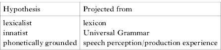
We defer the question of model properties for the moment. As for how something like the SSP comes to be known, we distinguish lexicalist theories – in which the SSP is projected from the lexicon – from universalist theories. The lexicalist hypothesis is consistent with a body of work demonstrating other phonotactic generalisations that are projected from the lexicon (e.g. Frisch & Zawaydeh Reference Frisch and Zawaydeh2001, Hay et al. Reference Hay, Pierrehumbert, Beckman, Local, Ogden and Temple2003). The universalist hypothesis comes in two forms. The most direct form is to posit that the SSP is innate. The innatist approach is common currency in linguistic theory, although for many specific aspects of grammar it is difficult to find a theorist who advocates an innate explanation. The other universal approach that has been proposed is that the SSP is phonetically grounded – learned from experience in producing and comprehending speech, and universal because ‘certain basic conditions governing speech perception and production are necessarily shared by all languages, experienced by all speakers and implicitly known by all’ (Hayes & Steriade Reference Hayes, Steriade and Hayes2004: 1). These possibilities are schematised in Table I.
Explanations for the Sonority Sequencing Principle.

At present, the lexicalist hypothesis is the dominant explanation for phonotactic knowledge: evidence from a variety of methodologies converges on the conclusion that the lexicon is an important seat of phonotactic generalisations. For example, the strength of gradient OCP-Place effects in non-word acceptability judgements is predictable from lexical type statistics (Frisch & Zawaydeh Reference Frisch and Zawaydeh2001; see also Coleman & Pierrehumbert Reference Coleman, Pierrehumbert and Coleman1997). As another example, non-word repetition accuracy is believed to index phonotactic proficiency (Coady & Evans Reference Coady and Evans2008) and is strongly predicted in children by their vocabulary size, consistent with the view that the phonotactic grammar is projected from the lexicon (Edwards et al. Reference Edwards, Beckman and Munson2004; see also Hay et al. Reference Hay, Pierrehumbert, Beckman, Local, Ogden and Temple2003). The question is not whether the lexicon is a source for phonotactic generalisations, but whether it is the sole source.
To show that there is some other source, it would be necessary to find a particular phonotactic generalisation and demonstrate that it cannot be projected from the lexicon. Just such an argument has been made for the SSP, in stronger or weaker forms, by several authors. The argument goes as follows: lexicalist models assign well-formedness on the basis of lexical frequency. Unattested clusters have a frequency of 0. Therefore, lexicalist models should classify all unattested clusters as ungrammatical, and crucially, equally ungrammatical. In other words, they should fail to pick out some (strongly SSP-violating) clusters as more ungrammatical than other (weakly SSP-violating) ones. Sonority projection effects occur, and so lexicalist models are unable to account for them. This argument is made explicitly by Ren et al. (Reference Ren, Gao and Morgan2010: abstract):
The sensitivity to the SSP can hardly be accounted for by lexical statistic factors because Mandarin syllables have no onset clusters and no coda consonants with the exception of [n] and [ŋ], so all the stimuli in our experiments were alien to them. The sensitivity cannot be explained by phonetic confusions either, because similar sensitivity has also been found in reading tasks (Berent Reference Berent2008). The two findings shed light on … basic questions of Generative Grammar by indicating that the SSP, as a Universal Principle, may constitute a part of human linguistic knowledge.
Berent et al. (Reference Berent, Steriade, Lennertz and Vaknin2007) argue similarly. They show that a particular lexical model, the Vitevitch & Luce (Reference Vitevitch and Luce2004) Phonotactic Probability Calculator, has no statistically significant correlation with the results of their sonority projection study. They conclude (2007: 624–625):
Our findings demonstrate that English speakers manifest sonority-related preferences despite the lack of lexical evidence, either direct (i.e., the existence of the relevant onsets in the English lexicon) or indirect (the statistical co-occurrence of segments in English words).
Experimental results along these lines (see also Berent et al. Reference Berent, Lennertz, Jun, Moreno and Smolensky2008, Albright Reference Albright2009) constitute intriguing evidence for the hypothesis that the SSP is not projected from the lexicon. In the theoretical taxonomy of Table I, they may be taken as supporting either the innate or the phonetically grounded hypotheses. However, as Berent et al. (Reference Berent, Steriade, Lennertz and Vaknin2007: 624) point out, the argument relies on the failure of particular statistical models to predict the result, and there is no guarantee that other models will similarly fail. It is this point that we pursue here.
Lexicalist models assign well-formedness on the basis of lexical frequency. The key question, however, is frequency of what? Segments are a natural starting point for phonological analysis, and there is abundant evidence that they represent a psychologically important level of representation. However, segments are not the only representation available for analysis, and from a phonological standpoint, they are not necessarily even the best one. An alternative, noted by Berent et al., is to consider models that employ features, i.e. acoustic and/or articulatory properties that are shared by natural classes of segments.
If a model is limited to counting segments, then it is true that, for example, the onsets [tl] and [lt] are equally unattested. However, from a featural perspective, onset [tl] receives more lexical support than onset [lt]. There are many attested onset clusters that are featurally similar to [tl], e.g. [pl], [kl], [tr], [tw], [sl]. In contrast, there are no attested onset clusters that are equally similar to [lt]. A lexicalist model that generalises across multiple featural levels of abstraction might distinguish degrees of well-formedness between these clusters on this basis, even though the segmental frequency of each cluster is 0. Indeed, at least two lexicalist models have been proposed that generalise on the basis of features: Hayes & Wilson's (Reference Hayes and Wilson2008) Phonotactic Learner and Albright's (Reference Albright2009) featural bigram model. However, there is as yet no published work assessing feature-based computational models for sonority projection (though see Albright, ms).
Thus the goal of this paper is to test a variety of published computational models of phonotactics on this case of sonority projection effects. The value of a direct comparison on the basis of the same stimuli is that we may gain clear insight on what model properties are responsible for success and failure on this particular phonotactic domain, which may inform our understanding as to what collection of properties the next generation of models should have.
In order to assess the predictive utility of a model, it is necessary to have human behavioural data for the model to explain. In this case, the focus is sonority projection effects, and so we begin the paper by collecting non-word acceptability ratings with non-words whose onset clusters vary in the extent of SSP violation. As a matter of general interest, we also included non-words with frequently attested onsets (like [bl]) and marginally attested onsets (like [bw]).
With non-word acceptability data in hand, the paper will proceed to the modelling stage. We implement a number of computational models of phonotactics described in the literature, specifically those in (1).
(1)


The adequacy of the models is assessed by linear regression against the non-word acceptability data.
To anticipate briefly, we find that some published models exhibit considerable success in predicting sonority projection effects. The key findings are discussed in depth later; for now they may be summarised as follows: a lexicalist model can and does predict sonority projection effects if it has (a) the capacity to represent sonority, and (b) a representation of phonological context that is rich enough to represent the expected sonority level. In other words, lexicalist models exhibit sonority projection when they are equipped with the representations and architecture necessary to do so. This work supports a lexicalist account of the SSP.
The paper is structured as follows. In §2, we describe two experiments collecting non-word acceptability judgements from the ‘Mechanical Turk’, an online labour forum. In §3, we give brief descriptions of the computational models tested here, none containing the SSP as a bias. In §4, we describe the results of computational modelling; each model was trained on the same English lexicon and then assessed on its ability to predict human judgements for unattested clusters varying in their degree of SSP violation. In §5, we discuss the empirical findings of this work and their theoretical implications.
2 Sonority projection in acceptability ratings
In this section we describe a non-word acceptability judgement experiment with non-words that were designed to vary in the level of SSP violation. We begin with a summary of sonority scales, followed by a brief description of the Mechanical Turk. The non-words are then described, followed by the acceptability experiment. The experiment had two conditions: in the first condition, participants rated forms on a Likert scale; in the second condition, participants compared two forms and selected the better choice. The section concludes with a theoretical discussion of sonority projection, and a methodological comparison of the sensitivities of Likert rating vs. comparison.
2.1 Sonority scale
To determine whether participants exhibit sonority projection (and whether phonotactic models can explain it), it is necessary to have an independent measure of sonority. A number of sonority scales have been proposed in the literature (e.g. Steriade Reference Steriade1982, Selkirk Reference Selkirk, Aronoff and Oerhle1984, Clements Reference Clements, Dressler, Luschützky, Pfeiffer and Rennison1992, Parker Reference Parker2002), generally having the properties in (2).Footnote 2
(2)
The rise of a sequence XY is defined as sonority(Y)−sonority(X). Then the SSP can be formalised by defining a threshold for acceptable rises, e.g. ‘onsets must have a rise of at least 2’ implies that [bl] is acceptable so long as sonority(l)−sonority(b)≥2. This type of formulation has proven remarkably successful in delimiting onset inventories cross-linguistically (see references above), and is what justifies the assignment of particular integer values to particular segment classes.
Scales proposed in the literature differ chiefly in granularity. Elaborated scales such as Selkirk (Reference Selkirk, Hulst and Smith1982) distinguish obstruent voicing and manner, vowel height and rhoticity. We selected the coarse-grained scale in Clements (1988): obstruents (0)≪nasals (1)≪liquids (2)≪glides (3)≪vowels (4). This scale makes only uncontroversial distinctions representing the consensus of the phonological community.Footnote 3
2.2 The Mechanical Turk
The Mechanical Turk is an online labour forum provided by Amazon.com.Footnote 4 It was used because it offers a quick and easy way to conduct word acceptability and similar studies – the total time to complete data collection was about one hour for each rating method, with a cost of $3 per participant+10% commission for Amazon.com, which compares favourably with 2–3 weeks and $5–$10 per participant for the equivalent laboratory study. Quality is maintained in the Mechanical Turk by the approve/reject option, and the approval threshold. Researchers may reject the work of any individual worker (and refuse to pay); they may also pre-screen by selecting workers whose approval rate is above a threshold; the recommended approval threshold is 95%. As a result, workers and the website are both directly incentivised to ensure an overall high quality of work.
All participants were recruited from the Mechanical Turk using the recommended 95% approval threshold. Participants gave online consent and completed a brief language background survey surveying English proficiency, dialect and other languages spoken. Results were retained from participants reporting ‘high’ English proficiency (Likert rating: n=2; comparison rating: n=12) or ‘native’ proficiency (Likert rating: n=17; comparison rating: n=36). The research team inspected non-native results and found that they exhibited the same qualitative patterns as natives, i.e. attesteds≫marginals≫unattesteds (see the following section for details). Participants reporting ‘intermediate’ proficiency were paid, but their results were discarded and replaced. One (native) participant was excluded from the Likert condition for rating over 80% of the items as ‘1’.
2.3 Stimuli
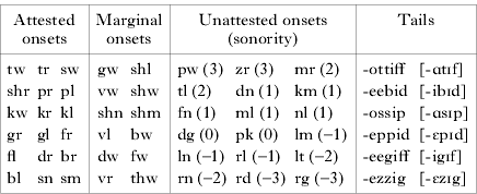
The stimuli consisted of 96 stress-initial CCVCVC non-words, generated by concatenating a CC onset with a VCVC tail (e.g. pr-+-eebid=preebid). There were 48 onsets and six tails. Thus each onset was paired with two tails, and each tail was paired with 16 onsets (48×2=96=16×6). Eighteen clusters that never occur as English onsets (unattesteds) were chosen to vary across the whole range of sonority (e.g. [tl] involves a large sonority rise, whereas [rg] involves a large sonority fall). Also included were 18 clusters that occur frequently as English onsets (attesteds) and 12 clusters that occur only rarely or in loanwords (marginals, e.g. [gw] in Gwendolyn, [ʃl] in schlep). Attested and marginal clusters were included to validate the task (participants should exhibit the preference attesteds≫marginals≫unattesteds) and to increase ecological validity by providing at least some test items that are plausible English words. Six VCVC tails were selected to yield almost no lexical neighbours and to avoid violating any major phonotactic constraints of English.
The list of onsets and tails is shown in Table II, with sonority values in parentheses for the unattesteds.
List of onsets and tails.

The stimuli were counterbalanced in a number of ways. Each tail appeared approximately the same number of times for each sonority range, so that -ottiff, for example, did not appear more often with relatively well-formed unattested onsets. The co-occurrence of tails with onset phonemes was counterbalanced; for example, -ottiff did not appear more often with an onset containing /p/. Repeated segments (e.g. dgeegiff) would be independently dispreferred by the OCP, so these items were avoided as much as possible. Onsets and tails were combined so as to ensure that no non-word had more than one lexical neighbour (neighbour=an existing word obtainable from the non-word by inserting, deleting or substituting one phoneme). To control for embedded words, we avoided non-words whose C1C2VC3 parts formed a real word with attested and marginal onsets; for unattested onsets, non-words whose embedded C2VC3 parts formed a real word were distributed across the sonority range. All of the non-words were presented in English orthography in all capital letters. To ensure that the stimuli were phonologically unambiguous, they were presented to five naive English speakers; all non-words were pronounced as intended, suggesting that the spellings are largely unambiguous.
2.4 Design and procedure
After giving consent and filling out the language background survey, participants completed six practice items, and then performed the main task. All items were presented on a single page, with radio buttons for the answers.
For the Likert rating condition, participants were instructed that they would be rating potential new words of English, that they would see multiple potential words and that they should rate them based on how likely it was that the words could become new words of English in the 21st century. The practice items were stallop, skeppick, thrishal, shmernal, lbobbib and shthokkith, and were intended to expose participants to a wide range of well-formedness. Each item consisted of a single non-word, and the responses were ‘1’ (unlikely) to ‘6’ (likely). Each participant rated all 96 items; four different randomisations were used to control order of presentation effects.
For the comparison rating condition, participants were instructed to choose the non-word that seemed more like a typical English word. The practice items were stallop vs. thmeffle, lbobbib vs. priffin, thrishal vs. ftemmick, skeppick vs. mzibbus, shmernal vs. dwiffert and shthokkith vs. thpellop. Each unique non-word pair was presented to exactly one participant, and each participant was assigned a list of 95 items, so there were 48 participants (96×95/2 pairs=4560 pairs=48 participants×95 pairs/participant). Non-word position (left or right) was counterbalanced, and participant lists were constrained to not contain any non-word more than twice.
2.5 Results
All regressions were done using the lmer() function from the lme4 package (Bates & Maechler Reference Bates and Maechler2009) in R (R Development Core Team 2006). As a check on the task, the entire data set was regressed, using the ordered factor of attestedness (unattested≪marginal≪attested) as the fixed effect. Linear regressions with rating as the dependent variable were used for the Likert condition because the response variable is scalar; onset, tail and participant were included as random effects. Logistic regression was used for the head-to-head condition, with each trial split into two observations corresponding to each of the non-words; the dependent variable indicated whether the non-word was chosen (note that this splitting was necessary because unlike normal logistic regression, the two choices change from trial to trial); onset, tail and participant preference for left/right response were included as random factors.Footnote 5 To determine whether sonority influenced listener judgements, the data sets were restricted to trials containing only unattested clusters. Sonority was used as the fixed effect, but otherwise the regressions were the same as above (linear for Likert, logistic for head-to-head; same random effects).
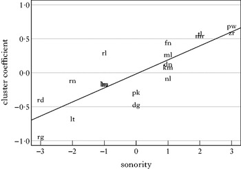
Attestedness was a significant predictor of well-formedness in both conditions. Marginals (non-words containing marginal onsets) were rated significantly higher than unattesteds (Likert: t=−7·4, p<1e−4; head-to-head: z=−6·4, p<1e−9) and attesteds were rated significantly higher than marginals (Likert: t=10·1, p<1e−4; head-to-head: z=6·2, p<1e−9).Footnote 6 In order to show whether there is a sonority effect in the unattested clusters, Fig. 1 plots this regression's unattested cluster random intercepts against sonority. The plot shows that sonority is an excellent predictor of the variance remaining in unattested clusters. The sonority regression confirmed that sonority was a significant predictor of well-formedness for unattested onsets (Likert: t=6·2, p<1e−4; head-to-head: z=7·4, p<1e−12).
Unattested cluster (random) coefficients plotted against sonority.

For modelling purposes, it will prove useful to have a canonical ‘acceptability score’ assigned to each non-word. We define this as the proportion of comparison trials in which a non-word was selected as better than its competitor; this value is used in preference to random intercepts from a regression model, for conceptual transparency and for greater comparability to previous studies (Coleman & Pierrehumbert Reference Coleman, Pierrehumbert and Coleman1997), though the two are highly correlated.
2.6 Discussion
The results of the non-word acceptability experiment demonstrated several important patterns. First, both the Likert rating and comparison conditions exhibited the expected effect of attestedness, with the well-formedness scale attested≫marginal≫unattested; this shows that participants recruited from the Mechanical Turk exhibit the same coarse behaviour as laboratory participants in previous studies. Second, sonority was a significant predictor of acceptability for unattested onsets; this result is consistent with the hypothesis that speakers have internalised knowledge of the SSP, but is hard to otherwise explain. Finally, as discussed below, while both conditions exhibited the same pattern of significant differences, the comparison condition was more sensitive for the unattested items of interest. These points are discussed in turn.
2.6.1 Inclusion of non-native speakers
The results of the present study show that, at a coarse level, participants recruited via the internet exhibit the same behaviour as participants recruited through subject pools or campus flyer. Internet recruitment arguably represents a more ecologically valid sample of English speakers than a study with monolinguals, because a non-trivial percentage of speakers so recruited are early or late bilinguals. This is a potential cause for concern, as even highly proficient late bilinguals may exhibit subtle differences in judgement from native speakers (Coppieters Reference Coppieters1987). Note however that in this experiment the research goal is not to isolate competence of the idealised monolingual English speaker-hearer, but rather to determine whether sonority projection occurs in English non-word acceptability judgements. The other languages our participants reported speaking include Dutch, French, Hindi, Mandarin, Marathi, Punjabi and a few others; these languages are generally as restrictive as or more restrictive than English with respect to onset-sonority profiles. Thus, the sonority-violating clusters in the present study were equally novel to all participants.
2.6.2 Sonority projection
The statistical modelling results showed that sonority is a significant predictor of participants' well-formedness ratings for unattested clusters. The most natural explanation for this finding is that participants have internalised knowledge of the SSP. However it is worth considering the alternative hypothesis that these results reflect some sort of orthotactic knowledge.
The orthotactic account can explain the coarse difference in rating between attested, marginal and unattested onsets, but it fails to explain the effect of interest: sonority projection in unattesteds. The frequency of all unattested onset clusters is (by definition) 0, so they are crucially not differentiated by frequency. Moreover, the visual structure of the English alphabet does not reflect its phonology, e.g. <R> is more visually similar to <P> than to <L>, but more phonologically similar to <L>. The principled relationship between sonority and well-formedness cannot be explained by English orthotactics.
2.6.3 Sensitivity at the bottom of the scale
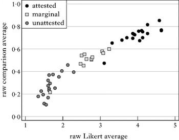
The pattern of significant differences was the same across the Likert rating condition and the head-to-head comparison condition. However, the comparison task was evidently more sensitive for the items of interest, the unattested onsets. One bit of evidence for this claim is that the z statistic for the head-to-head sonority comparison is greater than the t statistic for the Likert comparison, with a corresponding difference in significance (Likert: t=6·2, p<1e−4; head-to-head: z=7·4, p<1e−12). The point can be appreciated more clearly in Fig. 2, which plots raw onset averages from the comparison condition against the Likert condition. (The onset ‘average’ for the comparison condition is defined as the proportion of competitions won by non-words containing the cluster.)
Scatterplot of comparison scores against Likert ratings.

The comparison average differentiates the unattested onset clusters much better than the raw Likert average does. This presumably occurs because the target unattested items are concentrated at the bottom end of the well-formedness spectrum, yielding near-floor ratings for all of them. This fact suggests the following methodological point: in non-word acceptability studies, head-to-head comparison is preferable to Likert rating whenever the stimuli of interest are concentrated at one end of the well-formedness scale, owing to ceiling/floor effects in Likert ratings. Similar conclusions have been reached by Coetzee (Reference Coetzee2008, Reference Coetzee and Parker2009) and by Kager & Pater (ms); and different but related points are addressed in Kawahara (Reference Kawahara2011) ; we mention this methodological point here in the hope of averting unnecessary replication of effort in the future.
3 Computational models of phonotactics
Having established the human behavioural data of interest on sonority projection, we turn now to the question of explaining the judgements that humans make. In this section, we give a brief overview of six computational models that have been proposed to explain non-word well-formedness judgements. The ‘training data’ that will be used here is the lexicon described in §4.1, though in principle these models can train on any lexicon.
3.1 The classical bigram model
Classical bigram models assign probabilities compositionally: the probability of the whole is the product of the probability of the subparts and the way they are combined. In classical bigram models, the subparts are bigrams, and the whole word probability is the product of the transitional probabilities. For example, cat can be expressed as #kæt# (where # is a boundary symbol); its bigrams are #k, kæ, æt and t# (for detailed exposition see Jurafsky & Martin Reference Jurafsky and Martin2009; for a recent linguistic study see Goldsmith & Riggle, to appear). From these, the probability of [kæt] is calculated as in (3).
(3)
The transitional probabilities are estimated from training data using relative frequency; for example p(k→æ) is estimated by dividing the frequency of [kæ] by the frequency of [k]. This model is termed a lexical model, because bigram frequencies are calculated by their type frequency in the training data – in the present study, an English lexicon.
In the natural language processing literature, where bigram and related models are heavily employed, it is considered best practice to smooth the transitional probabilities (Manning & Schütze Reference Manning and Schütze1999, Jurafsky & Martin Reference Jurafsky and Martin2009). Smoothing assigns a modest amount of probability to unseen items, so as to avoid assigning zero probability to items that happen to be absent from the training set.Footnote 7 In our implementation of the classical bigram model, we used Good-Turing smoothing (Gale & Sampson Reference Gale and Sampson1995).
3.2 The syllabic parser
Coleman & Pierrehumbert's (Reference Coleman, Pierrehumbert and Coleman1997) model is similar to a bigram model in that it assigns word probabilities compositionally by multiplying the probabilities of subparts. However, it differs in the subparts: words are parsed not into bigrams but into a phonologically motivated hierarchy consisting of syllables, onsets and rhymes. Separate counts are maintained for stressed vs. unstressed, initial vs. non-initial and final vs. non-final syllables, for a total of eight onset and eight rhyme distributions. Just as in the bigram model, the counts are estimated from the lexicon. Our implementation differs slightly from what is described in the original paper, because our training lexicon includes more than just the binary feet on which the original implementation is based. Therefore, rather than parsing into binary feet, our implementation uses the distribution over all attested stress patterns.
Here is an illustration of how the model computes the probability of the word agenda.
(4)
As with the bigram model, Good-Turing smoothing was used; a separate smooth was done for each onset and rhyme distribution.
3.3 The featural bigram model
Albright's (Reference Albright2009) featural bigram model is broadly similar to the classical bigram model described above. It differs in how the transition probabilities are calculated. Rather than treating each segment as a distinct, unique type, it deploys phonological features, so that each segment may be characterised by any of the natural classes to which it belongs. For example, the segment [b] can be construed as [+labial], [+consonantal], [+labial, +consonantal], [+labial, −nasal] and so on. The likelihood of a bigram is calculated from its ‘best’ natural-class featural description, according to (5).Footnote 8
(5)
The overall rationale of the model is that a word containing populous natural class bigrams are likely to be particularly well-formed, especially when the segments that instantiate the natural class form a large share of that class's population. The rest of the computation works analogously to the classical bigram model.
We ran our own implementation of the model, meant to function identically to Albright's but to facilitate the use of our own feature set and training data.
3.4 The Phonotactic Learner
The Hayes & Wilson (Reference Hayes and Wilson2008) Phonotactic Learner is a constraint-based learning model. Constraints are stated in the phonological vocabulary made standard by Chomsky & Halle (Reference Chomsky and Halle1968) and subsequent work. For example, the constraint *#[+son, −syll][+cons] militates against word-initial [lb] clusters and similar SSP-violating forms. Just as with the featural bigram model, the features allow the Hayes & Wilson model to make generalisations over segments, including generalisations based on sonority.
To assess well-formedness, the Hayes & Wilson model employs the maximum entropy variant (Della Pietra et al. Reference Della Pietra, Pietra and Lafferty1997, Goldwater & Johnson Reference Goldwater, Johnson, Spenador, Eriksson and Dahl2003) of Harmonic Grammar (Legendre et al. Reference Legendre, Miyata and Smolensky1990, Smolensky & Legendre Reference Smolensky and Legendre2006, Pater Reference Pater2009, Potts et al. Reference Potts, Pater, Jesney, Bhatt and Becker2010). Each constraint 픺i has a non-negative weight w i. A word x is evaluated by finding its constraint violation counts 픺i(x), multiplying each violation count by the corresponding weight and taking the sum. The negative of this sum is known as the harmony of x, and the likelihood of x is the exponential of its harmony. To ensure this is a true probability distribution, likelihood is divided by a normalisation constant that guarantees it sums to 1, as in (6).
(6)
The constraints deployed in the grammar are found by a search algorithm that attempts to identify constraints that best explain the training lexicon. The algorithm privileges constraints that are brief (few feature matrices), accurate (low expected/observed violations) and general (covering large numbers of possible forms). The number of constraints that the algorithm includes in a grammar can be set by the user. We caused the model to terminate at 400 constraints, and explored the effect of constraint number by considering subgrammars including only the first 100, 150, 200, 250, 300 and 350 constraints.Footnote 9
3.5 The Phonotactic Probability Calculator
The Vitevitch & Luce (Reference Vitevitch and Luce2004) Phonotactic Probability Calculator is widely used in psycholinguistic research. It resembles several models described already in that it assigns a score to a word by dividing it into parts and combining their probabilities. The model is similar to a bigram model in that it uses bigrams as well their simpler cousin unigrams.
The model employs a positional representation, based on left-to-right serial position of segments. Separate counts are maintained for each position. For example, the probability of [b] as the first segment of a word is based on what fraction of all word-initial segments are [b]; the probability of [b] as the fourth segment of a word is based on what fraction of all fourth-position segments (in words with at least four segments) are [b], and so on. In the bigram version, analogous computations are carried out on bigrams.
The model uses a weighting system evidently intended to provide a compromise between type and token frequency. It weights unigrams and bigrams by the log of their token frequencies, which are rescaled by the total log frequency weight to get unigram and bigram probabilities.
Our implementation reflects the standard practice that has evolved in experimental work making use of this model: a unigram score is calculated as the sum of the unigram probabilities, and a bigram score is calculated analogously.Footnote 10 Note that because the subpart probabilities are not mutually exclusive, summing in this way implies that non-word scores cannot be interpreted as probabilities.
3.6 The Generalised Neighbourhood Model
The Generalised Neighbourhood Model (Bailey & Hahn Reference Bailey and Hahn2001) is an exemplar model in which the well-formedness score of an item is determined directly from the lexicon, by the sum of its similarities to existing words. This is in contrast to the other models discussed above, in which a grammar is first projected from the lexicon, and then well-formedness is evaluated by the grammar.
The similarity of a nonce word ωi to an existing word ωj is calculated from the string-edit distance dij. String-edit distance is calculated from the number of insertions, deletions and substitutions need to change ωi to ωj. As in the original paper, we used an insertion and deletion cost of 0·7, and the proportion of shared natural classes (Frisch et al. Reference Frisch, Pierrehumbert and Broe1997) as the substitution cost. The similarity of ωi to ωj is given by exp(−D⋅dij), where D is a scaling factor. Similarly to Vitevitch & Luce (Reference Vitevitch and Luce2004), log token frequency weighting was included, although this model adopts a more complicated quadratic weighting scheme. The total score for a form is calculated by summing similarities; we differ slightly from Bailey & Hahn (Reference Bailey and Hahn2001) in summing over the entire lexicon, an operation that was not computationally feasible in 2001. The full formula is given in (7).Footnote 11
(7)
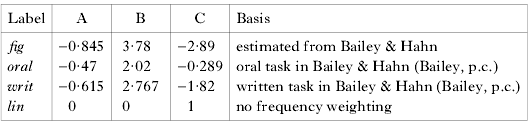
Owing to differences between the training lexicon and test items here and those in Bailey & Hahn Reference Bailey and Hahn2001, we considered several sets of free parameters, as in Table III.
Parameter settings for the Generalised Neighbourhood Model.

3.7 Summary
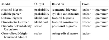
Each of the models discussed in the preceding section is a learning model. It is trained on a lexicon of a language and assigns scalar well-formedness values based on a grammar projected from the lexicon (or based on the lexicon itself). A summary of the models' properties is given Table IV.
Summary of model properties.

For the models whose outputs have a probabilistic interpretation (the first four in Table IV), the outputs were log-transformed. This was partly done for comparison with well-formedness ratings, since Coleman & Pierrehumbert (Reference Coleman, Pierrehumbert and Coleman1997) found that non-word log likelihoods were linearly related to human acceptability judgements; it was also simpler, as the underlying computations are actually performed in the log domain. No such log transform was applied to the scores for Vitevitch & Luce (Reference Vitevitch and Luce2004) and Bailey & Hahn (Reference Bailey and Hahn2001), both for greater comparability to existing studies, and since these values are scalars which do not have a probabilistic interpretation.
4. Modelling non-word acceptability judgements
4.1 Training on an English lexicon
The models described in §3 are lexicalist learning models, meaning that the well-formedness scores they assign are directly or indirectly projected from the lexicon. For a fair comparison, it is necessary to train all models on the same lexicon. This subsection describes the training lexicon.
Our goal was to create a representative dictionary of the words likely to be known to the participants. We used the CMU Pronouncing Dictionary transcriptions,Footnote 12 selecting only those words that have a frequency of at least 1 in the CELEX word-form database (Baayen et al. Reference Baayen, Piepenbrock and Rijn1995). From this set, we removed compounds, residual inflected forms and forms created by highly transparent processes of morphological derivation, yielding a set of 18,612 words in phonemic transcription.
Two versions of the training set were used. In one, syllabification was lexically specified by annotating consonants as belonging to the coda or not.Footnote 13 In the other, coda position was not distinguished in the lexical form. The phonemes of the training set were supplemented by a feature chart.Footnote 14 The feature chart was used by the featural bigram model, the Phonotactic Learner and the Generalised Neighbourhood Model. For these featural models, annotated coda consonants were featurally identical to their onset cousins except they were marked [+rhyme]; for the non-featural models, annotated coda consonants were counted as distinct atomic symbols, i.e. onset [b] was just as distinct from coda [b] as it was from [l].
4.2 Method
Each model was trained on the training lexicon and was then tested on the set of non-words used in Experiments 1 and 2. Training consisted of estimating model parameters as described in §§3.1–3.6. Testing consisted of assigning a well-formedness value to each non-word stimulus.
4.3 Results
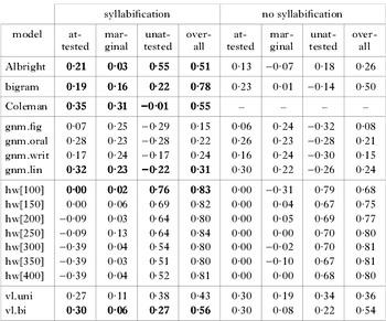
To get a broad overview of model performance, we calculated for each model the correlation of its well-formedness score with the empirically derived well-formedness score from the experimental head-to-head data in §2.5. These correlations are shown in Table V. The focus of this paper is on sonority projection, so what is of most interest is a model's ability to predict variation among the subset of unattested items. However, for completeness and general intellectual interest, we also computed correlations for the attested and marginal subsets, as well as the entire data set. These are reported in Table V.Footnote 15
Correlations of model ratings with Experiment 2 scores. Albright=featural bigram; bigram=classical bigram; Coleman=syllabic parser; gnm.set=Generalised Neighbourhood Model with parameter set; hw[n] = Phonotactic Learner with n constraints; vl.uni/bi=Phonotactic Probability Calculator (unigram and bigram models respectively). ‘Good’ model correlations are given in bold (see text for details).

Models in Table V are arranged in rows, with members of the same ‘family’ adjacent to one another. The columns are divided into two groups, with syllabified training/testing on the left, and unsyllabified input on the right. The columns represent the subset of the data being regressed, and the entries in each cell represent the correlation. For example, the top leftmost numerical cell indicates that the syllabified featural bigram model ratings had a 21% correlation with human judgements on the non-words with attested onsets. These correlations provide a convenient macrolevel summary of the models' predictions.
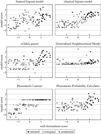
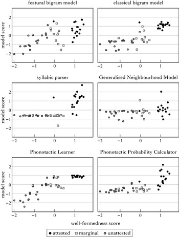
To simplify further analysis, from each family we selected a ‘best’ model, which in our judgement represented the best or near-best performance of that family. For example, hw[100] (syllabified) was selected from the Hayes & Wilson family because it had the (near-)highest attested, unattested and overall correlations. The intention is to focus in on the most informative comparisons – those in which we can be sure relatively poor performance is not simply the result of an unfortunate choice of parameters for a model. Put another way, it is easier to understand six data series than 30, and since many of the data series are parametric variants, it is better to just focus on the six ‘best’ ones. Figure 3 plots model non-word predictions against the comparison judgements from the experiment.
Model non-word predictions vs. human judgements. x-axis: well-formedness score as determined by head-to-head comparison data (z-transformed); y-axis: model score (z-transformed). Each point represents a non-word. Each ‘best’ model is plotted in a different pane.

4.4 Discussion
Several points emerged from the results of the modelling study. The most significant finding for linguistic theory as a whole was that there exist lexical models that explain sonority projection, i.e. predict sonority-related variation in human behaviour for unattested phonological sequences. Among the models tested here, the models which were most effective at modelling sonority projection effects were the Phonotactic Learner (Hayes & Wilson Reference Hayes and Wilson2008) and Albright's (Reference Albright2009) featural bigram model; we will argue that sonority projection owes to a featural representation of sonority and a rich enough representation of context to track the expected sonority profile. Another finding of interest was that no current model excelled across the well-formedness spectrum, i.e. the models that were best on unattested onsets were not best on attested onsets. These points are discussed in detail below.
4.4.1 Sonority projection is possible from the lexicon alone
The most theoretically significant finding of the present study is that sonority projection is achieved by a number of published lexicalist phonotactic models. This finding directly contravenes previous claims in the literature, such as Berent et al.'s (Reference Berent, Steriade, Lennertz and Vaknin2007) conclusion that ‘English speakers manifest sonority-related preferences despite the lack of lexical evidence’. Berent and colleagues have made an important contribution to the field by showing that the SSP is a part of speakers' synchronic knowledge; where we disagree with them is on the claim that there is no lexical evidence for the sonority-based preferences. It is true that, for example, [lb] and [tl] are equally unattested as English onsets, but there are many onset clusters that are featurally similar to [tl], whereas there are none that are so featurally similar to [lb]. As Berent et al. (Reference Berent, Steriade, Lennertz and Vaknin2007: 624) acknowledge, a lexicalist model that is equipped to make generalisations on the basis of features may be able to explain sonority projection; our unique contribution is to show that this is indeed exactly what occurs.
From the belief that there is no lexical support for sonority projection, Berent and colleagues draw the inference that listeners must possess some form of universal knowledge, whether it arises from ‘inherent preferences of the language system’ (2007: 593) or knowledge that is ‘induced from phonetic experience’ (2007: 625). Our results show that the inference of universal, non-lexical phonotactic knowledge does not follow as a logical necessity – although it may still be correct. In short, the ability of a lexical model to explain sonority projection effect bears on foundational issues of our field, because it refutes a powerful argument for the existence of universal phonotactic knowledge.
4.4.2 Model properties needed for sonority projection
Beyond the sheer fact that sonority projection occurs, it is of interest to know why some models exhibit it and others do not. We will argue that what is needed is the ability to capitalise on two representational properties: a sufficiently rich representation of phonological context (e.g. syllabification), and a sufficiently rich representation of sonority itself (e.g. features). The syllabified featural bigram model exhibits sonority projection. However, the unsyllabified featural bigram model does not, so removing syllabification inhibits sonority projection. Similarly, the syllabified classical bigram model does not, so removing featural generalisation also inhibits sonority projection. Thus, sonority projection requires both properties.
4.4.2.1 Phonological context
To express sonority restrictions, a model needs to be able to distinguish contexts that constrain the sonority profile, e.g. it should be rising word-initially. Models trained on syllabified data can do this, since they are told whether a consonant sequence is parsed as an onset, a rhyme or a heterosyllabic cluster. With this information, such models are in a position to inductively track the sonority profiles characteristic of these three contexts, and to characterise well-formedness of these configurations when they are filled by particular segments.
We illustrate using the specific example of the featural bigram model. A cluster like [lt] is perfectly acceptable in English when it is not an onset cluster, e.g. halt, Elton. When syllabification is made available to the model, it should be able to distinguish the unacceptable onset cluster from the acceptable coda and heterosyllabic clusters. Indeed, when it is trained with syllabified data, the Albright model achieves a correlation of r=0·55 with human judgements for unattested onsets. The correlation drops to r=0·18 when the same model is trained on unsyllabified data (we will show later that this level of correlation arises merely from modelling tails). Since the only difference between these two cases is the presence of syllabification, it follows that the contextual information represented by syllabification caused the difference. In other words, syllabification provides a sufficiently rich representation of the context as to allow Albright's model to represent the expected sonority contour.
It is possible for a model to succeed without an explicit representation of syllabification. In particular, with a sufficiently large number of constraints, the Phonotactic Learner achieves roughly equivalent performances on syllabified or unsyllabified data. We believe this is due to the fact that the Phonotactic Learner allows trigram constraints. English trigrams provide a level of phonological context that is more specific than syllabification; for example a trigram model can use structural descriptions of the form [x y C] and [x y #] in place of x coday coda, as was done in Chomsky & Halle (Reference Chomsky and Halle1968). At the same time, scaling up a model to trigrams has its own costs in terms of sparseness of data and computational complexity (Jurafsky & Martin Reference Jurafsky and Martin2009).
In summary, what a model needs is some representation of phonological context that is sufficiently rich as to track the expected sonority contour (see Kager & Pater, ms, for another study concluding that phonotactic models must represent syllabification). Explicit syllabification is an especially simple and effective means of doing this, as evident from the fact that nearly every model does better on nearly every subset of the data when it has access to syllabification.
4.4.2.2 Phonological features
In addition to phonological context, a model needs a system of phonological features. The rationale for this claim is very simple: in order to make generalisations on the basis of sonority, a model must be able to make generalisations, and it must have an explicit representation of segments' sonority. Phonological features perform both of these functions. Features represent inherent generalisations, because the presence or absence of a feature represents an underlying acoustic or articulatory property shared by a natural class of segments. And many of the features commonly used in generative phonology pertain to sonority – for example [+sonorant] segments like [n], [l] and [w] have a relatively open vocal tract providing support for formant resonance, rendering them more sonorous than obstruents like [s], [t] and [tç]. Phonological features are a theoretically convenient way to provide for sonority-based generalisations, because they organise segments into classes on the basis of sonority, and are independently motivated.
The necessity of an explicit representation of sonority can be illustrated by a comparison between the classical bigram and the featural bigram models. These two models differ principally in whether they are designed to generalise on the basis of featural similarity, or to stick narrowly to segmental biphone probabilities. The two models achieve comparable performance on the attested clusters (classical: r=0·19; featural: r=0·21), but differ substantially on unattested clusters (classical: r=0·22; featural: r=0·55). Since the primary difference between these models is whether they make featural generalisations, and the featural bigram model outperforms the classical bigram model on the unattesteds, it is evidently the ability to make feature-based generalisations that causes the difference. In other words, a featural representation of sonority and the capacity to make feature-based generalisations are responsible for sonority projection in Albright's (Reference Albright2009) model.
Extant models that lack a feature system, such as the classical bigram model and the syllable parser, treat segments or other prosodic constituents as atomic units. These models do not ‘know’ that [z] is less sonorous than [l], and so to them there is no or little principled distinction between the onset clusters [zl] and [lz], for example. This seems, almost as a point of logic, fatal to the enterprise of predicting sonority projection to novel clusters. And indeed, all such models achieve at best low correlations with the unattested clusters, which we will argue below arises from modelling the tails. In contrast, the models which employ a feature system – the Phonotactic Learner and the featural bigram model – are exactly the ones with the best success at predicting sonority projection in the behavioural data. Some explicit representation of sonority, such as is generated by a set of phonological features, is a crucial ingredient for making generalisations on the basis of sonority.
4.4.3 Why lexical analogy is insufficient
It is worth asking why the syllabified Generalised Neighbourhood Model (GNM; Bailey & Hahn Reference Bailey and Hahn2001) does not succeed at sonority projection. After all, this model is equipped with a featural representation. As we will show in this subsection, the reason the GNM does not exhibit sonority projection is because even when syllabification is available, the GNM fails to leverage it.
The point can be illustrated most clearly with a slight idealisation. We define GNM′ as identical to the GNM, except that it considers only the closest word in assigning a score. This idealisation is relevant for the non-words in the present study, because the exponent D is quite high, which means that the score is effectively controlled by whatever word(s) have the minimal string-edit distance. Because the non-words in the present study are in sparse lexical neighbourhoods, it is safe to assume that the closest word is unique. Thus for a non-word ν with the existing word ω as a neighbour, the assigned score is GNM′(ν)=exp(−5·5⋅dνω), where dνω is the string-edit distance between ν and ω. Crucially, a non-word's score is determined purely by string-edit distance to its nearest neighbour.
Let us begin with guzu, for which we will suppose guru is the closest neighbour. It is evident that the best string alignment between guzu and guru is the one in which z maps to r and all other segments match. Thus, the string-edit distance between guzu and guru is simply the substitution cost of z→r. For concreteness, let us suppose this is 0·7, which was the insertion/deletion cost in Bailey & Hahn (Reference Bailey and Hahn2001). Then the score assigned to guzu is GNM′(guzu)=exp(−5·5×0·7), because 0·7 is the cost of substituting z→r.
Now let us consider the non-word bzoker, for which we will suppose broker to be the only neighbour. It is evident that the best string alignment between bzoker and broker is the one in which z maps to r and all other segments match. The string-edit distance again consists simply of the substitution cost z→r. Then the score of bzoker is also determined entirely by the cost of substituting z→r. It follows that GNM′ will assign the same score to bzoker as to guzu, namely exp(−5·5×0·7), and moreover it is clear why GNM′ will assign the same score to both non-words – because both differ in exactly the same z→r way from an existing neighbour.
From a phonological perspective, GNM′ assigns the same well-formedness score to guzu as to bzoker; however, guzu is a perfectly legitimate non-word of English, whereas bzoker contains an unattested, sonority-violating onset cluster. The difference in well-formedness is evidently contextual: z is acceptable intervocalically, but not in the onset cluster *bz. Indeed, Albright (Reference Albright2009) notes that the GNM is vulnerable to items like bzeakfast, which overlap strongly with existing words but contain a contextually ungrammatical substitution. We have illustrated here that it is a property of the string-edit metric that the distance between z and r does not depend on context; it treats both z's equally. In other words, context-insensitivity in the underlying string-edit metric implies that the GNM′ is insensitive to phonological context.
For expository purposes, the insensitivity of the GNM to phonological context was demonstrated with an idealised model in which well-formedness is determined by string-edit distance to only the nearest neighbour. However, the idealised model is a good approximation to the true GNM for the non-words in this study, and the insensitivity of the string-edit distance to phonological context holds equally true for the real, non-idealised GNM. Thus, the GNM fails to leverage the phonological contextual information that conditions sonority projection, even when it is provided in the training data.
The reader may wonder why the GNM is actually anti-correlated with human judgements on the unattesteds, rather than simply uncorrelated. The answer lies in what we refer to as delete-initial neighbours. A word y is a delete-initial neighbour to non-word x if y is the closest non-word to x, and the initial segment of y is deleted in the string alignment to x.Footnote 16 For example, the non-word rteppid has tepid as a delete-initial neighbour. In the GNM, the effect of a delete-initial neighbour is to give a boost to a non-word, irrespective of whether its onset is attested or unattested. It is evident from inspection of the GNM pane of Fig. 3 that several non-words with unattested onsets have such delete-initial neighbours. The relevant non-words are rgeebid, rgeppid, lmeebid, rlezzig, dgeppid. These words are concentrated at the bottom end of the well-formedness spectrum, and so the GNM assigns a higher score to a few particular words that are phonologically the least well-formed. This explains why there is actually a negative correlation with well-formedness ratings: our non-word set happened to contain a number of bzeakfast-type items that were concentrated at the bottom of the well-formedness spectrum.
As a side note, the failure of the GNM rules out an important alternative interpretation of the experimental results. Various scholars have raised the issue that non-word acceptability judgements do not reflect pure phonological intuitions, since lexical analogy is known to play a role (Bailey & Hahn Reference Bailey and Hahn2001, Goldrick, Reference Goldrick, Goldsmith, Riggle and Yuin press). We have explained in detail why lexical analogy – at least as it is implemented in the GNM – fails to predict sonority projection, and actually results in anticorrelation with human judgements. This strongly suggests that lexical similarity cannot explain the sonority projection effect we observe for unattested onset acceptability.
4.4.4 The contribution of tails
A reviewer raises the concern that for non-featural models, even small correlations on the unattested items are not predicted under our account (because they do not have featural generalisation). Thus the modest success of the Phonotactic Probability Calculator (r=0·27) and the bigram model (r=0·22) on syllabified training data are of some concern, as are the same models' correlations on unsyllabified training data (r=0·22 and r=0·18 respectively). We will show that these modest correlations arise entirely from modelling the contribution of tails, beginning with Fig. 4.
Model cluster prediction vs. human judgements. Each point represents a cluster. All other graph properties are as in Fig. 3.

Figure 4 isolates the contribution of clusters in the following way. For each model, the contribution of a tail was defined as the average score assigned by the model across all non-words possessing that tail. For each non-word, this contribution was subtracted out from the non-word score. Once the tail contributions were subtracted out, cluster scores were obtained by simple averaging. As with Fig. 3, both x and y coordinates were z-transformed for visual comparison.
It is evident in Fig. 4 that the non-featural bigram models assign essentially flat scores to all the unattested items. The correlation of a constant (model score on unattested onsets) with a variable (human judgements of the same onsets) is zero. Since the models achieve zero correlation on the onsets alone, but a modest positive correlation on the onsets plus the tails, the modest correlations must be caused by modelling the tails' contributions to well-formedness.
Indeed, not only do the non-featural model scores reflect variability from the tails, but they appear to weight the tail contribution too heavily. This conclusion follows from an important difference between human judgements and model scores. Human judgements are dominated by the onset differences. This is evident from the fact that the three attestedness categories are cleanly separated on the x-axis of Figs 3 and 4; it is also evident from Fig. 1, which suggests that onset-sonority profile is the most important predictor of non-word well-formedness. In contrast, the non-featural bigram models sometimes assign higher scores to illegal non-words than to legal ones, as is evident from the fact that the attestedness categories are not cleanly separated on the y-axes of Fig. 3. This fault cannot originate with the onset component of the model scores, since the unattested onset components are essentially flat (as shown in Fig. 4). Therefore the issue must lie with the tails. In other words, a non-word with an illegal onset and a very likely tail (e.g. nlezzig) can be scored better than a non-word with a legal onset and a somewhat likely tail (e.g. sneegiff). For example, the Phonotactic Probability Calculator scores nlezzig as 0·0040 and sneegiff as 0·0028. In non-featural models, the tail component sometimes trumps the onset component, but this does not occurs in our human judgement data.
In summary, the modest positive correlation of the non-featural models on the unattesteds can be attributed to the contribution of the tails, as is evident from factoring out these contributions (in Fig. 4). Moreover, the comparison between Figs 3 and 4 draws out an important weakness of these models – they are too sensitive to the tails: the tail component sometimes trumps the onset component in non-featural model scores, but not in human judgements.
4.4.5 Predicting judgements on attested items
Although the focus of this study is the models' predictions for the unattested items, their predictions for attested onsets are of general theoretical interest as well. As shown in Table IV, the models that achieve the best performance on non-words with attested onsets are the syllabic parser (r=0·35), the GNM (r=0·32) and the Phonotactic Probability Calculator (r=0·30). This finding is of special interest, since these are among the worst models at predicting judgements on the unattested items. In other words, the properties that are necessary for predicting judgements on unattested items are not the same as the properties necessary for predicting judgements on attested items (although there may be some overlap). What, then, is responsible for these relative successes on the attested items?
We believe the property is inherent in the design of these models: conformance to lexical type statistics (e.g. type frequency). This is the essential property that the syllabic parser and Phonotactic Probability Calculator share; and it is directly encoded in the lexical similarity measure of the GNM. For additional theoretical and empirical evidence and argumentation supporting the role of lexical type statistics, see Hay et al. (Reference Hay, Pierrehumbert, Beckman, Local, Ogden and Temple2003) and Edwards et al. (Reference Edwards, Beckman and Munson2004), inter alia.
4.5 Summary
The models that predict sonority projection on the unattested onsets were the syllabified featural bigram model (Albright Reference Albright2009) and the syllabified Phonotactic Learner (Hayes & Wilson Reference Hayes and Wilson2008). We argue that the model properties that underlie this success are (i) a representation of context sufficiently rich as to distinguish expected sonority contour, and (ii) a featural representation enabling sonority-based generalisations. Models that lack either of these properties – or the ability to exploit them in the proper way – will fail at sonority projection. For example, the GNM fails because the string-edit metric is not sensitive to phonological context. The modest positive correlations in Table V of some models not possessing both properties can be attributed to modelling variation in the tails; comparison between Figs 3 and 4 shows that these models overweight the contribution of tails relative to human judgements. Finally, the models which do best at predicting judgements on unattested onsets are among the worst at predicting judgements on attested onsets; apparently what is needed for attested items is conformance to lexical type statistics or lexical analogy.
5. Pushing the lexicalist account to its limits
It has been argued that sonority projection effects in Korean (Berent et al. Reference Berent, Lennertz, Jun, Moreno and Smolensky2008) and Mandarin (Ren et al. Reference Ren, Gao and Morgan2010) provide evidence against the lexicalist account. The argument runs as follows. (i) Korean and Mandarin lack onset clusters. (ii) Lexicalist accounts predict that a language must have consonant clusters in order to induce the SSP. Therefore the lexicalist account predicts no sonority projection effects in these languages. (iii) Sonority projection effects are evident in Korean (Berent et al. Reference Berent, Lennertz, Jun, Moreno and Smolensky2008) and Mandarin (Ren et al. Reference Ren, Gao and Morgan2010). (iv) So the lexicalist account makes an incorrect prediction. We do not dispute the existence of sonority projection effects in Mandarin and Korean, or that conclusion (iv) follows if (i)–(iii) are true. However, we will show here that (i) is questionable and (ii) is false. Both languages could be analysed as having surface obstruent–glide clusters, so it is not clear these languages are the proper test case. However, even if they are, modelling results show that sonority projection can be explained even from exposure to a CV language.
We will begin with the phonological analysis of Korean and Mandarin. We take it as uncontroversial that Korean and Mandarin allow syllables whose onset and nucleus jointly contain three segments, such as the family names Choi (Korean) and Huang (Mandarin). These items are traditionally analysed (e.g. Hockett Reference Hockett1947: 223) as containing diphthongs in which the second segment is affiliated to the nucleus: [tɕuæ], [huaŋ]; under this analysis, it is true that both languages lack onset clusters. However, there are good reasons to analyse these items as having complex, obstruent–glide onsets: [tɕwæ], [hwaŋ] (Korean: Lee Reference Lee and Kim-Renaud1994; Mandarin: Duanmu Reference Duanmu2000: 86). For example, Korean generally allows labial and coronal approximants in the onset position, but specifically disallows them before the structurally ambiguous segment in question (*[juæ], *[wiæ]); this absence has every appearance of a sonority effect, and could be taken as evidence for the complex onset analysis if the SSP is construed as regulating the onset profile specifically. Since it is a priori reasonable for learners to entertain the hypothesis that such sequences are surface clusters, and some aspects of the data arguably favour this hypothesis, the claim that Korean and Mandarin lack complex onsets is not really clear-cut.
Even if sonority projection were demonstrated in a strict CV language, Hayes (in press) shows this does not demonstrate the need for universal (non-lexical) phonotactic knowledge. This point was demonstrated using simulations with the Phonotactic Learner on artificial languages called Ba and Bwa. Ba consisted of every possible CV syllable; Bwa included all CV syllables as well as all possible syllables with a stop–glide onset (hence the name Bwa). The segmental inventory, arranged by sonority class, was [p t k b d g] (stop)≪1 [f v s z] (fricative)≪2 [m n] (nasal)≪3 [r l] (liquid)≪4 [w j] (glide)≪5 [a] (vowel). The integers here are for expository convenience and represent the divisions between classes on the sonority scale, as follows: [−son α] represents all segments below breakpoint α, e.g. [−son 2] represents the stops and fricatives. The Learner was endowed with two families of ‘sonority-regulating’ constraints, i.e. those in which some minimal difference between the initial and the final consonant of the cluster is enforced.
(8)
Crucially, the constraints included both SSP-enforcing constraints and their exact opposites. For example, *[+son 4][−son 1] bans glide–stop clusters like rd; *[−son 1][+son 4] bans stop–glide clusters like dr. Sonority projection was identified as the presence of a gradient of well-formedness across C1C2 clusters, in which well-formedness increased with the sonority of C2, and decreased with the sonority of C1. Hayes (Reference Hayesin press) finds sonority projection in Bwa, indicating that the presence of just obstruent–glide clusters is enough to trigger sonority projection. Crucially, Hayes also found sonority projection in Ba, indicating that sonority projection from the lexicon may occur even without clusters in the input. This arose because featural generalisation of the sharp sonority rise from C to V results in a sonority-dependent gradient of well-formedness for C to C.
In summary, the claim that Korean and Mandarin lack complex onsets is problematic. Even if this analysis is accepted as the one that learners definitely make, the existence of sonority projection in these languages does not clearly refute the adequacy of a lexicalist model. Hayes (Reference Hayesin press) demonstrates that the Phonotactic Learner exhibits sonority projection on CV languages when it is equipped with constraints that include both the SSP and its exact opposite. The existence of sonority projection in these languages therefore does not demonstrate the need for, or existence of, universal (non-lexical) phonotactic knowledge.
6. Discussion and conclusions
We conclude the paper with a summary of the major findings and brief discussion. In summary, we have shown that:
(i) Sonority projection is evident in non-word acceptability studies. Head-to-head comparison is appropriate because the target stimuli are concentrated at the bottom end of the well-formedness scale.
(ii) To explain sonority projection, any phonotactic model must be equipped with a featural representation of sonority and a representation of phonological context such as syllabification.
(iii) When so equipped, lexicalist models with the capacity for context-sensitive featural generalisation can and do explain sonority projection. English well-formedness judgements on SSP-violating clusters were well modelled by the Phonotactic Learner (Hayes & Wilson Reference Hayes and Wilson2008) and Albright's (Reference Albright2009) featural bigram model.
(iv) The existence of sonority projection effects in Mandarin and Korean (Berent et al. Reference Berent, Lennertz, Jun, Moreno and Smolensky2008, Ren et al. Reference Ren, Gao and Morgan2010) does not falsify the lexicalist account, as sonority projection can be explained by a lexicalist model exposed only to CV syllables.
The latter two points refute arguments against the lexicalist account that have been interpreted as powerful support for universal (non-lexical) knowledge of the SSP. Thus the results in this paper bear on foundational issues of our field. In the remaining sections, we enlarge on some of these points.
6.1 Sonority and context are needed for sonority projection
We have argued that a representation of sonority and context are needed for a lexicalist model to exhibit sonority projection. However, there is nothing in the theoretical arguments we made that is specific to lexicalist models. Rather, this point should obtain for all phonotactic models that predict sonority projection. To exhibit gradient sensitivity to degree of sonority violation, a model must have a gradient representation of sonority, such as a standard featural scale. And since the sonority profile intrinsically depends on at least two segments and their relation to the nearest sonority peaks, a model must represent this context in order to predict the expected sonority contour. These points do not depend on where knowledge of the SSP comes from (lexicon, phonetic experience, innate, etc.); rather they refer to properties of the representation that a model must have to adequately explain human performance.
6.2 Lexical models that generalise succeed with sonority and context
In the preceding section we summarised arguments to the effect that any phonotactic model must have a gradient representation of sonority and an adequate representation of phonological context in order to explain sonority projection effects. The most significant empirical contribution of this paper is to show that when a model has these properties, and the capacity to make generalisations on the basis of them, it may succeed at sonority projection. Our results refute the view that lexicalist models are unable to explain sonority projection and humans must therefore possess some universal knowledge of the SSP. For example, the model that Berent et al. (Reference Berent, Steriade, Lennertz and Vaknin2007) used was the Phonotactic Probability Calculator (Vitevitch & Luce Reference Vitevitch and Luce2004). We have shown here that the problem was not that its predictions were derived from lexical frequencies, but rather that it lacked the capacity for generalisation based on sonority, because its computations were based on atomic representations of segments that excluded sonority.
In the present paper, we have shown that models that possess both a featural representation of sonority and the capacity for feature-based generalisation do in fact predict sonority projection. The relevance of these properties was empirically demonstrated by ‘minimal model pairs’. Albright's (Reference Albright2009) featural bigram model with syllabified input succeeded at sonority projection (= adequately modelled sonority-based variation in human judgements on non-words with unattested onset clusters). In contrast, the featural bigram model without syllabification lacked an adequate representation of context, and it failed. The classical bigram lacked a featural representation of sonority from which to generalise, and it failed. Since these models are otherwise identical in their essentials to the featural bigram model with syllabification, it must have been syllabification and featural generalisation specifically that caused success in the one case, and their absence that caused failure in the other cases.
In summary, we have offered both theoretical and empirical arguments for our core position: when a lexicalist model is equipped with the necessary properties of a featural representation of sonority and an adequate representation of context, it not only can but does explain sonority projection.
6.3 Synchrony, diachrony and the SSP
We began this paper by posing the questions of what properties any phonotactic model must have, and where knowledge of the Sonority Sequencing Principle comes from. In the present paper, we have argued that synchronic knowledge of the SSP may derive from the lexicon; moreover we have shown that the English lexicon provides a great deal of support for the SSP. However, there is a significant challenge remaining under the hypothesis that the SSP does in fact derive from the lexicon: why is the SSP an apparent typological universal?
Under both the innatist and phonetically grounded accounts, the universality of the SSP is transparently accounted for. Under the innatist account, universality is accounted for by the assumption that the SSP is part of our common human endowment of UG. Under the phonetic grounding account, sonority projection derives from the speaker-hearer's implicit knowledge of articulatory and perceptual relations, e.g. the onset rt is dispreferred both because of the articulatory difficulty of initiating, pausing and then re-initiating voicing, and because the perceptual cues to the presence of a word-initial r are obfuscated by the following obstruent (for a summary of perceptual cueing see Wright Reference Wright and Hayes2004). This knowledge is universal because we all share the same articulatory and perceptual mechanism. In either case, it is clear why the SSP is universal.
In contrast, the lexicalist hypothesis is that the SSP emerges from the lexicon. Thus, the SSP should only be universal if there is some process that universally causes lexicons to prefer words that are in conformance with the SSP. The lexicalist account does not in itself explain why lexicons are cross-linguistically structured so as to support the SSP, as the null hypothesis is that lexicons are subject to arbitrary variation (for discussion see Prince & Smolensky Reference Prince and Smolensky1993 and Joseph Reference Joseph1995), including conformance to the SSP. Since they are not, the lexicalist hypothesis must be supplemented with some diachronic hypothesis that explains why SSP-conforming words come to predominate in the lexicons of the world's languages.
The obvious candidate is Evolutionary Phonology (Blevins Reference Blevins2004). Evolutionary Phonology proposes that sound patterns are ‘phonologised’ when a gradient phonetic phenomenon is analysed as an automatic, categorical process. A crucial aspect of Evolutionary Phonology is that it posits that phonology is not ‘teleological’, i.e. phonetically unnatural patterns (such as the English k~s alternation embodied in electric~electricity; Pierrehumbert Reference Pierrehumbert, Goldstein, Whalen and Best2006) can be phonologised just as easily as phonetically natural ones like nasal place assimilation (for additional examples see Baroni Reference Baroni2001, Koo & Cole Reference Koo, Cole and Botinis2006 and Kawahara Reference Kawahara2008). Under this account, the reason that phonetically natural patterns are more likely to be phonologised is because they occur more frequently. Thus Evolutionary Phonology differs crucially from the phonetic grounding account in locating some language universals in the conditions governing speech production and perception in the world, rather than the grammar in the minds of speaker-hearers.
A detailed proposal of how Evolutionary Phonology could account for the predominance of SSP-conforming words in a lexicon is beyond the scope of the present paper. However, the general idea seems clear. Suppose that a lexicon begins with a number of SSP-violating words, as well as a number of SSP-conformers. As documented by Blevins (Reference Blevins2004) and others, the phonetic factors governing speech perception and speech production might cause misperception and misproduction more frequently in the SSP-violators. For example, sonority-violating clusters might be more likely to be both produced and perceived with an epenthetic vowel even though the offending clusters are legal in the language (Berent et al. Reference Berent, Steriade, Lennertz and Vaknin2007). Such words might gradually acquire an underlying vowel that repairs the difficult cluster. Thus the lexical support for these clusters is gradually eroded, with the end result that they become unattested.
This sketch is different from the phonetically grounded account, but not incompatible with it. Under the phonetically grounded or innatist accounts, knowledge of perceptual and articulatory difficulty is encoded in the grammar, i.e. ill-formedness is mentally represented. Under the Evolutionary Phonology-style account, evolutionary selection favours SSP-conforming words even if ill-formedness is not mentally represented. This is necessary to avoid circularity – we could hardly claim that the lexicalist account avoided the need to posit universal phonotactic knowledge if it appealed to an evolutionary account that assumed universal phonotactic knowledge. Thus it is necessary that the Evolutionary Phonology account could explain the lexical universality of the SSP even without universal (non-lexical) knowledge, i.e. that SSP-conformers are evolutionarily selected for even without an intrinsic grammatical preference. However, the fact that the Evolutionary Phonology account can explain the lexical universality of the SSP without grammatical universals does not thereby imply that we believe universal accounts are incorrect. Indeed, we suspect that ultimately the SSP will prove to derive from a combination of lexical and universal (non-lexical) knowledge.
6.4 The next generation
Beyond the theoretical contribution to our understanding of the SSP, the results of the simulations here suggest a promising outlook for the next generation of phonotactic models. Recall the finding that the models that did best on the unattested onsets were not those that did best on attested onsets. Moreover, we offered informed opinions as to which properties were responsible for success on each domain. The models with featural generalisation did best on unseen, ungrammatical items, while the remaining models whose computations were based on lexical type statistics did best on non-words whose parts were all attested. These properties are not inherently mutually exclusive.
Therefore, it is tempting to believe that a better model could be built by incorporating the best properties for both domains. For example, the Phonotactic Learner currently assigns essentially flat scores to all non-words that are relatively well-formed. It is quite likely that this outcome derives from search biases built into the model that were explicitly intended to help it find exceptionless constraints (Hayes & Wilson Reference Hayes and Wilson2008), and that the model would also distinguish gradient well-formedness predictions on attested items if these biases were relaxed. Similarly, the featural bigram learner here does less well than the classical bigram on non-words whose subparts are all attested. Presumably this occurs because the model allocates too much probability mass to featural generalisation, when on attested items it would do better to simply abide by the existing lexical statistics. Analogously, the GNM could be improved by using a similarity metric that is sensitive to phonological context. In short, the model properties needed for unattested items are not mutually exclusive with the properties needed for attested items; there is nothing principled standing in the way of the next generation of models incorporating both types of properties.