I. INTRODUCTION
The crystal–melt interface is of great importance in the study of crystal nucleation and growth.Reference Turnbull1–Reference Dullens, Aarts and Kegel12 Despite the fundamental value and the practical application in determining material properties, acquiring interfacial free energy accurately remains a challenge. TurnbullReference Turnbull1 proposed an empirical relation between the latent heat of fusion and the interfacial free energy from which the crystal–melt interfacial free energies from experiment for various materials from homogenous nucleation rates at their maximum undercooling temperatures were extracted. However, this approach cannot be used to determine the anisotropy of the interfacial free energy well due to the approximations inherited from the classical nucleation theory. Another approach, grain-boundary groove experiments,Reference Gündüz and Hunt13–Reference Keşlıoğlu, Gündüz, Kaya and Çadırlı15 examines the shape of the interface where it intersects with a grain boundary, from which more accurate interfacial free energy can be directly extracted. Unfortunately, such experiment requires transparency of the samples. As a result, so far only a few materials have been studied using this approach.
Compared with experiment, computer simulation has become the method of choice in determining interfacial free energy and its anisotropy from atomic scales. A popular approach, the capillary fluctuation method (CFM) has been used and applied to a number of model systems.Reference Hoyt, Asta and Karma16–Reference Potter and Hoyt35 Interfacial free energy and its anisotropy are calculated by examining the capillary fluctuation of the magnitude in a profile of an interface. This technique usually has two steps: first, creating a crystal–melt interface and second, accurately extracting interface profiles. In some simulations,Reference Morris and Song21,Reference Mu, Houk and Song23,Reference Feng and Laird27 crystal and melt slabs were prepared separately, and joined together afterward to form a crystal–melt interface. However, in this case, the atoms at or near the interfaces may be too close to each other and introduce strong repulsive forces, which may lead to nonuniform stress on interfaces. Morris et al.Reference Morris, Wang, Ho and Chan36 have discussed some of the issues associated with the method, including the drift of the solid–liquid interfaces. Naturally, unstable crystal–melt interfaces can lead to inaccurate melting temperature and, therefore, affect the result of interfacial free energy calculation. In this study, we used a different approach in creating crystal–melt interfaces by introducing an extra Lennard-Jones (LJ) potential that alter the force field of crystalline atoms, albeit only transient, and obtained stable interface profiles. With the methods mentioned above, we managed to get reliable melting temperature and interfacial free energy for different crystal–melt interfaces. The study is organized as follows. In Sec. II, we briefly outline the capillary fluctuation approach and the models used in our simulations. In Sec. III, results are presented with discussions. Conclusions are shown in Sec. IV based upon our results.
II. THEORY AND APPROACH
A. Theoretical background
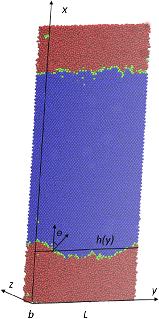
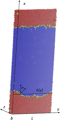
As illustrated in Fig. 1, a quasi-three-dimensional system, with the length of the interfaces L much larger than the thickness b, is made of three parts: crystal (blue), melt (red), and interface (green). The interfacial orientations can be denoted with respect to the crystallographic reference frame of the crystal as (ijk)[lmn], where (i, j, k) is the vector normal to the interface (x axis) and [l, m, n] is the vector tangent to the interface along the short direction (z axis). The interface profile (average over the thickness along the z axis) is given by a function x = h(y) for each of the two crystal–melt interfaces.
A snapshot of the system with two (100) interfaces. Blue atoms have a larger value of order parameter, whereas red atoms have smaller values. The green atoms are defined as interface atoms with order parameter between blue and red atoms. The coordinate axes are shown here with respect to the crystallographic orientations. In the [001] direction (normal to the figure or the z axis), the periodic repeat distance is significantly shorter than in the other two directions. θ is the angle between the interface normal and the x-axis.

Thus, we can cast the interface into a two-dimensional function x = h(y) effectively. The variation of the interface height, or fluctuation represented by h(y), is related to the stiffness of the interface, or rigidity. For a macroscopically rough interface, the size of the capillary fluctuation modes is related to the interfacial stiffness γ̃ by the equipartition theoremReference Karma37:
 $$\tilde \gamma \left( k \right) = {{{k_{\rm{B}}}T} \over {bL\left\langle {{{\left| {A\left( k \right)} \right|}^2}} \right\rangle {k^2}}}\quad ,$$
at a given temperature, where the wave number k takes values k = 2πK/L, with K = 1, …, N. The k-th Fourier mode of capillary fluctuation, A(k), is defined as follows:
 $$A\left( k \right) = {1 \over L}\int\limits_0^L {h\left( y \right)\exp \left( {iky} \right){\rm{d}}y} \quad ,$$
and the interfacial stiffness is given in terms of the interfacial free energy by the formula
 $$\tilde \gamma \left( \theta \right) = \gamma \left( \theta \right) + {{{{\rm{d}}^2}\gamma } \mathord{\left/ {\vphantom {{{{\rm{d}}^2}\gamma } {{\rm{d}}{\theta ^2}}}} \right. \kern-\nulldelimiterspace} {{\rm{d}}{\theta ^2}}}\quad ,$$
where θ is the angle between the instantaneous local normal of the interface and the average orientation of the reference flat interface (see Fig. 1). Based on the cubic harmonic expression from Fechner and Vosko,Reference Fehlner and Vosko38 the interfacial free energy and its anisotropy is determined by
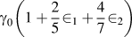
 $$\gamma \left( \bi{n} \right) = {\gamma _0}\left[ {1 + { \in _1}\left( {\mathop\sum\limits_i {n_i^4 - {3 \over 5}} } \right) + { \in _2}\left( {3\mathop\sum\limits_i {n_i^4 + n_1^2n_2^2n_3^2 - {{17} \over 7}} } \right)} \right]\quad ,$$
where {n 1, n 2, n 3} are the Cartesian components of the unit vector n normal to the interfacial plane; γ0 is the orientationally averaged interfacial free energy; and ϵ1, ϵ2 are the expression coefficients. A similar expression for the stiffness can be derived using Eq. (3). By simulating a number of interfaces with different crystal orientations and measuring the average magnitude of the fluctuation modes, the interfacial stiffness γ̃ could be determined from Eq. (1), then one can compute γ0, ϵ1 and ϵ2 and interfacial energy by using Eqs. (3) and (4).
As seen above, the CFM naturally fit for finding the anisotropy, although the interfacial stiffness is highly sensitive to the small anisotropy in γ. For completeness, we provide expressions for γ and γ̃ for the orientations studied in this work in Table I.
Simulated system sizes and expressions of interfacial free energy and stiffness for different interface orientations.

B. Creation of stable crystal–melt interface and its melting point
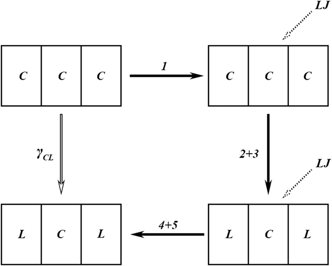
In this work, we use aluminum as a test example. The potential Al1, a kind of embedded atom method (EAM) interatomic potential used in our simulations from Mendelev et al.,Reference Mendelev, Kramer, Becker and Asta39 is considered. A number of melt properties were included in the fitting of the potential, which is more suitable for the problems addressed here. As mentioned above, one of the big challenges in using CFM is to obtain a stable solid–liquid interface. Therefore, the fluctuation detected is ensured that comes from the true interface height variation rather than metastable or unstable change of the interface. Previous work used the methods to create interface by directly bringing a liquid and solid in contact.Reference Morris and Song21,Reference Mu, Houk and Song23,Reference Feng and Laird27 In doing so, it is not guaranteed that the interface contact is optimized, i.e., no atom overlapping caused repulsion and no other big perturbation caused metastability. To resolve this problem, we introduced an extra, variable LJ potential for creating crystal–melt interfaces. A similar version of this method was used in creating stable crystal–liquid interface in an early study.Reference Bai and Li40 The procedure is illustrated in Fig. 2. Here “C” denotes the crystal and “L” denotes the melt. A typical simulation contained 38,400–64,000 atoms. MD runs were carried out in the NPT ensemble, where N is the number of particles, P is the pressure which is set to zero, and T is the temperature. The time step is set as 1fs.
Schematic representation of the five step CFM process used to obtain the crystal (C)–melt (L) interfacial free energy.

Initially, the atoms were arranged in fcc lattices in step 1. The system was divided into three parts and a LJ potential with specific well depth, 0.04 eV in our work, was added to the middle part of the crystal, in addition to the EAM potential for Al. At the interface region, another LJ potential was added to atoms with the well depth of 0.02 eV. Afterward all the atoms were relaxed for 100 ps at 930 K. In step 2, the whole system was heated up to 1150 K in 300 ps. As the temperature was higher than the melting temperature, atoms in the left and right parts became melt. In the middle part, however, atoms still remain in the crystalline state because of the presence of the extra LJ potentials. In step 3, after a short time period of 20 ps of equilibrium and relaxation, the system was cooled down to a temperature close to 930 K in 200 ps (step 3). In the final step, the LJ potentials were removed gradually in 500 ps and we are left with a sample with two co-existing crystal and liquid phases and two crystal–liquid interfaces at two sides of the crystal in the middle. This method ensures that we have stable interfaces; otherwise, the heating and cooling makes it very difficult, especially when interfaces with slightly different interface energies.
Subsequently, we monitored the movement of the crystal–melt interface at different temperatures. If the interface moved toward the melt side, which is the sign of crystallization of the melt, we then slightly increased the temperature, or vice versa. After a series of trial and error, the interface became stationary, which gives also the melting point associated with the interface. Subsequently, snapshots of the interface profiles were collected every 1 ps for a total of 2000 configurations for calculation of the interface free energy using CFM.
C. Extraction of interface
After stable crystal–melt interfaces are obtained, one needs to extract the interface profile h(y). If the values of the function h(y) were measured at a discrete set of points y n = nΔ, where n = 1, …, N, and Δ = L/N is the width of bins, y n. Then Eq. (2) becomes
 $$A\left( k \right) = {1 \over N}\mathop\sum\limits_{i = 1}^N {h\left( {{y_n}} \right)\exp \left( {ik{y_n}} \right)} \quad .$$
To determine the interface profile h(y n), we introduced an order parameter ψi for each atom, proposed by Morris.Reference Morris20 Firstly, the local order parameter for each atom was calculated via
 $${\psi _i} = {\left| {{1 \over {{N_{\rm{q}}}}}{1 \over Z}\mathop\sum\limits_r {\mathop\sum\limits_q {\exp \left( {iq \cdot {r_{ij}}} \right)} } } \right|^2}\quad ,$$
where N q is the number of reciprocal vectors of perfect fcc lattice. In our simulations, four reciprocal vectors along (111) direction were selected. Z = 12, denotes the nearest neighbors of each atom i, and r ij = r j − r i is the distance between two atom at rj and ri. The order parameter is 1 for the perfect crystal and 0 for melt. To reduce the effects of molecular vibrations due to thermal fluctuations and to improve the discrimination between the crystal and melt phases, an average order parameter for each atom is used as follows,
 $$\bar \psi = {1 \over {Z + 1}}\left( {{\psi _i} + \mathop\sum\limits_j {{\psi _j}} } \right)\quad ,$$
where j runs over all nearest neighbors (Z). According to the values of their order parameters, atoms are classified into three categories: the atoms whose order parameters fall into [ψmin, ψmax] were identified as interfacial atoms, the atoms with order parameter larger than ψmax and less than ψmin were denoted as crystal atoms and melt atoms, respectively. ψmin and ψmax are the lower and upper bound values of the order parameter that will be specified later.
Therefore, h(y n) in Eq. (5) could be calculated as the average position of “interfacial atoms” marked by proper order parameters. Even though Eq. (1) implies that γ̃(k) should be independent of k, there are still deviations for both small and large k. This is because the relaxation time increases with the mode length,Reference Morris20 and can be very large compared to the simulation time for small k (large wave length), thus leading to under-sampling and larger uncertainty in the obtained results. The relationship between the stiffness and the average size of the fluctuations shown in Eq. (1) also no longer works when the wave length becomes comparable to the crystal lattice spacing, due to the failure of the assumption of the continuous interface profile. Based on these considerations, we therefore expected to see a k-independent behavior of γ̃(k) only in a limited range k in the range [k min, k max]. Then the interfacial stiff γ̃ can be obtained as the value γ̃(k) averaged over k in this range.
III. RESULTS
The equilibrium temperatures of coexisting crystal–melt phases are given in Table II. It is found that the average melting temperature is 934.79 K, which agrees well with the experimental value 933 K.Reference Smithels41 As known, the melting temperature depends on the orientation of interface. For example, the interface with orientation (100)[001] corresponds to a lowest temperature 929.22 K whereas (110) $\left[ {1\bar 10} \right]$ to 940.10 K, the highest temperature detected so far. The anisotropy of the melting temperature is related to the atomic packing of an interface; more dense, the higher the melting point.
Melting temperature and calculated interfacial free energy, interfacial stiffness for interfaces with different orientations (the values in brackets indicate the 95% confidence intervals, detailed analysis is shown in appendix).

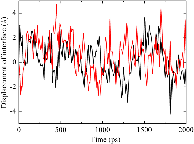
The mean interface position of the orientation (100)[001] in simulation is shown in Fig. 3. The interface was chosen by averaging the positions of the interfacial atoms whose order parameters fall in the range of 0.20–0.40. Figure 3 shows that the movement of the interface is stationary with fluctuations to the left and right. The fluctuation is random throughout the simulation with the displacement no more than 4 Å, as also reported by Hoyt et al.Reference Hoyt, Trautt and Upmanyu42
The interface position is plotted as a function of the simulation time. The black line represents the interface position at the left of the crystal phase whereas the red line represents the one at right. Within 2000 ps, the maximum displacement of interface is no more than 4 Å, comparable to the lattice parameter.

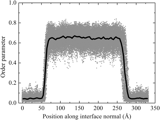
Figure 4 shows the order parameter  $\bar \psi$ for each atom along the x-direction in a system with coexisting crystal and melt phases. The variation of the order parameter can be seen as a function of distance across the interfaces. As seen in the figure, the melt region has the order parameter of $\bar \psi$ < 0.2, whereas the crystal region with $\bar \psi$ > 0.4 and the average value < $\bar \psi$ > ≈ 0.65.
The order parameter versus position for each atom in an instantaneous configuration of two (100) interfaces, as a function of atomic position measured along the interface normal. The center region, where the order parameter is larger, is crystal, whereas the regions where parameter is small correspond to the liquid region.

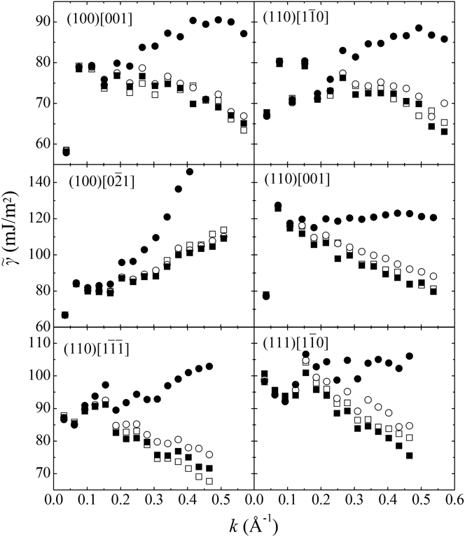
To obtain the interface stiffness, locating the interface profile is particularly crucial. However, in simulation, the interface profile is strongly dependent on the values of ψmin, ψmax chosen. It is a challenge to obtain a reliable and true interface profile. To this end, we investigated the dependence of the interfacial stiffness based on the choice of the threshold ψmin, ψmax, which is shown in Fig. 5. For the interface with orientation (100) $\left[ {0\bar 21} \right]$, if the gap between ψmin, ψmax is selected too larger (0.20–0.40), the interfacial stiffness would increase quickly as we increase the value of k, while narrower gaps (0.2–0.3, 0.25–0.35, 0,30–0.40) correspond to stable stiffness. However, for other orientations, the interfacial stiffness decreases with k in narrow gaps, and becomes stable at 0.2–0.4. Because interfacial stiffness γ̃(k) should be independent of k from Eq. (1), the favorable threshold should lead to stable value of γ̃ for different k. Therefore, we selected the threshold 0.25–0.35 for the orientation (100)
 $\left[ {0\bar 21} \right]$, and 0.20–0.40 for other orientations.
The stiffness of the fluctuation modes evaluated using different order parameters. Open squares (□) represent parameter between 0.2 and 0.3, whereas open circles (○) represent parameter between 0.25 and 0.35. Solid squares (■) and solid circles (●) correspond to parameter 0.30–0.40 and 0.20–0.40, respectively. The results are averaged over 2000 samples of the interfacial profiles and over the two interfaces in each system, the bin width Δ was selected as 2 Å.

The stiffness values obtained are presented in Table II, with error indicating 95% confidence intervals. The detailed error analysis will be given in the appendix. The interface with the orientation (110)[001] provides the largest stiffness value of 119.99 mJ/m2, about 40 mJ/m2 larger than the (110) $\left[ {1\bar 10} \right]$ interface. Although the stiffness values of the (100)[001] and (100)
 $\left[ {0\bar 21} \right]$ interfaces have the same expression (Table I), we see a difference of about 8 mJ/m2 between the two orientations. To obtain these results, as discussed earlier, we restrict the averaging to within the interval 0.1 < k < 0.5, because otherwise the calculated stiffness varies with k values. We also investigate the dependence of the stiffness on the bin width Δ. It is found that the wider Δ is, the higher the values of computed stiffness γ̃(k) for large k, which agrees with the work of Davidchack et al.Reference Davidchack, Morris and Laird24 Therefore, we selected Δ of 2 Å as presented in Fig. 5.
Fehlner and Vosko parameter are calculated by applying linear regression using stiffness values from the six orientations, which are γ0 = 98.35 mJ/m2, ϵ1 = 3.99%, and ϵ2 = −0.15%, respectively. Using these parameters, we calculated the fitted values of the stiffness, which illustrates good consistency with the results calculated from CFM directly. We also calculated the interfacial free energies of different interfaces with various orientations using these parameters according to equations given in Table I. It indicates that the order of the values of the interfacial free energies with different crystal–melt interface orientations is γ100 > γ110 > γ111, as expected. The anisotropy of interfacial free energy is weak, e.g., the value (γ100 − γ110)/2γ0 is 0.88% and (γ100 − γ111)/2γ0 is 1.36%.
IV. DISCUSSION
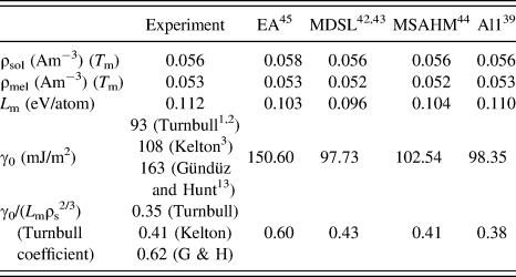
A comparison of crystal–melt interfacial free energy in Al with experiment and existing simulations including ours is given in Table III. Based on homogenous nucleation theory, TurnbullReference Turnbull1,Reference Turnbull and Cech2 obtained a value of 93 mJ/m2, and KeltonReference Kelton3 gave another value of 108 mJ/m2 from improved experiment later. However, from grain-boundary experiments, Gündüz and HuntReference Gündüz and Hunt13 provided a larger value of 163 mJ/m2. The result in our work is in good agreement with the nucleation data from the work of Turnbull and Kelton.Reference Turnbull1–Reference Kelton3 Although experiments from Gündüz and HuntReference Gündüz and Hunt13 benefitted from the fact that they did a more direct measurement, there were small amounts of Cu present in the materials, which not only directly affected the interfaces but also lowered the temperature at which the measurement carried out. As Morris et al.Reference Morris, Mendelev and Srolovitz30 argued, Cu would make the melt of Al more ordered, therefore influences the interfacial free energy strongly.
Calculated values related to melting and crystal–melt interfacial free energies. Previous simulation results are listed for comparison.

We also compared our work with Morris' results,Reference Morris, Mendelev and Srolovitz30 who computed the interfacial free energy in Al using CFM with three potentials. Our work gives results quite close to the MDSL potentialReference Mei and Davenport43,Reference Sturgeon and Laird44 and MSAHM potential,Reference Mendelev, Srolovitz, Ackland and Han45 but have large discrepancy with EA potential,Reference Ecolessi and Adams46 which are named by Morris et al.Reference Morris, Mendelev and Srolovitz30 For EA potentials, a set of crystal properties at room temperature were fitted, along with the forces obtained from the first-principle calculations on several model defects and melt structures. However, the pair correlation functions and structure factors of the melt predicted by this potential are more ordered than those from experimentReference Mendelev, Kramer, Becker and Asta39 such as x-ray diffraction. The crystal–melt interfacial free energy would be larger when melt structures appear more ordered (see Morris et al.Reference Morris, Mendelev and Srolovitz30). The Al1 potentialReference Mendelev, Kramer, Becker and Asta39 in our work as well as MSAHM potential comes from Mendelev, in which melt properties were used in the fitting procedure. After comparing with experiments, potential Al1 gives the melt structure more close to data from x-ray diffractions than MSAHM. Therefore, the interfacial free energy computed in our work gives results more close to the experiment from nucleation data. We also compared the Turnbull coefficients,Reference Turnbull1 which can be expressed as γ0/L mρs2/3 (L m is the latent heat of fusion and ρs is the number density of the crystal phase). Again the result in our work is in good agreement with the work from Turnbull and Kelton.
V. CONCLUSIONS
We have calculated the crystal–melt interfacial free energy of Al based on CFM with a transient LJ potential with a variable well depth to alter the force field of crystalline atoms. So stable crystal–melt interfaces were obtained and proper interface height fluctuation was ensured.Reference Morris, Wang, Ho and Chan36 We found that the dependence of the melting temperature on the orientation of interface: the interface with orientation (100)[001] corresponds to a lowest temperature, whereas (110) $\left[ {1\bar 10} \right]$ corresponds to the highest, and the average temperature of six orientations is 934.79 K, close to the data from experiment.Reference Smithels41 Using the stable crystal–melt interfaces, we calculated the average interfacial free energy (γ0: 98.35 mJ/m2) and the anisotropic parameters (ϵ1: 3.99%, ϵ2: −0.15%). We found that the average free energy is in good agreement with those obtained from nucleation dataReference Turnbull1–Reference Kelton3 and the anisotropy with an order of the values ranking as γ100 > γ110 > γ111, although the anisotropy of the interfacial free energy is weak.
ACKNOWLEDGMENTS
We would like to acknowledge the financial support to this work provided by the NSF of China (041303402) and National Magnetic Confinement Fusion Science program of China under Grant (2013GB109004, 2014GB117000). The work was carried out at National Supercomputer Center in Tianjin, and the calculations were performed on TianHe-1(A) and was also supported by Tsinghua National Laboratory for Information Science and Technology. M.L. acknowledges the support provided by the National Thousand Talents Program of China.
APPENDIX: ERROR ANALYSIS
According to Eq. (1), the interfacial stiffness γ̃ is related to the size of the capillary fluctuation modes, the later terms can be obtained from simulation directly. Therefore, the error of γ̃ comes from the distributions of capillary fluctuation modes <|A(k)|2 × k 2>, which can be expressed as
 $$A\left( k \right) = {a_k} + i{b_k}\quad .$$
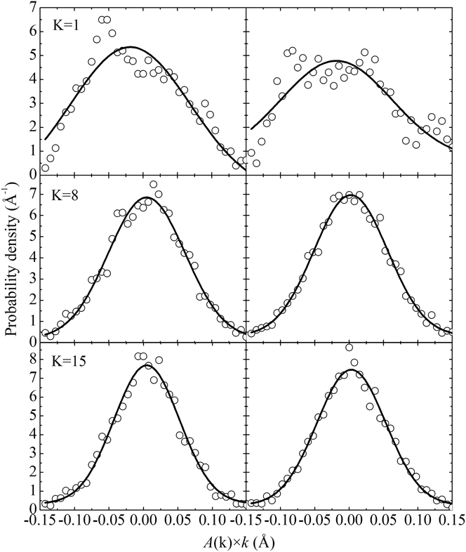
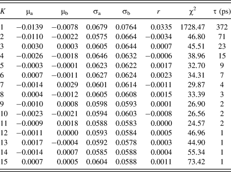
Figure 6 illustrated the distributions of |A(k)| × k for (100)[001] orientation, picked out from 4000 interface profiles for each simulation. We found that except for the longest mode (K = 1), both a k × k and b k × k tend to be Gaussian, and the correlation coefficient r is close to 0, the statistical data are shown in Table IV.
Distribution of interface fluctuation wave's amplitude. The left figure represents the real part of the amplitude whereas the right one represents the imaginary part. The solid lines are Gaussian.

Distribution of interface fluctuation wave's amplitude for (100)[001] orientations hypothesis testing.

We also conducted a Chi-square hypothesis testing for |A(k)| × k and found that most of the modes can be considered as 2D-Gaussian. In hypothesis testing, we used 6 × 6 inspection intervals, and the observations of samples χ2 are shown in Table IV. If significance level α was selected as 5%, the quantile of χ0.95(25) would be 37.652. It is found that for all modes except K = 1, |A(k)| × k follows 2D-Gaussian or similar distribution. This situation can be explained by different relaxation times, where the time correlation functionReference Hoyt, Trautt and Upmanyu42 can be expressed by
 $$\left\langle {A\left( {k,t} \right){A^*}\left( {k,0} \right)} \right\rangle = \left\langle {{{\left| {A\left( k \right)} \right|}^2}} \right\rangle \exp \left[ { - \mu \Gamma {k^2}t} \right]\quad ,$$
where μ is the kinetic coefficient and Γ = γ̃T M/L V, T M denotes the melting temperature and L V is the latent heat of fusion. Here, τ(t) is defined as
 $$\tau \left( t \right) = {{\left\langle {A\left( {k,t} \right){A^*}\left( {k,0} \right)} \right\rangle } \over {\left\langle {{{\left| {A\left( k \right)} \right|}^2}} \right\rangle }}\quad .$$
In Table IV, the relaxation times are given when τ = 0.1, the value can be considered as there is no relation between two interface profiles. For the longest mode (K = 1), this value is 372 ps, which is very large in simulation time, lead to dependence of |A(k)| × k. For the short mode, this independence becomes very weak and the distribution of |A(k)| × k tends to be 2D-Gaussian.
From Table IV, the averages of a k × k and b k × k (μa, μb) are close to 0, it is easy to be explained by fluctuation. The distributions of a k × k and b k × k are expressed below
 $${a_k} \times k{\;~\;}N\left( {0,\sigma _a^2} \right)\quad ,$$
 $${b_k} \times k{\;~\;}N\left( {0,\sigma _b^2} \right)\quad ,$$
where σa2 and σb2 denote the variance of a k × k and b k × k, respectively. From the statistics one can acquire
 $${1 \over {\sigma _a^2}}\mathop\sum\limits_{i = 1}^n {a_k^2 \times {k^2}{\;~\;}{\chi ^2}\left( n \right)} \to N\left( {n,2n} \right)\quad ,$$
 $${1 \over {\sigma _b^2}}\mathop\sum\limits_{i = 1}^n {b_k^2 \times {k^2}{\;~\;}{\chi ^2}\left( n \right)} \to N\left( {n,2n} \right)\quad ,$$
and the distribution of <|A(k)|2 × k 2> would be
 $$\left\langle {{{\left| {A\left( k \right)} \right|}^2} \times {k^2}} \right\rangle {\;~\;}N\left[ {\left( {\sigma _a^2 + \sigma _b^2} \right),{{2\left( {\sigma _a^4 + \sigma _b^4} \right)} \over n}} \right]\quad ,$$
where n is the number of samples, the value of 4000 in our work. From statistics, one can get the 95% confidence intervals of <|A(k)|2 × k 2> and γ̃(k) combining Eq. (1). Figure 7 shows the error bars of γ̃(k) for three orientations, by averaging the γ̃(k) at different k, the 95% confidence intervals of γ̃ can be acquired, as shown in Table II.
Error analysis of stiffness of different interface orientations, error bars indicate the 95% confidence intervals. The symbols used here are for different interfaces: ■ for (100)[001] interface, ● for (110)[001] interface, and ▲ for (111) $\left[ {1\bar 10} \right]$ interface.

Moreover, the distribution of |A(k)|2 × k 2 should follow Boltzmann distribution coming from the derivation of Eq. (1) as:
 $$p\left( {{{\left| {A\left( k \right)} \right|}^2} \times {k^2}} \right) = {{bL\tilde \gamma } \over {{k_{\rm{B}}}T}}\exp \left( { - {{\left| {A\left( k \right)} \right|}^2} \times {k^2} \times {{bL\tilde \gamma } \over {{k_{\rm{B}}}T}}} \right)\quad .$$
Indeed, a k × k and b k × k should obey the same distribution theoretically, with σa2 = σb2 = σ2. Therefore, the distribution of |A(k)|2 × k 2 would be written as:
 $${{{{\left| {A\left( k \right)} \right|}^2} \times {k^2}} \over {{\sigma ^2}}} \sim {\chi ^2}\left( 2 \right)\quad .$$
From Eq. (17), the probability density of |A(k)|2 × k 2 should be:
 $$p\left( {{{\left| {A\left( k \right)} \right|}^2} \times {k^2}} \right) = {1 \over {2{\sigma ^2}}}\exp \left( { - {{{{\left| {A\left( k \right)} \right|}^2} \times {k^2}} \over {2{\sigma ^2}}}} \right)\quad .$$
By comparison of Eq. (18) with Eq. (16), it can be found that 2σ2 = k BT/bLγ̃. At the same time, the distribution of <|A(k)|2 × k 2> would be written as:
 $$\left\langle {{{\left| {A\left( k \right)} \right|}^2} \times {k^2}} \right\rangle \,\sim\, N\left( {2{\sigma ^2},{{4{\sigma ^4}} \over n}} \right)\quad .$$
This equation illustrated the Gaussian distribution of <|A(k)|2 × k 2> in the case of σa2 = σb2, while the statistical data of these two parameters in our simulations are not necessarily the same (see Table IV). Consequently, we use Eq. (15) instead of (19) for error estimation.