Introduction
Through-the-wall radar imaging (TWRI) is a system that uses electromagnetic waves to detect and locate objects behind walls [Reference Nkwari, Sinha and Ferreira1]. In recent years, TWRI has gained increasing popularity in both military, search and rescue, and security applications [Reference Nkwari, Sinha and Ferreira1]. One of the several challenges that exist in TWRI is the development of through-the-wall imaging algorithm with unknown wall parameters for synthetic aperture radar (SAR) to generate three-dimensional (3D) images of the scene behind the wall [Reference Nkwari, Sinha and Ferreira1]. In practice, wall parameters are unknown or known with some degree of uncertainty. Using incorrect wall parameters during imaging can defocus the reconstructed image, leading to blurred or displaced target representations [Reference Kaushal, Kumar and Singh2].
Many autofocusing methods have been proposed for SAR to generate focused images when wall parameters are unknown. These methods can generally be grouped into three categories. The first category comprises trajectory-based approaches, which require two or more distinct array structures and are therefore time-consuming [Reference Wang, Wu, Qin and Hong3–Reference Xin, Biying, Pengfei and Zhimin7]. The second category involves estimating wall parameters prior to imaging [Reference Xu, Jin and Dai8–Reference Qu16]. In this case, unknown parameters can be retrieved through optimization techniques that minimize the mismatch between measured and predicted values, such as the reflection coefficient [Reference Solimene, Soldovieri, Prisco and Pierri9]. However, this process is often more complex than imaging itself and heavily depends on the accuracy of the modeling [Reference Wang, Wu, Qin and Hong3]. A simpler method for estimating the wall transmission coefficient has been introduced in Ref. [Reference Solimene, Di Napoli, Soldovieri and Pierri10], which avoids optimization but requires a multistatic configuration. In addition, direct estimation approaches that infer wall parameters directly from the reflected fields without optimization have also been reported [Reference Zhang, Wang, Wu, Wang and Zhang11–Reference Qu16]. The third category focuses on image quality optimization, which generally provides superior performance and has been widely adopted [Reference Xu, Jin and Dai8]. It is an iterative method that adjusts parameters based on a focus evaluation function until the image with the optimal focus is achieved [Reference Li, Zhang and Li17–Reference Akhter and Akhtar22]. Traditional imaging processing of the third kind of methods involves discretizing the defined search range for wall thickness and relative permittivity into equal intervals to generate all possible wall thickness and relative permittivity parameter pairs. For each pair, a radar image is formed and evaluated using a focusing metric. This process of image reconstruction and evaluation is performed for all parameter pairs. Then, the image corresponding to the pair with the best focusing metric is selected as the final focused image. Owing to this exhaustive image formation and evaluation process for all possible pairs, the imaging process described in Refs [Reference Li, Zhang and Li17–Reference Jin, Chen and Zhou20] poses a significant computational burden. To reduce the computational burden, some methods based on image domain filter and parametric sparse representation have been proposed [Reference Wang, Wu, Qin and Hong3, Reference Zhuo and Jin21, Reference Akhter and Akhtar22]. However, they still required a two-dimensional (2D) search over wall parameters, typically wall thickness and relative permittivity, which represents a large computational burden. Therefore, a more computationally efficient method is desirable.
This paper presents an efficient autofocusing method for the SAR-based 3D through-the-wall image formation, which will transform a 2D searching procedure into a one-dimensional (1D). Instead of adjusting both parameters, our method first estimates the wall’s relative permittivity using time-domain signals reflected from the front side of the wall. Then, it focuses on fine-tuning just one parameter, wall thickness, to create an optimal radar image. Thus, the proposed autofocusing method will transform a 2D searching procedure into a 1D problem. By reducing the process to a single adjustable parameter, our method is faster and uses fewer computational resources compared to traditional methods. This new approach is a major improvement because it simplifies the process while maintaining high image quality. It is especially useful for real-time radar systems, where quick and efficient imaging is essential. By narrowing the focus to one parameter and accurately estimating permittivity, our method is a practical and effective solution to the challenges of traditional autofocusing techniques. However, the effectiveness of the proposed method depends on an accurate initial estimate of  ${\varepsilon _r}$ and relies on modeling the wall as a single homogeneous layer, thereby limiting its applicability to thin or multilayered wall scenarios. The structure of the article is as follows: The “Proposed method” section describes the proposed novel real-time autofocusing algorithm, the “Experimental results” section presents simulation and experimental results to validate the method, while the “Conclusion” section presents the conclusion.
Proposed method
To efficiently address the 3D TWRI problem, a 2D slice-based imaging strategy is employed [Reference Solimene, Soldovieri, Prisco and Pierri9]. In this approach, data are acquired along a linear aperture parallel to the wall at multiple heights. For a given height, the measurements recorded as a function of antenna position and frequency form a B-scan dataset. Each B-scan is processed independently to reconstruct a 2D image slice corresponding to that height. A two-step imaging framework is proposed for through-the-wall scene reconstruction. In the first step, the wall thickness and dielectric permittivity are estimated from the B-scan data at a selected height using a simple and computationally efficient method. In the second step, 2D image slices are reconstructed at all heights. Finally, the 3D representation of the concealed scatterers is obtained by superimposing the individual 2D slices, resulting in a volumetric image of the scene.
In this section, we present the proposed two-stage autofocusing approach for 2D radar image formation from B-scan data. The main steps of the proposed method are shown in Fig. 1. The proposed method involves estimating the wall’s relative permittivity, followed by optimizing the 2D radar image by adjusting the wall thickness. The primary goal is to enhance image quality by iteratively refining the wall thickness based on estimated parameters. First, the value of the first peak  ${P_{t1}}$ coming from the first interface from the others will be separated to estimate the relative permittivity. In order to obtain a good estimation of relative permittivity, the signal should not take into account all the wall reflections but only the one coming from the first interface; otherwise, the relationship between relative permittivity and the reflection coefficient is more complicated and depends on the wall thickness. Next, an autofocusing method is used to obtain optimal 2D radar image by adjusting only the wall thickness parameter in each iteration, only the wall thickness is adjusted, and 2D radar images are generated using the updated wall thickness and estimated relative permittivity values. The image corresponding to this optimal thickness, achieved when the image quality parameter is maximized, is retained as the final output of the through-the-wall imaging result. Although there are several approaches for image formation, we employed delay and sum beamforming due to low computational load. This section first outlines the method for estimating the wall’s relative permittivity, followed by the autofocusing approach for image formation.
Flowchart of the proposed method.

Figure 1 Long description
The flowchart depicts a two-stage process for 2D radar image formation. It starts with acquiring S subscript n data at 27 by 21 horizontal and vertical scan points to obtain C-scan data. The first stage involves considering B-scan data at any height, labeled E subscript m (n, l). An inverse fast Fourier transform (IFFT) is applied, resulting in E subscript m (l). Background subtraction is performed to isolate the signal. Singular value decomposition (SVD) extracts the signal and the sum of E subscript m (n, l) is calculated to find the maximum value, estimating epsilon subscript r. The second stage repeats background subtraction and SVD to extract the target signal. A fast Fourier transform (FFT) is applied and the through-the-wall radar image (TWRI) is generated using delay and sum beamforming with estimated permittivity. The image quality is assessed for different thickness values, searching for the maximum quality parameter. The final output is the optimized through-the-wall radar image. The flowchart uses linear arrows to connect steps, indicating progression through the stages.
Stage 1: estimating the wall’s relative permittivity
Consider a stepped frequency continuous wave radar positioned at a standoff distance d from a wall, illuminating an infinitely long, homogeneous, smooth wall from a sufficient distance, as shown in Fig. 2. The radar transmits and receives the magnitude and phase of reflected signals over a frequency range from f min to f max across N frequency points at mth scan position. The received frequency domain data is then converted into the equivalent time domain using the standard inverse fast Fourier transform.
Through-the-wall image scene.

The antenna is placed in the far-field relative to the wall, ensuring that a transverse electromagnetic (TEM) wave is normally incident on the wall. When the wave impinges on the front surface, as shown in Fig. 2, a portion of the wave is reflected due to the permittivity discontinuity at the interface, while the remaining portion propagates into the wall. The backscattered signal from a single-layer homogeneous wall primarily consists of time-shifted and attenuated replicas of the transmitted pulse, with the first two dominant echoes arising from the front and rear wall interfaces. While real building materials are indeed inhomogeneous, prior studies have shown that when the characteristic size of inhomogeneities is smaller than the system’s pulse resolution, the wall can be accurately modeled as a homogeneous medium with an effective permittivity [Reference Protiva, Mrkvica and Machác23]. Under these conditions, the backscattered signal closely resembles that of an ideal homogeneous wall, and the dominant reflections still originate from the two interfaces, validating the underlying assumption used in our method. We also assume negligible material dispersion over the operating bandwidth, allowing the effective permittivity to be treated as frequency-independent. The first peak at time t 1 represents the received power  ${P_{t1}}$ of the wave reflected from the front surface of the wall. This formulation utilizes only the power quantity to determine the wall’s relative permittivity. The received power
 ${P_{t1}}\,$is a function of the reflection coefficient
 ${{\Gamma }}$ and the reference incident power
 ${P_{\text{i}}}$, as described by the following equations [Reference Akhter and Akhtar22]:
 \begin{equation}{P_{t1}} \cong {\left| {{\varGamma }} \right|^2}{P_{\text{i}}}\end{equation}
The magnitude of the reflection coefficient can be calculated using the following equation [Reference Akhter and Akhtar22]:
 \begin{equation}\left| {{\varGamma }} \right| \cong \sqrt {\frac{{{P_{t1}}}}{{{P_{\text{i}}}}}} \,\end{equation}
Once the magnitude of the local reflection coefficient is obtained, the relative permittivity of the wall  ${\varepsilon _r}\,$can be calculated using the following expression [Reference Akhter and Akhtar22]:
 \begin{equation}{{{\varepsilon }}_r} = {\left( {\frac{{1 + \left| {{\varGamma }} \right|}}{{1 - \left| {{\varGamma }} \right|}}} \right)^2}\end{equation}
In general, the reflection coefficient at a dielectric interface depends on both the relative permittivity  ${\varepsilon _r}\,$and the loss tangent
 $\tan \delta $. However, in this work, we adopt the standard assumption commonly used in TWRI studies that typical building materials are either lossless or only weakly lossy within the operating frequency band. As noted in Ref. [Reference Protiva, Mrkvica and Machác23], when the loss tangent is small, the propagation velocity is mainly governed by the real part of the permittivity, and the influence of the loss tangent becomes negligible. Consequently, under weak-loss conditions, the effect of
 $\tan \delta $ on both the phase and magnitude of the reflection coefficient is minor compared to the dominant contribution of
 ${\varepsilon _r}$. Therefore, within the low-loss approximation, the reflection coefficient can be treated primarily as a function of the permittivity.
The wall’s relative permittivity can be determined by exploiting  ${P_{t1}}$ at time point t 1 from the time-domain plot. The separation of the first echo from the reflections arising at subsequent interfaces is a critical step for accurately estimating the relative permittivity using Equation (3). Step 1 – Frequency to time domain conversion: The frequency domain data E(m, f) is converted into time-domain data E (m, t) by applying the inverse fourier transform. This gives the time-domain response at each scan point for all time values. Step 2 – Background subtraction: Background subtraction is applied to remove the antenna mismatch reflection from measured TWRI data.
 \begin{equation}E\!\left({m,t} \right) = E\!\left({m,t} \right) - {E_O}\!\left({m,t} \right),\end{equation}
where E(m, t) represents the measured time-domain data at the mth scan point and tth time instance, EO(m, t) represents the reference measurement performed in an anechoic chamber to account for antenna mismatch. This step ensures that the signal contains only the reflections due to the wall and targets. Step 3 – Singular value decomposition (SVD): SVD is performed to isolates the dominant wall reflection from other background components. Experimental findings in Ref. [Reference Tivive, Bouzerdoum and Amin24] demonstrate that SVD decomposes the time-domain data matrix into orthogonal singular vectors, where the dominant singular values correspond to the strongest reflections, typically from the wall, while the weaker singular values capture reflections from the target. When the wall and target echoes exhibit distinct temporal and spatial characteristics, they are mapped onto separate singular vectors, effectively ensuring their orthogonality. Wall reflections tend to be significantly stronger than target reflections due to the wall’s high reflectivity and larger surface area. This disparity in signal strength causes the wall subspace to dominate the leading singular values, whereas target echoes are represented in lower-energy singular components. A threshold can be set on the singular value spectrum to distinguish dominant components (associated with the wall) from non-dominant ones (representing the target and noise). Otsu’s method is commonly employed to identify the optimal threshold by maximizing the variance between these classes. For this, the time-domain data E(m, t) is decomposed using SVD into the wall subspace  ${E_W}\left( {m,t} \right)\,$and target subspace
 ${E_T}\left( {m,t} \right)$. The wall subspace component is selected based on Otsu’s method, which contains most of the wall reflection such that [Reference Tivive, Bouzerdoum and Amin24]
 \begin{equation}{E_W}\!\left({m,t} \right) = \sum\limits_{i \in W} {{\sigma _i}} {u_i}v_i^T,\end{equation}
where  ${\sigma _i}$ represent singular values arranged in decreasing order, i.e.
 ${{{\sigma }}_1} \gt {{{\sigma }}_2} \gt \ldots \gt {{{\sigma }}_N} \gt 0$,
 ${u_i}$ and
 ${v_i}$ represent left and right singular vectors. Step 4 – Finding
 ${P_{t1}}$ and relative permittivity: First,
 ${S_W}\!\left({m,t} \right)$ are added up in the time domain given as
 \begin{equation}\sum\!\left(t \right) = \mathop \sum \limits_{m = 1}^M \left| {{E_W}\!\left( {m,t} \right)} \right|\end{equation}
Next, find the index value t 1 at which the sum is maximum, which corresponds to the time when the first echo is most pronounced in time domain profile. Then, find  ${P_{t1}}$ at time points t 1 from time-domain profile of any one scan point, say m = 10.
 \begin{equation}{\text{ }}\,{P_{t1}} = E\!\left( {m = 10,{t_1}} \right)\end{equation}
Stage 2: autofocusing method is employed to generate a focused image
Once the relative permittivity is estimated, time-domain data  ${E_T}\!\left( {m,t} \right) = \mathop \sum \limits_{i \in T} {\sigma _i}{u_i}v_i^T$ representing the target subspace converted can be converted to the frequency domain. The delay and sum beamforming algorithm can be applied to frequency domain data. Using the estimated relative permittivity, an image quality optimization scheme can be applied to recursively autofocus the images. In each iteration, the assumed wall thickness value is modified, and a new beamformed image is generated based on the updated wall thickness. According to the delay and sum beamforming imaging algorithm, the value for the (x, y) pixel (x = 1, 2, …, Nx; y = 1, 2, …, Ny) is determined by [Reference Tivive, Bouzerdoum and Amin24]
 \begin{equation}I\!\left( {x,y} \right) = \frac{1}{{MN}}\mathop \sum \limits_{m = 1}^M \mathop \sum \limits_{n = 1}^N {k_{m,n}}\exp \!\left( {j2\pi {f_n}{\tau _m}\left( {x,y} \right)} \right)\end{equation}
Here,  ${\tau _m}\left( {x,y} \right)$ represents the focusing delay between the mth scan point and the target situated at the pixel position (x, y). This focusing delay can be calculated using Snell’s law, along with the distance from the transceiver to the front wall and the distance from the target to the back wall (see Ref. [Reference Akhter and Akhtar22]). The signal received at the mth antenna location and the nth frequency, denoted as
 ${z_{m,n}}$, is given by [Reference Tivive, Bouzerdoum and Amin24]
 \begin{equation}{k_{m,n}} = \mathop \sum \limits_{r = 1}^R {{{\sigma }}_r}\!\left( {{f_n}} \right)\exp\!\left( { - j2{{\pi }}{f_n}{{{\tau }}_{m,r}}} \right)\end{equation}
 ${\sigma _r}\!\left( {{f_n}} \right)\,$represents the reflection coefficient of the rth target at the nth frequency, while
 $\,{{{\tau }}_{m,r}}$ denotes the round-trip travel time of the signal from the mth antenna location to the rth target location. It is well established that using an incorrect wall thickness value for imaging leads to decreased image resolution and causes the target to shift from its true position [Reference Kaushal, Kumar and Singh2], resulting in reduced contrast in the resulting image. To obtain the optimal thickness value and the corresponding image, we use a well-known metric to measure the quality of a focused image, which is the higher-order moment of the image and is given by
 \begin{equation}M = \frac{1}{n}\mathop \sum \limits_{i = 1}^n {\left( {{x_i} - \bar x} \right)^5}\,\end{equation}
where n represents the no. of pixels, m is the order of the moment,  ${x_i}$ is the ith data value, and
 $\bar x$ is the mean of the data values. The optimal thickness can then be determined by identifying the maximum value of the moment. The image corresponding to this optimal thickness value, where the moment in Eq. (10) is maximized, is saved as the output of the 2D radar image results.
Experimental results
In this section, the proposed method for 2D image formation is first validated using synthetic data. The B-scan dataset was generated for a monostatic SAR system positioned at a standoff distance of 1 m from the wall and operating at a center frequency of 4.5 GHz with a bandwidth of 2 GHz and a frequency step of 10 MHz. Electromagnetic simulations were carried out using CST Microwave Studio. The antenna was scanned horizontally from −0.65 m to 0.65 m with a step size of 0.05 m. Two different TWRI scenarios were considered.
In Scene 1, the wall had a relative permittivity of ɛ r = 2.5 and a thickness of 0.10 m, whereas in Scene 2, the wall permittivity was relative permittivity ɛ r = 6.5 and a thickness of 0.30 m. In both cases, two targets were located behind the wall at positions (0.25, 1.42 m) and (−0.25, 2.17 m). The reconstruction process began with the estimation of the wall’s relative permittivity, followed by an iterative autofocusing procedure in which the wall thickness was treated as the optimization parameter.
Using Steps 1–4, the first reflected wall peak  ${P_{t1}}$ for both scenes was identified at the time instant t 1. B-scan data were transformed to the time domain, and background subtraction was performed using Steps 1 and 2. In Step 3, the time-domain data were decomposed into wall and target subspace components. Step 4 was then applied to compute Sum(t) from the wall subspace and determine t 1 by locating the time at which Sum(t) reached its maximum. In Step 5,
 ${P_{t1}}$ was obtained as
 ${P_{t1}}$ = S(m, t 1), and the wall’s relative permittivity was subsequently estimated.
With the estimated permittivity, image reconstructions were carried out using 14 scan positions and 101 frequency bins while varying the wall thickness from 0.05 to 0.35 m in steps of 0.01 m. For each assumed thickness, the moment value was computed, and the image corresponding to the maximum moment value was selected as the optimally focused result. The reconstructed images for different wall thicknesses in Scenes 1 and 2 are shown in Figs 3(a) and 4(a), respectively. For Scene 1, the maximum moment occurred at the true wall thickness of 0.10 m, while for Scene 2 it was observed at 0.30 m. Reconstructions obtained using incorrect thickness values, shown in Figs 3(b–c) and 4(b–c), exhibit noticeable defocusing and smearing compared to the sharply focused images obtained at the correct wall thickness.
Reconstruction results at different thickness values (d) for Scene 1.

Figure 3 Long description
The image A showing a heatmap with Crossrange(in meter) on the vertical axis and Downrange(in meter) on the horizontal axis. The right-side scale bar is labeled (dB) with tick labels 0, minus 1, minus 3, minus 6, minus 48. Higher values are at 0 and lower values are toward minus 48. A small, strongest-intensity patch appears near Downrange about 1.5 and Crossrange about 0.25. A smaller patch appears near Downrange about 2.2 and Crossrange about minus 0.25. The image B showing a heatmap with Crossrange(in meter) on the vertical axis and Downrange(in meter) on the horizontal axis. The right-side scale bar is labeled (dB) with tick labels 0, minus 1, minus 3, minus 6, minus 40. Higher values are at 0 and lower values are toward minus 40. A strongest-intensity patch appears near Downrange about 1.4 and Crossrange about 0.25, with a short horizontal spread to the right. Another smaller patch appears near Downrange about 2.2 and Crossrange about minus 0.25. The image C showing a heatmap with Crossrange(in meter) on the vertical axis and Downrange(in meter) on the horizontal axis. The right-side scale bar is labeled (dB) with tick labels 0, minus 1, minus 3, minus 6, minus 39. Higher values are at 0 and lower values are toward minus 39. A strongest-intensity patch appears near Downrange about 1.4 and Crossrange about 0.25. Another smaller patch appears near Downrange about 2.2 and Crossrange about minus 0.25. Compared across A, B and C, the strongest-intensity patch stays near Downrange about 1.4 to 1.5 and Crossrange about 0.25 and the smaller patch stays near Downrange about 2.2 and Crossrange about minus 0.25.
The results presented in Figs 4(a) and 5(a) were generated using noise-free data. To assess the robustness of the proposed approach, 20% additive random noise was introduced into the simulated dataset. The corresponding reconstructions, shown in Figs. 5(a) and 5(b), remain comparable to the noise-free case. Moreover, the moment curves plotted over different wall thickness values in Figs. 5(c) and 5(d) display similar trends under varying noise conditions, with the maximum moment consistently occurring at the true wall thickness for both scenes, thereby demonstrating the strong noise robustness of the proposed algorithm.
Reconstruction results at different thickness values (d) for Scene 2.

Figure 4 Long description
The image A showing a heatmap with the horizontal axis labeled Downrange(in meter) and tick labels 0, 0.5, 1, 1.5, 2, 2.5, 3, 3.5, 4, 4.5. The vertical axis is labeled Crossrange(in meter) with tick labels 0.6, 0.4, 0.2, 0, minus 0.2, minus 0.4, minus 0.6. A vertical color scale is labeled (dB) with tick labels 0, minus 1, minus 3, minus 6, minus 48. Two compact high-value regions are visible: one near downrange about 1.5 and crossrange about 0.2 to 0.3 and one near downrange about 2.2 and crossrange about minus 0.2 to minus 0.3. Each compact region aligns with a narrow vertical streak at the same downrange position. The text under the heatmap reads (a) d=0.30 m. The image B showing a heatmap with the horizontal axis labeled Downrange(in meter) and tick labels 0, 0.5, 1, 1.5, 2, 2.5, 3, 3.5, 4, 4.5. The vertical axis is labeled Crossrange(in meter) with tick labels 0.6, 0.4, 0.2, 0, minus 0.2, minus 0.4, minus 0.6. A vertical color scale is labeled (dB) with tick labels 0, minus 1, minus 3, minus 6, minus 42. Two compact high-value regions are visible: one near downrange about 1.7 and crossrange about 0.2 to 0.3 and one near downrange about 2.5 and crossrange about minus 0.2 to minus 0.3. Each compact region aligns with a narrow vertical streak at the same downrange position. The text under the heatmap reads (b) d=0.11 m. The image C showing a heatmap with the horizontal axis labeled Downrange(in meter) and tick labels 0, 0.5, 1, 1.5, 2, 2.5, 3, 3.5, 4, 4.5. The vertical axis is labeled Crossrange(in meter) with tick labels 0.6, 0.4, 0.2, 0, minus 0.2, minus 0.4, minus 0.6. A vertical color scale is labeled (dB) with tick labels 0, minus 1, minus 3, minus 6, minus 41. Two compact high-value regions are visible: one near downrange about 1.5 and crossrange about 0.2 to 0.3 and one near downrange about 2.2 to 2.3 and crossrange about minus 0.2 to minus 0.3. Multiple faint vertical streaks are visible at additional downrange positions across the heatmap area. The text under the heatmap reads (c) d=0.27 m.
(a) Reconstruction results with 20% noise of Scene 1, (b) Reconstruction results with 20% noise of Scene 2, (c) Moment value plots with and without noise in the case of Scene 1, and (d) Moment value plots with and without noise in the case of Scene 2.

Figure 5 Long description
The image A showing a heatmap with the horizontal axis labeled Downrange(meter) and tick labels 0, 0.5, 1, 1.5, 2, 2.5, 3, 3.5, 4, 4.5. The vertical axis is labeled Crossrange(meter) with tick labels negative 0.6, negative 0.4, negative 0.2, 0, 0.2, 0.4, 0.6. A vertical color scale bar is shown at the right with tick labels negative 45, negative 40, negative 35, negative 30, negative 25, negative 20, negative 15, negative 10, negative 5, 0. The image B showing a heatmap with the horizontal axis labeled Downrange(meter) and tick labels 0, 0.5, 1, 1.5, 2, 2.5, 3, 3.5, 4, 4.5. The vertical axis is labeled Crossrange(meter) with tick labels negative 0.6, negative 0.4, negative 0.2, 0, 0.2, 0.4, 0.6. A vertical color scale bar is shown at the right with tick labels negative 45, negative 40, negative 35, negative 30, negative 25, negative 20, negative 15, negative 10, negative 5, 0. The image C showing a line graph with the horizontal axis labeled Wall thickness(meter) and tick labels 0, 0.1, 0.2, 0.3, 0.4. The vertical axis is labeled Value of moment with a scale note times 10 superscript negative 15 and tick labels 0, 0.5, 1, 1.5, 2, 2.5. A legend shows Noise Free and 20 percent Random Noise. The plotted points for both series follow the same visible curve with two main peaks near wall thickness 0.1 and 0.2 and a smaller rise near 0.35. The image D showing a line graph with the horizontal axis labeled Wall thickness(meter) and tick labels 0, 0.1, 0.2, 0.3, 0.4. The vertical axis is labeled Value of moment with a scale note times 10 superscript negative 15 and tick labels 0, 2, 4, 6. A legend shows Noise Free and 20 percent Random Noise. Multiple peaks and troughs are plotted across the wall thickness range, with repeated sharp peaks near the top tick value 6 and several low points near the baseline between peaks.
To evaluate the effectiveness of the proposed method, the proposed method was tested with real B-scan data obtained through an experiment. The experiment utilized SFCW radar, and the actual measurement system, as shown in Fig. 2, consisted of a horn antenna, a vector network analyzer, and a field scanner. A real building wall made up of bricks and covered by fine layer of plaster with a known thickness of 0.145 m and measured relative permittivity of 4.1 was examined. The radar was positioned 2.2 m away from the front side of the wall. Two TWRI scenarios were created and the target combinations are placed behind the wall: (i) In first scenario, a single metallic target with a very high dielectric constant was placed behind the wall. (ii) While in the second scenario, a combination of targets was used to create a contrast in dielectric properties. One target was wood, with a very low dielectric constant, while the other was metallic, with a much higher dielectric constant. Photographs of the targets and their measured radar cross-section (RCS) values are presented in Table 1. The RCS measurements for objects, such as metallic and wooden plates, were conducted using a step-frequency RCS measurement system. This system includes a network analyzer that transmits and receives step-frequency signals, a horn antenna for transmission and reception, high-performance absorbers in an anechoic chamber, and low scattering rigid supports made of low-density foam. The RCS measurement of targets using a quasi-monostatic configuration has been done as per the method described in Ref. [Reference Hu, Xu, Li and Zhang25].
Detail of targets behind the wall

Table 1 Long description
The table lists targets used in a TWRI scenario, giving each target’s identifier and size, its radar cross section value in dBsm, and its distance from the wall in meters. Scenario 1 uses a metal target labeled T1Metal, sized 30 cm by 30 cm, with an RCS of 7.4 at 1.2 m from the wall. Scenario 2 uses a wood target labeled T2Wood, also 30 cm by 30 cm, with an RCS of minus 6.8 at 2.8 m from the wall. A third entry repeats the metal target T1Metal with the same RCS of 7.4 but placed closer, at 0.6 m from the wall. Across the listed entries, the metal target’s RCS is much higher than the wood target’s. The repeated metal entry suggests the RCS value is treated as unchanged even when the distance from the wall differs, so the table does not indicate how distance affects RCS.
The data are collected using a stepped-frequency radar system operating within a frequency range of 3.5–5.5 GHz, with a frequency step size of 10 MHz [Reference Gaikwad, Singh and Nigam26]. This results in 201 frequency bins (N = 201). The scene is illuminated by an antenna as it moves horizontally across 27 scan positions (M = 27). The full data set, therefore, contains M × N, or 27 × 201, which equals 5427 samples. The scattering parameter S 11 was measured using the VNA across 201 frequency points within the range of 3.5–5.5 GHz at 27 scan points along the horizontal direction. The wall is in the far-field region, allowing the assumption that the TEM wave is incident normally on the wall. The frequency domain data acquired is converted into the time domain to exploit the  ${P_{t1}}$ and estimate the relative permittivity value using Steps 1–4. The inverse Fourier transform converts frequency-domain data E(m, f) into time-domain data, yielding the time response at each scan point. To remove antenna mismatch reflections, a reference signal EO(m, t) from an anechoic chamber is subtracted, leaving only reflections from the wall and targets. SVD was applied to separate the wall and target echoes. To obtain
 ${P_{t1}}$ at time point t 1 for all scan points,
 ${E_W}\left( {m,t} \right)$ is summed in the time domain, the index t 1 corresponding to the maximum sum is identified, and
 ${P_{t1}}$ at t 1 is determined from the time-domain profile for a selected scan point m = 10. From
 ${P_{t1}},$ the relative permittivity value of wall was estimated which was found to be 4.3. The results corresponding to Steps 1–4 are presented in Fig. 6(a–f).
(a) Raw B-scan image of Scene 1 in time domain after Step 1, (b) Raw B-scan image of Scene 2 in time domain after Step 1, (c) B-scan image after application of background subtraction and SVD on Scene 1 using Steps 2 and 3, (d) B-scan image after application of background subtraction and SVD on Scene 2 using Steps 2 and 3, (e) Plot of sum after Step 4 of Scene 1, (f) Plot of sum after Step 4 of Scene 2.

Figure 6 Long description
The image A showing a heatmap with the y-axis labeled Scan positions, ranging from 0 to 25. The x-axis is labeled Time(seconds), ranging from 0 to 2.5 times 10 superscript minus 8. Text labels inside the plot read Antenna Mismatch, Wall Reflections and Target Reflections. The image B showing a heatmap with the y-axis labeled Scan positions, ranging from 0 to 25. The x-axis is labeled Time(seconds), ranging from 0 to 2.5 times 10 superscript minus 8. Text labels inside the plot read Antenna Mismatch, Wall Reflections, Target1 Reflection and Target2 Reflection. The image C showing a heatmap with the y-axis labeled Scan positions, ranging from 0 to 25. The x-axis is labeled Time(seconds), ranging from 0 to 2.5 times 10 superscript minus 8. A text label inside the plot reads Wall Reflection. The image D showing a heatmap with the y-axis labeled Scan positions, ranging from 0 to 25. The x-axis is labeled Time(seconds), ranging from 0 to 2.5 times 10 superscript minus 8. A text label inside the plot reads Wall Reflections. The image E showing a line plot with the y-axis labeled Sum, ranging from 0 to 0.4. The x-axis is labeled Time(seconds), ranging from 0 to 2.5 times 10 superscript minus 8. A text label points to the tallest peak and reads Front Wall Peak. The curve rises to a sharp maximum near 0.5 times 10 superscript minus 8, then drops and shows smaller peaks around about 0.7 times 10 superscript minus 8, about 1.6 times 10 superscript minus 8 and about 1.9 times 10 superscript minus 8. The image F showing a line plot with the y-axis labeled Sum, ranging from 0 to 0.4. The x-axis is labeled Time(seconds), ranging from 0 to 2.5 times 10 superscript minus 8. A text label points to the tallest peak and reads Front Wall Peak. The curve rises to a sharp maximum near 0.5 times 10 superscript minus 8, then drops and shows smaller peaks around about 0.65 times 10 superscript minus 8, about 1.6 times 10 superscript minus 8 and about 1.9 times 10 superscript minus 8.
Using the estimated relative permittivity, an image quality optimization scheme can be applied iteratively to achieve autofocus in the images. In each iteration, the assumed wall thickness value is modified, and a new beamformed image is generated based on the updated wall thickness. The thickness varies from 0.10 to 0.20 m. The optimal thickness value is determined at the moment when the moment value of the image reaches its maximum, and the corresponding image represents the final imaging result. Figure 7(a) and 7(c) displays the moment values at different thicknesses of Scenes 1 and 2. From the Fig. 7(a) and 7(c), it is clear that the value of the moment is maximum at the wall thickness of 0.15 m.
(a) Moment value at different thickness value for single target scene, (b) Reconstructed results with autofocusing for single target scene when the wall thickness is estimated as d = 0.15 m, (c) Moment value at different thickness value for contrast target scenario, (d) Reconstructed results with autofocusing for two target scenarios when the wall thickness is estimated as d = 0.15, (e) Reconstructed results with true wall parameter values for Scene 1, (f) Reconstructed results with true wall parameter for Scene 2.

Figure 7 Long description
The image A showing a line graph with a legend listing six series labeled mod 1, mod 2, mod 3, mod 4, mod 5 and mod 6. The x-axis is labeled Wall Thickness (in meter), ranging from 0.10 to 0.20. The y-axis is labeled Moment, ranging from 0 to 1.2. Each series forms a broad peak near wall thickness 0.15 and lower values near 0.10 and 0.20. Callout labels mark values near the peak for each series. The image B showing a heatmap. The x-axis is labeled Downrange (in meter), ranging from 0 to 5. The y-axis is labeled Crossrange (in meter), ranging from minus 0.6 to 0.6. A vertical color scale at the right is labeled (in decibel), with tick labels 0, minus 1, minus 2, minus 3 and minus 4. A circled region near downrange about 1.2 and crossrange about 0 is annotated with the word Target. The image C showing a line graph with a legend listing six series labeled mod 1, mod 2, mod 3, mod 4, mod 5 and mod 6. The x-axis is labeled Wall Thickness (in meter), ranging from 0.10 to 0.20. The y-axis is labeled Moment, ranging from 0 to 2.5. Each series rises to a peak near wall thickness 0.15 and decreases toward 0.10 and 0.20. Callout labels mark values near the peak for each series. The image D showing a heatmap. The x-axis is labeled Downrange (in meter), ranging from 0 to 5. The y-axis is labeled Crossrange (in meter), ranging from minus 0.6 to 0.6. A vertical color scale at the right is labeled (in decibel), with tick labels 0, minus 1, minus 2, minus 3 and minus 4. Bright vertical features appear near downrange about 0.6 and about 3.0. The image E showing a heatmap. The x-axis is labeled Downrange (in meter), ranging from 0 to 5. The y-axis is labeled Crossrange (in meter), ranging from minus 0.6 to 0.6. A vertical color scale at the right is labeled (in decibel), with tick labels 0, minus 1, minus 2, minus 3 and minus 4. A bright vertical feature appears near downrange about 0.7 and another weaker vertical feature appears near downrange about 4.0. The image F showing a heatmap. The x-axis is labeled Downrange (in meter), ranging from 0 to 5. The y-axis is labeled Crossrange (in meter), ranging from minus 0.6 to 0.6. A vertical color scale at the right is labeled (in decibel), with tick labels 0, minus 1, minus 2, minus 3 and minus 4. Bright vertical features appear near downrange about 0.6 and about 3.0.
Figure 7(b) and 7(d) shows the reconstructed results with autofocusing of Scenes 1 and 2 when the thickness parameter is estimated as d = 0.15 m. Reconstructed results for Scene 1 and Scene 2, respectively, when the wall parameters are correctly known, are also shown in Fig. 7(e) and 7(f). It can be observed that the reconstructed images shown in Fig. 7(b) and 7(d) closely resembles with Fig. 7(e) and 7(f) demonstrate accurate target localization with well-focused images, confirming the effectiveness of the proposed algorithm. Thus, the proposed algorithm can yield high-quality focused imaging results. This simulation was conducted on a personal computer equipped with an Intel Core i7 processor and 16 GB of RAM in a MATLAB environment.
In addition, reconstruction results corresponding to incorrect relative permittivity and wall thickness values are also presented. Figure 8(a) shows the reconstruction obtained when the relative permittivity is incorrectly estimated as 6.5, with the maximum moment occurring at a thickness of 0.195 m. Consequently, the target is shifted from its true location in the radar image. Figure 8(b) and 8(c) presents the reconstructed images for Scene 2 at wall thickness values different from the true value, resulting in blurred and defocused images. It can be observed that using incorrect wall parameters during imaging can defocus the reconstructed image, leading to blurred or displaced target representations.
(a) Reconstructed results with autofocusing for single target scene when ɛ r = 2.7 and d = 0.11 m, (b) Reconstructed result at thickness value = 0.12 m for Scene 2, (c) Reconstructed result at thickness value = 0.19 m for Scene 2.

Figure 8 Long description
Three heatmaps display reconstructed results with autofocusing for a single target scene. The vertical axis is labeled ‘Crossrange(in meter)’ and the horizontal axis ‘Downrange(in meter)’. Each heatmap includes a decibel scale indicating intensity, with higher values representing stronger returns. In image A, the decibel scale ranges from 0 to minus 34, with a peak intensity around Downrange 1 meter and Crossrange 0.2 meter. Image B, with a thickness value of 0.12 meter, shows a decibel range from 0 to minus 32, with peaks near Downrange 0.5 meter and Crossrange 0.2 meter. Image C, at a thickness of 0.19 meter, has a decibel range from 0 to minus 33, with intensity peaks around Downrange 0.5 meter and Crossrange 0.2 meter. The heatmaps illustrate how variations in thickness affect the reconstructed intensity patterns.
To further demonstrate the effectiveness of the proposed approach for 3D image reconstruction, experimental results are presented in this section. Using the same measurement setup, B-scan data were acquired at 21 different heights. The target T1 was positioned at a distance of 1.22 m behind the wall. In the first stage, the wall thickness and dielectric permittivity were estimated from the B-scan data at a selected height using the proposed autofocusing procedure. In the second stage, the estimated wall parameters were used to reconstruct 2D image slices at all heights. The measured data were first converted to the time domain, and background subtraction was performed following Steps 1 and 2. Step 3 was then applied to decompose the time-domain data into wall and target subspace components. In Step 4, Sum(t) was computed from the wall subspace, and the time instant t 1 corresponding to its maximum was identified. The results of Steps 1–4 are illustrated in Fig. 9(a–c).
(a) Raw B-scan image after converting to time domain using Step 1, (b) B-scan image having wall reflections after applying Steps 2 and 3, (c) Sum of all A-scans along downrange Sum(t), (e) Autofocused 2D slice radar image corresponding to the maximum moment value.

Figure 9 Long description
The image A showing a heatmap with the vertical axis labeled Crossrange (meters) and the horizontal axis labeled Time (seconds). The time axis runs from 0 to 5 with a multiplier of 10 superscript minus 8. The crossrange axis runs from minus 0.5 to 0.5. The heatmap contains mostly low-intensity background with faint vertical streaks. The image B showing a heatmap with the vertical axis labeled Crossrange (meters) and the horizontal axis labeled Time (seconds). The time axis runs from 0 to 5 with a multiplier of 10 superscript minus 8. The crossrange axis runs from minus 0.5 to 0.5. A bright vertical band appears near time about 1.0 times 10 superscript minus 8, spanning most of the crossrange range. Additional weaker vertical streaks appear at later times. The image C showing a line graph with the vertical axis labeled Sum(t) and the horizontal axis labeled Time (seconds). The time axis runs from 0 to 5 with a multiplier of 10 superscript minus 8. The curve has a dominant peak near time about 1.0 times 10 superscript minus 8, annotated with the text Front Wall Peak. Several smaller peaks follow between about 1.2 and 2.5 times 10 superscript minus 8 and the curve then stays near a low level with small fluctuations through 5 times 10 superscript minus 8. The image D showing a heatmap with the vertical axis labeled Crossrange (meters) and the horizontal axis labeled Downrange (meters). The downrange axis runs from 0 to 5. The crossrange axis runs from minus 0.5 to 0.5. A vertical oval outline encloses a bright region near downrange about 1.0 and crossrange near 0, with the nearby text Target. Other weaker bright patches appear at larger downrange values. A vertical color scale bar is shown at the right with numeric labels 0 at the top and 34 at the bottom.
Finally, in Step 5, the first wall reflection peak  ${P_{t1}}$ was obtained as
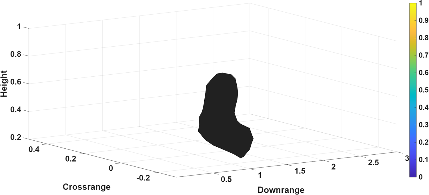
 ${P_{t1}}$ = S(m, t 1), and the wall’s relative permittivity was estimated accordingly. Using the estimated permittivity, 2D slice radar images of size (27 × 67) pixels were reconstructed for wall thickness values ranging from 0.10 to 0.20 m, and the moment value was computed for each case. The optimal wall thickness was identified at the point where the moment value reached its maximum, and the corresponding image was selected as the final focused result. Figure 9(d) shows the autofocused 2D slice radar image corresponding to the maximum moment value. With the estimated wall parameters, all 2D slice reconstructions were combined to form a 3D representation of the concealed scatterers by superimposing the individual slices, yielding a volumetric image of the scene. The reconstructed 3D radar image result is shown in Fig. 10.
Reconstructed 3D radar image of the scene by superimposing the individual 2D radar image slices at different heights.

Comparison with other image quality-based autofocusing methods
The proposed method is compared with existing image quality-based autofocusing methods as shown in Table 2 in terms of computational cost, wall parameter search range, accuracy and reliability. The computational cost in Refs [Reference Kaushal, Kumar and Singh2] and [Reference Xu, Jin and Dai8] is expressed as O(Nε r · Nd · Nx · Ny · Nz) + O(Nε r · Nd), because for each combination of relative permittivity ( ${{{\varepsilon }}_r}$) and wall thickness (d), the algorithm reconstructs an image over all pixel points (Nx × Ny × Nz), and computes a focusing metric once per (
 ${{{\varepsilon }}_r}$, d) pair. The term O(Nε r · Nd) appears because for each combination of relative permittivity (
 ${{{\varepsilon }}_r}$) and wall thickness (d), a total of Nε × Nd pairs, the algorithm evaluates a focus metric (e.g., entropy, sparsity, contrast), which typically returns a single scalar value used to identify the best (
 ${{{\varepsilon }}_r}$, d) combination. The computational cost of the proposed method is O(Nd · Nx · Ny) + O(Nd) is calculated by reconstructing images over all pixel points (Nx × Ny) for each wall thickness value (d), assuming
 ${{{\varepsilon }}_r}$ is known, and performing a focus metric evaluation once per thickness value, contributing the additional O(Nd) term. The computational cost is highest for O(Nε r · Nd · Nx · Ny · Nz) + O(Nε r · Nd), where both
 ${{{\varepsilon }}_r}$ and d are unknown and image reconstruction and focus metric evaluation are performed for every (
 ${{{\varepsilon }}_r}$, d) pair and it is lowest for O(Nd · Nx · Ny) + O(Nd) when
 ${{{\varepsilon }}_r}$ is known, requiring reconstruction and evaluation only across different wall thickness values.
Comparison of proposed method with other image quality-based autofocusing methods

Table 2 Long description
The table compares computational cost growth for three autofocusing approaches. References 2 and 8 have the same cost pattern: they scale with the number of tested wall permittivity values and wall thickness values, multiplied by the number of image points in the horizontal, downrange, and vertical directions, plus an added term that scales with permittivity and thickness only. The proposed method scales with the number of tested wall thickness values multiplied by the number of image points in the horizontal and vertical directions, plus an added term that scales with thickness only. Compared with references 2 and 8, the proposed method avoids dependence on the number of permittivity values and does not include the downrange image dimension in its main scaling term. This indicates the proposed method should require fewer computations as the search over wall properties or the downrange image size increases. The table reports asymptotic scaling only, so constant factors and implementation details are not reflected.
Nε r = The number of values considered for relative permittivity ( ${{{\varepsilon }}_r}$) of the wall, Nd = The number of values considered for wall thickness (d), Nx = The number of pixel points (or image points) in the x direction (horizontal), Ny = The number of pixel points (or image points) in the y direction (downrange), Nz = The number of pixel points (or image points) in the z direction (vertical).
Limitations and future work
The proposed autofocusing method optimizes only wall thickness (d), reducing computational complexity for real-time radar applications. It enhances accuracy by estimating relative permittivity from time-domain reflections, minimizing errors from incorrect wall assumptions. The method improves feasibility with fewer iterations and single-variable optimization, making it ideal for security and search-and-rescue operations. It integrates seamlessly into TWRI systems without extra wall measurements. However, its effectiveness depends on an accurate initial  ${\varepsilon _r}$ estimate and remains untested in highly cluttered or dynamic environments. Moreover, the proposed method assumes that the wall can be modeled as a single homogeneous layer by clearly separating the front-wall and rear-wall echoes. This assumption is valid only when the wall is not electrically thin. In practice, the wall thickness must satisfy
 $d \gt \frac{c}{{2\left( {{f_{max}} - {f_{min}}} \right)\sqrt {{\varepsilon _r}} }}$ to ensure reliable operation. Walls with thicknesses below this minimum limit violate the underlying assumption, which may degrade reconstruction accuracy. Additionally, it may not be suitable for multilayered walls, limiting its applicability in complex scenarios. Accurate wall parameter estimation is essential for optimizing transceiver placement and enhancing target resolution in TWRI systems [Reference Maisto, Masoodi, Pierri and Solimene27, Reference Maisto, Masoodi and Solimene28]. Future work will focus on developing a quantitative metric that integrates localization accuracy, spatial resolution, and contrast enhancement for a comprehensive assessment of imaging performance.
Conclusion
This paper presents an image autofocusing method for SAR-based 3D TWRI system. The approach begins by estimating the wall’s relative permittivity from measurements. Using the estimated relative permittivity, it generates an autofocus image by adjusting only the wall thickness parameter. This method utilizes a single search variable, thereby minimizing the computational load on a real-time radar system. An experiment was conducted to evaluate the effectiveness of the proposed method. The experimental results confirm that the method successfully produces well-focused images, demonstrating its applicability in addressing the complexities related to real building walls.
Competing interests
The authors declare none.

Dr Akhilendra Pratap Singh received the PhD degree in Electronics Engineering from the Indian Institute of Technology (BHU), Varanasi, India. He is presently serving as an assistant professor in the Department of Electronics and Communication Engineering at Indian Institute of Information Technology Bhopal. His research interests include radar signal and image processing. He has published various research articles in reputed international journals and conferences.

Dr Vineet Singh received the PhD degree in Electronics Engineering from the Indian Institute of Technology (BHU), Varanasi, India. He is currently an assistant professor in the Department of Electronics and Communication Engineering at the National Institute of Technology (NIT), Patna. Prior to this, he was a Postdoctoral Research Associate at the Indian Institute of Technology (IIT), Roorkee. His research interests include Doppler signal processing, microwave-based ranging and target localization, microwave imaging for biomedical diagnostics, and nondestructive testing using microwave and millimeter-wave (mmWave) technologies. He has published research articles in reputed international journals and conferences and has also contributed book chapters and patents. He is a member of IEEE and other professional societies.