1 Introduction
Complex interactions between a fish’s multiple fins and body affect its swimming performance. Of particular importance is how dorsal/anal fins interact with the downstream caudal (tail) fin, because the caudal fin is the dominant thrust-producing fin in carangiform and thunniform fish (Lauder & Madden Reference Lauder and Madden2008; Fish et al. Reference Fish, Goetz, Rugh and Brattström2013; Saadat et al. Reference Saadat, Fish, Domel, Di Santo, Lauder and Haj-Hariri2017). In bluegill sunfish, Drucker & Lauder (Reference Drucker and Lauder2001) showed that the wake of the dorsal fin strengthens trailing-edge vortices behind the caudal fin. Standen & Lauder (Reference Standen and Lauder2007) found similar effects behind the dorsal and anal fins of brook trout. These fin–fin interactions are governed by complex, unsteady flows; in the case of sunfish, Tytell (Reference Tytell2006) used particle image velocimetry to show that the interactions result from a system of intertwined three-dimensional vortex loops. Idealized set-ups have shown that fin–fin interactions persist in lower-order models. A rigid, pitching hydrofoil, for example, can increase the thrust and efficiency of a second hydrofoil downstream (Akhtar et al. Reference Akhtar, Mittal, Lauder and Drucker2007; Boschitsch, Dewey & Smits Reference Boschitsch, Dewey and Smits2014; Dewey et al. Reference Dewey, Quinn, Boschitsch and Smits2014). In these studies, emphasis is placed on the phase lag between the hydrofoils, because thrust and efficiency increase by different amounts – and can even decrease – depending on the phase.
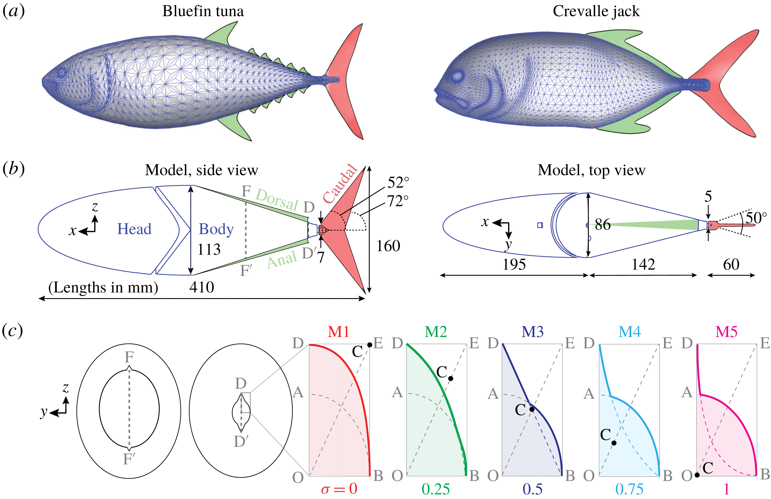
A reduced-order fish model was based on data from live tuna. (a) Bluefin tuna and crevalle jack reconstructions from Liu et al. (Reference Liu, Ren, Dong, Akanyeti, Liao and Lauder2017). (b) Reduced-order model used in this study (lengths in mm). The highlighted cross-sections (F-F
 $^{\prime }$
and D-D
 $^{\prime }$
) are shown in (c), and cross-section D-D
 $^{\prime }$
is used to define sharpness. (c) Sharpness (
 $\unicode[STIX]{x1D70E}\equiv 1-OC/OE$
) varied from 0 to 1 between the five models (M1–M5). Solid lines show the cross-sections of the body plus fin for each model, while dotted lines show the base ellipse (semi-axes OA and OB) and the Bezier curve (end points B and D, control point C) used to define the cross-section.
 $OA=0.97~\text{cm}$
,
 $OB=0.74~\text{cm}$
,
 $OD=1.73~\text{cm}$
.

In many high-speed carangiform and thunniform species, the dorsal and/or anal fins are elongated, stretching over a large portion of the fish’s proximal margin. In the crevalle jack (caranx hippos), for example, thin dorsal and anal fins stretch along nearly the entire back half of the fish (figure 1
a, Liu et al.
Reference Liu, Ren, Dong, Akanyeti, Liao and Lauder2017). In mackerel and tuna, an array of small dorsal/anal ‘finlets’ sits upstream of the caudal fin (Collette & Nauen Reference Collette and Nauen1983). For notational convenience, we will henceforth discuss ‘dorsal’ fins, but all results apply equally to elongated anal fins. Because of their close proximity to the caudal fin, these elongated dorsal features are likely to produce a strong interaction, because fin–fin interactions drop off quickly with distance (Boschitsch et al.
Reference Boschitsch, Dewey and Smits2014). Immersed-boundary-method-based flow simulations by Liu et al. (Reference Liu, Ren, Dong, Akanyeti, Liao and Lauder2017) suggest that in the crevalle jack, the elongated dorsal fin increases caudal fin thrust by 13.4 %. The simulations show that the caudal fin constructively interferes with vorticity shed from the dorsal fin. Zhu et al. (Reference Zhu, Wolfgang, Yue and Triantafyllou2002) used a three-dimensional potential flow solver to study dorsal–caudal interactions in a tuna-like model. They found that far-field wake modes depend on the phase lag between the dorsal and caudal fins, suggesting phase-dependent fin interactions. For these simulations, the Reynolds number based on swimming speed and whole body length is a limiting factor; whereas real fish may swim with
 $Re\sim O(10^{4}){-}O(10^{5})$
, in those studies
 $Re$
was 2100 (immersed-boundary-method) and effectively infinite (potential flow solver).
To explore the interaction between elongated dorsal fins and caudal fins, we tested a three-dimensionally (3-D) printed fish body in a water channel and compared results with immersed boundary simulations. The shape and kinematics of the model are based on bluefin tuna, and the dorsal fin is an idealized triangular shape. The resulting set-up allowed us to study the 3-D wake of an idealized dorsal fin on a realistic fish body at a realistic Reynolds number. What we found is that while wake capture plays a role, a more dominant feature is a dorsal-fin-induced cross-flow (DFC) that stabilizes the leading edge vortex against the caudal fin. This stabilized flow appears to prolong the thrust-producing section of the caudal fin’s flapping cycle, resulting in higher swimming speeds.
2 Experimental methods
2.1 Fish model design and construction
Using videos of live bluefin tuna, we reconstructed 3-D body kinematics using the same procedure as we have used previously (Bode-Oke, Zeyghami & Dong Reference Bode-Oke, Zeyghami and Dong2017; Liu et al.
Reference Liu, Ren, Dong, Akanyeti, Liao and Lauder2017). To facilitate comparisons with fish whose elongated dorsal features are simpler, such as the crevalle jack, we chose an archetypal elongated dorsal fin: a long triangular fin whose height is equal to that of the most distal finlet. The fin was mirrored on the bottom side of the fish to allow wake studies far from any influence of the sting supporting the model. We also eliminated other morphological details that could affect the flow on the caudal fin, such as the keel and the large dorsal fin upstream of the finlets. Our resulting reduced-order fish model is based on 11 key measurements of the high fidelity tuna model (figure 1
a,b) and has a whole body length
 $\ell$
of
 $410~\text{mm}$
. This reproducible model captures the major geometrical features of the original, including elongated dorsal features just upstream of the caudal fin.
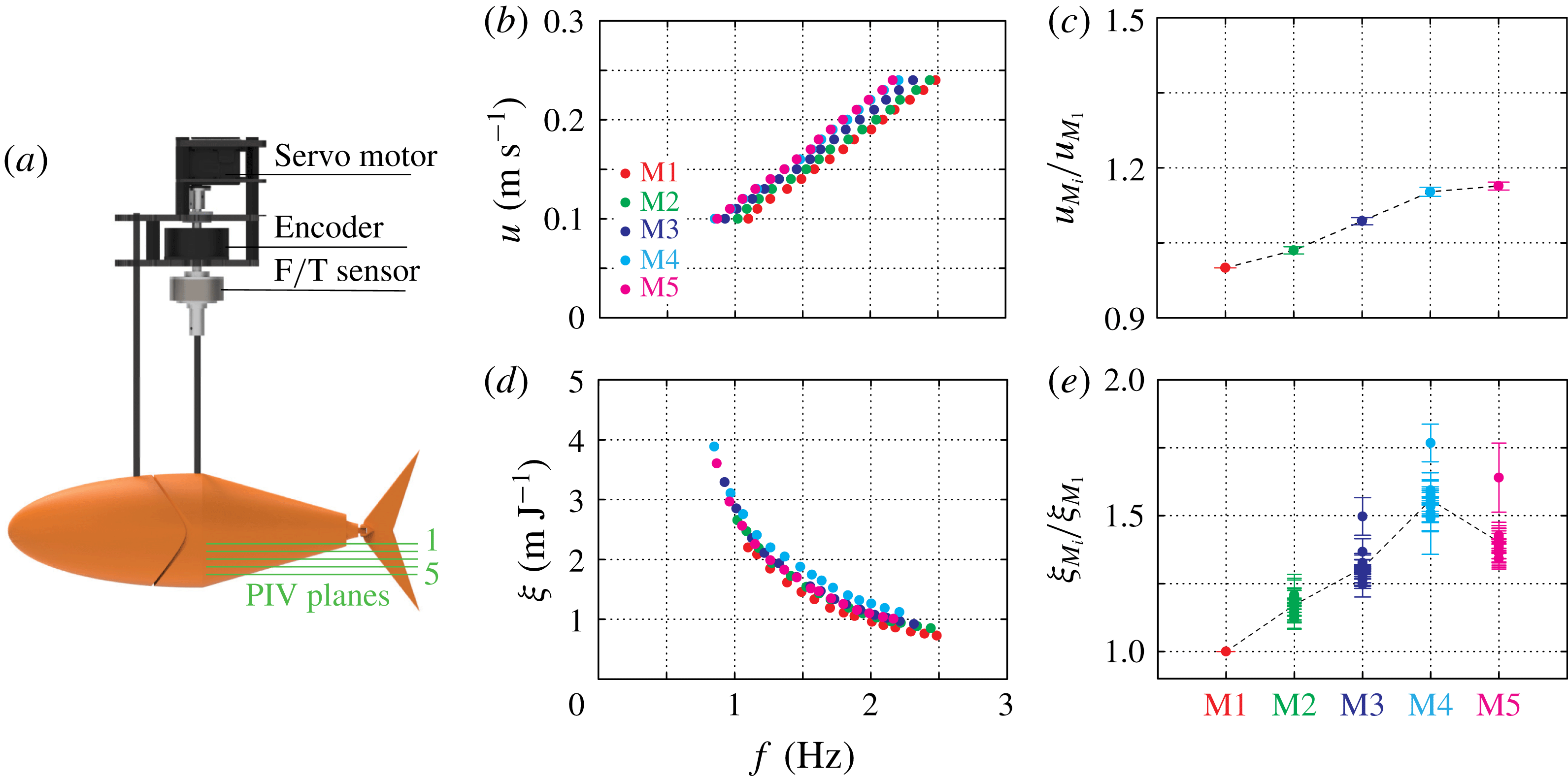
Swimming speed increases with sharpness, while economy peaks for M4. (a) A servo motor actuated the back half of the model (the ‘body’), and an encoder and F
 $/$
T sensor recorded angular displacement and
 $z$
-torques. Particle image velocimetry planes 1-5 are used to investigate flow features in figure 3. Self-propelled swimming speed increases linearly with frequency for each model. (c) Compared to M1, self-propelled speed increases from M1 to M4, but shows no noticeable difference between M4 and M5. (d) Propulsive economy,
 $\unicode[STIX]{x1D709}\equiv u/\overline{p}$
, decreases with frequency for each model. (e) Compared to M1, economy increases from M1 to M4, then decreases from M4 to M5. See appendix B for cycle-averaged power plots.

The tuna model was 3-D printed as two parts: a fixed head and an actuated body (figure 1
b). The head of the model was fixed in place by a 6.35 mm diameter carbon fibre rod, while the body was actuated by 6.35 mm diameter carbon fibre drive rod (figure 2
a). The drive rod, driven by a high torque digital servo motor (Dynamixel MX-64), twisted with harmonic pitching motions, that is,
 $\unicode[STIX]{x1D703}=\unicode[STIX]{x1D703}_{0}\sin (2\unicode[STIX]{x03C0}ft)$
, where
 $\unicode[STIX]{x1D703}$
is pitch angle,
 $\unicode[STIX]{x1D703}_{0}$
is pitch amplitude,
 $f$
is pitch frequency and
 $t$
is time. The caudal fin was actuated indirectly through a passive hinge joint (figure 1
b). Since fish are typically frequency rather than amplitude modulators (Nashimoto Reference Nashimoto1980; Rohr & Fish Reference Rohr and Fish2004), we set pitch amplitude to a constant
 $13^{\circ }$
based on the tuna videos (peak-to-peak fin excursion
 $a\approx 0.2\ell$
). The hinge joint of the caudal fin restricted peak-to-peak caudal fin angles to be less than
 $50^{\circ }$
(figure 1
b).
The ‘sharpness’ (
 $\unicode[STIX]{x1D70E}$
) of the dorsal fin was parameterized with Bezier curves, which allows continuous sharpness values ranging from 0 (no fin) to 1 (‘razor-thin’ panel) (figure 1
c). We considered five sharpness values for this study:
 $\unicode[STIX]{x1D70E}=0,0.25,0.50,0.75$
and
 $1$
. The cross-section of the model is the union of the area under the Bezier curves and a base ellipse, which forces the laterally projected areas of the models to be the same. A constant area means that differences in thrust between the models come from differences in fin geometry, not simply from changes in the total lateral width of the body and fin. The body and head of the tuna model were 3-D printed with acrylonitrile butadiene styrene (ABS) material (Dimension 1200es) which is effectively rigid over the frequencies and amplitudes considered here (see appendix A). To avoid different moments of inertia between the models (M1–M5), we kept the total mass of the model constant (
 $222.52\pm 3.46~\text{gm}$
). An absolute encoder (US Digital A2K 4096 CPR) verified that body motions were indeed the same between models for the same excitation (less than 0.2 % and 0.5 % variation in measured pitching amplitude and frequency).
2.2 Speed and economy measurements
To compare the swimming performance of the fin types, we measured the forces and torques on the tuna model while it was suspended in the
 $380\times 450\times 1520~\text{mm}\;(W\times H\times L)$
test section of a closed-loop water channel (Rolling Hills 1520). Tests were done at the centre of the channel, where the distance to sidewalls was
 ${\approx}2.4$
and
 ${\approx}6.3$
times the maximum span and maximum chord of the tail fin. These distances are high enough to avoid sidewall effects based on previous studies (Quinn et al.
Reference Quinn, Moored, Dewey and Smits2014; Fernández-Prats et al.
Reference Fernández-Prats, Raspa, Thiria, Huera-Huarte and Godoy-Diana2015). The head of the tuna model was mounted independently from the body, so the cycle-averaged streamwise force on the entire tuna model, or ‘net thrust’ (
 $\overline{T}$
), is the sum of the drag on the head (
 $D_{head}$
) and the cycle-averaged streamwise force on the body (
 $\overline{F}_{x}$
). We first measured
 $D_{head}$
as a function of channel speed by suspending the head from a high resolution one-axis force sensor (Interface Inc., ULC Ultra Low Capacity Load Cell, 1 N). We then measured
 $\overline{F}_{x}$
using a six-axis force sensor (ATI Mini-40, SI-80-4) installed along the drive rod. The measured forces were converted from sensor coordinates to test section coordinates and cycle-averaged over 30 pitching cycles to get
 $\overline{F}_{x}$
.
We chose to focus on steady swimming speeds, where the net thrust (
 $\overline{T}$
) is zero. Based on preliminary tests at tuna-inspired frequencies, we chose 15 steady swimming speeds (
 $u$
) evenly spaced between
 $100~\text{mm}~\text{s}^{-1}$
and
 $240~\text{mm}~\text{s}^{-1}$
(
 $0.24{-}0.59\ell ~\text{s}^{-1}$
), meaning the Reynolds number based on whole body length ranged from
 $Re=41\,000$
to 98 400. At each swimming speed, we used a Newton–Raphson-based zero-finding scheme to determine the pitching frequency
 $f$
that produced zero net thrust. Each iteration of the scheme consists of a warm-up period (5 pitching cycles), a data-acquisition period (30 pitching cycles), and a cooling period (1 s). After two initial guesses for
 $f$
, the scheme chooses the next frequency as the intercept of a
 $f(\overline{T})$
line fitted through the two guesses. This process iterates until net thrust is less than
 $2~\text{mN}$
, which was considered steady swimming within the uncertainty of the system. The scheme and subsequent measurements were applied to each swimming speed five times.
At each steady swimming speed, we measured the propulsive economy, which is a measure of the model’s range, or distance travelled per unit energy. Propulsive economy is defined as
 $\unicode[STIX]{x1D709}=u/\overline{p}$
, where
 $\overline{p}$
is the cycle-averaged hydrodynamic power transferred to the fluid. Cycle-averaged power is calculated by averaging
 $\unicode[STIX]{x1D70F}_{z}\dot{\unicode[STIX]{x1D703}}$
over 30 cycles, where
 $\unicode[STIX]{x1D70F}_{z}$
is
 $z$
-axis torque and
 $\dot{\unicode[STIX]{x1D703}}$
is pitching velocity as measured by the absolute encoder. To synchronize the
 $\unicode[STIX]{x1D703}$
and
 $\unicode[STIX]{x1D70F}_{z}$
signals, we recorded them directly to a custom circuit that transmitted the merged signals via wifi (ATI Wireless F/T) to a control PC (Omen 870).
2.3 Flow field measurements
To study the hydrodynamic interactions between dorsal and caudal fins, we used multi-layer stereo particle image velocimetry (PIV) to measure the flow fields around the tuna-inspired models. We measured multiple layers by keeping the laser sheet stationary and raising/lowering a custom automated
 $z$
-traverse (
 $2.5~\unicode[STIX]{x03BC}\text{m}$
resolution). We measured five layers, starting at the midline and decreasing in height by 7.5 mm per layer (figure 2
a). Because the fish model was symmetric about its midline, the bottom four layers were mirrored to estimate the wake on the upper half. The flow was seeded with neutrally buoyant polyamide seeding particles with an average diameter of
 $12~\unicode[STIX]{x03BC}\text{m}$
. Particles were illuminated by two overlapping laser sheets generated by 5 W and 10 W continuous lasers (MGL-W-532, Raypower and MGL-W-532A, CNI), firing from opposite sides to avoid a shadow. Two cameras beneath the channel (Phantom, SpeedSense M341) recorded
 $2956\times 1877~\text{px}$
images of the particle motions. The flow field analysis was performed by an adaptive PIV algorithm (Dantec Dynamic Studio 6.1) using interrogation windows ranging from
 $16\times 16~\text{px}$
to
 $64\times 64~\text{px}$
with
 $32\times 32~\text{px}$
grid step size. When reporting vorticity and velocity plots, we phase-averaged 75 pitching cycles over 3000 frames for each layer. Phase-averaging was done in Matlab (2018a), and three-dimensional vorticity/velocity plots were created in Tecplot (2017R2).
2.4 Immersed-boundary method simulations
To test which flow features were insensitive to Reynolds number, we compared our experiments to simulations from an in-house immersed-boundary method solver (see Liu et al. (Reference Liu, Ren, Dong, Akanyeti, Liao and Lauder2017), Zhong et al. (Reference Zhong, Liu, Ren and Dong2017), Zeyghami et al. (Reference Zeyghami, Zhong, Liu and Dong2018) for details). The simulations used identical geometries and kinematics as the experiments, the only difference being a lower Reynolds number based on whole body length
 $(Re=2100)$
. The solver used a non-uniform
 $385\times 193\times 193$
Cartesian grid (about 14 million points) over a computational domain of
 $10\ell \times 6\ell \times 6\ell$
. A cubic volume around the caudal fin used a high-resolution grid (
 $0.003125\ell \times 0.00278\ell \times 0.00375\ell$
spacing) to resolve the near-field wake structure. The mesh size was chosen based on extensive tests of mesh refinement combined with experience validating the solver on similar geometries (Liu et al.
Reference Liu, Ren, Dong, Akanyeti, Liao and Lauder2017).
3 Results
3.1 Sharpness affects swimming speed and economy
Up to a critical sharpness level, sharper dorsal fins lead to faster swimming speeds. For each fin type, the model’s steady swimming speed scales linearly with pitching frequency (figure 2
b), a trend to be expected based on the classic swimming scalings of Bainbridge (Reference Bainbridge1958). As dorsal fin sharpness increases, this linear curve is shifted up and left. A sharper dorsal fin therefore leads to a higher swimming speed at the same pitching frequency, or the same swimming speed at a lower frequency. To better visualize the effect of sharpness, we fitted lines to the speed versus frequency data for each fin type
 $(R^{2}=0.996\pm 0.001)$
, then compared the slopes. Because all the lines have zero intercept (zero frequency leads to zero swimming speed), the ratio of the slopes gives a measure of how much faster the model swims with a dorsal fin versus without a dorsal fin. Specifically, the ratio estimates
 $u_{Mi}/u_{M1}$
averaged over all frequencies, where
 $u_{Mi}$
is the swimming speed of the
 $i$
’th fin type and
 $u_{M1}$
is the swimming speed of the control case (
 $\unicode[STIX]{x1D70E}=0$
) at the same pitching frequency. As sharpness increases from 0 to 0.75, this ratio increases by about 15 %, but then saturates; increasing the sharpness further has no measurable result on swimming speed (figure 2
c).
While the swimming speed plateaus with increasing sharpness (figure 2
c), the economy peaks at a sharpness value between 0.5 and 1 (figure 2
e). The economy decreases monotonically with pitching frequency, again consistent with classic scalings (Bainbridge Reference Bainbridge1958) (figure 2
d). To better visualize the effect of sharpness, we calculated
 $\unicode[STIX]{x1D709}_{Mi}/\unicode[STIX]{x1D709}_{M1}$
, where
 $\unicode[STIX]{x1D709}_{Mi}$
is the economy of the
 $i$
th fin type and
 $\unicode[STIX]{x1D709}_{M1}$
is the economy of the control case (
 $\unicode[STIX]{x1D70E}=0$
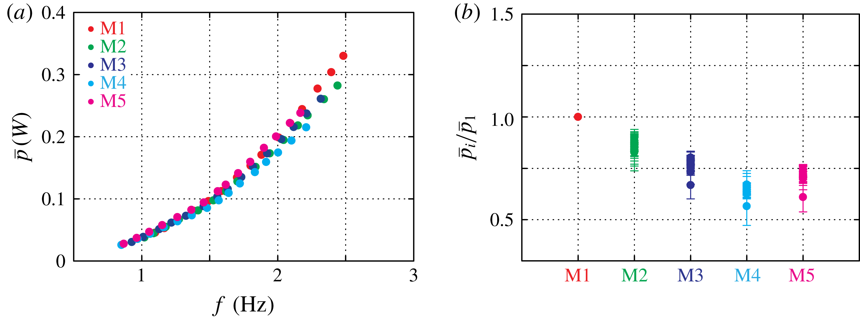
) at the same swimming speed. The ratio gives a measure of how much more efficiently the model swims with a dorsal fin versus without a dorsal fin at the same speed. As sharpness increases from 0 to 0.75, the economy increases significantly: it rises by about 50 % for most of the swimming speeds and up to 75 % at the slowest speed considered (figure 2
e). In contrast, economy decreases slightly as sharpness increases further, showing that economy peaks somewhere between
 $\unicode[STIX]{x1D70E}=0.5$
and
 $\unicode[STIX]{x1D70E}=1$
. Motivated by this peak in economy, we mapped the flow features governing the dorsal–caudal fin interaction and compared them across M1, M3, M4 and M5.
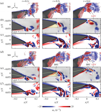
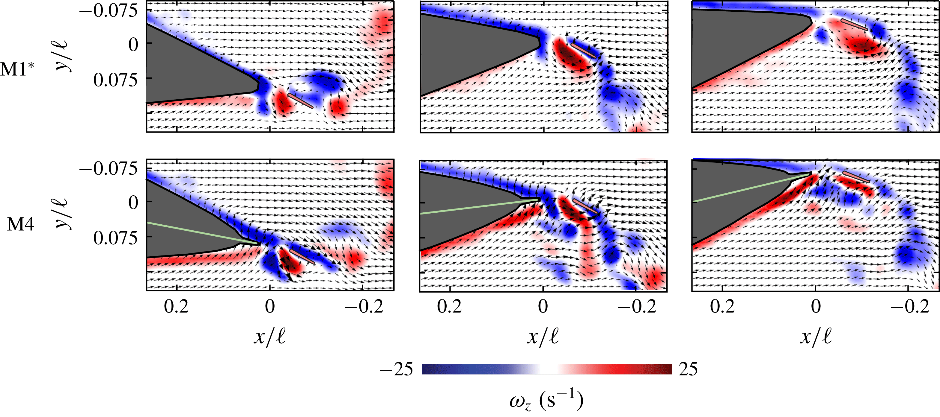
Both PIV and simulations reveal a more stable LEV on the caudal fin. Results are shown at self-propelled swimming for M1 (a–c) and M4 (d–f) at three times in the flapping cycle
 $\unicode[STIX]{x1D70F}$
:
 $t=0.1\unicode[STIX]{x1D70F}$
,
 $0.3\unicode[STIX]{x1D70F}$
, and
 $0.4\unicode[STIX]{x1D70F}$
). (a,d) Nine stacked layers of phase-averaged
 $z$
-vorticity show how the LEV separates from the caudal fin around
 $t=0.3\unicode[STIX]{x1D70F}$
. (b,e) The third vorticity contour from the top (Layer 3), shows the separation event in more detail. In the case of M4, the sharp dorsal fin induces a cross-flow (known as DFC) which stabilizes the LEV on the caudal fin. The dotted triangular and rectangular regions are used for averaging flow speeds in figure 4. (c,f) Simulated
 $z$
-vorticity contours are shown at the same time steps. The simulations show a more stable flow on the caudal fin in M4, but the effect is less pronounced than in the experiments. See appendix B for PIV around M1
 $^{\ast }$
. See Movie 1 in the supplementary material at https://doi.org/10.1017/jfm.2019.612 for PIV animations.

3.2 Leading edge vortex is stabilized on the caudal fin
We first used PIV to compare the flow fields of M1 (the control case,
 $\unicode[STIX]{x1D70E}=0$
) to M4 (
 $\unicode[STIX]{x1D70E}=0.75$
) at an intermediate swimming speed (
 $u=170~\text{mm}~\text{s}^{-1}$
). What we found is that the leading edge vortex (LEV) of the caudal fin is both stronger and more stable in the M4 case (figure 3
b versus 3
e). Attached LEVs can lead to high transient lift forces (Eldredge & Jones Reference Eldredge and Jones2019), which in this case presumably enhance thrust and increase the swimming speed (figure 2
d). Compared to M1, M4 exhibits a stronger, narrower jet of fluid produced by the translating gap between the dorsal and caudal fins (figure 3
b,e;
 $t=0.1\unicode[STIX]{x1D70F}$
). This jet forms the LEV, which contains positive
 $z$
-vorticity (as seen by, e.g. Borazjani & Sotiropoulos (Reference Borazjani and Sotiropoulos2010) and Liu et al. (Reference Liu, Ren, Dong, Akanyeti, Liao and Lauder2017)). In M1, the LEV fully detaches, leaving a region of slow-moving fluid adjacent to the caudal fin (figure 3
a,b;
 $t=0.4\unicode[STIX]{x1D70F}$
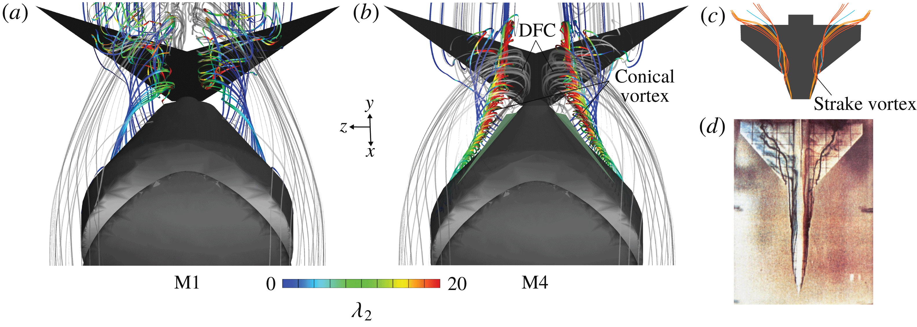
). In contrast, M4 exhibits a DFC that stabilizes the LEV along the caudal fin (figure 3
d,e;
 $t=0.4\unicode[STIX]{x1D70F}$
). The cross-flow energizes the boundary layer along the caudal fin, keeping the flow there attached longer in the pitching cycle.
By comparing the PIV results with immersed boundary method simulations, we found that major parts of these dorsal–caudal interactions persist at lower Reynolds numbers. The simulations, which simulate a lower
 $Re$
than the experiments (2100) but use the same geometry and Strouhal number (
 $fa/u$
), also show cross-flow induced by the sharp dorsal fin of M4 (figure 3
f). Like in the experiments, this cross-flow inhibits LEV detachment and energizes the boundary layer along the caudal fin. Unlike in the experiments, the negative
 $z$
-vorticity shed from the dorsal fin is confined to well-defined cores. In the experiments, these cores have mostly broken apart by
 $t=0.4\unicode[STIX]{x1D70F}$
(figure 3), as expected given the higher relative strength of inertial forces in the flow.
To quantify the DFC and the flow attachment on the caudal fin, we considered average flow speeds in two regions of the PIV data. Region 1 quantifies the strength of the cross-flow produced by the dorsal fin at
 $t=0.3\unicode[STIX]{x1D70F}$
, and region 2 quantifies how well the flow is attached to the caudal fin at
 $t=0.4\unicode[STIX]{x1D70F}$
(figure 3
b,e). In each region, we calculated
 $\overline{|\text{}\underline{v}|}/(fa)$
, where
 $\overline{|\text{}\underline{v}|}$
is the average in-plane flow speed in the region. This ratio, which represents how fast the flow is moving relative to typical lateral speeds of the fish model (
 $fa$
), allows a fair comparison of flow speeds between the models. Because the frequency is similar across models when
 $u=170~\text{mm}~\text{s}^{-1}$
(M1,
 $f=1.81~\text{Hz}$
; M3,
 $f=1.63~\text{Hz}$
; M4,
 $f=1.57~\text{Hz}$
; M5,
 $f=1.56~\text{Hz}$
), the denominator of the ratio does not vary more than
 $\pm 20\,\%$
across models. However, to ensure the scaling did not affect our conclusions, we also tested the M1 model at the flapping frequency of the M4 model and calculated
 $\overline{|\text{}\underline{v}|}/(fa)$
for both cases (notated as ‘M1’ and ‘M1*’).
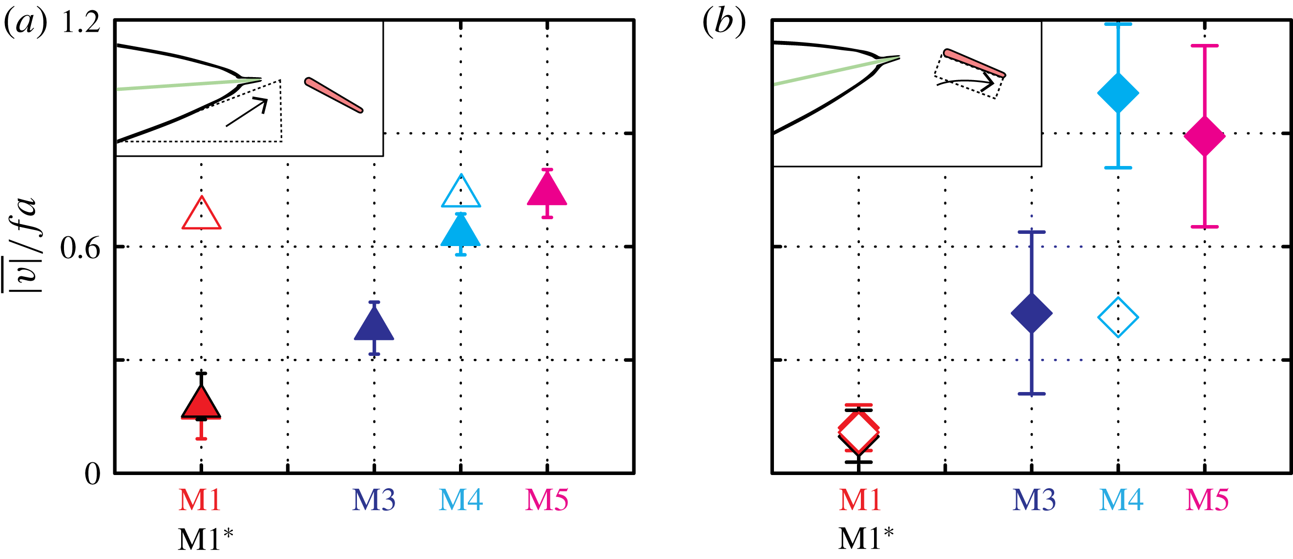
Average flow speeds in regions 1 and 2 reveal that the DFC increases with fin sharpness (M1 to M5), but that caudal fin flow attachment saturates beyond M4 (figure 4). In the case of M1,
 $\overline{|\text{}\underline{v}|}/(fa)$
is less than 0.3 in both regions 1 and 2, denoting slow cross-flow and mostly stagnant flow adjacent to the caudal fin (figure 4
a,b). In region 1,
 $\overline{|\text{}\underline{v}|}/(fa)$
increases monotonically with sharpness, showing that sharper dorsal fins induce more cross-flow. In region 2, however,
 $\overline{|\text{}\underline{v}|}/(fa)$
increases with sharpness up to
 $\unicode[STIX]{x1D70E}=0.75$
(M4), but shows no further increase beyond
 $\unicode[STIX]{x1D70E}=0.75$
. The similarities between the M1 and M1* cases show that these differences are due to dorsal fin geometry, not to the 13 % difference between the self-propelled pitching frequencies of M1 and M4. The low
 $Re$
simulations show similar trends but with a lower magnitude. Dorsal fin sharpness appears to increase swimming speed and economy by promoting flow attachment, but – beyond a critical sharpness – only costs more power without further improving the flow characteristics over the caudal fin. While the cross-flow is clearly visible in two-dimensional (2-D) PIV slices (figures 3
e, 4
a), the origins of the cross-flow can only be seen with a 3-D flow analysis.
Dorsal-fin-induced cross-flow increases with fin sharpness, while flow attachment on the caudal fin peaks at M4. (a) Dorsal-fin-induced cross-flow is quantified by the average flow speed (
 $\overline{|\text{}\underline{v}|}$
) in the triangular region in figure 3(b,e) (
 $t=0.3\unicode[STIX]{x1D70F}$
). To facilitate a fair comparison across models, speed was normalized by
 $fa$
. Filled symbols, PIV; empty symbols, simulations. (b) The stabilization of the flow on the caudal fin was quantified by the average flow speed in the rectangular region in figure 3(b,e) (
 $t=0.4\unicode[STIX]{x1D70F}$
). Flow attachment increases from M1 to M4 but shows no further increase from M4 to M5.

Long, thin, conical vortices are shed from sharp dorsal fins, causing a lateral cross-flow towards the caudal fin. Flows were visualized by mapping streamlines from the simulation results on M1 (a) and M4 (b) at
 $t=0.4\unicode[STIX]{x1D70F}$
. In M4, streamlines seeded on the dorsal side of the body (25 uniformly seeded on the dorsal fin), coloured by the
 $\unicode[STIX]{x1D706}_{2}$
criterion, are wound into tightly packed vortices that move downstream and over the caudal fin. Streamlines seeded upstream (50 seeded upstream of the head), coloured in light grey, show how these vortices induce a flow toward and along the caudal fin in M4 but not in M1. (c) Wing strake vortices (orange) shown passing over the main wing (schematic adapted from Reznick & Flores (Reference Reznick and Flores1989)). (d) Dye injection reveals strake vortices promoting flow attachment over an F-16A model in a water channel. Angle of attack,
 $15^{\circ }$
. Reynolds number, 15 000. Reprinted with permission from Reznick & Flores (Reference Reznick and Flores1989).

3.3 Sharp dorsal fins create streamwise conical vortices
To explore the origins of the DFC, we used the simulation results to map 3-D streamlines. Streamlines seeded on the dorsal fin reveal long, thin, conical vortices (figure 5
b). These vortices are visible as patches of negative vorticity in the stacked PIV slices for M4 (figure 3
d). The two vortices narrow, strengthen and move towards each other as they pass over the caudal fin. In contrast, the M1 case shows no such vortices (figure 5
a). Streamlines seeded upstream of the body reveal a key consequence of the tightly packed vortices: the surrounding water is moved laterally toward the caudal fin, then along the fin in a spanwise flow. This lateral flow towards the caudal fin is consistent with the 2-D PIV, where the cross-flow towards the caudal fin was observed in the
 $x$
–
 $y$
plane (figure 3
e).
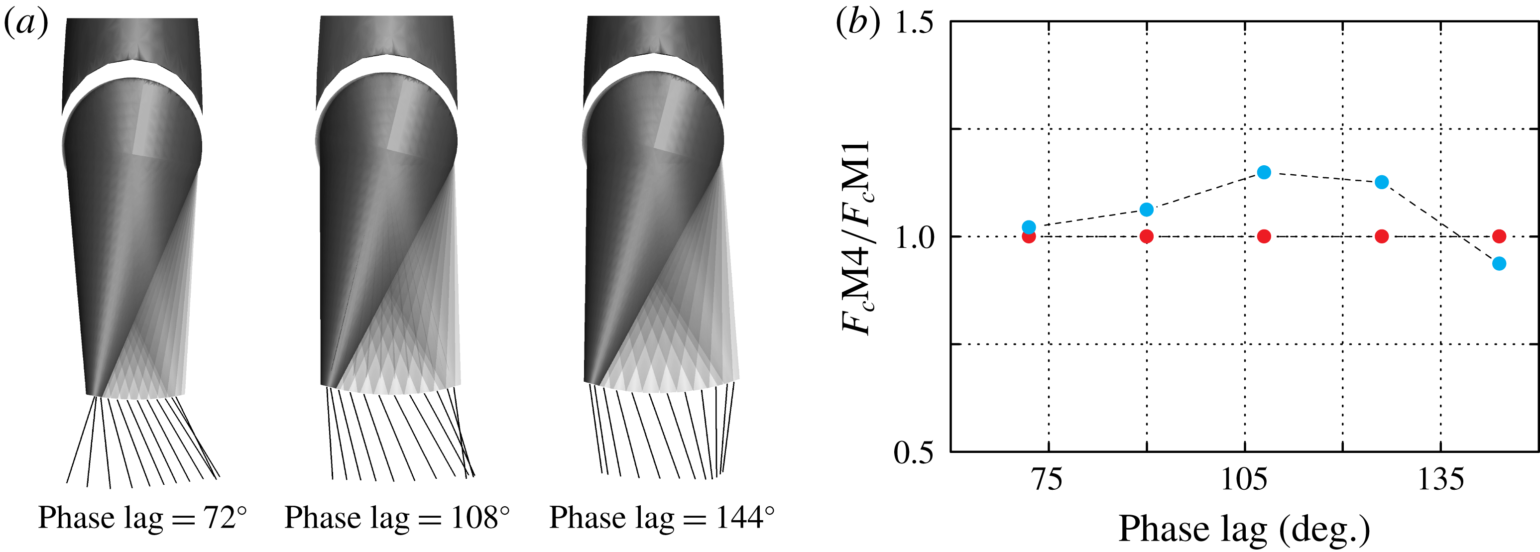
One consequence of the vortex-driven mechanism in figure 5 is that LEV-stabilization should be relatively insensitive to the phase lag between the dorsal and caudal fins. In the experiments, the phase lag follows from the passive mechanics of the caudal fin; in the simulations, phase lag is prescribed based on high-speed video of the experiments. Therefore, to explore phase sensitivity, we re-ran the simulations with manually adjusted caudal fin phase. We considered four perturbations from the original phase lag (
 $126^{\circ }$
):
 $72^{\circ }$
,
 $90^{\circ }$
,
 $108^{\circ }$
and
 $144^{\circ }$
. To make a fair thrust comparison, we matched the Strouhal numbers to the original by tuning pitching amplitude
 $\unicode[STIX]{x1D703}_{0}$
. The thrust increase between M1 and M4 was mostly positive over this range (
 $72^{\circ }$
,
 $+2.4\,\%$
;
 $90^{\circ }$
,
 $+6.3\,\%$
;
 $108^{\circ }$
,
 $+15\,\%$
;
 $126^{\circ }$
,
 $+13\,\%$
,
 $144^{\circ }$
,
 $-6.3\,\%$
; see appendix B). The mechanism is indeed robust to changes in phase up to around a quarter of the flapping cycle. Beyond that, the caudal fin’s lateral velocity presumably becomes out of sync with the stabilizing cross-flow provided by the dorsal fin.
4 Discussion
In our study, the LEV of the caudal fin starts stronger and stays attached longer in M4 compared to M1 (figures 3 e, 4 b, 7), and M4 swims faster than M1 (figure 2 e). These observations are consistent with previous findings that leading edge vortices can increase thrust when attached to the caudal fin (e.g. Borazjani & Daghooghi Reference Borazjani and Daghooghi2013). In heaving and pitching motions, leading edge vortices are shed soon after formation (Manar et al. Reference Manar, Mancini, Mayo and Jones2015; Mancini et al. Reference Mancini, Manar, Granlund, Ol and Jones2015), causing a transient burst of high thrust. The stability of the LEV increases with rounder fin planforms, lower actuation frequencies, spanwise flow and lower angles of attack (Eldredge & Jones Reference Eldredge and Jones2019). Spanwise flows, for example, prolong LEV attachment – and consequently transient forces – on caudal fins (Borazjani & Daghooghi Reference Borazjani and Daghooghi2013) and rotating wings (Lentink & Dickinson Reference Lentink and Dickinson2009; Garmann & Visbal Reference Garmann and Visbal2014; Jardin Reference Jardin2017). Cycle-averaged thrust on fins can therefore be enhanced by strengthening leading edge vortices, increasing leading edge vortex stability, or both.
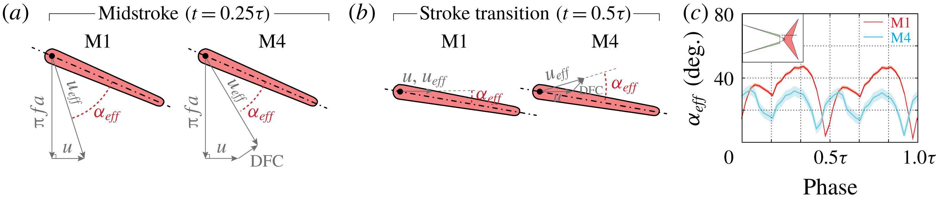
The DFC we observed affects the caudal fin’s angle of attack and creates spanwise flow along the caudal fin. Caudal fin shape is constant, and the pitching rates are similar (13 % difference between M1 and M4; 0 % between M1
 $^{\ast }$
and M4), so those two LEV stabilization mechanisms are less relevant here. The effective angle of attack, however, will often be lowered by the cross-flow, particularly at the centre of the caudal fin as it moves laterally (e.g.
 $t=0.3\unicode[STIX]{x1D70F}$
in figure 3
e). Through most of the pitching cycle, the effective angle of attack is lower for M4 than for M1 (e.g.
 $9^{\circ }\pm 6^{\circ }$
less at the mid-stroke,
 $t=0.5\unicode[STIX]{x1D70F}$
, appendix B). In contrast, at stroke transition (
 $t=0.5\unicode[STIX]{x1D70F}$
), the angle of attack is
 $16^{\circ }\pm 6^{\circ }$
higher for M4 than for M1. This higher angle may account for the stronger LEV created in M4 at the beginning of next stroke (
 $t=0.1\unicode[STIX]{x1D70F}$
, figure 3
e,b). We cannot measure spanwise flow quantitatively from the 2-D PIV slices, but
 $x$
–
 $y$
velocities along the caudal fin are nearly 10 times higher for M4 than for M1 (figure 4
b), and the simulated streamlines (figure 5
b) suggest spanwise velocities along the caudal fin are also higher. It appears that the cross-flow alters angle of attack and spanwise flow to create a stronger and more stable LEV for M4, which helps to explain its higher swimming speeds in the context of the known behaviour of leading edge vortices (Eldredge & Jones Reference Eldredge and Jones2019).
We suspect that a helpful analogue of the flow considered here is the flow over wing strakes and leading edge root extensions upstream of airplanes wings. Strakes are long thin surfaces that – like elongated dorsal fins – extend just upstream of the main lifting device (Shah Reference Shah1991). In aircraft design, ‘strake vortices’, which are shed from the elongated strakes, increase lift on the main wing during manoeuvres by lowering the angle of attack and promoting spanwise flow (figure 5
c,d). High lift devices on large aircraft function at higher Reynolds numbers (
 ${\sim}10^{6}$
based on wing chord, compared to
 ${\sim}10^{5}$
here), but given the qualitative similarities we observed across a decade of Reynolds numbers (figure 3), it may be that similar mechanisms are at work here. In fact, strake vortex flow visualizations are sometimes conducted at Reynolds numbers closer to
 $10^{4}$
(figure 5
c).
One key feature of the fin–fin interactions observed here is an insensitivity to the phase lag between dorsal and caudal fins. Our phase sensitivity tests reveal that the thrust boost in M4 persists over approximately a
 $70^{\circ }$
range of phase lags. Phase lag may be more relevant at lower Reynolds numbers, where vortices remain more coherent. Phase-dependent wake-capture mechanisms were reported, for example, in simulations of jack fish (Liu et al. (Reference Liu, Ren, Dong, Akanyeti, Liao and Lauder2017),
 $Re=2100$
). Phase lag may be especially important for isolated dorsal fins, like the main dorsal fin of the bluefin tuna (figure 1
a). For isolated upstream fins, the thrust of the downstream fin is only enhanced for certain combinations of fin placement and Strouhal number (Boschitsch et al. (Reference Boschitsch, Dewey and Smits2014),
 $Re=4700$
; Akhtar et al. (Reference Akhtar, Mittal, Lauder and Drucker2007),
 $Re=20\,000$
). At higher Reynolds numbers, disorganized, small-scale vortex structures reduce the possibility of constructive or destructive wake interactions (Daghooghi & Borazjani (Reference Daghooghi and Borazjani2015),
 $Re\approx 50\,000$
). Elongated dorsal fins – by inducing a phase-insensitive cross-flow – may boost thrust over a wider range of conditions.
A phase-insensitive mechanism also lends evidence to theories about the role of finlets. Finlets are thought to enhance the vortex circulation on caudal fins, thereby increasing thrust (Nauen & Lauder Reference Nauen and Lauder2002). They are also thought to serve as a fence that regulates cross-flow (Aleev Reference Aleev1969; Magnuson Reference Magnuson1970) and as a mechanism for redirecting flow and reducing separation along the caudal fin (Walters Reference Walters1962; Lindsey Reference Lindsey, Hoar and Randall1978). Our results show that the latter mechanisms (flow redirection) persist even for the simple case of one elongated ‘finlet’. The resulting caudal fin thrust enhancement may be further tuned by the complex morphologies and kinematics of finlets, some of which can be individually actuated (Nauen & Lauder Reference Nauen and Lauder2002).
5 Conclusion
Sharp, elongated dorsal/anal fins shed long, thin vortices that induce lateral cross-flow and stabilize the caudal fin’s LEV. This mechanism places dorsal–caudal fin interactions into a classical family of flows where cross-flows promote flow attachment on a lifting surface. At low Reynolds numbers, for example, laminar boundary layers are thinner, more stable, and less prone to detachment when there is wall suction (Iglisch Reference Iglisch1949; White & Corfield Reference White and Corfield2006). The flow in our case is unsteady, and the magnitude of cross-flow is much higher (
 ${\approx}0.5u$
compared to
 ${<}0.01u$
in Iglisch (Reference Iglisch1949)), but this general principle is empirically known to extend to high Reynolds numbers as well. For instance, active blown flaps and passive slats promote cross-flows that stabilize the flow over wings during fighter jet manoeuvres (Rudolph Reference Rudolph1996). Leading edge slats can be modelled as a simple vortex placed at the slat, inducing a cross-flow and promoting flow attachment on the main wing (Smith Reference Smith1975). We propose that elongated dorsal/anal fin geometries may be especially similar to strakes and leading edge root extensions, where thin fins on the fuselage create long, thin strake vortices that reduce angle of attack and promote spanwise flow (figure 5
c,d).
Dorsal–caudal fin interactions also offer new insights into the morphologies of fish and fish-inspired vehicles. By inhibiting flow separation on the caudal fin, the dorsal/anal fins increase swimming speed and economy, even if the laterally projected area is unchanged. The fins need not be razor-thin, because beyond a critical sharpness, the fins draw more power while having no noticeable effect on the flow along the caudal fin. Flow separation could also be inhibited by reducing tailbeat amplitude or frequency, but at the cost of reduced thrust. Not only does the mechanism observed here work at high thrust, it is relatively insensitive to phase lag. The Reynolds and Strouhal number ranges of our study (41 000–98 400 and 0.62–0.76) represent slow swimming compared to typical tuna cruise speeds, so the mechanism we observed may be most relevant at low speeds. However, given that the mechanism became more pronounced at higher Reynolds numbers, it may persist or even be stronger at higher speeds, where the fast-oscillating flow on the caudal fin is more prone to detachment. Either way, the mechanism provides a phase-insensitive, passive solution for improving the flow characteristics over oscillating propulsors, thereby offering design strategies for multi-fin, bio-inspired vehicles.
Acknowledgements
This work was supported by the Office of Naval Research under Program Director Dr. Robert Brizzolara, Award no. N00014-18-1-2537.
Supplementary material
Supplementary material is available at https://doi.org/10.1017/jfm.2019.612.
Appendix A. Dorsal fin stiffness scaling
Based on linear beam theory, dorsal fin deflection under a uniform load should be approximately
 $\unicode[STIX]{x1D6FE}h^{3}/(6EI)$
, where
 $\unicode[STIX]{x1D6FE}$
is force per length on the fin,
 $h$
is fin height,
 $E$
is fins elastic modulus (
 ${\approx}$
2 GPa for ABS) and
 $I$
is the area moment of inertia of the fin’s cross-section (
 $ld^{3}/12$
for a rectangular cross-section, where
 $l$
is fin length and
 $d$
is fin thickness). We can estimate the worst-case deflection using the highest lateral instantaneous force we recorded (3.1 N) and the thinnest dorsal fin (147 mm long, 7.6 mm high, and 1 mm thick). If the centre of pressure on the model were at the weakest part of the dorsal fin, we would expect the full 3.1 N to be applied over the 35 mm body span at that weakest point (2*OD in figure 1
c), resulting in a deflection of
 $$\begin{eqnarray}\frac{\unicode[STIX]{x1D6FE}h^{3}}{6EI}=\frac{\displaystyle 2\left(\frac{3.1~\text{N}}{35~\text{mm}}\right)(7.6\,\text{mm})^{3}}{(2~\text{GPa})(147~\text{mm})(1~\text{mm})^{3}}\approx 0.3~\text{mm}.\end{eqnarray}$$
Over the majority of trials, we expect much smaller deflections, because the lateral force goes with frequency squared, and the moment of inertia with fin thickness cubed. We also used a conservative estimate for
 $I$
by assuming a rectangular fin, whereas the actual dorsal fin is triangular. Therefore, we do not anticipate measurably different output kinematics for the same excitation, which we verified with high-speed camera images (figure 6).
Dorsal fin deflection is not measurably different between M1, M4 and M5. High-speed images taken at the same time (
 $t=0.25\unicode[STIX]{x1D70F}$
) and the same frequency (
 $f=1.57~\text{Hz}$
) show no observable differences in dorsal fin bending.

Appendix B. Supplemental figures
For self-propelled swimming, cycle-averaged power consumption decreases with sharpness until M4. (a) Cycle-averaged power consumption increases with frequency for each model. (b) Compared to M1, cycle-averaged power consumption decreases from M1 to M4, then slightly increases from M4 to M5.

Particle image velocimetry around M1
 $^{\ast }$
shows similar wake structures as PIV around M1 (figure 3
a,b).

Dorsal–caudal fin interaction is phase insensitive. (a) Top view of half-cycle time-lapsed kinematics of three phase lags considered (
 $72^{\circ }$
,
 $108^{\circ }$
,
 $144^{\circ }$
). (b) The ratio of M4 thrust to M1 thrust (
 $\overline{F}_{c}\text{M}4/\overline{F}_{c}\text{M}1$
) is mostly greater than 1 over the range of phase lags tested. Decreasing the phase from its natural value (126
 $^{\circ }$
) would require a stiffer tail joint; increasing the phase would require an actively controlled tail joint.

The effective angle of attack of the caudal fin is lower in M4 than in M1 for most of the pitching cycle. (a,b) Dorsal-fin-induced cross-flow decreases the effective angle of attack of the caudal fin at the midstroke and increases the effective angle of attack at stroke transition. (c) The effective angle of attack for M1 and M4 is shown through the full pitching cycle. Layer 3 (figure 3
b,e) was chosen to approximate the effective angle of attack of the caudal fin. The average speed of cross-flow was computed based on region 1 (figure 3
b,e) translated with the body. Angle uncertainty was estimated based on variability in the PIV vectors of region 1. The geometric angle of attack was calculated using high-speed video. Effective angle of attack was calculated as the angle of the effective incoming flow velocity (
 $u_{eff}$
), which was calculated using vector addition as follows. (a) M1 midstroke:
 $\unicode[STIX]{x1D6FC}_{eff}=\tan ^{-1}(\unicode[STIX]{x03C0}fa)/u-(25^{\circ }\pm 2^{\circ })=41^{\circ }\pm 2^{\circ }$
. M4 midstroke:
 $\unicode[STIX]{x1D6FC}_{eff}=\tan ^{-1}((\unicode[STIX]{x03C0}fa-(0.63\pm 0.08)fa\sin (55^{\circ }\pm 5^{\circ }))/(u+(0.63\pm 0.08)fa\cos (55^{\circ }\pm 5^{\circ })))-(25^{\circ }\pm 2^{\circ })=32^{\circ }\pm 4^{\circ }$
. (b) M1 at stroke transition:
 $\unicode[STIX]{x1D6FC}_{eff}=12^{\circ }\pm 2^{\circ }$
. M4 at stroke transition:
 $\unicode[STIX]{x1D6FC}_{eff}=\tan ^{-1}((0.6\pm 0.07)fa\sin (56^{\circ }\pm 4^{\circ })/(u+(0.6\pm 0.07)fa\cos (56^{\circ }\pm 4^{\circ })))+(12^{\circ }\pm 2^{\circ })=28^{\circ }\pm 4^{\circ }$
.