NOMENCLATURE
- c
specific heat capacity
- e
specific total energy
- h
specific enthalpy
- k.
turbulence kinetic energy
- l
length scale
- Mw
molar mass
- M
Mach number
- p
static pressure
- q
heat flux
- Pr
Prandtl number
- ℜ
universal gas constant
- T
static temperature
- u
mean velocity component
- v
mean velocity magnitude
- x
direction component
- y
normal distance to cell center
- γ
specific heat capacity ratio
- δij
Kronecker delta
- ε
dissipation rate of k
- κ
von Karman constant
- λ
thermal conductivity
- μ
viscosity
- ρ
density
- τ
viscous heating
Subscripts
- eff
effective
- j
Cartesian component
- k
turbulence kinetic energy
- op
operating condition
- p
constant pressure
- P
first node near wall
- t
turbulent
- v
constant volume
- w
wall
- ε
related to ε
- μ
related to μ
1.0 INTRODUCTION
A comprehensive thermal analysis of regeneratively cooled liquid rocket engine thrust chambers has been strongly benefited by the popularisation of CFD techniques, assuring the theoretical integrity of such components(Reference Marchi, Laroca, Silva and Hinckel1,Reference Naraghi, Dunn and Coats2) . The heat transfer in this type of thrust chambers under operating conditions involves: (a) heat transfer from the hot gas to inner wall, (b) heat conduction through chamber wall, and (c) convective heat transfer from chamber wall to coolant. To accurately predict the temperature in the cooling channel, particularly on the gas-side wall, all three domains must be simultaneously computed(Reference Knab, Frey, Görgen, Maeding, Quering and Wiedmann3,Reference Kirchberger, Hupferand, Kau, Soller, Martin, Bouchez and Dufour4) . In this sense, adequate understanding and accurate prediction of the conjugate heat transfer between hot gas, chamber wall, and coolant liquid is a prerequisite for thrust chamber designs(Reference Negishi, Kumakawa, Yamanishi and Kurosu5).
Common approaches found in the literature used to solve the conjugate conduction-convection problem separate it into two problems connected by one interface between the fluid and solid zones. The solution process usually starts by supposing a wall temperature distribution in the interface as a boundary condition for one zone and using the obtaining wall heat flux distribution as boundary condition for the other zone. Next, the resulting temperature distribution in the interface replaces the supposed temperature distribution used in the first step. The process repeats iteratively until the convergence of temperature and heat flux distributions in the interface. Experience has shown the efficiency of such an approach depends on how far the wall temperature distribution provided in the first step is from the solution. If the supposed values are quite far, the convergence can be slow or even cannot be found.
The main objective of the present study is to propose a unified approach to overcome the mentioned deficiencies, solving the conjugate convection-conduction problem with just one domain, comprising all fluids and solid zones, in order to find a preliminary solution addressed for deeper investigation. This approach has several advantages, since the iterative process between two domains is unnecessary, saving computational time and avoiding cumulative errors due to the use of a convection coefficient or heat flux calculation in each iteration.
Thus, computations are compared to test results obtained in a high-enthalpy wind tunnel facility at Arnold Engineering Development Center (AEDC) at Arnold Air Force Base, Tennessee, USA, for several gas and coolant flow conditions, as well as to results obtained by other authors who used the same set of experimental data and geometry as described below.
Shope(Reference Shope6) developed and extensively modified a space-marching boundary layer program to model conjugate conduction-convection heat transfer for the case of co-flowing high-speed gas and liquid coolant. Solid body conduction was modeled as one-dimensional, constant property heat transfer. The coolant was empirically modeled as a bulk fluid with combined forced convection and sub-cooled nucleate boiling. The flow solver was modified to solve the group of conjugate boundary equations simultaneously and implicitly with the existing momentum and energy equations for the gas. The theoretical water coolant temperature rise was shown to agree quite well with the measured temperature rise and nucleate boiling is predicted to be a crucial effect of the coolant.
Engblom et al(Reference Engblom, Fletcher and Georgiadis7) presented a structured-mesh heat transfer module named FOGO, coupled with two different compressible Reynolds-Averaged Navier-Stokes flow solvers named TBD and Wind-US, and predictions are compared against experimental data for various turbulence models and coolant modeling assumptions. FOGO is a finite-volume, cell-centered, multi-block, structured-mesh, 3D heat conduction solver, with submodels for solid body conduction, forced convection, and nucleate and film boiling. These submodels were configured for analysis of water-cooled high-speed flows. The temperature gradient of the solid was evaluated at each cell face using second-order spatial treatment. Coolant flow was treated as a separate three-dimensional zone which exchanges heat with a solid body zone. The nucleate boiling heat is a relevant mechanism when coolant temperatures reach liquid saturation conditions. The TBD solver can model thermally perfect, chemically reacting flows using conservative state vector with transport equations for each species, density, three momentum components, and total energy, plus additional equations for transport of turbulent kinetic energy and dissipation rate of turbulent kinetic energy. The Wind-US solver is a 3D chemically reacting, Reynolds-averaged Navier-Stokes (RANS), density-based compressible flow solver for inviscid fluxes computed using a true second-order Roe scheme, which accounts for grid stretching, and the solution uses local time stepping and a spatially split line-based factorisation scheme, with several turbulence models available. A combination of such solvers and the boiling process selection provided four different models: TBD/FOGO with nucleate boiling (model 1); TBD/FOGO with nucleate/film boiling (model 2); Wind-US/FOGO with nucleate boiling (model 3); and Wind-US/FOGO with nucleate/film boiling (model 4). Simulation results were compared using deviations from the experimental data.
Engblom et al(Reference Engblom, Fletcher and Georgiadis8) extended their studies, combining the mentioned 3D solvers Wind-US/FOGO with a new 2D, two-phase, axisymmetric, cell-centered, structured-grid, RANS pressure-based, SIMPLE scheme solver named COOL. The coupled Wind-US/FOGO/COOL package is successfully validated against existing data. The air is modeled as non-vitiated, 5-species reacting air (O2, NO, O, N, N2) using the chemical kinetics provide which account for molecular recombination, expected as the flow within the nozzle expands. The initial conditions are assumed to be in chemical equilibrium at the specified total temperature and pressure, and the species concentrations are predicted using software provided by Colorado State University. The water inlet pressure was 68 atm for each run. Thereby, the thermodynamic table used by COOL to look up fluid properties vs enthalpy is taken from NIST data along a 68 atm isobar. NIST assumes thermodynamic equilibrium at the coolant pressure and consequently has a discontinuity of enthalpy vs temperature during the liquid-vapor phase change. But the transition from liquid to vapor water flow involves complex fluid behaviour that is clearly not in thermodynamic equilibrium. Thus, the enthalpy is ‘smoothed’ over a 100K temperature interval starting at saturation condition.
Kang and Sun(Reference Kang and Sun9) used ANSYS Fluent to simulate the hot gas convective heat transfer separately from the conjugate heat transfer in the coolant and cooling channel in order to prevent numerical instability. A common inner wall temperature was used to assure the balance of heat flux at gas-solid interface, coupling both domains. A standard wall function was used to bridge the viscosity-affected region between the wall and the fully turbulent region. The RMS turbulence model was used to model the turbulent air and water flow. Two models were used to compare with experimental data: frozen flow, which considers the species concentration as constant through the nozzle (model 1); and non-equilibrium flow, which uses a finite rate chemistry to model the reactive flow through the nozzle (model 2). The gas is modeled as non-vitiated, non-equilibrium, five-species reacting air (O2, NO, O, N, N2). The initial conditions are considered to be in chemical equilibrium, and the species concentrations are predicted using a chemical equilibrium calculation program. Simulation results showed less heat flux in the case of frozen flow.
2.0 PROBLEM DESCRIPTION
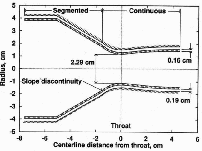
Experiments were performed in the wind tunnel at AEDC, a 40 MW segmented, electric arc-heated, high-enthalpy ablation test facility called HEAT-H1(Reference Shope6). In such a facility, air is continuously heated by passing an electric arc through a column of high-pressure air about 5 cm in diameter and about 2 m long. The heated air is expanded through a double wall, water-cooled, contoured, axisymmetric, supersonic nozzle, designed to provide a region of uniform flow. The test facility operates routinely at bulk stagnation conditions of 100 atm and 4,500°K, corresponding to 2.4 kg/s of air at about 7 MJ/kg. The nozzle geometry is modeled in a somewhat idealised form shown in Fig. 1.
Idealized nozzle geometry (Shope(Reference Shope6)).

The inner wall is made of a copper-zirconium (Cu-Zr) alloy with a 0.16 cm thickness and geometry consisting of a 7.6 cm inlet diameter, a 2.29 cm throat diameter and a 2.6 cm outlet diameter. Between the inner and outer walls, water flows confined into a narrow channel of 0.19 cm height.
The nozzle comprises two segments, with a small slope discontinuity about 1.6 cm upstream from the throat. The first nozzle piece, indicated as segmented, is composed of rings, with annular depressions in their interfaces. The second segment, indicated as continuous, is composed of an integral, smooth, contoured nozzle with an overall length of 5.8 cm, designed to provide parallel exit velocity with a Mach number of about 1.8. The roughness effects of the first segment on the second should be diminished by the acceleration of the gas in the contraction region, so the surface roughness is neglected.
Each nozzle segment has its own cooling water inlet and outlet and, for the present study, a continuous annular passage for coolant is assumed for each segment. The first segment inlet is placed at the beginning of the device and its outlet is placed at the position 1.6 cm upstream from the throat. Near the same point, the second segment inlet with an outlet located at the end of the nozzle is placed. Water inlet and outlet manifolds for the first and second segments are not shown in the picture.
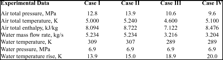
The experiments consist of four different entry conditions, depending on the total pressure and total temperature at the air inlet, as well as mass flow rate and static temperature at the water inlet in the second segment, as shown in Table 1.
Air and water flow conditions (adapted from Shope(Reference Shope6))
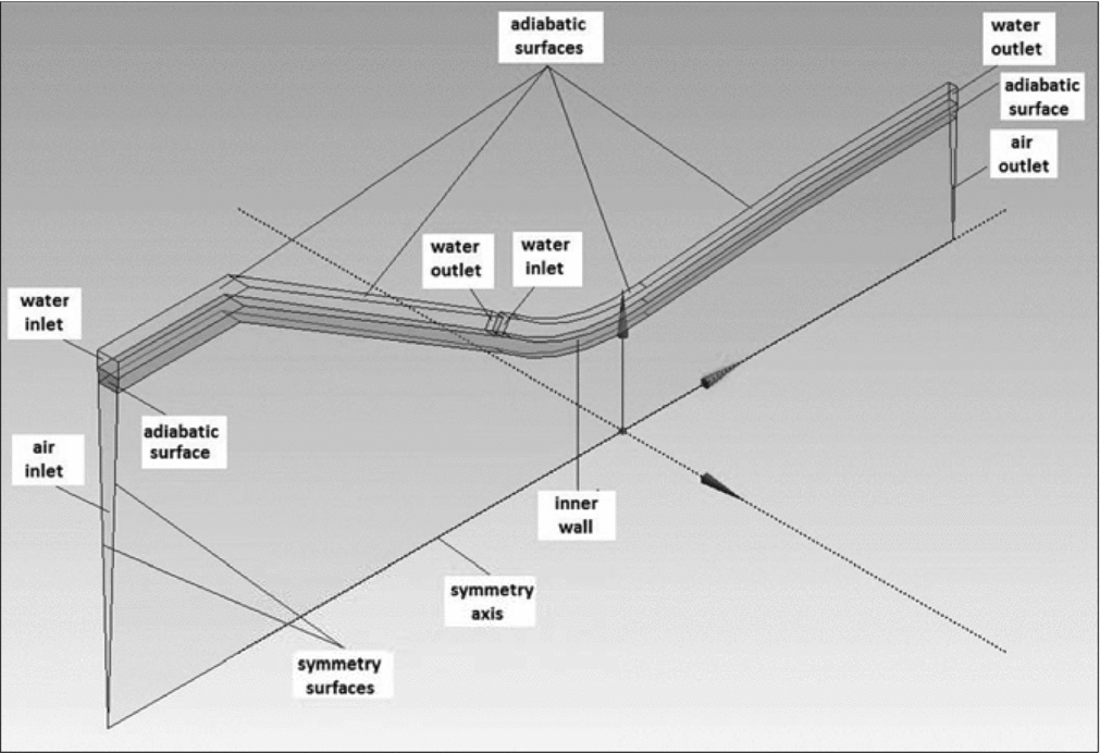
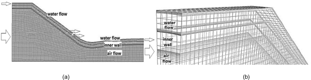
Figure 2 shows a 3.75° azimuthal slice along the nozzle modeled as multi-bodies, combining gas, inner wall and liquid regions in just one 3D domain. The outer wall has not been represented, since the surface in contact with water was stated as adiabatic. Water mass flow rate was simulated as 1/96 of the total mass flow rate to be compatible with the azimuthal slice of the nozzle.
Nozzle geometry used in the simulations.
3.0 MATHEMATICAL MODEL
The model consists of a compressible ideal gas and incompressible liquid flows, both in steady state, subjected to a conjugate convection-conduction heat transfer process. The following governing equations used in the simulations can be found in ANSYS Fluent Theory Guide(10):
3.1 Continuity equation
 $$\begin{equation}
\frac{\partial }{{\partial {x_j}}}\left( {\rho {u_j}} \right) = 0
\end{equation}$$
3.2 Momentum equation (RANS)
 $$\begin{equation}
\frac{\partial }{{\partial {x_j}}}\left( {\rho {u_i}{u_j}} \right) = - \frac{{\partial p}}{{\partial {x_i}}} + \frac{\partial }{{\partial {x_j}}}\left[ {{{\left( {{\tau _{ij}}} \right)}_{\text{eff}}} - \frac{2}{3}\rho k{\delta _{ij}}} \right]
\end{equation}$$
where  ${( {{\tau _{ij}}} )_{\text{eff}}} = {\mu _{\text{eff}}}( {\frac{{\partial {u_j}}}{{\partial {x_i}}} + \frac{{\partial {u_i}}}{{\partial {x_j}}} - \frac{2}{3}\frac{{\partial {u_k}}}{{\partial {x_k}}}{\delta _{ij}}} );\ {\mu _{\text{eff}}} = \mu + {\mu _t}$.
3.3 Energy equation
 $$\begin{equation}
\frac{\partial }{{\partial {x_j}}}\left[ {\rho \left( {e + \frac{p}{\rho }} \right){u_j}} \right] = \frac{\partial }{{\partial {x_j}}}\left[ {{\lambda _{\text{eff}}}\frac{{\partial T}}{{\partial {x_j}}} + {u_i}{{\left( {{\tau _{ij}}} \right)}_{\text{eff}}}} \right]
\end{equation}$$
where  $e = {c_p}T - \frac{p}{\rho } + \frac{{{v^2}}}{2};\ \quad {\lambda _{\text{eff}}} = \lambda + {\lambda _t};\ \ {\lambda _t} = \frac{{{c_p}{\mu _t}}}{{P{r_t}}};\quad P{r_t} = 0.85$.
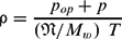
3.4 State equation (perfect gas)
 $$\begin{equation}
\rho = \frac{{{p_{op}} + p}}{{\left( {\mathfrak{N}/{M_w}} \right)\ T}}
\end{equation}$$
where pop = 0.1 MPa for compressible flow.
3.5 Turbulence model
It is assumed the k-ε model with modified ε-equation and variable turbulence viscosity (μt), named ‘Realisable k-ε Model’. As mentioned in the ANSYS Fluent Theory Manual(10), the transport equations for k and ε were originally developed by Shih et al(Reference Shih, Liou, Shabbir, Yang and Zhu11), in 1995:
 $$\begin{equation}
\frac{\partial }{{\partial {x_i}}}\left( {\rho k{u_i}} \right) = \frac{\partial }{{\partial {x_j}}}\left[ {\left( {\mu + \frac{{{\mu _t}}}{{P{r_k}}}} \right)\frac{{\partial k}}{{\partial {x_j}}}} \right] + \rho \varepsilon + {\mu _t}{S^2} - 2\rho \varepsilon M_t^2
\end{equation}$$\\
 $$\begin{equation}
\frac{\partial }{{\partial {x_i}}}\left( {\rho \varepsilon {u_i}} \right) = \frac{\partial }{{\partial {x_j}}}\left[ {\left( {\mu + \frac{{{\mu _t}}}{{P{r_\varepsilon }}}} \right)\frac{{\partial \varepsilon }}{{\partial {x_j}}}} \right] + \rho {C_1}S\varepsilon - \rho {C_2}\frac{{{\varepsilon ^2}}}{{k + \sqrt {\mu \varepsilon /\rho } }}
\end{equation}$$\\
 $$\begin{equation}
{\mu _t} = \rho {C_\mu }\frac{{{k^2}}}{\varepsilon }
\end{equation}$$
 $$\begin{equation*}
S = \sqrt {2{S_{ij}}{S_{ij}}} ;\;{S_{ij}} = \frac{1}{2}\left( {\frac{{\delta {u_j}}}{{\delta {x_i}}} + \frac{{\delta {u_i}}}{{\delta {x_j}}}} \right);\;{M_t} = \sqrt {\frac{k}{{\gamma RT}}}
\end{equation*}$$
 $$\begin{equation*}
{C_1} = {\rm{max}}\left[ {0.43,\frac{\eta }{{\eta + 5}}} \right];\ \eta = S\frac{k}{\varepsilon };S = \sqrt {2{S_{ij}}{S_{ij}}} ;\ {S_{ij}} = \frac{1}{2}\left( {\frac{{\delta {u_j}}}{{\delta {x_i}}} + \frac{{\delta {u_i}}}{{\delta {x_j}}}} \right)
\end{equation*}$$
 $$\begin{equation*}
{C_\mu } = \frac{1}{{{A_0} + {A_s}\frac{{k{U^*}}}{\varepsilon }}};\;{A_0} = 4,04;{U^*} = \sqrt {{S_{ij}}{S_{ij}}} ;\ {A_s} = \sqrt 6 {\rm{cos}}\phi
\end{equation*}$$
 $$\begin{equation*}
\phi = \frac{1}{3}{\rm{co}}{{\rm{s}}^{ - 1}}\left( {\sqrt 6 W} \right);W = \frac{{{S_{ij}}{S_{jk}}{S_{ki}}}}{{{{\bar S}^3}}};\ \bar S = \sqrt {{S_{ij}}{S_{ij}}}
\end{equation*}$$
3.6 Near-wall model
Enhanced Wall Treatment is a near-wall modeling method that combines a two-layer model with so-called enhanced wall functions. When the near-wall mesh is fine enough to be able to resolve the viscous sublayer, typically with the first near-wall node placed at y+ ≈ 1,then the traditional two-layer zonal model could be employed. However, the restriction that the near-wall mesh must be sufficiently fine everywhere instead of only at y+ ≈ 1 might impose too large a computational requirement. Ideally, one would like to have a near-wall formulation that could be used with coarse meshes (wall-function meshes) as well as fine meshes (low-Reynolds-number meshes).
In addition, excessive error should not be incurred for the intermediate meshes where y+ is placed neither in the fully turbulent region where the wall functions are suitable, nor in the direct vicinity of the wall at y+ ≈ 1, where the low-Reynolds-number approach is adequate. To achieve the goal of having a near-wall modeling approach that will possess the accuracy of the standard two-layer approach for fine near-wall meshes and that at the same time will not significantly reduce accuracy for coarse near-wall meshes, the Enhanced Wall Treatment model is herein used.
4.0 COMPUTATIONAL METHODOLOGY
The mathematical model equations were solved using ANSYS Fluent, Release 13.0, which is a CFD program based on finite volume method(10). A pressure-based scheme and SIMPLE pressure-velocity coupling method were selected. To assure the compromise between the solution stability and computational efforts, under-relaxation factors were set as follows: 0.3 for pressure, 0.7 for momentum, 0.8 for the turbulence kinetic energy and turbulence dissipation rate, and 1.0 for density, body forces, energy, and turbulent viscosity. In order to decrease false diffusion effects, spatial discretisation was set as follows: least squares cell based for gradient; second order for pressure; and second order upwind for density, momentum, energy, turbulent kinetic energy, and turbulent dissipation rate. Turbulence parameters were set considering an inlet turbulent intensity of 5% and a turbulent-to-laminar viscosity ratio equal to 10.
4.1 Boundary conditions
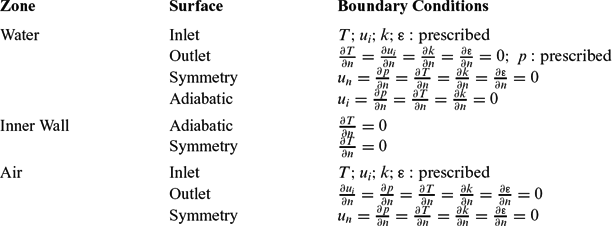
Boundary conditions have been specified for each external surface involving the domain, as shown in Table 2.
Specified boundary conditions
4.2 Initialisation values
All interior zones have been initialised with uniform null values. However, the inlet pressure of the airflow was initialised using a low value (0.01 MPa) and successively incremented up to the required experimental value (9.6 ~ 13.9 MPa). Hence, each new simulation used the previous solution as initialisation values.
4.3 Convergence criteria
Two criteria were used to determine the convergence:
a) stabilisation of average static pressure and temperature of the liquid and gas at the throat and outlet sections;
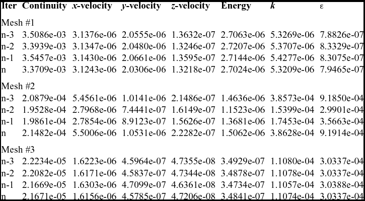
b) achievement of minimum third order relative residuals of continuity, x-velocity, y-velocity, z-velocity, energy, k and ε equations (Table 5).
5.0 MATERIAL PROPERTIES
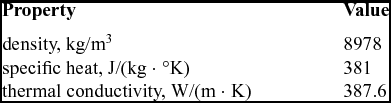
Table 3 shows the properties for the nozzle wall, considering a Cu-Zr alloy called USN.C15000. Properties at room temperature were used, since they are practically constant in a large range of operational temperatures.
Properties of Cu-Zr alloy
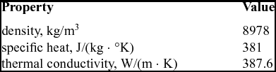
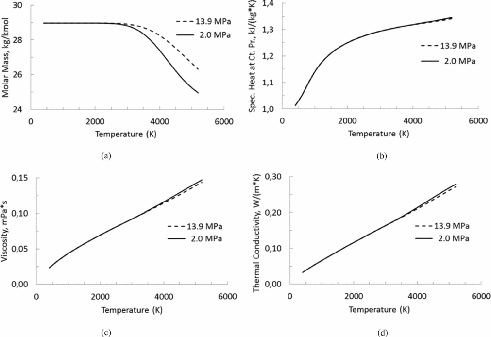
Figure 3 presents the behaviour of dissociated air in thermodynamic equilibrium depending on the temperature and pressure, where dissociated air consists of a mixture of main species: N2, O2, N2O, NO2, NO, O, N, and Ar. Property values of air were obtained from the National Aeronautics and Space Administration (NASA) online program CEARUN(Reference Gordon and Mcbride12). The perfect-gas approach considers that the fluid properties are only temperature-dependent. In accordance with the theory, it is possible to verify that the behaviour of the dissociated air is more sensitive to the temperature than to the pressure, as observed in the range of 2.0 MPa to 13.9 MPa that characterises the present simulations. Note the properties are not so influenced by the pressure, as expected for a perfect gas; then the properties are used in the simulations as functions depending just on the temperature, considering an average value between both pressure levels.
Properties of air: (a) molar mass, (b) specific heat at constant pressure, (c) viscosity, and (d) thermal conductivity.
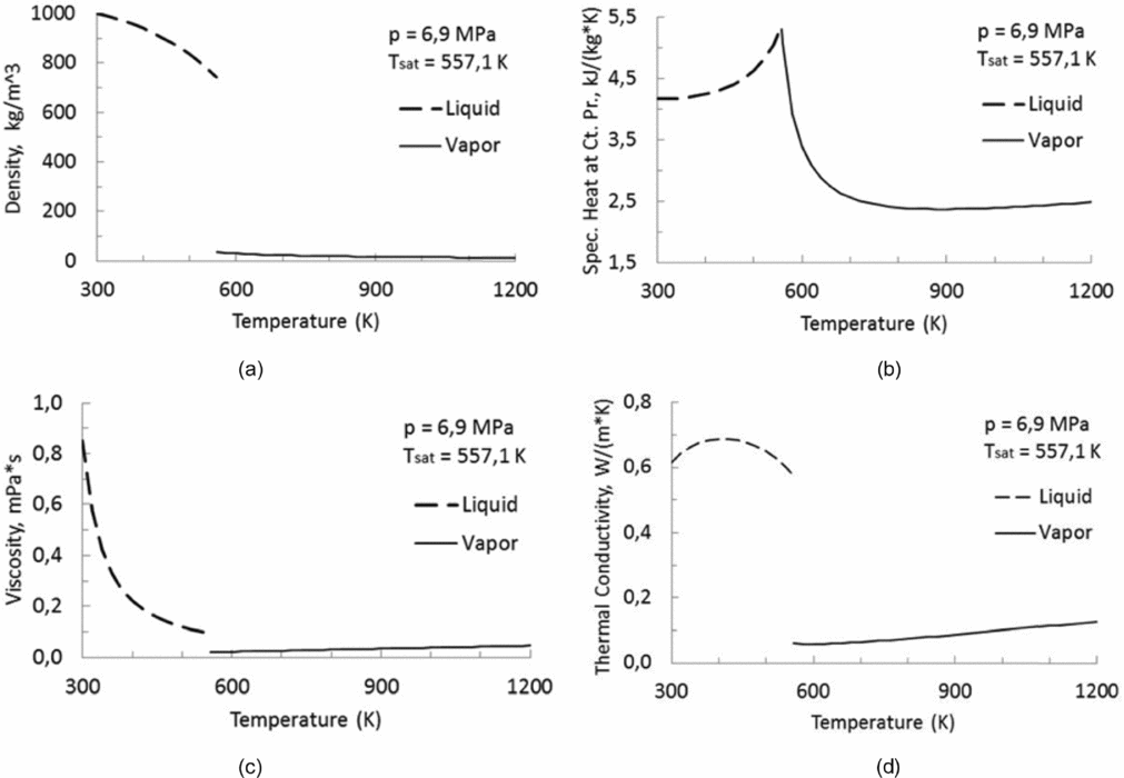
On the other hand, Fig. 4 presents the properties of compressed liquid and superheated vapor depending on the temperature for only one pressure level. Water property values were obtained from the National Institute of Standards and Technology (NIST) online program Chemistry Web Book(Reference Lemmon, Mclinden and Friend13). Although the pressure inside the cooling channels varies a little along the nozzle, the properties are practically invariant with respect to the pressure change, even in the presence of the vapor phase, so the properties used in the present simulations are also just temperature-dependent. It should be noted that the NIST tables assume thermodynamic equilibrium at a given pressure and, consequently, have a discontinuity of properties during the liquid-vapor phase change at the saturated temperature for that pressure.
Properties of water: (a) density, (b) specific heat at constant pressure, (c) viscosity, and (d) thermal conductivity.
Engblom et al(Reference Engblom, Fletcher and Georgiadis8) reported serious numerical instabilities when computing the sensible heat flux due to the discontinuity in enthalpy as a function of temperature. They solved the problem using a third order polynomial to fit this property, starting at the saturation condition, preserving the original values and slopes at end point set as the saturation temperature plus 100°K. The same kind of problem was found in this study when facing liquid- to vapor-phase change and the procedure used above was implemented in order to fit water properties with good results. Then, in the present study, the liquid-to-vapor phase change has been considered according to the water properties in each phase depending only on the temperature.
6.0 MESH VERIFICATION
Generated meshes employed the ANSYS Meshing package Release 13.0 using cut-cell meshing method, which is suitable for creating cells with low deformity(14). The meshes were clustered near the gas-side and liquid-side inner wall, as well as near the outer wall modeled as an adiabatic surface, using a geometric progression which increased each increment by a factor of 1.1 over the previous one totaling 10-cell layers. Figure 5 shows a lateral view and mesh refinement near the gas-side and liquid-side walls.
Mesh details: (a) lateral view (b) refinement near the wall.
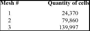
As usual in computational simulations, it is necessary to check the mesh independence results. Such influence can be due to the low quantity of cells in the mesh, as well as the quality of cells measured in terms of distortion(14). To verify the mesh independence, three different meshes with increasing resolutions were used as specified in Table 4. Besides, minimum orthogonal quality more than 0.1 and maximum skewness less than 0.95 were obtained for each mesh, assuring good cell quality.
Mesh resolutions
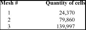
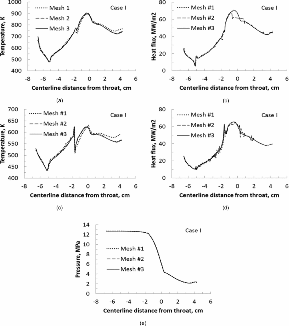
Initially, simulations were performed for Case I and tested for with each mesh resolution. Then, a total pressure and total temperature of inlet gas as well as mass flow rate and static temperature for inlet liquid (both segments) were specified. Figure 6 shows the gas-side and liquid-side wall temperature along the nozzle for the three meshes (6(a) and 6(c)), indicating good compliance between the results obtained with the Meshes #2 and #3. In addition, Fig. 6 also shows significant oscillations in heat flux distributions on Meshes #1 and #2 (6(b) and 6(d)) due to a poor mesh quality, which is overcome using Mesh #3. The down steps in the liquid-side temperature and heat flux at about 1.6 cm upstream from the throat result from the presence of the second segment inlet very close to the first segment outlet, in order to model the actual device where the cooling water is replaced in the cooling jacket just upstream from the nozzle throat. It is also possible to see the suitable agreement among the results obtained with the Meshes #1, #2, and #3, when the gas-side pressure is calculated along the nozzle (Fig. 6(e)), which means that all tested mesh reached sufficient resolution concerning this property.
Simulation results along the nozzle wall for different meshes: (a) gas-side temperature, (b) gas-side heat flux, (c) liquid-side temperature, (d) liquid-side heat flux, and (e) gas-side pressure.
The same procedures were repeated considering the remaining Cases II, III, and IV, and in all of them, results indicate the same behaviour. Based on this, it was possible to assure that Mesh #3 was appropriate for carrying out the numerical simulations.
7.0 RESULTS AND ANALYSIS
ANSYS Fluent(10) calculates the residual of an equation in two successive iterations and compares it with a user-specified value. If the residual is less than the user-specified value, that equation is deemed to have converged for the imposed boundary conditions. Such residual is based on the globally scaled residual defined as:
 $$\begin{equation*}
{R^\phi } = \frac{{\mathop \sum \nolimits_{cells\ P} \left| {\mathop \sum \nolimits_{nb} {a_{nb}}{\phi _{nb}} + b - {a_p}{\phi _P}} \right|}}{{\mathop \sum \nolimits_{cells\ P} \left| {{a_p}{\phi _P}} \right|}}
\end{equation*}$$
where ϕ is an evaluated parameter, anbϕnb + b represents the present solution, and aPϕP indicates the previous one.
Table 5 shows the results of globally scaled residuals of the governing equations for the last four iterations, considering each tested mesh for the Case I. Residuals of the continuity, x-velocity, y-velocity, z-velocity, energy, k, and ε equations presents an inconclusive behaviour comparing Meshes #1 and #2. However, all residuals decrease when comparing Meshes #2 and #3. It means the mesh refinement improves the convergence in the sense that meshes with higher resolutions decrease their influence on the simulation results. The same behaviour can be observed for the remaining Cases II, III, and IV.
Globally scaled residuals of each tested mesh for Case I
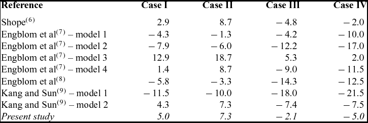
In order to evaluate the simulation results, Table 6 shows the deviation of the bulk temperature rise of the water in the second nozzle segment referred to in the experimental data obtained in the test facility HEAT H1, which was presented on a percentage base. It is possible to compare the simulation results calculated in the present study against those found by several authors that used the same experimental data and conclude that the results have excellent compliance. Simulations of the Cases I, III and IV presented deviations respectively of 5.0%, −2.1% and −5.0%, and the Case II presented deviation of 7.3%, all of them corresponding to a difference from the experimental data by at most 1.1 K. According to Shope(Reference Shope6), the nozzle for Case II has failed before the test reached the steady state, in which case the measured water temperature rise would be greater if the nozzle had survived, consequently reducing the deviation.
Deviation of the bulk temperature rise of the water in the second nozzle segment (%)
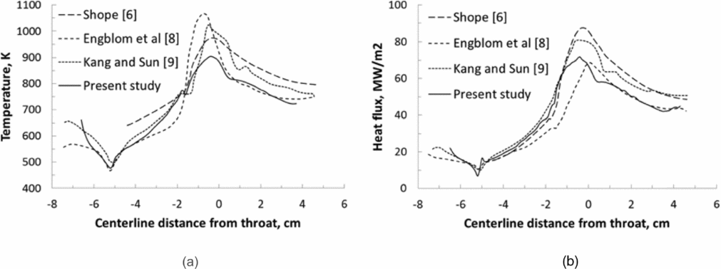
Figure 7 shows temperature and heat flux distributions along the gas-side nozzle wall provided by different authors in comparison with those obtained in present study. It can be observed that there is good compliance in the curves behavior with the peaks of temperature and heat flux occurring in the throat region. The small differences can be attributed to the mathematical modeling taken into account by each author.
Simulation results along the gas-side nozzle wall for case I: (a) temperature, (b) heat flux.
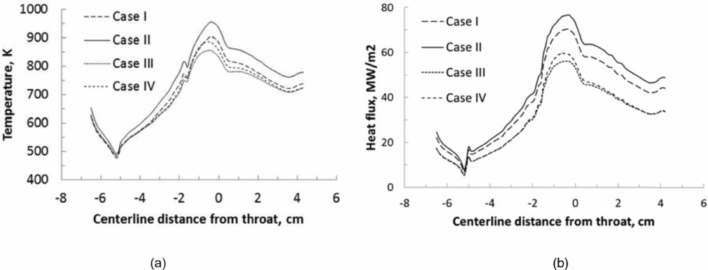
The heat transfer between gas flow and wall considers only forced convection, since radiation from the gaseous body to the wall is known to be about one order less than convection. In this sense, Fig. 8 shows heat transfer results at the gas-side wall in terms of temperature and heat flux profiles. Maximum values of temperature and heat flux are obtained in Case II, followed by Cases I, IV, and III. In all cases, the peaks of temperature and heat flux in the gas-side wall occur slightly upstream from the throat. Note the experimental data comprise two different sets distinguished by coolant mass flow rate, but with the same inlet temperature (see inlet conditions in Table 1). Indeed, accordingly to experimental data, simulations showed that the higher the air total enthalpy, the higher the gas-side wall temperature and heat flux, considering the same coolant mass flow rate.
Simulation results along the gas-side nozzle wall for Cases I to IV: (a) temperature; (b) heat flux.
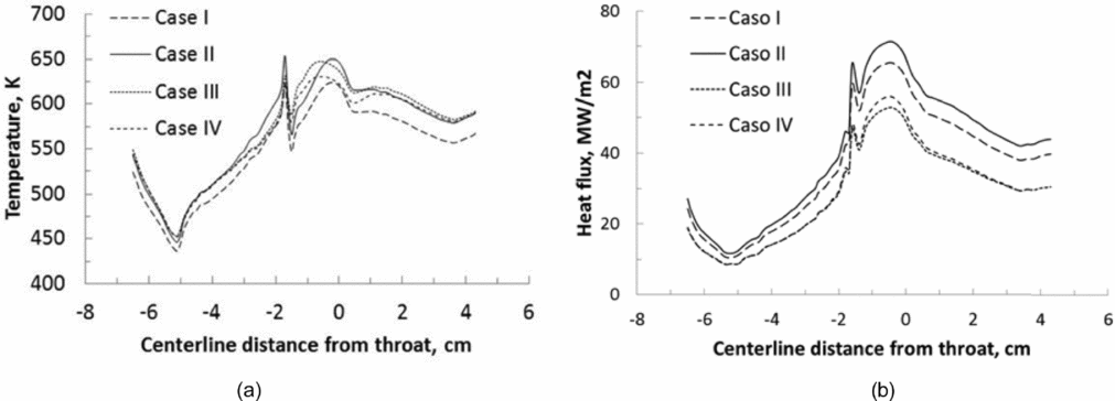
Figure 9 presents the results of interaction between inner wall and water flow (both segments) in terms of temperature and heat flux. The discontinuity at the vicinity of 1.6 cm upstream from the throat is related to the interruption of the cooling jacket between the first and second cooling segments, resulting in slight elevations of temperature and heat flux at the boarders of each cooling segments. In all cases, the peaks of temperature and heat flux in the liquid-side wall occur upstream from the throat.
Simulation results along the liquid-side nozzle wall for Cases I to IV: (a) temperature, (b) heat flux.
Comparing Figs 8 and 9, it can be observed that the liquid-side heat flux is less than the gas-side heat flux due to axisymmetric effects, since the water-side surface area is greater than the air-side area for a given length of conical frustum.
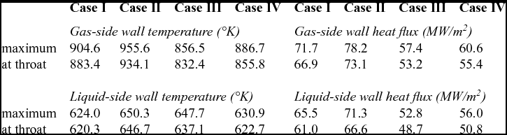
As mentioned above, the peaks of temperature and heat flux in both gas-side and liquid-side walls are found slightly upstream from the throat. In the Table 7, peak values of temperature and heat flux, as well as values at the throat are depicted for each case. Although the throat corresponds to the minimum passage area for the gas flow and leads to the maximum product value between density and velocity, it is known that local pressure also influences heat transfer by convection, justifying the displacement of the peaks upstream from the throat.
Gas-side and liquid-side wall temperature and heat flux at throat and maximum
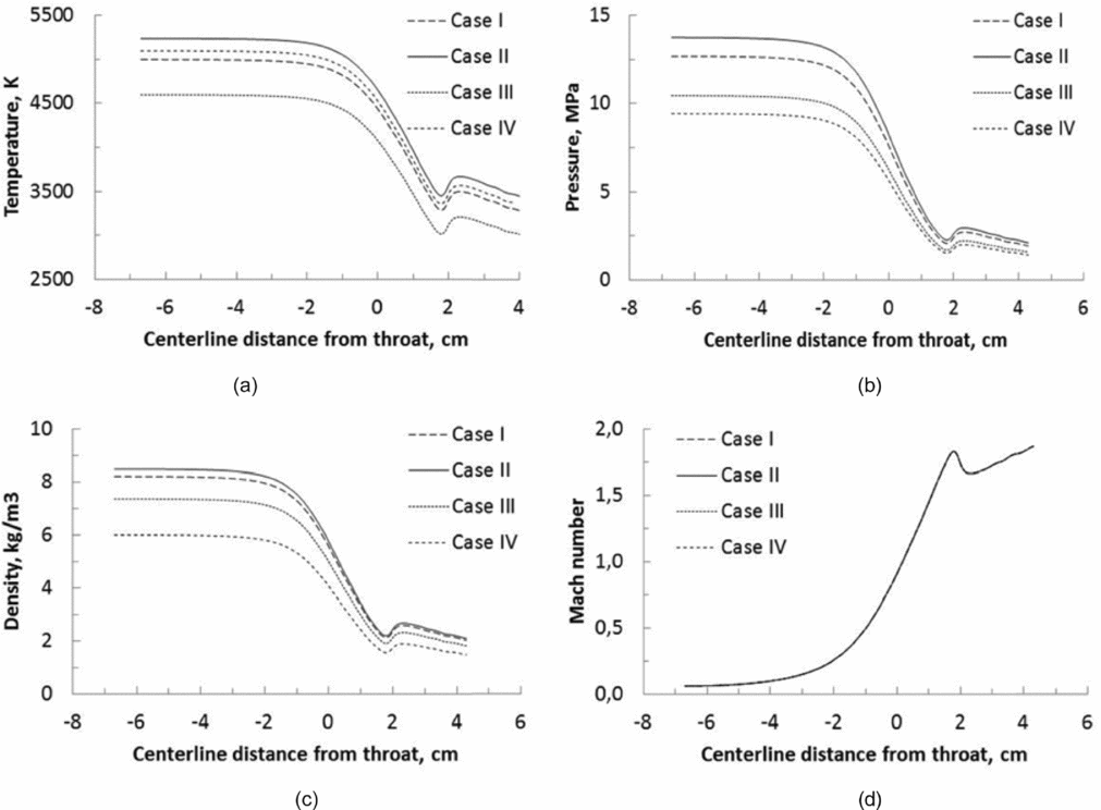
For the gas flow, Fig. 10 reveals a close link between temperature, pressure and density at the nozzle centerline, while values continuously decrease from the nozzle inlet up to a position 1.8 cm downstream from the throat, in opposition to Mach number behaviour. In this position, a small disturbance occurs and this fact can be better visualised further in this text. Also notable is the coincidence of the Mach number curves in all cases, demonstrating a behaviour compatible with ‘sonic’ or ‘shocked’ flow at the throat, which characterises the impossibility of increasing the gas flow velocity.
Simulation results along the nozzle centerline for Cases I to IV: (a) pressure, (b) temperature, (c) density, and (d) Mach number.
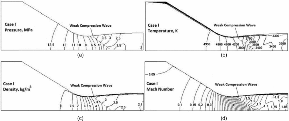
In order to extend the information about some parameters of the flow, Fig. 11 presents the iso-lines of temperature, pressure, density, and Mach number at a longitudinal section of the gas region only for the Case I, since Cases II to IV present the same behaviour. Pressure iso-lines (Fig. 11(a)) are orthogonal to the inner wall and the longitudinal axis due to the imposed null normal pressure gradient, meaning that the nozzle geometry has a significant effect on the pressure iso-lines curvature. Temperature iso-lines (Fig. 11(b)) also show that the normal temperature gradient strongly increases toward the nozzle wall, which can be observed by the iso-lines clustering, resulting in a high heat transfer rate. Density iso-lines (Fig. 11(c)) exhibit a moderate (strong) density variation in the convergent (divergent) nozzle section. In opposition to the temperature behaviour, the normal density gradient decreases toward the nozzle wall. The curvature of Mach iso-lines (Fig. 11(d)) progressively reverses departing from the nozzle inlet. It means that a comparison between Mach numbers near the core flow and those close to the wall showed higher values in the convergent region, equalised in the throat section, and lower in the divergent region.
Simulation results along the nozzle longitudinal plane for case I: (a) pressure, (b) temperature, (c) density, and (d) Mach number.
Also visible in these plots is the disturbance detected previously at the nozzle centerline. Here can be seen the tendency of disturbance propagation, which departs from the wall near the throat and achieves the centerline downstream from the throat. Such disturbance occurs due to the increase of the subsonic boundary-layer thickness near the nozzle throat that works as a constriction in the effective passage area, provoking the appearance of weak compression waves in the low Mach number supersonic flow.
8.0 CONCLUSIONS
A conjugate heat transfer problem considering gas-solid convection, solid conduction, and liquid-solid convection with an influence of sub-cooled boiling, is solved with the use of only one domain. This is the main advantage of this approach since it tends to save computational time and decrease intrinsic errors related to the iterations between combined domains. Results obtained by this unified approach showed good compliance with experimental data obtained at AECD test facility HEAT-H1 as well as computed results obtained by other approaches employed for the same problem.
Properties of dissociated air in thermodynamic equilibrium and properties of water (liquid and vapor) at constant pressure were used as temperature-dependent. Properties of Cu-Zr alloy were taken into account in the nozzle wall as a constant. Three meshes with different resolutions were generated to study the mesh sensitivity, considering four experimental cases distinguished by specific inlet conditions. In order to validate the model, the coolant bulk temperature rise in each experimental case and simulation results based in another approaches were compared.
Gas-side wall temperature and wall heat flux for all cases revealed similar behaviour, with peaks occurring slightly upstream from the throat. Analysis of the gas flow – particularly with respect to pressure, temperature, density, and Mach number distribution on the nozzle centerline – showed a disturbed region inside the flow, starting smoothly in the section between the first and the second cooling segments close to the wall. Such disturbance increases toward the core, reaching a peak downstream from the throat over the centerline.
Based on the results, it can be concluded that the unified approach presented in this study can be fully applied to the class of problems in which high-speed compressible flow and low-speed incompressible flow separated by a solid wall interact by means of conjugate convection-conduction process. Future improvements in this methodology could take into account aspects such as radiation from the gaseous body to the wall, reacting flow with chemical kinetics, and a more sophisticated sub-cooled boiling model based on multiphase flows.