

Introduction
One of the key stages of an Integrated Pest Management (IPM) system is the monitoring or continuous inspection of crops to ensure problems are detected early. Whereas in small fields operators can effectively perform this surveillance, in large areas, sampling at certain selected points is currently the only viable monitoring option. Therefore, the development of technologies that enable the automatic and continuous on-ground inspection of crop fields is of great interest. Among the various means of collecting well-structured information is the use of reasonably priced, autonomous vehicles equipped with on board sensing equipment, which are considered to be one of the most promising technologies in the medium-term. However, the use of mobile robots in agricultural environments remains challenging as navigation in agricultural environments presents difficulties because of the variability and nature of the terrain and vegetation. Bechar and Vigneault (Reference Bechar and Vigneault2016) presented a current review of developments and innovation in agricultural robots for field operations, analysing their main limitations.
The use of medium-size robots for fully inspecting a crop is a suitable choice to minimise the soil compaction and it is the only way to safely travel across woody crops. Therefore, it can be a useful option for early pest detection by gathering the geo-referenced information needed to construct accurate crop maps. Furthermore, more than one sampling can be performed throughout the year because of the minimal impact on the crop.
In the following sections, an inspection system is presented as well as its initial performance results. The developed inspection system is composed of 1) a multisensory and autonomous inspection platform integrated on a commercial vehicle able to fully cover a field following a predefined route (Conesa-Muñoz et al., Reference Conesa-Muñoz, Bengochea-Guevara, Andújar and Ribeiro2016) and able to collect geo-referenced information, hereafter named the field platform; and 2) custom software developed to automatically generate the 3D crop reconstruction as well as the map of the crop volume distribution from the heterogeneous information acquired in the field, hereafter named the 3D mapping module.
Materials and methods
Field platform
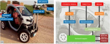
The field platform (Figure 1a) is based on a Twizy (Renault), which has a 13 kW (17 hp) electric motor and is able to travel up to 80 kmh−1 (50 mph). The vehicle has range of approximately 80 km after a 3.5-hour charge using a standard plug. The field platform is an ultra-compact vehicle, with a length of 2.32 metres, width of 1.19 metres and height of 1.46 metres. The electric motor of the vehicle allows vibration free speeds below 3 kmh−1, which is convenient for high-quality information acquisition.
(a) Field platform based on a Twizy vehicle from Renault. (b) Developed control architecture.

An aluminium support structure has been integrated for easy placement of sensors. Two cameras were integrated, adapting their positions to the crop features of each sampling. The first camera is an RGB-D sensor (Kinect v2, Microsoft), which supplies, at 30 fps, RGB images with a resolution of 1920×1080 pixels together with depth information with a resolution of 512×424 pixels. Depth data are obtained by using ToF (time-of-flight) technology. The second camera is a reflex camera (EOS 7D, Canon), which, at 2 fps, supplies high-quality RGB images with a resolution of 2592×1728 pixels. Both cameras were connected to the on-board computer, which has an Intel Core i7-4771@3.5 GHz processor, 16 GB of RAM, and an NVIDIA GeForce GTX 660 graphic card. The inspection vehicle is equipped with an RTK-GPS receiver (R220, Hemisphere), which provides location data at 20 Hz sample rate with an error below 2 cm.
The on-board computer is responsible for the decision-making processes, sending the commands to the vehicle when it is either working in remote control mode, autonomously based on RTK-GNSS receiver information or on-board sensors information. Thus, the hardware concept architecture (Figure 1b) was developed to manage the speed and the turning of the vehicle; in other words, to control the acceleration, braking and steering systems. The automation of the vehicle was performed focusing on the brake and accelerator pedals to keep the manual driving mode. Note that the used platform is a registered vehicle that can be driven by road, if needed.
The vehicle’s power inverter controls the motor speed by producing variable output voltage that references the accelerator pedal position. The system is specifically composed by two potentiometers whose resistances vary with the pedal position. Consequently, for automatically performing the speed change commands sent by the on-board computer, a stepper motor and a microstep controller have been integrated for increasing the number of steps per full rotation up to 6 400. The motor is connected to an Arduino board, which generates the signals to the internal motor controller of the vehicle. The objective is to simulate the pressure on the accelerator pedal. In contrast to the acceleration system, both the steering and braking systems are completely mechanical; thus, the automation requires the use of some actuator. In the case of the steering system, a DC motor connected to an encoder directly managed by a position controller was integrated. The position controller allows control of the vehicle direction by continuously handling the steering wheel position as well as its rotation speed. Finally, for the braking system, a servomotor connected to the brake pedal through a strong wire was included. The stop commands sent by the on-board computer reach the servomotor through the Arduino board.
The on-board computer interprets the decisions to control the vehicle by using fuzzy control techniques. Several previous works (Fraichard and Garnier, Reference Fraichard and Garnier2001, Kodagoda et al., Reference Kodagoda, Wijesoma and Teoh2002, Naranjo et al., Reference Naranjo, Sotelo, Gonzalez, Garcia and Sotelo2007, Bengochea-Guevara et al., Reference Bengochea-Guevara, Conesa-Muñoz, Andújar and Ribeiro2016) have showed that fuzzy controllers perfectly mimic human driving behaviour while driving and route tracking. Thus, they help manage the nonlinear dynamics that characterises the wheeled mobile robots, usually affected by an important number of disturbances, such as turning and static frictions or variations in the amount of cargo. Human behaviour regarding speed and steering control can be approached using artificial intelligence techniques, among which the techniques based on fuzzy logic (Zadeh, Reference Zadeh1965; Sugeno, Reference Sugeno1999) provide a better approximation to human reasoning, giving a more intuitive control structure.
3D Mapping module
To properly monitor woody crop status, it is essential to estimate some geometric features of trees such as its height and the canopy volume. Indeed, canopy volume allows, among others, the analysis of the tree production capacity and the optimization of a number of agronomic tasks, such as water use, nutrient application and pruning operations. Even more, geometric features can be essential in the early pest detection, since changes on the expected states of height or canopy volume may point to the existence of some emerging disease.
Usually, tree dimensions are measured by hand at field, a really tedious job. Then the canopy envelope is approaching to a regular polygon to estimate its volume or empiric models are applied.
The mapping process developed is fully automatic and is composed of the following steps per woody row: 1) generating the point cloud, 2) splitting the point cloud into same-length sections, 3) changing the coordinate system of each section and 4) extracting the canopy from the point cloud in each section. Once this point is reached, an accurate 3D representation of the crop row is available where different parts of the trees are identified. Furthermore, data are prepared to build volume maps among others tasks.
The point cloud (first step) is generated by the fusion of different overlapped depth images using a method based on the algorithm described in (Niessner et al., Reference Niessner, Zollhöfer, Izadi and Stamminger2013). The algorithm, selected for its good results in the point cloud generation of large areas, overcomes the issues of other methods (Chen et al., Reference Chen, Bautembach and Izadi2013, Steinbrucker et al., Reference Steinbrucker, Kerl and Cremers2013, Whelan et al., Reference Whelan, Kaess, Fallon, Johannsson, Leonard and McDonald2012) including the Microsoft software (Newcombe, 2011), which only manages volumes up 8 cubic metres, thus imposing an important constraint for agricultural contexts. In addition, a variant of the Iterative Closest Point (ICP) algorithm (Chen and Medioni, Reference Chen and Medioni1992) was integrated to improve the precision of the point cloud obtained in an attempt to reduce the drift in the reconstruction. The depth information is fused to the current model using a weighted moving average while the RGB information is also updated using an exponential moving average.
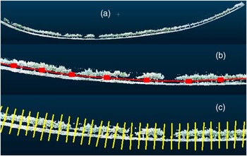
The point cloud obtained represents a woody row, but it does not appear to be as straight as the original due to the drift effect (Figure 2a), which makes the canopy volume estimation difficult because the point cloud is not easy to divide into smaller same-length pieces. The second and third steps were developed to properly handle the drift drawback. The second step divides the whole point cloud into smaller clouds with the same number of points and then calculates the centroid for each of these point clouds (Figure 2b). Note that although each cloud contains the same number of points, it does not represent the same length of the woody row because the point distribution in the whole cloud is not uniform. Thus, more pieces divide the whole cloud, more centroids are obtained and a more precise fit to the woody row is achieved. The number of pieces of smaller clouds may be estimated from the row total length. Next, the line that joins all the centroids (model line) is built and used to divide the initial point cloud into same-length sections separated by planes perpendicular to the line in each separating point (Figure 2c). The segment length must be fixed according to the required resolution in the final map. Note that shorter segments result in a more accurate map. The points contained in each section hereafter are named the section cloud.
(a) Original crop row. (b) Model line by using points. Note that the points are not equidistant (c) Crop row divided into 1-m length sections. Note that all sections have the same length.

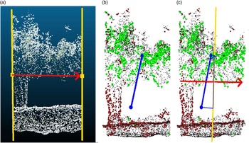
Because the drift may completely twist the crop row in any direction, it is necessary to straighten each section according to coherent axes. In other words, assignment of the lowest z-levels to the ground and higher z-levels to the tree canopy or higher tree parts and then alignment of the section width (x-axis) with the direction of the woody crop and the section depth (y-axis) perpendicular to the same direction must occur. The third step applies a transformation matrix to the points contained of each section. The matrix is composed of the vectors that determine the new coordinate system (new axes), setting the origin in the section centroid with regard to the old coordinate system. The direction of the x-axis is calculated using a normalised vector that connects the starting and ending segment points where the section is contained (Figure 3a). The z-axis, which should indicate the height direction, is determined in two steps. Initially, the greenest points are selected from the cloud by combining (Burgos-Artizzu et al., Reference Burgos-Artizzu, Ribeiro, Tellaeche, Pajares and Fernández-Quintanilla2010) the RGB values of each point into a single value in the 0–255 range, where the more likely the point is contained in the green layer, the higher the value is. The 10% highest value points are used to calculate the top centroid; similarly, the bottom centroid is calculated by using only the 10% lowest values. Figure 3b shows the 10% of the highest values in grey and the 10% of the lowest values in black. Moreover, the top and bottom centroids are plotted as well as the line that connects them. To obtain the z-axis direction, an orthogonal plane to the x-axis is calculated that also contains the midpoint of the section in the x-axis. Next, the bottom and top centroids are projected onto this plane (Figure 3c) and the vector that connects them is orthogonal to the x-axis and, once normalised, defines the z-axis direction.
(a) Vector that defines the x-axis direction. (b) Point cloud of the section with the 10% of the highest values represented in grey and the 10% of the lowest values in black. The top and bottom centroids are plotted. (c) Projection of the segment joining the top and bottom centroids onto an orthogonal plane to the x-axis that contains the midpoint of the section in the x-axis.

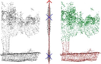
Once the points coordinates are transformed, the section is aligned with the z-axis, i.e., the ground is on the bottom and the canopy is on the top. Points in the section appear divided into two point clouds, canopy and ground, separated by a thinner and much smaller cloud of points belonging to the trunk. Next, considering only the z component of the points, because there is a clear middle-gap in that component, the k-means algorithm (Mcqueen, 1967) is employed to extract the two clusters, where points in the top cluster belong to the tree canopy (Figure 4). At this point, a 3D representation of the whole woody row is available, identifying the tree canopy from the rest.
Section cloud points projected onto z-axis and classified in two clusters. The crosses show the cluster centroids.

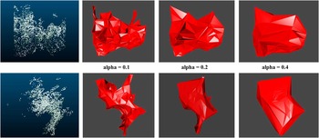
To estimate volumes, first, an alpha shape (Edelsbrunner and Mucke, Reference Edelsbrunner and Mücke1994) or volume that envelops the set of 3D points must be obtained. The alpha parameter specifies how tight the body fits the points. There are many software libraries to address this issue. In the developed system, the R alphashape3d package (Alphashape3d package, 2016) based on the original Edelsbrunner and Mucke’s work is used. Figure 5 shows different alpha shapes according to the alpha value selected for the same point cloud (front and side view). Higher values showed very loose shapes, whereas lower values generated very tight bodies. An alpha value of 0.2 was selected. Finally, the same function library that allows calculation of the alpha shapes, allows also estimation of the volume.
Alpha shapes for the same point cloud (part of a tree canopy). The first row corresponds to the front view and the second row corresponds to the side view.

Finally, the volume map is built as the union of the volume maps of all sampled rows. To obtain the volume map of a row, the volume value of each section is projected onto the segment joining the start and end points (GNSS locations) of the row.
Results and discussion
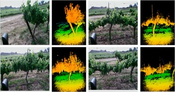
Several tests were conducted in 2016 in the vineyards owned by Codorniu S.A. (Raimat, Lleida, Spain). Figure 6 shows examples of the information provided by Kinect v2 sensor in the vineyard in the sample conducted in February. The sensor was mounted at approximately 1.4 m in height and approximately 1 m from the crop row. Figure 3a shows the RGB information of the scene, and Figure 3b shows a colour representation of the depth information (distance of objects in the scene), where near objects appear in red and further ones in blue, and the rest of the intermediate objects are shown in various shades of orange, yellow and green, depending on their distance from the sensor (see digital version of the paper to appreciate the colour range). From the depth images, it can be seen that the Kinect range of operation meets the inspection requirements of the vineyard rows because objects of no interest very close are ignored as well as the distant areas that usually contain others vineyard rows.
Several RGB images and depth images given by the Kinect v2 sensor.

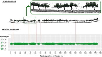
Figure 7 shows the results of the developed inspection system and the 3D mapping module in particular. Thus, the reconstruction of one of the vineyard rows sampled during the February campaign as well as the distribution of estimated volumes for the row is displayed. Note that reconstruction and volume values were obtained from data acquired by scanning only one side of the vineyard row. Therefore, the volume values may be underestimated, although in woody crops with narrow rows, such as the current one, the correlation between estimated volume and actual volume is assumed to be high. In addition, the 3D reconstruction and the volume distribution appear to consistently match; for example, lower volume values appear in those points where the 3D reconstruction shows no vineyard and the higher volume values are generally presented in the more leafy zones.
Results for the 3D mapping module. 3D reconstruction and volume distribution for a sampled vineyard row.

Conclusions
This paper describes an inspection system designed and developed to autonomously scout crops. The inspection system is composed of an autonomous inspection mobile platform based on a commercial electric vehicle and custom software was prepared that is capable of scanning two types of scenarios: annual crops (maize, cereal, etc.) and multi-annual crops (orchards, vineyards, etc.). The preliminary tests conducted during 2016 demonstrated proper vehicle operation, including the on-board sensors, based on the sampling results of actual crop fields. Furthermore, the performance of the developed software was tested with good results in the automatic 3D reconstruction of vineyard crops as well as in the automatic generation of canopy volume distribution maps. The technology presented in this paper is particularly important for implementation of crop management consistent with the precepts of an Integrated Pest Management system. Finally, it can be concluded from the preliminary results that the proposed inspection system could become a viable alternative to UAV-based inspection and, in any case, is a complementary technology to aerial and satellite options.
Acknowledgements
This project is funded by the Spanish Government (AGL2014-52465-C4-3-R). The authors thank Jordi Recasens and his team (Weed Science and Plant Ecology Research Group of the UdL) for their invaluable help in the field trials. The authors acknowledge the invaluable technical support of Damián Rodríguez.