Introduction

The recent shifts in research from the investigation of regional features to climate change and long-term variability in the global atmosphere-ocean-land coupled system have initiated intensive developments in large-scale ocean modelling. The polar oceans are an important part of the global climate system and therefore need to be fully understood before we can have confidence in predictions of rapid climate change. However, because of the small Rossby radius in the Arctic Ocean, ocean models covering the region need to use a grid of much less than 10 km in order to fully resolve the mesoscale features. The present model has sufficient resolution to permit some mesoscale activity and will start to resolve currents and eddies larger than 30 km, providing new insights into the Arctic circulation. Recent improvements in computer power have made such models practical.

Description of the Model and Model Runs

The Ocean Circulation and Climate Advanced Modelling project (OCCAM) model is a level model based on the Bryan-Semtner-Cox "primitive"equations for the ocean. Potential temperature, salinity, surface height and components of the velocity are the prognostic variables which describe the dynamical and thermodynamical states of the ocean. Several enhancements of the original Bryan-Semtner-Cox model were made in order to improve its performance (Webb and others, unpublished). The "rigid-lid" approximation used in the original model was abandoned and a simple tidal model was used to solve the barotropic equations. The second major development includes the introduction of a new advection scheme, termed the Split-QUICK scheme (Reference Webb, de Cuevas and RichmondWebb and others, 1998). This is based on Leonard’s QUICK scheme (Leonard, 1979) but splits the operator into pure diffusive and advective parts. The model uses Pakanowski and Philander mixing for the tracer fields, although at high latitudes the vertical diffusion coefficient reverts to its constant background value of 0.5 cm² s ⁻¹ . To obtain a fully global coverage, and to overcome the convergence of the meridians near the poles, two spherical grids were used. The first is a standard latitude-longitude grid covering the South Atlantic, Pacific and Indian Oceans. The second grid, which is rotated so that its "north" pole lies on the geographical equator, covers the North Atlantic and Arctic Oceans. The two grids are fully coupled along the Atlantic equator, and a channel model is used to provide a connection through the Bering Strait. The channel model balances the pressure difference between the Pacific and Arctic ends of the strait by bottom friction in a channel of uniform width (60 km), length (30 km) and depth (20 m). The pressure difference is determined by the prognostic sea-surface heights at each end of the strait. The horizontal resolution in the Arctic Ocean and Nordic seas is about 27 and 14 km for 1/4° × 1/4° and 1/8° × 1/8° resolutions, respectively. The model uses an Arakawa-B grid because of its better performance in representing the propagation of short Rossby waves and fronts. The model has 36 levels in the vertical, varying in thickness from 20 m near the surface to 250 m at depth. The 1/12° DBDB5 dataset was used to derive the seabed topography. Finally, it is worth adding that the structure of the model code was changed in order to be run efficiently on array processor computers using message passing (Reference WebbWebb, 2000; Webb and others, unpublished).

Both the 1/4° and 1/8° models were forced with a monthly climatological surface stress (European Centre for Medium-range Weather Forecasts) calculated from data for the period 1986−88. The resulting set of 12 monthly, mean wind-stress fields was applied repeatedly for each model year of integration. The present versions do not include explicit treatments of sea ice, river runoff or atmospheric fluxes of heat and fresh water. Instead both models were "relaxed" to monthly mean climatological temperature and salinity fields (Reference Levitus, Boyer and AtonovLevitus and others, 1994a, Reference Levitus, Burgett and Boyerb) with a relaxation time-scale of 30 days. Rather than applying a virtual salt flux, the salinity difference was used to derive a fresh-water flux which could affect the sea-surface height and hence the volume of the surface box. The annual mean p-e difference which results from this process is shown in Figure 1. The values do not exceed ±6.3 m a⁻¹. High values correlate with areas of river water inflow, and low values with regions of regular ice production (e.g. the Novo Sibirskaya Polynia).

Fig. 1.

Annual mean P− E difference (m a−1) in the arctic ocean for the 1/4° model. the 0 isoline is shown in bold.

The initial state of the 1/4° model was prescribed by Levitus’ climatology (Reference LevitusLevitus, 1982). For the first 6 months of integration, temperature and salinity were relaxed to this climatology with a time-scale of 30 days at the surface and 360 days for all other levels. After 6 months the climatology was replaced with Levitus’ climatology (Reference Levitus, Boyer and AtonovLevitus and others, 1994a, Reference Levitus, Burgett and Boyerb), and the model integrated for a further 3.5 years. After year 4.0, integration continued with surface relaxation only. The model state of year 8.0 of the 1/4° model was used to derive the initial state of the 1/8° model which was integrated forward for two model years using surface relaxation only.

Analysis was carried out on both instantaneous and time-averaged fields. We used model results from a 4 year period of the 1/4° model (year 8.0−12.0) which comprised full-depth instantaneous fields every 15 days and instantaneous surface fields every 2 days. Results from the second year of the 1/8° model integration, comprising full-depth instantaneous fields every 10 model days, instantaneous surface fields every 5 days and their averages, were employed.

Clearly neither model will have reached an equilibrium state within the analysis period. However, diagnostics, such as the global averaged kinetic energy, temperature change and salinity change, suggest that the circulation patterns are generally established during a 6 month adjustment phase followed by a slow "drift" towards an equilibrium state. We consider that the results from the analysis period give a detailed and coherent view of a possible circulation structure which can be supported by much of the observational data for this area.

Large-Scale Ocean Circulation and Water Masses

Because the model is strongly relaxing to Levitus chmatological temperature and salinity at the surface, it should not drift very far from the climatology within the integration periods presented. Therefore, comparison between simulated and climatological temperature and salinity fields should confirm that the model has remained close to the present climate. Most new insights are likely to come from analysis of the circulation structure. We have compared simulated hydrographic fields to several sources of observations (e.g. Reference TimofeevTimofeev, 1961; Reference McLaughlin, Carmack, Macdonald and BishopMcLaughlin and others, 1996; NSIDC, 1997). The NSIDC data are derived from Russian archive data not used for Reference Levitus, Boyer and AtonovLevitus (1994a, Reference Levitus, Burgett and Boyerb) and show the presence of many fine-scale features similar to the model. A detailed comparison is beyond the scope of this paper, but, generally speaking, good agreement was found between model and hydrographic profiles at selected locations around the Arctic basin.

The model results show a self-consistent picture of the Arctic Ocean Circulation, reproducing the following large-scale circulation features observed in the Arctic.

Flow Through the Arctic Straits

As the first level of validation we consider water transport through the major straits which connect the Arctic Ocean to the World Ocean, and compare these model estimates to the known fluxes. The following five main channels were selected: Bering and Fram Straits, Barents Trough, Nares Strait (which separates Greenland and Ellesmere Island) and Lancaster Sound (eastern part of the Barrow Strait). Narrower straits are not resolved by either version of the model. In addition, the flux through the meridional section located immediately north of Ellesmere Island was calculated in order to check the strength and variability of the boundary current near the Greenland Shelf. For the 1/4° model the Nares Strait is closed, so the water from the Arctic Ocean can enter the North Atlantic only via the Barrow Strait. As will be shown later, this significantly affects the magnitude of the water transport through the Canadian Arctic.

The water transport through the Bering Strait is one of the best defined from observations. These show that the net transport in the strait is always directed towards the north and leads to the permanent inflow of the Pacific Water into the Chukchi Sea. The mean annual flux is about 0.8−1.2 Sv with variance of 0.2−0.5 Sv (Table 1). The transport has a strong seasonal variability, with a maximum of about 1.3−1.9 Sv in June-August and minimum of around 0.3−0.6 Sv in February −March (Reference Coachman and AagaardCoachman and Aagaard, 1988; Reference RoachRoach and others, 1995). A secondary maximum of the transport, with a net flux of about 0.8 Sv, was observed in October-December.

Table 1.

Simulated and observed water transports (Sv) though the arctic straits

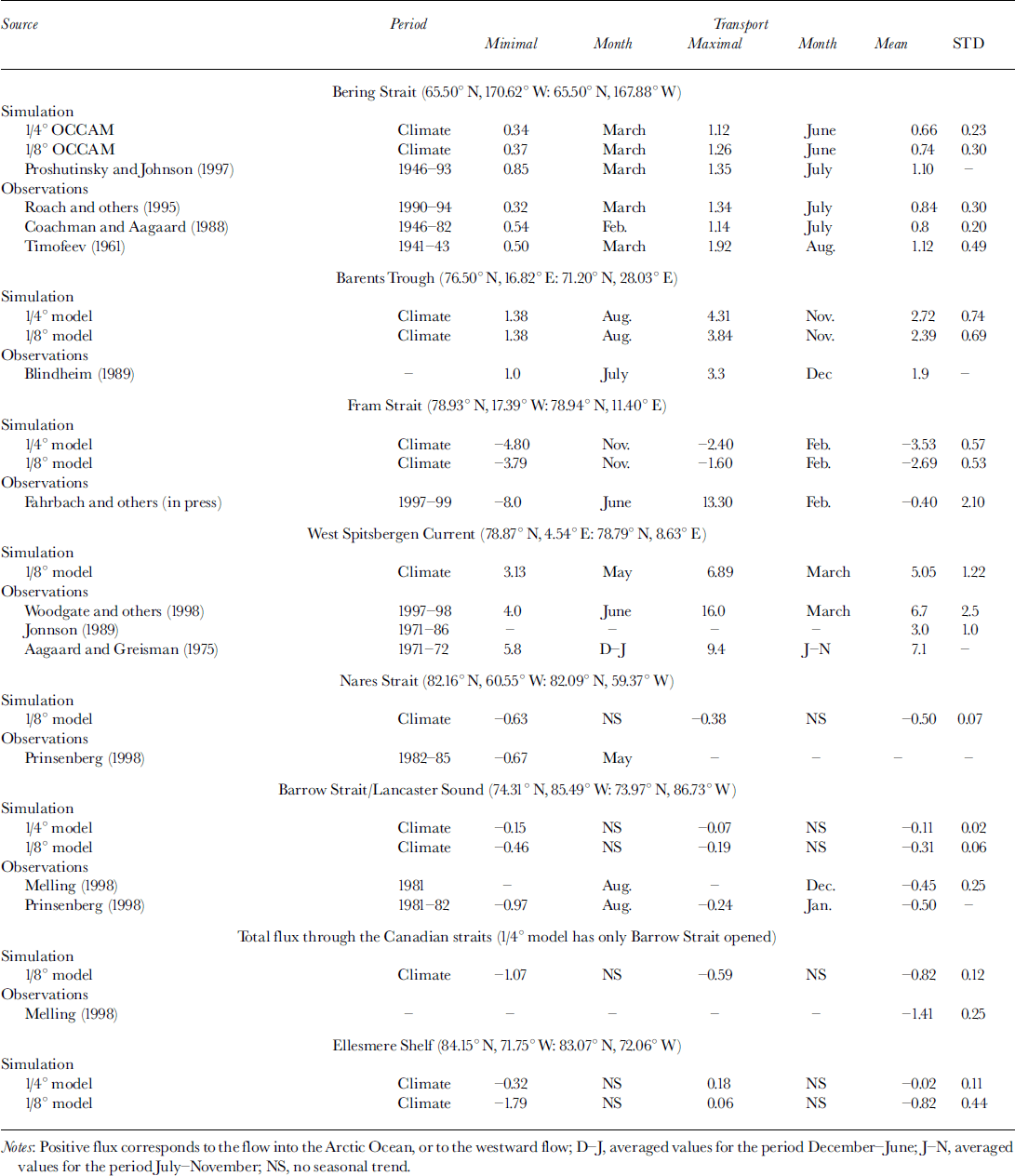
The model results exhibit a seasonal variation of the volume flux through the strait similar to the observed one (Fig. 7a). According to the 1/8° model results, the simulated volume flux varies from 0.37 Sv in March to 1.26 Sv injune. The 1/4° model gives very similar figures: 0.34 Sv in March and 1.12Sv in June. Both models display evidence of the existence of a secondary maximum (0.65 and 0.76 Sv for the 1/4° and 1/8° versions, respectively) in December-February (Fig. 7a). As the graph clearly shows, the coincidence of the observed (Reference RoachRoach and others, 1995) and simulated transports in the Bering Strait is remarkable. Other ocean models employed for the same region show similar volume net flux variability (Table 1; or see, e.g., Reference Proshutinsky and JohnsonProshutinsky and Johnson, 1997).

Fig. 7.

Simulated water transport through the bering strait (a), fram strait (b), barents trough (c) and canadian straits (d). the results from the 1/4° model (dashed lines) and 1/8° model (solid lines) and observations for the bering strait (dash-dotted lines) are shown. northward and eastward fluxes are positive.

Transport through the Fram Strait has a major impact on the Arctic Ocean circulation. The strait is about 500 km wide at the narrowest part, with a sill depth of about 2500 m. It is sufficiently large to house a complex circulation structure. Thus the flux in the Fram Strait is not easy to estimate from observations because of the intricate topography and pattern of currents. Two major streams, the northward-flowing WSC and the southward-flowing EGC, pass through the strait. The WSC branches in the northern part of the strait and loops westward to form a southward counter-current which joins the peripheral part of the EGC. Estimates of the monthly mean volume transports by these two main streams are 3−10.8 Sv for the WSC and 3−11.2 Sv for the EGC (Table 1). Despite the large fluxes, the net transport through the strait is thought to be about 1−3 Sv towards the Atlantic. At present, the question of whether or not the net flux through the strait has significant seasonal variability is still open, but recent long-term current measurements seem to support this hypothesis (Reference Woodgate, Schauer and FahrbachWoodgate and others, 1998). It is believed that the presence of several branches of the WSC and its overall instability can substantially obscure the seasonal signal in the water transport.

Comparison between the volume fluxes calculated from the available current-meter observations and from the model shows that the observed fluxes exhibit greater variability than model ones, but the observed mean net flux is actually smaller. The difference could be attributed to the method used for calculating fluxes from this set of current-meter measurements. Most of the measurements were performed in the western or central part of the strait and did not include the shelf part of the EGC. Therefore the mean outflow from the Arctic Ocean may well be underestimated. This can also affect the flux variability, increasing the range of calculated transports. Both 1/4° and 1/8° models give a net volume transport to the south of about 3.5 and 2.7 Sv, respectively, with average fluctuations of about 0.5 Sv (Table 1). Besides the obvious seasonal variability the quasi- periodical oscillations with a period of about 50 days are present from February to August (Fig. 7b). We calculated the transport time series for the sections crossing the strait at 76.6° N, 79° N, 79.8° N, and found such oscillations in all of them. One can hypothezise that the fluctuations could be related to short-period variability in the recirculation between the WSC and EGC or to local wind conditions, but the origin of these oscillations is not yet fully understood. A similar type of variability can be found in the observations (Fahrbach, in press).

We performed a comparison of the simulated and observed water transport within the WSC (Table 1). The average flux for the period October-June calculated from the results of the 1/8° model (5.37 Sv) is lower than that recently observed (6.7 Sv) during the Variability of Exchange in the Nordic Sea (VEINS) experiment (Fig. 8). However, the simulated transport is in reasonable agreement with other estimations (3−7 Sv) made from observations taken during the last 20 years (see Reference Woodgate, Schauer and FahrbachWoodgate and others, 1998, for an overview of past observations).

Fig. 8.

Water transport within the wsc the simulated monthly mean transport from the 1/8° model (solid lines) and observations (dash-dotted lines) from Reference Woodgate, Schauer and Fahrbachwoodgate and others (1998) together with their error limits (dashed lines) are shown. northward and eastward fluxes are positive.

Transport through the Barents Trough is an important part of the water exchange between the Nordic seas and the Arctic. Simulations give values of 2.39 and 2.72 Sv for the 1/8° and 1/4° models, respectively (Table 1). Weak seasonal variability of the flux is presented and is in the opposite phase to the transport through the Fram Strait (Fig. 7b and c).

According to recent publications, the water flux through the Canadian Archipelago is the same order of magnitude as the net flux through the Fram Strait (Reference Melling, Aagaard, Hartmann, Kattsov, Martinson, Stewart and WeaverMelling, 1998; Reference Prinsenberg, Aagaard, Hartmann, Kattsov, Martinson, Stewart and WeaverPrinsenberg, 1998). The published figures for the mean annual transport from the Arctic Ocean to the Labrador Sea are 0.7−1.7 Sv.

Most coarse-resolution models cannot resolve the relatively narrow and shallow channels between the islands of the Canadian Arctic. In our 1/4° version the Arctic Water enters the Labrador Sea via Lancaster Sound (eastern part of the Barrow Strait) only. The 1/8° model has the Nares Strait opened in addition, and allows 0.5 Sv of the Arctic Water to pass through the passage into the Labrador Sea. The total volume flux from the Arctic Ocean into the Labrador Sea according to the 1/8° model is about 0.8 Sv, which is close to the estimation made by Reference Melling, Aagaard, Hartmann, Kattsov, Martinson, Stewart and WeaverMelling (1997). However, the seasonal structure of the transport variability calculated from the available current observations is different from that simulated in the model (Table 1). The simulated transport (1/4° model) through the Lancaster Sound does not show any significant seasonal variability, with the maximum in October and minimum in June, whereas the transport calculated from the current measurements and hydrographic observations has a minimum in December and a maximum in August (Table 1). Leaving aside the model errors, we would like to emphasize that the seasonal curve proposed by Reference Prinsenberg, Aagaard, Hartmann, Kattsov, Martinson, Stewart and WeaverPrinsenberg (1998) is based on single-point year-long current measurements. They in their turn were correlated to the across-strait section completed in April 1982. On the other hand, the absence of an explicit treatment of sea ice in the model, together with the unavoidable coarsening of the topography, leads to an underestimation of the currents in the narrow straits. The model flux has short-period variability over a period of about 70−100 days, very similar to that obtained in the Fram Strait. In the 1/8° model the oscillations are easily noticeable in the Lancaster Sound time series, and completely overwhelm the seasonal signal in the Nares Strait. To understand whether these oscillations are caused by the oscillations of the current on the Canadian Shelf, we analyzed the volume transport from both models through a section across the shelf immediately north of Ellesmere Island. None of the periodic component was found, but rather the signal exhibits chaotic fluctuations. Quarter-degree model results show quasi-periodical variations in the transport but with the Nares Strait closed.

As one can see from Figure 7, the model resolution significantly alters the water transport through the Fram Strait and the Canadian Arctic. By opening the Nares Strait in the 1/8° model we increased the export of water from the Arctic into the Labrador Sea by almost a factor of seven, when the mean annual flux through the Fram Strait dropped by 25% (Table 1). The resolution had little effect on the water influx through the Bering Strait and Barents Trough (Fig. 7a and c).

Concluding Remarks

The main weaknesses of the present model versions are obvious: simplified treatment of the sea-ice evolution and too short an integration period. Despite these weaknesses, the model reproduces realistic and coherent simulations of the Arctic currents and water-mass properties. We would argue that the high-resolution ocean general-circulation model presented here is a very powerful tool for studying both large- and small-scale features in the Arctic. It can also help us to investigate the longer-period variability of the ocean circulation incorporating the correct physics of the small-scale processes.

The great advantage of high-resolution models is in resolving fine-scale structures approaching the order of the Rossby scale or less. One class of such features is small-scale eddies, which are involved in the transport of kinetic energy from the boundary of the Arctic basin into its interior. Other examples of fine structure are the narrow (≤100km wide) eastward boundary currents localized on the continental-shelf slope and literally encircling the entire Arctic Ocean. We have discussed these boundary currents in some detail and shown that they are consistent with hypotheses based on limited observations. However, within the model we also find narrow jets not only near the shelf break but also in the interior of the ocean. Unexpectedly the whole basin is "packed" with these features, in contrast to the shallow waters of the Siberian Shelf. Observing these features will present a significant challenge for future hydrographic programs.

Concerning the future, several model improvements are underway. The first is to couple the ocean model to a sea-ice model. The elastic-viscous-plastic model developed by Hunke (Reference Hunke and DukowiczHunke and Dukowicz, 1997) will be used. This model has a well-tested viscous-plastic rheology, and its fully explicit numerical scheme is efficient for parallel architectures. We hope to maintain the computational efficiency obtained with the current model and thus achieve longer integration periods without having to compromise further on model resolution.