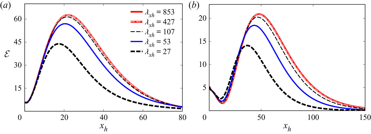
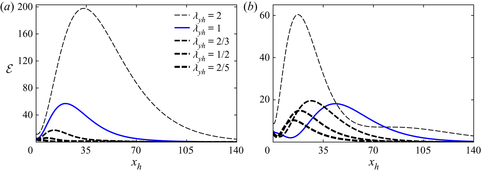
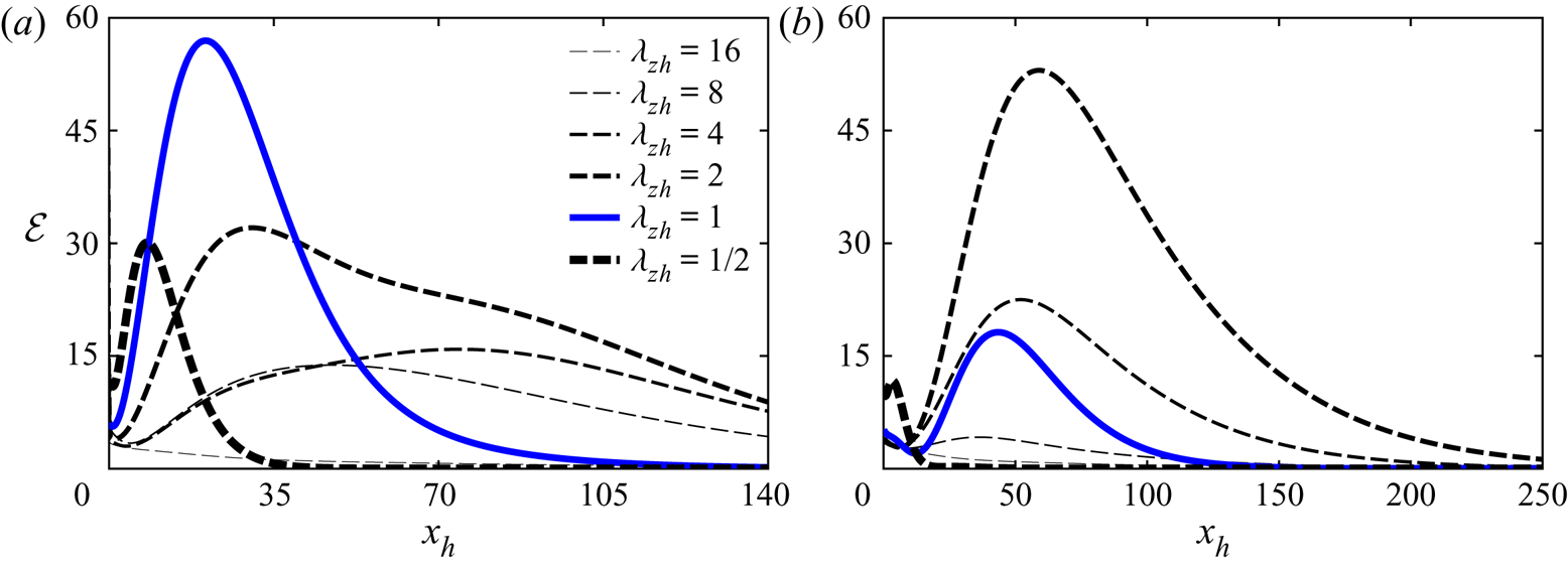
1. Introduction
Laminar-to-turbulent transition is a phenomenon that has puzzled scientists since the pioneering experimental work of Reynolds (Reference Reynolds1883). Even in the simplest geometries, it is often not completely clear how the laminar flow becomes unstable and breaks down to turbulence. For example, all theoretical and numerical works show that laminar pipe and Couette flows are always linearly stable at every Reynolds number, whereas obviously turbulence is ubiquitous in these flows once the Reynolds number becomes large enough. Transition in plane Poiseuille flows is often observed at Reynolds numbers that are smaller than the critical ones predicted by linear stability theory (Drazin & Reid Reference Drazin and Reid2004). The problem is relevant from practical and fundamental points of view. In engineering applications, it is paramount to predict how and where transition occurs because most oil and gas channel and pipe flows are turbulent even at moderate flow rates, which impacts on the design of these fluids engineering systems. Given the extraordinary mathematical difficulties that it poses, transition to turbulence is also a topic of fundamental interest per se and has thus attracted enormous attention from researchers of various backgrounds.
Most of the research efforts on the stability of channel and pipe flows have focussed on the fully developed laminar flow regime, i.e. sufficiently downstream of the entrance where the base flow is independent of the streamwise coordinate and has reached the typical parabolic profile. Much less attention has instead been devoted to developing confined flows in the entrance region, where the base flow evolves along the streamwise direction and the boundary layers over the solid walls grow until they merge once the flow becomes fully developed. The main objective of our work is therefore to investigate the entrainment of vortical disturbances in the entrance region of a pressure-driven incompressible plane channel flow as a cardinal step towards a full comprehension of transition in confined flows.
As the understanding of how outer disturbances penetrate and interact with the boundary layers developing on the channel walls is fundamental for our study, it is instructive to review the state of the art on the response and receptivity of boundary layers to external disturbances (in § 1.1) and on the stability and transition of channel entrance flows (in § 1.2).
1.1. Boundary-layer flows
Laminar-to-turbulent transition in free-stream boundary layers is affected by acoustic, kinematic or entropic disturbances of the oncoming stream, often referred to as free-stream turbulence. The turbulence level  $Tu$, defined as the root mean square of the intensity of the velocity fluctuations, plays a fundamental role in transition (Dryden Reference Dryden1955). It has become widely accepted that for
 $Tu$ smaller than approximately
 $0.1\,\%$, transition occurs as a result of the excitation of Tollmien–Schlichting (TS) waves through receptivity, i.e. the mechanism by which disturbances penetrate the boundary layer and become unstable (Goldstein Reference Goldstein1983; Ruban Reference Ruban1984, Reference Ruban1985; Goldstein Reference Goldstein1985; Reed, Reshotko & Saric Reference Reed, Reshotko and Saric2015). For
 $Tu$ larger than approximately 1 %, transition instead occurs earlier and the TS-wave scenario only plays a secondary role. This phenomenon is referred to as bypass transition (Morkovin Reference Morkovin1984) and is characterized by the appearance of streamwise-elongated flow structures of low and high speed, first reported by Dryden (Reference Dryden1936) and Taylor (Reference Taylor1939). These longitudinal streaky structures are nowadays widely referred to as Klebanoff modes (Klebanoff Reference Klebanoff1971; Kendall Reference Kendall1991). Flow visualizations by Matsubara & Alfredsson (Reference Matsubara and Alfredsson2001) showed that laminar streaks are of low frequency and have a relatively short spanwise wavelength. They eventually break up, leading the flow to the fully developed turbulent regime. Jacobs & Durbin (Reference Jacobs and Durbin2001) simulated bypass transition numerically by prescribing free-stream turbulence as the continuous Orr–Sommerfeld/Squire spectrum, as proposed by Grosch & Salwen (Reference Grosch and Salwen1978), and observed streaks of negative streamwise velocity perturbation upon which turbulent spots start to develop.
A theoretical framework for the interaction between free-stream turbulence and a boundary layer, and specifically the filtering and amplification of low-frequency disturbances by the base-flow shear, was developed by Leib, Wundrow & Goldstein (Reference Leib, Wundrow and Goldstein1999) (hereinafter denoted by LWG99). They employed the linear unsteady boundary-region equations (Kemp Reference Kemp1951) to describe the streaks dynamics. These equations are the asymptotic limit of the Navier–Stokes equations for small-amplitude, low-frequency disturbances at high Reynolds numbers. The initial and boundary conditions in LWG99 are unequivocally linked to the oncoming free-stream vortical disturbances. The initial conditions describe the interplay of the free-stream perturbation with the boundary layer in the proximity of the leading edge, while the free-stream boundary conditions model the continuous effect of the outer-flow perturbation on the boundary layer as it evolves downstream. Initial and boundary conditions are related through matched asymptotic expansions, which reveals how the free-stream turbulence links with the boundary layer. LWG99 found that the wall-normal and spanwise velocity components of the outer perturbation play a key role in the creation and development of the boundary-layer streaks.
Based on the work by LWG99, Ricco (Reference Ricco2009) computed the second-order terms of the laminar streaks that are dominant in the outer portion of the boundary layer and found good agreement with the experimental data by Westin et al. (Reference Westin, Boiko, Klingmann, Kozlov and Alfredsson1994). Using a related mathematical framework, Xu, Liu & Wu (Reference Xu, Liu and Wu2020) studied the formation of streaks and Görtler vortices in a boundary layer with a pressure gradient. This study was a substantial extension of LWG99's work because the distortion of the free-stream vortical disturbances due to the pressure gradient had to be taken into account.
As the mathematical approach employed by LWG99 and Ricco (Reference Ricco2009) takes into account non-parallel effects, streak unsteadiness, spanwise viscous diffusion and the role of free-stream fluctuations, we therefore use these frameworks to investigate the entrainment of vortical disturbances in the entry region of channel flows, including the effects of confinement and of the base-flow streamwise pressure gradient.
1.2. Channel-entrance flows
According to linear stability theory, the fully developed pipe flow is always linearly stable (Drazin & Reid Reference Drazin and Reid2004), whereas the fully developed channel flow between parallel plates becomes linearly unstable at  $R_p=5772$ (Orszag Reference Orszag1971), where the Reynolds number
 $R_p$ is based on the half-channel height and the centreline Poiseuille velocity, although in experiments transition has been observed at Reynolds numbers lower than
 $R_p=2000$ (Patel & Head Reference Patel and Head1969; Kao & Park Reference Kao and Park1970; Nishioka, Iida & Ichikawa Reference Nishioka, Iida and Ichikawa1975; Carlson, Widnall & Peeters Reference Carlson, Widnall and Peeters1982).
Much less attention has been devoted to the entrance flow region, i.e. where the base flow is still developing downstream. The laminar channel-entrance flow has been studied by an approximate matching procedure (Schlichting Reference Schlichting1934), by composite asymptotic solutions combining the inviscid channel core flow and the viscous boundary layers on the channel walls (Van Dyke Reference Van Dyke1969; Wilson Reference Wilson1970), by a series expansion in terms of exponential functions (Sparrow, Lin & Lundgren Reference Sparrow, Lin and Lundgren1964) and by solving the boundary-layer equations numerically (Bodoia & Osterle Reference Bodoia and Osterle1962). A few experimental works have also been reported, such as Sparrow, Hixon & Shavit (Reference Sparrow, Hixon and Shavit1967), Beavers, Sparrow & Magnuson (Reference Beavers, Sparrow and Magnuson1970) and Asai & Floryan (Reference Asai and Floryan2004), with the last two works being of particular interest as the width–height aspect ratios were 51 : 1 and 26.7 : 1 respectively, therefore approximating the ideal channel flow between infinite parallel plates with good accuracy. As the inviscid flow in the channel core accelerates because of the streamwise pressure gradient, the boundary layers on the channel walls are affected by the change in pressure and grow along the so-called entrance region, downstream of which the channel flow is fully influenced by viscous effects and is parallel to the walls.
Linear classical stability analysis of the channel-entrance flow has been investigated by employing the parallel-flow assumption (Hahneman, Freeman & Finston Reference Hahneman, Freeman and Finston1948; Chen & Sparrow Reference Chen and Sparrow1967; Gupta & Garg Reference Gupta and Garg1981a,Reference Gupta and Gargb), by including the non-parallel-flow effects (Garg & Gupta Reference Garg and Gupta1981a,Reference Garg and Guptab) and by using the triple-deck formalism (Smith & Bodonyi Reference Smith and Bodonyi1980). To the best of our knowledge, no experimental works exist to confirm these theoretical and numerical results. Although discrepancies exist, especially in the computation of the neutral curve arguably because of the different mathematical frameworks adopted, the general consensus is that the critical bulk Reynolds number is smaller at larger downstream distances, which means that, at a fixed bulk Reynolds number, the channel flow is more stable in the entrance region than in the fully developed region.
Including non-parallel effects, Duck (Reference Duck2005) studied the transient growth in the entrance regions of channel and pipe flows. He introduced the disturbance at the wall by suction and blowing or by feeding the boundary layers near the inlet with the boundary-layer eigensolution discovered by Luchini (Reference Luchini1996). Buffat et al. (Reference Buffat, Le Penven, Cadiou and Montagnier2014) performed direct numerical simulations of bypass transition in developing channel flows. They induced transition through the optimal disturbances of Andersson, Berggren & Henningson (Reference Andersson, Berggren and Henningson1999) and Luchini (Reference Luchini2000) confined within the upper-wall boundary layer, thus mimicking the disturbances induced by distributed obstacles. They reported the generation of streaks, their subsequent transient growth, and the eventual flow breakdown caused by the interaction between the upper and lower boundary layers. More recently, Alizard et al. (Reference Alizard, Cadiou, Le Penven, Di Pierro and Buffat2018) studied the problem of laminar-to-turbulent transition of a channel-entrance flow subject to optimal wavepackets as initial conditions. Transition was found to be triggered by the secondary instability of the streaky structures forming within the boundary layers.
Despite these research efforts, the physical mechanisms by which free-stream vortical disturbances superpose on the oncoming inviscid flow, approach the channel entrance, entrain in the channel mouth, penetrate the boundary layers attached to the channel walls and amplify downstream are still unknown as they have never been studied. These phenomena represent the response problem to external disturbances, which has been studied quite extensively in the context of open boundary layers (Dietz Reference Dietz1999; Leib et al. Reference Leib, Wundrow and Goldstein1999; Wu Reference Wu2001; Wundrow & Goldstein Reference Wundrow and Goldstein2001; Ricco, Luo & Wu Reference Ricco, Luo and Wu2011) and is well recognised as fundamental for the understanding of transition to turbulence. The sensitivity of entrance flows to the free-stream disturbances entrained in the confined region and their influence on the downstream breakdown to turbulence has first been noticed by Osborne Reynolds in his pioneering work on transition in pipe flow (Reynolds Reference Reynolds1883). In his search for a critical velocity above which transition would occur, Reynolds states: ‘ $\ldots$if there were a critical velocity at which, for any disturbance whatever, the water became stable, this velocity was much less, than that at which it would become unstable for infinitely small disturbances…’. Davies & White (Reference Davies and White1928) further remark: ‘There can be little doubt that the primary cause is disturbance at inlet to the pipe, but the manner in which such disturbance increases the resistance in the test length is not altogether clear’. Experiments on channel-entrance flows by Zanoun, Kito & Egbers (Reference Zanoun, Kito and Egbers2009) and Nishioka & Asai (Reference Nishioka and Asai1985), and the direct numerical simulations of an entrance pipe flow by Wu et al. (Reference Wu, Moin, Adrian and Baltzer2015), further confirm the significant influence of the intensity, frequency and azimuthal location of the inlet vortical perturbations.
1.3. Objectives
In this paper we report a mathematical and numerical analysis of the response of the channel-flow entrance flow to gust-type vortical disturbances occurring in the inviscid core of the inlet flow. We have been motivated by the fact that, in none of the previous theoretical and numerical studies on the channel-entrance flow, realistic physical disturbances known to amplify and cause bypass transition have been prescribed at the channel mouth.
We formulate the theory under the reasonable assumptions of high Reynolds number and of vortical disturbances of small amplitude and low frequency. The latter assumption is adopted because low-frequency perturbations have been shown to be the most likely to penetrate shear layers and amplify downstream to cause transition (Matsubara & Alfredsson Reference Matsubara and Alfredsson2001). We are particularly interested in explaining how the disturbances evolve from the inlet, penetrate into the boundary layers and grow within the channel. We study how the perturbation dynamics depends on the flow parameters, such as the frequency and wavelengths of the entrained disturbance. We believe that this mathematical approach affords a robust basis for the understanding of the relationship between the transitional Reynolds number and the role of entrained turbulence in laminar-to-turbulent transition in channel flows. Our analysis is restricted restricted to linear dynamics under the assumption of small perturbations, and we are currently extending our framework to the nonlinear case.
In § 2, the scaling and assumptions are presented, together with the governing equations and the numerical procedures. The initial development of the perturbation flow is studied in § 3 and the downstream perturbation flow dynamics is discussed in § 4. The supplementary materials are available at https://doi.org/10.1017/jfm.2021.765 wherein §§ S1 and S2 present the initial and downstream base-flow dynamics.
2. Scaling and equations of motion
In this section, we first present the asymptotic scaling in § 2.1 and the equations of motion in § 2.2. In § 2.3 we discuss how the linear stability results obtained by Gupta & Garg (Reference Gupta and Garg1981a), Garg & Gupta (Reference Garg and Gupta1981a) and Garg & Gupta (Reference Garg and Gupta1981b) are useful to extract the critical streamwise location downstream of which exponentially growing waves may occur, and we describe the numerical procedures in the supplementary material § 2.4.
2.1. Scaling and asymptotic regions
We consider the pressure-driven incompressible flow at the entrance of a channel confined between two infinite parallel plates. Dimensional quantities are hereafter indicated by the superscript  $*$. As the oncoming uniform flow of velocity
 $U_\infty ^*$ enters the channel, two boundary layers develop on the walls. The thickness of these viscous layers increases downstream until they merge and the channel flow becomes fully viscous. The flow is described by a Cartesian coordinate system, that is, by a position vector
 $\boldsymbol {x}=x^* \hat {\boldsymbol {i}} + y^* \hat {\boldsymbol {j}} + z^* \hat {\boldsymbol {k}}$, where
 $x^*,y^*$ and
 $z^*$ represent the streamwise, wall-normal and spanwise directions, respectively. The channel walls are at
 $y^*=0$ and
 $y^*=2h^*$, where
 $h^*$ is the half-channel height. Lengths are scaled by a reference length
 $\lambda ^*$, specified below. Superimposed on
 $U_\infty ^*$ are gust-type vortical fluctuations advected by the base flow. A difference from the free-stream boundary-layer case studied by LWG99 is that we only consider free-stream disturbances with a maximum wall-normal wavelength
 $\lambda _{y,max}=2h$ and with
 ${2h/\lambda _y \in \mathbb {Z}>0}$ to preserve symmetries between the two channel halves. Velocities are normalized by
 $U_\infty ^*$, the pressure is scaled by
 $\rho ^* U_\infty ^{*2}$, where
 $\rho ^*$ is the density of the fluid, and the time is scaled by
 $\lambda ^*/U_\infty ^*$. The vorticity fluctuations at streamwise locations sufficiently near
 $x=0$ and sufficiently far from the channel walls can be expressed mathematically as a pair of vortical disturbances with equal and opposite wall-normal wavenumbers
 $\pm k_y^*$,
 \begin{equation} \boldsymbol{u}= \hat{\boldsymbol{i}}+\varepsilon \boldsymbol{u}_{\infty}(x-t,y,z)= \hat{\boldsymbol{i}}+\varepsilon(\hat{\boldsymbol{u}}_+^\infty \, \textrm{e}^{\textrm{i}k_y y}+ \hat{\boldsymbol{u}}_-^\infty \, \textrm{e}^{-\textrm{i} k_y y})\, \textrm{e}^{\textrm{i}(k_x x+k_z z - k_x t)}+\mbox{c.c.}, \end{equation}
where  $\mbox {c.c.}$ stands for the complex conjugate,
 $\varepsilon \ll 1$ is the amplitude of the gust and
 $\hat {\boldsymbol {u}}^{\infty }_{\pm }=\{\hat {u}_{x\pm }^{\infty },\hat {u}_{y\pm }^{\infty }, \hat {u}_{z\pm }^{\infty }\}$, where
 $\hat {u}_{x\pm ,y\pm ,z\pm }^\infty =O(1)$ are complex quantities. The reference length is
 $\lambda ^*=\lambda _z^*$ (
 $k_z=2{\rm \pi}$), the spanwise wavelength of the gust. The simple form of vortical disturbances given in (2.1) is assumed for mathematical simplicity. The formulation can be generalized to realistic disturbances consisting of a superposition of different gust disturbances (Zhang et al. Reference Zhang, Zaki, Sherwin and Wu2011). A similar choice for the oncoming disturbance was employed for the free-stream boundary-layer cases studied by Ricco et al. (Reference Ricco, Luo and Wu2011) and Marensi, Ricco & Wu (Reference Marensi, Ricco and Wu2017), who prescribed the vorticity fluctuations as a pair of gust disturbances with equal and opposite spanwise wavenumbers. Disturbances (2.1) are physically realistic because they may be generated, for example, by a vibrating ribbon at the channel mouth, as performed by Dietz (Reference Dietz1999) in his seminal experimental study of boundary-layer receptivity to two-dimensional free-stream disturbances, or more recently by Borodulin et al. (Reference Borodulin, Ivanov, Kachanov and Roschektayev2021a,Reference Borodulin, Ivanov, Kachanov and Roschektayevb) for the case of three-dimensional free-stream disturbances. The special cases
 $\hat {u}_{x+}^{\infty } = \pm \hat {u}_{x-}^{\infty } \in \mathbb {R}$ are of interest in our work. The case
 $\hat {u}_{x+}^{\infty } =\hat {u}_{x-}^{\infty }$ leads to a streamwise velocity that is symmetric with respect to the centreline, while the case
 $\hat {u}_{x+}^{\infty } = -\hat {u}_{x-}^{\infty }$ produces an antisymmetric streamwise velocity. In the first case, we take
 $\hat {u}_{z+}^{\infty } =\hat {u}_{z-}^{\infty } \in \mathbb {R}$ and in the second case we take
 $\hat {u}_{z+}^{\infty } = -\hat {u}_{z-}^{\infty } \in \mathbb {R}$. The continuity equation for the gust disturbance is expressed as
 \begin{equation} k_x\hat{u}_{x\pm}^\infty \pm k_y\hat{u}_{y\pm}^\infty+k_z\hat{u}_{z\pm}^\infty=0, \end{equation}
which fixes  $\hat {u}_{y\pm }^\infty$ once the other quantities are known. The focus is on low-frequency (i.e. long-wavelength) disturbances with a streamwise wavenumber
 $k_x=2{\rm \pi} \lambda _z^*/\lambda _x^* \ll 1$, where
 $\lambda _x^*$ is the streamwise wavelength of the gust, as these perturbations are able to penetrate a boundary layer and generate the laminar streaks (Matsubara & Alfredsson Reference Matsubara and Alfredsson2001). The free-stream flow thus assumes the following symmetric and anti-symmetric forms:
symmetric
 $$\begin{gather} u_x = 1 + 4 \varepsilon \hat u_{x+}^\infty \cos (k_y y) \cos(k_x x + k_z z - k_x t), \end{gather}$$
 $$\begin{gather}u_y = \frac{4 \varepsilon k_z \hat u_{z+}^\infty}{k_y} \sin (k_y y) \sin(k_x x + k_z z - k_x t), \end{gather}$$
 $$\begin{gather}u_z = 4 \varepsilon \hat u_{z+}^\infty \cos (k_y y) \cos(k_x x + k_z z - k_x t), \end{gather}$$
anti-symmetric
 $$\begin{gather} u_x = 1 - 4 \varepsilon \hat u_{x+}^\infty \sin (k_y y) \sin(k_x x + k_z z - k_x t), \end{gather}$$
 $$\begin{gather}u_y ={-} \frac{4 \varepsilon k_z \hat u_{z+}^\infty}{k_y} \cos (k_y y) \cos(k_x x + k_z z - k_x t), \end{gather}$$
 $$\begin{gather}u_z ={-} 4 \varepsilon \hat u_{z+}^\infty \sin (k_y y) \sin(k_x x + k_z z - k_x t). \end{gather}$$
The wall-normal velocity components have therefore opposite symmetries with respect to the streamwise and spanwise velocity components, as also shown by Gustavsson (Reference Gustavsson1991). The Reynolds number is defined as
 \begin{equation} R_{\lambda}=\frac{U_{\infty}^*\lambda_z^*}{\nu^*}, \end{equation}
and is assumed to be asymptotically large, i.e.  $R_\lambda \gg 1$. Inside the channel, the disturbances evolve downstream on a length scale that is comparable to the streamwise wavelength of the gust. Hence, a distinguished scaling for the streamwise direction is
 $k_x=O(R_\lambda ^{-1})$ or
 $\bar {x}=k_x x=2{\rm \pi} x^*/\lambda _x^*=O(1)$. The disparity between the streamwise and spanwise scales implies that disturbances of amplitude
 $O(\varepsilon )$ may generate streamwise velocity perturbations with an amplitude of
 $O(\varepsilon /k_x)$ in the viscous layers. These amplitudes are assumed to be much smaller than the amplitude of the base flow, which translates to
 $\varepsilon /k_x \ll 1$ or
 $\varepsilon R_\lambda \ll 1$ and implies that the Navier–Stokes equations may be linearized.
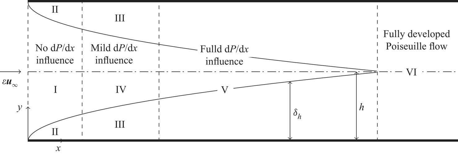
As shown in figure 1, the flow domain is divided into six asymptotic regions. Regions I and II pertain to the part of the channel where both the base flow and the perturbation flow are influenced by the confinement of the channel but the effect of the base-flow streamwise pressure gradient is negligible because of the small downstream distance. Regions III and IV are fully affected by the channel confinement, but the effect of the streamwise pressure gradient is mild in region IV and negligible in region III. In region V, the effects of confinement and pressure gradient are influential, but the base flow has not reached the fully developed Poiseuille profile. In region VI, the base flow is fully developed.
Asymptotic regions of the channel flow (not to scale). The boundary-layer thickness  $\delta _h$ is defined in the supplementary material § S2.

Region I is located at a  $x=O(1)$ distance from the inlet and extends along the whole wall-normal direction. The base and the perturbation flows are both inviscid there and the flow field can be adequately described by rapid distortion theory (Hunt Reference Hunt1973; Goldstein Reference Goldstein1978). The solution is expressed in terms of a velocity potential and the presence of the lower and upper plates is taken into account through the specification of appropriate boundary conditions obtained by asymptotic matching with the wall-normal velocity component of the boundary-layer disturbance. Region II is a viscous region underneath region I, where the boundary-layer thickness is much smaller than the spanwise wavelength, i.e.
 $\delta ^*/\lambda _z^* \ll 1$. This limit allows neglecting the spanwise viscous terms in the spanwise momentum equation because they are much smaller than the wall-normal viscous terms. The combined flow of regions I and II is studied in § 3.1.
Downstream of region II the boundary-layer thickness and the spanwise wavelength of the disturbance become of the same order, i.e.  $\lambda _z^*/\delta ^*=O(1)$, and thus the wall-normal and spanwise viscous terms are of comparable magnitude. This viscous region is named region III, where
 $\bar {x}=O(1)$ and the flow is governed by the linear unsteady boundary-region (LUBR) equations, that is the rigorous asymptotic limit of the Navier–Stokes equations for long-wavelength/low-frequency disturbances (Leib et al. Reference Leib, Wundrow and Goldstein1999). We assume that the base flow in regions II and III is of the Blasius type, hence the base-flow pressure gradient effect is negligible. Regions II and III occur in both boundary layers developing on the two channel walls. Region IV is the asymptotic region between the two regions III. Here, the base flow is inviscid, while the perturbation flow is viscous and influenced by the increased boundary-layer thickness and by the confinement of the channel flow. The pressure gradient only has a second-order effect. The combined flow of regions III and IV is discussed briefly in § 3.2.
The region of main interest is region V, where the flow is fully influenced by the channel confinement and the base-flow streamwise pressure gradient. It extends from the lower to the upper wall of regions III and IV. In region V, differently from region III where the Blasius solution applies, the base flow is not self-similar because of the unknown base-flow pressure gradient and non-parallel as the base-flow wall-normal velocity plays a key role. The latter vanishes further downstream in the fully developed region VI, where the parabolic Poiseuille profile occurs.
2.2. Governing equations and boundary conditions
The flow field is governed by the non-dimensional incompressible continuity and Navier–Stokes equations,
 $$\begin{gather} \boldsymbol{\nabla} \boldsymbol{\cdot} \boldsymbol{u} =0, \end{gather}$$
 $$\begin{gather}\frac{\partial \boldsymbol{u}}{\partial t}+(\boldsymbol{u}\boldsymbol{\cdot} \boldsymbol{\nabla} )\boldsymbol{u} ={-}\boldsymbol{\nabla} p+\frac{1}{R_\lambda}\nabla^2 \boldsymbol{u}. \end{gather}$$
The velocity  $\boldsymbol {u}$ and the pressure
 $p$ are expressed as the superposition of the base-flow velocity
 $\bar {\boldsymbol {U}}(\bar {x},y)$ and pressure
 $\bar {P}(\bar {x})=O(1)$ and the perturbation flow
 $\{\boldsymbol {u}',p'\}=\{u',v',w',p'\}$ as follows:
 \begin{equation} \{\boldsymbol{u},p\}=\underbrace{\begin{pmatrix}U(\bar{x},y)\\ k_xV(\bar{x},y)\\ 0 \\ P(\bar{x})\end{pmatrix}}_{{\bar{\boldsymbol{U}}, \bar{P}}} + \varepsilon \underbrace{\begin{pmatrix} \bar{u}_0(\bar{x},y)\\ \bar{v}_0(\bar{x},y)\\ \bar{w}_0(\bar{x},y) \\ \bar{p}_0(\bar{x}, y) \end{pmatrix} \, {\rm e}^{{\rm i}(k_z z - k_x t)}}_{{\boldsymbol{u}', p'}} + \mbox{c.c.},\end{equation}
and
 $$\begin{gather} \{ \bar{u}_0, \bar{v}_0\} =\{ \bar{u}^{(0)}, k_x \bar{v}^{(0)}\} + \left\{\frac{i k_z}{k_x}\bar{u}, i k_z \bar{v}\right\}, \end{gather}$$
 $$\begin{gather}\bar{w}_0 ={-} \frac{i k_x}{k_z}\bar{w}^{(0)} + \bar{w}, \end{gather}$$
 $$\begin{gather}\bar{p}_0 = \frac{k_x}{R_\lambda} \bar{p}^{(0)} + \frac{i k_z}{R_\lambda} \bar{p}. \end{gather}$$
Note that the main difference between  $\bar {v}$ and
 $\bar {v}^{(0)}$ and the corresponding components in (4.1) on page 176 of LWG99 is the missing factor
 $(2 \bar {x})^{1/2}$ in (2.8), which arises in LWG99's case because of the Blasius-similarity scaling. Substituting (2.8) into equations (2.6) and (2.7) and collecting the terms of
 $O(1)$ yields the base-flow boundary-layer equations,
 $$\begin{gather} \frac{\partial U}{\partial \bar{x}}+\frac{\partial V}{\partial y}=0, \end{gather}$$
 $$\begin{gather}U\frac{\partial U}{\partial \bar{x}}+V\frac{\partial U}{\partial y} ={-}\frac{\text{d} P}{\text{d} \bar{x}}+\frac{1}{\mathcal{F}} \frac{\partial^2 U}{\partial y^2}, \end{gather}$$
 $$\begin{gather}\frac{\partial P}{\partial y}=0, \end{gather}$$
for  $k_x, R_\lambda ^{-1} \ll 1$ and
 $\mathcal {F}=k_x R_\lambda = O(1)$. The pressure
 $P$ must be solved for, unlike simpler free-stream boundary-layer cases where the imposed pressure gradient is known. By exploiting the symmetry over the two channel halves, equations (2.10) and (2.11) are solved in the bottom half of the channel together with the integral form of the continuity equation,
 \begin{equation} \frac{1}{h} \int_0^hU\, \text{d}y=1, \end{equation}
and are subject to the no-slip and no-penetration conditions at the wall,
 \begin{equation} U=V=0 \text{ at } y=0, \end{equation}
and to the symmetry conditions at the centreline
 \begin{equation} \frac{\partial U}{\partial y}=V=0 \textrm{ at } y=h. \end{equation}
It must be noted that, although the boundary-layer approximation is adopted in the limit  $R_\lambda ^{-1} \rightarrow 0$, i.e. the streamwise viscous diffusion and the wall-normal pressure gradient are negligible, the flow is solved along the whole channel height. Other boundary-layer approximations, such as Schlichting (Reference Schlichting1934) and Collins & Schowalter (Reference Collins and Schowalter1962), instead split the channel domain in the near-wall regions and in the inner core.
A standard manipulation of the Navier–Stokes and continuity equations is carried out to obtain the equations of the perturbation flow. Because the perturbation pressure  $p'$ at the wall is unknown, it is common practice to eliminate the pressure from (2.6) and (2.7) by reducing them to a fourth-degree equation for the wall-normal velocity and a second-degree equation for the wall-normal vorticity (Kim, Moin & Moser Reference Kim, Moin and Moser1987; Schmid & Henningson Reference Schmid and Henningson2001). Using the compact notation of Kim et al. (Reference Kim, Moin and Moser1987), these equations read
 $$\begin{gather} \frac{\partial }{\partial t}\nabla^2 v = h_v+\frac{1}{R_\lambda}\nabla^4 v, \end{gather}$$
 $$\begin{gather}\frac{\partial \omega_y}{\partial t} = h_{\omega_y}+\frac{1}{R_\lambda}\nabla^2 \omega_y, \end{gather}$$
where
 \begin{equation} h_v={-}\frac{\partial }{\partial y}\left(\frac{\partial H_x}{\partial x}+\frac{\partial H_z}{\partial z} \right)+\left( \frac{\partial^2 }{\partial x^2} + \frac{\partial^2}{\partial z^2} \right) H_y, \quad h_{\omega_y}=\frac{\partial H_x}{\partial z}-\frac{\partial H_z}{\partial x}, \end{equation}
and
 \begin{equation} H_j ={-}\left(u \frac{\partial u_j}{\partial x} + v \frac{\partial u_j}{\partial y} + w\frac{\partial u_j}{\partial z} \right), \end{equation}
where the subscript  $j=x,y,z$ indicates the velocity component along the denoted coordinate. The wall-normal vorticity perturbation is
 \begin{equation} \omega_y' = \left[\frac{(i k_z)^2}{k_x}\bar{u}-k_x \frac{\partial \bar{w}}{\partial \bar{x}} \right]\, \textrm{e}^{\textrm{i}(k_z z -k_x t)} + \text{c.c.} ={-}\frac{k_z^2}{k_x} \bar{u} \, \textrm{e}^{\textrm{i}(k_z z -k_x t)} + O(k_x) + \text{c.c.}. \end{equation}
As the perturbation is elongated in the streamwise direction, vorticity is mostly created by the streamwise velocity perturbation  $\bar {u}$ and the contribution of the spanwise velocity
 $\bar {w}$ can be neglected. The equations of motion for the perturbation flow are derived by substituting (2.8) and (2.9) into (2.16) and (2.17), using (2.20) and collecting terms of
 $O(\varepsilon )$ for
 $k_x, R_\lambda ^{-1} \ll 1$ and
 $\mathcal {F} = O(1)$. They read
 \begin{align} &\left(i k_z^2 -\frac{k_z^4}{\mathcal{F}}- k_z^2 \frac{\partial V}{\partial y}+\frac{\partial^3 V}{\partial y^3}\right)\bar{v}- \left(k_z^2 V - \frac{\partial^2 V}{\partial y^2} \right) \frac{\partial \bar{v}}{\partial y} +\left({-}i + \frac{2 k_z^2}{\mathcal{F}} + \frac{\partial V}{\partial y} \right)\frac{\partial^2 \bar{v}}{\partial y^2}\nonumber\\ &\quad +V \frac{\partial^3 \bar{v}}{\partial y^3} +U\frac{\partial^3 \bar{v}}{\partial \bar{x}\partial y^2} -\frac{1}{\mathcal{F}}\frac{\partial^4 \bar{v}}{\partial y^4} -\left(k_z^2 U + \frac{\partial^2 U}{\partial y^2} \right)\frac{\partial \bar{v}}{\partial \bar{x}} -\left(k_z^2 \frac{\partial V}{\partial \bar{x}}-\frac{\partial^3 V}{\partial \bar{x}\partial y^2}\right)\bar{u}\nonumber\\ &\quad -2\frac{\partial^2 U}{\partial \bar{x}\partial y}\frac{\partial \bar{u}}{\partial \bar{x}} -2 \frac{\partial U}{\partial \bar{x}}\frac{\partial^2 \bar{u}}{\partial \bar{x}\partial y}-\frac{\partial V}{\partial \bar{x}}\frac{\partial^2 \bar{u}}{\partial y^2}=0, \end{align}
 \begin{align} &\left({-}i +\frac{k_z^2}{\mathcal{F}} +\frac{\partial U}{\partial \bar{x}} \right)\bar{u} +V \frac{\partial \bar{u}}{\partial y} +U \frac{\partial \bar{u}}{\partial \bar{x}} -\frac{1}{\mathcal{F}}\frac{\partial^2 \bar{u}}{\partial y^2} +\frac{\partial U}{\partial y}\bar{v}=0. \end{align}
Equations (2.21) and (2.22) are also satisfied by  $\{\bar {u}^{(0)},\bar {v}^{(0)}\}$. Equation (2.22) is the LUBR
 $x$-momentum equation as a consequence of (2.20). It is immediately clear from (2.21) and (2.22) that the most significant difference between the perturbation dynamics in the entrance region and in the fully developed Poiseuille-flow region further downstream lies in the presence of
 $\bar {u}$ and
 $\bar {v}$ in both equations in the entry-flow case, thus producing two-way coupling. When the flow is instead fully developed,
 $\partial U/\partial \bar {x}$ and
 $V$ are null and therefore, like in the Orr–Sommerfeld equation describing the classical linear stability, (2.21) can be solved by itself to find the wall-normal velocity, which then drives the streamwise disturbance through the lift-up term
 $\bar {v} \partial U/\partial y$ in the vorticity equation (Schmid & Henningson Reference Schmid and Henningson2001).
Equations (2.21) and (2.22) are solved numerically subject to
 \begin{equation} \bar{u}=\bar{v}=\frac{\partial \bar{v}}{\partial y}=0, \end{equation}
at  $y=0$ and
 $y=2h$. The spanwise velocity component
 $\bar {w}$ is computed a posteriori from the continuity equation,
 \begin{equation} \bar{w}={-} \left( \frac{\partial \bar{u}}{\partial \bar{x}}+\frac{\partial \bar{v}}{\partial y} \right). \end{equation}
The pressure is computed a posteriori by substituting (2.8) into the spanwise momentum equation and collecting terms of  $O(\varepsilon )$,
 \begin{equation} \bar{p}= \frac{\mathcal{F}}{k_z^2} \left[ \left({-}i + \frac{k_z^2}{\mathcal{F}} \right)\bar{w} + U \frac{\partial \bar{w}}{\partial \bar{x}} + V \frac{\partial \bar{w}}{\partial y} -\frac{1}{\mathcal{F}} \frac{\partial^2 \bar{w}}{\partial y^2} \right]. \end{equation}
The base-flow equations (2.10) and (2.11) and the LUBR equations (2.21) and (2.22) are parabolic and thus solved through a downstream marching procedure. The specification of the appropriate initial conditions is of crucial importance. We have thus devoted great attention to the formulation of physically meaningful initial conditions for both the base and the perturbation flows. The initial base-flow velocity profile has usually been assumed uniform (Bodoia & Osterle Reference Bodoia and Osterle1962; Van Dyke Reference Van Dyke1969; Wilson Reference Wilson1970). We instead take into account the interaction between the oncoming flow and the channel walls by deriving an asymptotic solution composed of the Blasius flow near the walls (inner solution) and the inviscid flow in the channel core that is distorted by the developing boundary layers (outer solution). A similar approach was employed by Rubin, Khosla & Saari (Reference Rubin, Khosla and Saari1977). The small- $x$ base-flow asymptotic initial condition used to solve the base-flow equations (2.10) and (2.11) is described in § S1.1.
Perturbation-flow inflow conditions for open boundary-layer computations are often specified as the continuous spectrum of the Orr–Sommerfeld/Squire equations (Jacobs & Durbin Reference Jacobs and Durbin2001; Brandt, Schlatter & Henningson Reference Brandt, Schlatter and Henningson2004) or by selecting optimal perturbations, as those obtained for the flat plate case by Andersson et al. (Reference Andersson, Berggren and Henningson1999) and Luchini (Reference Luchini2000). As inflow conditions, Buffat et al. (Reference Buffat, Le Penven, Cadiou and Montagnier2014) imposed optimal disturbances within one of the boundary layers near the channel entrance, while perturbations were absent in the inviscid core. However, as also discussed in the Introduction (refer also to Ricco et al. (Reference Ricco, Walsh, Brighenti and McEligot2016)), neither the continuous spectrum of the Orr–Sommerfeld/Squire equations nor the optimal perturbations have to date been proven to be physically realizable perturbations that can be used as inflow conditions.
We instead prescribe initial conditions that are superposed on the inviscid core flow and are fully consistent with the oncoming vortical disturbances at  $\bar {x}=0$, given in (2.1). Like the base flow, these initial conditions are expressed as asymptotic composite solutions of a viscous inner solution within the boundary layer and an outer solution where the base flow is inviscid in the channel core. We do not use optimal perturbations as they are the output of an optimization procedure where the streamwise and spanwise velocities vanish in the inviscid core flow outside of the boundary layer, while we are interested in their entrainment of vortical disturbances that occupy the entire cross-plane at the channel mouth. The initial condition is not imposed at
 $\bar {x}=0$ because the wall-normal base-flow velocity is singular there and because the flow field is governed by the full Navier–Stokes equations in the immediate surroundings of the channel mouth. Therefore, the initial conditions are imposed at a location
 $0<\bar {x}_0 \ll 1$.
Section 3.1 presents results for the development of the perturbation flow at small- $x$ locations where the base-flow pressure gradient is negligible. These flow fields are small-
 $x$ asymptotic solutions of the flow in region V and can therefore be used as initial conditions to solve (2.21) and (2.22) along the channel, where the base-flow streamwise pressure gradient is fully influential.
2.3. Critical streamwise location for linear stability
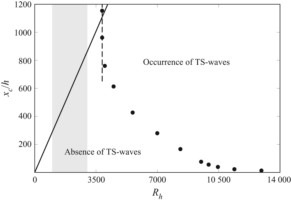
As we focus on the transient growth of vortical disturbances in the entrance region, a first step is to report, as a function of the Reynolds number, the streamwise distance upstream of which TS-waves do not appear. Garg & Gupta (Reference Garg and Gupta1981a) extended their classical spatial stability study in Gupta & Garg (Reference Gupta and Garg1981a) and Garg & Gupta (Reference Garg and Gupta1981b) to include the non-parallel base-flow effects. The main result is that the entrance flow is always more linearly stable than the fully developed flow at the same bulk Reynolds number. Figure 2 shows Reference Garg and GuptaGarg & Gupta's (Reference Garg and Gupta1981a) computed neutral stability location  $x_c/h$ as a function of the Reynolds number
 $R_h=h R_\lambda =U_\infty ^* h^*/\nu ^*$ (black circles). The channel flow is stable according to classical stability theory (absence of TS-waves) to the left of the black circles. For
 $R_h<3848$, which corresponds to the classical stability Reynolds number
 ${R_p=U_p^* h^*/\nu ^*=3R_h/2=5772}$, where
 $U_p^*$ is the maximum velocity of the parabolic Poiseuille profile, the flow is stable at any streamwise location. At
 $R_h=3848$ the flow is linearly unstable downstream of
 $x_c/h \approx 1000$, that is, where it has reached the Poiseuille profile. As
 $R_h$ increases further, the entrance flow becomes unstable at decreasing streamwise locations. The solid line denotes the end of the entry laminar flow region according to our adopted definition based on the second derivative of the base-flow velocity at the centreline (refer to the supplementary material § S2).
Black circles: streamwise location downstream of which the channel-entrance flow becomes unstable according to classical stability theory, i.e. TS-waves start to grow. The data points have been rescaled from the original ones by Garg & Gupta (Reference Garg and Gupta1981a). The dashed line denotes the critical Reynolds number  $R_h=3848$ for the fully developed Poiseuille flow. Solid black line: end location of the entry laminar channel flow region, according to our definition based on the second derivative of the base-flow velocity at the centreline, as discussed in the supplementary material § S2. The grey area illustrates the range of Reynolds numbers for the flows studied in our work.

We focus on Reynolds numbers in the range  $1000< R_h<3500$ (marked by the light grey area in figure 2), i.e. small enough for TS-waves not to appear and large enough for algebraically growing perturbations or transition to turbulence to have been observed in experimental studies. Reference Patel and HeadPatel & Head's (Reference Patel and Head1969) air channel experiments, which are particularly relevant because the entrance flow was defined as ‘sufficiently disturbed’, show that intermittency is absent for
 $R_h<675$ and the flow is turbulent for
 $R_h>1250$. Kao & Park (Reference Kao and Park1970) report that no instabilities were detected for
 $R_h<1250$ in a water channel and Nishioka et al. (Reference Nishioka, Iida and Ichikawa1975) measured subcritical instabilities triggered by a vibrating ribbon at their lowest
 $R_h=2000$. Carlson et al. (Reference Carlson, Widnall and Peeters1982) later found transition in a channel at
 $R_h=1000$ and Nishioka & Asai (Reference Nishioka and Asai1985) concluded that no sustained turbulence exists for
 $R_h<667$ by observing the decay of large disturbances from the channel inlet.
2.4. Numerical procedures
The base-flow continuity and boundary-layer equations (2.10) and (2.11), supplemented by the integral form of the continuity equation (2.13), are discretized according to a scheme that is an improved version of that used by Bodoia & Osterle (Reference Bodoia and Osterle1962), whereby (2.13) is integrated using the trapezoidal rule. The base-flow streamwise velocity and pressure fields are computed simultaneously and the base-flow wall-normal velocity is computed a posteriori through the continuity equation. A difference from Bodoia & Osterle (Reference Bodoia and Osterle1962) regards the treatment of the nonlinear convective terms in the base-flow  $x$-momentum equation (2.11). In their paper, these terms are linearized, i.e. the values at the previous
 $x$ locations are used in the nonlinear terms. Here, we instead use a predictor–corrector method for the computation of the convective terms at step
 $n$. In the predictor step
 $n-1$, an initial approximation of the streamwise velocity and pressure fields is calculated via the linearized discrete equations as in Bodoia & Osterle (Reference Bodoia and Osterle1962). In the corrector step, new values of
 $U^n$ and
 $P^n$ are computed, using
 $U^{n-1}$ and
 $P^{n-1}$ in the discretization of the convective terms instead of those at the previous streamwise location. This procedure is repeated iteratively until convergence is reached. The convergence criterion is based on the wall-normal velocity gradient at the wall,
 $\partial U/\partial y|_{y=0}$. The asymptotic composite solution of the base flow derived in the the supplementary material § S1 is used as initial condition at small
 $\bar {x}$ values.
The LUBR (2.21) and (2.22) are discretized using backward and central finite-difference schemes in  $\bar {x}$ and
 $y$, respectively. The degree of the wall-normal velocity equation (2.21) is reduced from fourth to second by defining the wall-normal second derivative of
 $\bar {v}$ as a new variable. The resulting system is written in the form of a block tridiagonal matrix and solved at each
 $\bar {x}$ by the Thomas algorithm (Cebeci Reference Cebeci2002). The asymptotic composite solution given in § 3.1 is used as initial condition at small
 $\bar {x}$ values.
3. Flow development in regions I, II, III and IV
In this section we discuss the theoretical and numerical results of the base and perturbation flows near the channel entrance, where the effect of the channel confinement plays a leading role, but the influence of the base-flow pressure gradient is negligible at leading order. This mathematical analysis is important because, through the asymptotic formulation, the physical flow features near the entrance are revealed and the flow evolution further downstream inside the channel can be computed. As explained at the end of § 2, the results obtained in this section will indeed specify the appropriate initial conditions for the computation of the base and the perturbation flows in region V, where the dynamics is fully influenced by the streamwise pressure gradient. The development of the base flow in regions I and II is presented in the supplementary material § S1.
The precise specification of the flow at the channel entrance is relevant as our interest lies in the mathematical description of the inlet profiles to start the computations and to understand how the vortical disturbances are entrained in the channel mouth and how they evolve in the entrance region. The initial development of the perturbation flow, i.e. where the flow is fully influenced by the channel confinement and only mildly by the base-flow streamwise pressure, is studied via matched asymptotic expansions. Asymptotic composite solutions are derived for regions I and II in § 3.1 and for regions III and IV in § 3.2.
3.1. Perturbation flow in regions I and II
All the composite solutions in this section pertain to the lower channel half and symmetries are used to find the quantities in the upper channel half.
In region I the base flow is uniform and inviscid, the perturbation flow is inviscid and  $\bar {x}\ll 1$ with
 $\mathcal {F}=k_x R_\lambda =O(1)$. The flow field can thus be adequately described by rapid distortion theory (Goldstein Reference Goldstein1978). The velocity is expressed as
 \begin{align} \boldsymbol{u}_{out} &=\hat{\boldsymbol{i}} + \varepsilon [\boldsymbol{u}^{(1)}(\bar{x},y) + k_x \boldsymbol{u}^{(1)}_1(\bar{x},y)] \, \textrm{e}^{\textrm{i}(k_z z-k_x t])} + \text{c.c.} \nonumber\\ &=\hat{\boldsymbol{i}} + \varepsilon ( \boldsymbol{u}_\infty + \boldsymbol{\nabla} \phi + k_x \boldsymbol{\nabla} \phi_1) + \text{c.c.}. \end{align}
The velocity  $\boldsymbol {u}^{(1)}$ is due to the interaction of the free-stream gust (2.1) with the channel walls, while
 $\boldsymbol {u}^{(1)}_1$ is generated by the wall-normal boundary-layer perturbation velocity via the gradient
 $\boldsymbol {\nabla } \phi _1$. The perturbation potential
 $\phi$ satisfies Laplace's equation
 \begin{equation} \nabla^2{\phi}=0, \end{equation}
subject to
 \begin{equation} \frac{\partial \phi}{\partial y}+u_{\infty y} = 0 \text{ at } y=0,2h, \quad x>0,\end{equation}
where  $u_{\infty y}(y=0,2h)=( \hat {u}_{y+}^\infty +\hat {u}_{y-}^\infty )\exp [i (k_x x + k_z z - k_x t)]$ is the gust wall-normal velocity found from (2.1) as the channel walls are approached. Expressions (3.3a) are the no-penetration boundary conditions at the walls for the wall-normal velocity. To solve (3.2) in the infinite strip
 $-\infty < x < \infty , 0 \leq y \leq 2h$, one needs boundary conditions at
 $y = 0,2h$ for
 $x < 0$, which are unknown. However, the interest is in the solution for
 $x \gg 1$, found by separation of variables,
 \begin{equation} \phi=\frac{\hat{u}_{y+}^\infty+\hat{u}_{y-}^\infty}{\gamma (\textrm{e}^{2 \gamma h}- \textrm{e}^{{-}2 \gamma h} )}[(\textrm{e}^{{-}2 \gamma h}-1 )\, \textrm{e}^{\gamma y}+(\textrm{e}^{2 \gamma h}-1 ) \, \textrm{e}^{-\gamma y}]\, \textrm{e}^{\textrm{i}[k_x(x-t)+k_z z]}, \end{equation}
where  $\gamma =\sqrt {k_x^2+k_z^2}$. The velocity components of
 $\boldsymbol {u}^{(1)}=\{u_x^{(1)},u_y^{(1)},u_z^{(1)}\}$ in (3.1) are
 \begin{align} u_m^{(1)}(\bar{x},y)&= \frac{i k_m \, \textrm{e}^{\textrm{i}\bar{x}}(\hat{u}_{y+}^\infty+\hat{u}_{y-}^\infty)}{\gamma (\textrm{e}^{2 \gamma h}- \textrm{e}^{{-}2 \gamma h} )}[(\textrm{e}^{{-}2 \gamma h}-1 )\, \textrm{e}^{\gamma y}+(\textrm{e}^{2 \gamma h}-1 ) \, \textrm{e}^{-\gamma y}] \nonumber\\ &\quad +\hat{u}_{m+}^\infty \, \textrm{e}^{\textrm{i}\bar{x}+i k_y y} +\hat{u}_{m-}^\infty \, \textrm{e}^{\textrm{i}\bar{x}-i k_y y}, \end{align}
for  $m=x,z$ and
 \begin{align} u_y^{(1)}(\bar{x},y) &= \frac{(\hat{u}_{y+}^\infty+\hat{u}_{y-}^\infty) \, \textrm{e}^{\textrm{i}\bar{x}}}{ \textrm{e}^{2 \gamma h}- \textrm{e}^{- 2\gamma h}} [(\textrm{e}^{{-}2 \gamma h}-1)\, \textrm{e}^{\gamma y} + (1- \textrm{e}^{2 \gamma h}) \, \textrm{e}^{-\gamma y}] \nonumber\\ &\quad +\hat{u}_{y+}^\infty \, \textrm{e}^{\textrm{i}\bar{x}+i k_y y} +\hat{u}_{y-}^\infty \, \textrm{e}^{\textrm{i}\bar{x}-i k_y y}. \end{align}
Using (2.8) and (2.9), the leading-order streamwise and wall-normal velocities in region I are
 \begin{equation} \left.\begin{array}{c} \bar{u}_{out} = 0, \\ \bar{v}_{out} ={-}\dfrac{i \, \textrm{e}^{\textrm{i} \bar{x}}}{k_z} \left\{ \dfrac{\hat{u}_{y+}^\infty + \hat{u}_{y-}^\infty}{ \textrm{e}^{2 \gamma h}- \textrm{e}^{- 2\gamma h}} [ (\textrm{e}^{{-}2 \gamma h}-1)\, \textrm{e}^{ \gamma y} +(1- \textrm{e}^{2 \gamma h})\, \textrm{e}^{-\gamma y} ]\right.\\ \quad + \left.\hat{u}_{y+}^\infty \, \textrm{e}^{ \textrm{i} k_y y} + \hat{u}_{y-}^\infty \, \textrm{e}^{-\textrm{i} k_y y} \vphantom{\dfrac{\hat{u}_{y+}^\infty + \hat{u}_{y-}^\infty}{ \textrm{e}^{2 \gamma h}- \textrm{e}^{- 2\gamma h}}}\right\}. \end{array}\right\} \end{equation}
Similar solutions have been found by Duck (Reference Duck2005) in his analysis of the channel-entrance flow, where the boundary-layer perturbation was given by the Luchini mode (Luchini Reference Luchini1996). The leading-order spanwise velocity  $\bar {w}_{out}$ can be found from (3.5) for
 $m=z$ or by using (3.7) and the continuity equation (2.24). It reads
 \begin{align}
\bar{w}_{out}&= \frac{i (\hat{u}_{y+}^\infty +
\hat{u}_{y-}^\infty)\, \textrm{e}^{\textrm{i} \bar{x}}}{{
\textrm{e}^{2 \gamma h}- \textrm{e}^{- 2\gamma h}}} [
(\textrm{e}^{{-}2 \gamma h}-1)\, \textrm{e}^{ \gamma y} +
(\textrm{e}^{ 2 \gamma h}-1)\, \textrm{e}^{-\gamma y} ]\notag\\
&\quad +
\hat{u}_{z+}^\infty \, \textrm{e}^{\textrm{i} \bar{x} + i
k_y y} + \hat{u}_{z-}^\infty \, \textrm{e}^{\textrm{i}
\bar{x} - i k_y y}.
\end{align}
As the channel walls are approached,  $\bar {w}_{out}$ drives the inner flows in the viscous regions II. In region II the spanwise viscous diffusion effects do not play a leading role and thus the flow field is described by the unsteady boundary-layer equations (LWG99). The inner solution for the spanwise velocity is
 $\bar {w}_{in}=\bar {w}_{com} F'(\eta )$, found by use of (4.13) in LWG99, where the common parts
 $\bar {w}_{com}$ are
 \begin{equation} \bar{w}_{com}(\bar{x}) =\bar{w}_{out}(y=0,2h) =\frac{\pm i (\hat{u}_{y+}^\infty + \hat{u}_{y-}^\infty)\, \textrm{e}^{\textrm{i} \bar{x}}}{{ \textrm{e}^{2 \gamma h}- \textrm{e}^{- 2\gamma h}}} ( \textrm{e}^{{-}2 \gamma h}+\, \textrm{e}^{2 \gamma h}-2 )+ \textrm{e}^{\textrm{i} \bar{x}} (\hat{u}_{z+}^\infty + \hat{u}_{z-}^\infty), \end{equation}
where the  $+$ sign is used for
 $y=0$ and the
 $-$ sign is used for
 $y=2h$.
The composite spanwise velocity in the lower channel half is
 \begin{align} \bar{w} &=\frac{i (\hat{u}_{y+}^\infty + \hat{u}_{y-}^\infty)\, \textrm{e}^{\textrm{i} \bar{x}}}{{ \textrm{e}^{2 \gamma h}- \textrm{e}^{- 2\gamma h}}} [(\textrm{e}^{{-}2 \gamma h}-1)\, \textrm{e}^{ \gamma y} +(\textrm{e}^{ 2 \gamma h}-1)\, \textrm{e}^{-\gamma y} ]\nonumber\\ &\quad + \hat{u}_{z+}^\infty \, \textrm{e}^{\textrm{i} \bar{x} + i k_y y} + \hat{u}_{z-}^\infty \, \textrm{e}^{\textrm{i} \bar{x} - i k_y y} + \bar{w}_{com} (F' - 1). \end{align}
The solution (3.10) is not needed for the numerical computation in region V because  $\bar {w}$ is absent from equations (2.21) and (2.22). However, it is crucial to compute
 $\bar {w}_{com}$ because it univocally determines the amplitude of the inner streamwise and wall-normal velocities. The streamwise velocity component in region I of the lower channel half is therefore
 $\bar {u}_{in}=\bar {w}_{com}\bar {x} \eta F''/2$, found using (4.13) in LWG99. As
 $\bar {u}_{out}=0$,
 \begin{equation} \bar{u}=\bar{w}_{com}\bar{x} \frac{\eta F''}{2}, \end{equation}
is valid across the whole lower channel half. The asymptotic approach is clearly an invaluable tool as the amplitude of the streamwise perturbation velocity is uniquely linked to the oncoming free-stream flow characteristics through  $\bar {w}_{com}$, given in (3.9). In other approaches, based on eigenvalue solutions or optimal perturbations, this essential relation is absent and therefore the streak amplitude must be assigned arbitrarily.
The composite wall-normal velocity  $\bar {v}$ is found by first summing the outer solution (3.7) and the inner solution obtained by multiplying the region-II wall-normal velocity (4.13) in LWG99 by the amplitude
 $\bar {w}_{com}$ and by
 $(2 \bar {x})^{1/2}$ on using (4.1) in LWG99. The common part, i.e. the large-
 $\eta$ limit of the region-II solution, is then subtracted. The common part also emerges from the second-order term of the small-
 $y$ Taylor expansion of the outer solution (3.7), while the leading-order term vanishes because of the no-penetration condition (3.3a). The composite wall-normal velocity is therefore
 \begin{align} \bar{v} &= \underbrace{ -\frac{i \, \textrm{e}^{\textrm{i} \bar{x}}}{k_z} \left\{ \frac{\hat{u}_{y+}^\infty + \hat{u}_{y-}^\infty}{ \textrm{e}^{2 \gamma h}- \textrm{e}^{- 2\gamma h}} [(\textrm{e}^{{-}2 \gamma h}-1)\, \textrm{e}^{ \gamma y} + (1- \textrm{e}^{2 \gamma h})\, \textrm{e}^{-\gamma y} ] + \hat{u}_{y+}^\infty \, \textrm{e}^{ \textrm{i} k_y y} + \hat{u}_{y-}^\infty \, \textrm{e}^{-\textrm{i} k_y y} \right\} }_{\scriptsize \mbox{outer} \ \mbox{solution}}\nonumber\\ &\quad +\underbrace{ \frac{\bar{w}_{com}}{4} \left( \frac{2 \bar{x}}{\mathcal{F}} \right)^{1/2} ( \eta^2 F'' - 3 \eta F' - F ) }_{\scriptsize \mbox{inner} \ \mbox{solution}}+ \underbrace{ \bar{w}_{com} \left( \frac{2 \bar{x}}{\mathcal{F}} \right)^{1/2} \eta }_{\scriptsize \mbox{common} \ \mbox{part}}. \end{align}
The initial conditions for  $\{ \bar {u}^{(0)}, \bar {v}^{(0)}, \bar {w}^{(0)}\}$, defined in (2.9), are also found through a composite solution. The solution for the streamwise velocity
 $\bar {u}^{(0)}$ is found by combining the outer solution (3.5) for
 $m=x$ and the inner solution given by (4.13) in LWG99, valid for
 $\mathcal {F} = O(1)$ and
 $\bar {x}\ll 1$. It reads
 \begin{equation} \bar{u}^{(0)} = \textrm{e}^{\textrm{i} \bar{x}} (\hat{u}_{x+}^\infty \, \textrm{e}^{\textrm{i} k_y y} + \hat{u}_{x-}^\infty \, \textrm{e}^{-\textrm{i} k_y y})+ (\hat{u}_{x+}^\infty + \hat{u}_{x-}^\infty) \, \textrm{e}^{\textrm{i} \bar{x}} \left[\frac{(\eta F')'+F'}{2} - 1\right]. \end{equation}
The first term in (3.5) can be neglected because it is  $O(k_x)$. The inner solution for the wall-normal velocity
 $\bar {v}^{(0)}$ is found by (4.13) in LWG99, which is also valid for
 $\mathcal {F} = O(1)$ and
 $\bar {x}\ll 1$. It reads
 \begin{equation} \bar{v}^{(0)}_{in} =\frac{\hat{u}_{x+}^\infty + \hat{u}_{x-}^\infty}{2 (2 \bar{x}\mathcal{F})^{1/2}} [\eta (\eta F')' - F]. \end{equation}
Physically, this perturbation velocity represents a wall-normal blowing/suction effect, an unsteady analogue to the one experienced by the base-flow Blasius boundary layer. In the Blasius case, the base wall-normal velocity is generated by the free-stream uniform  $U^*_\infty$, while
 $\bar {v}^{(0)}_{out}$ is driven by
 $\bar {u}^{(0)}_{out}$. As
 $\bar {u}^{(0)}_{out}(y=0,2h)=\hat {u}_{x+}^\infty + \hat {u}_{x-}^\infty$, the physical transpiration wall-normal velocities from the two boundary layers attached to the channel walls are opposite and equal in magnitude at each time and
 $z$. They induce the inviscid velocity field
 $\boldsymbol {u}^{(1)}_1$ in (3.1) and the associated wall-normal pressure gradient that, differently from
 $\bar {v}$ which may be finite at the centreline, takes
 $\bar {v}^{(0)}_{out}$ to zero at
 $y=h$. The velocity potential
 $\phi _1$ satisfies
 \begin{equation} \nabla^2{\phi_1}=0, \end{equation}
subject to
 $$\begin{gather} \frac{\partial \phi_1}{\partial y} = \lim_{\eta \rightarrow \infty} \bar{v}^{(0)}_{in} = \beta \frac{\hat{u}_{x+}^\infty + \hat{u}_{x-}^\infty}{2 (2 \bar{x}\mathcal{F})^{1/2}} \, \textrm{e}^{\textrm{i} k_z z-i k_x t} \text{ at } y=0, \quad x>0, \end{gather}$$
 $$\begin{gather}\frac{\partial \phi_1}{\partial y} ={-} \beta \frac{\hat{u}_{x+}^\infty + \hat{u}_{x-}^\infty}{2 (2 \bar{x}\mathcal{F})^{1/2}} \, \textrm{e}^{\textrm{i} k_z z-i k_x t} \text{ at } y=2h, \quad x>0. \end{gather}$$
Similar to the problem of solving (3.2), (3.15) cannot be solved in the infinite strip  $-\infty < x < \infty$, 0
 $\leq y \leq 2h$ because the boundary conditions at
 $y = 0,2h$ for
 $x < 0$ are unknown. In our region of interest,
 $x \gg 1$, the second derivative of
 $\phi _1$ with respect to
 $x$ is asymptotically smaller than the other derivatives as long as
 $k_x \ll \bar {x} \ll 1$ because of the
 $(2\bar {x})^{-1/2}$ behaviour of the boundary conditions (3.16a) and (3.16b). It follows that, by separating the variables and expressing
 $\phi _1=\hat \phi _1(y)\exp (i k_z z-i k_x t)/(2 \bar {x})^{1/2}$, we find
 \begin{equation} \hat \phi_1 =\beta \frac{\hat{u}_{x+}^\infty + \hat{u}_{x-}^\infty}{2 k_z \mathcal{F}^{1/2}} \left[ \frac{ \textrm{e}^{k_z(y-h)}+\, \textrm{e}^{{-}k_z(y-h)}}{ \textrm{e}^{{-}k_z h}- \textrm{e}^{k_zh}} \right]. \end{equation}
The composite  $\bar {v}^{(0)}$ in the lower channel half reads
 \begin{equation} \bar{v}^{(0)} = \frac{\hat{u}_{x+}^\infty + \hat{u}_{x-}^\infty}{2(2 \bar{x}\mathcal{F})^{1/2}} \left\{ \eta (\eta F')' - F +\beta \left[ \frac{ \textrm{e}^{k_z(y-h)}- \textrm{e}^{{-}k_z(y-h)}}{ \textrm{e}^{{-}k_z h}- \textrm{e}^{k_zh}}-1 \right] \right\}. \end{equation}
The symmetry is again used to construct the solution in the upper channel half. It is easily verified that  $k_x\bar {v}^{(0)}$ is asymptotically smaller than
 $i k_z \bar {v}$ and
 $\bar {u}^{(0)}$ in the region of interest
 $k_x/R_\lambda \ll \bar {x} \ll 1$, as required by expansion (2.9).
Differently from the leading-order components where  $\bar {w}_{out}$ is needed to determine the amplitude of
 $\{\bar {u}_{in},\bar {v}_{in}\}$, it is not necessary to compute
 $\bar {w}^{(0)}$ as we have already found
 $\{\bar {u}^{(0)},\bar {v}^{(0)}\}$ to start the integration of the boundary-region equations (2.21) and (2.21). The component
 $\bar {w}^{(0)}$ induces a boundary-layer perturbation of the same order as the streamwise slip velocity, and it would be needed if an initial condition of second-order accuracy were constructed. The spanwise velocity
 $\bar {w}^{(0)}$ can be computed by the composite solution, where the outer solution is obtained by using (3.17) and by solving (A3) and (A4) in Ricco (Reference Ricco2009) when
 $\mathcal {F}=O(1)$ (it is null when
 $\mathcal {F} \gg 1$). The pressure disturbance in (A3) in Ricco (Reference Ricco2009) is found by again using (3.17) and equation (3.2) in LWG99. We note that analytical expression for
 $\{\bar {u}_{in}^{(0)},\bar {v}_{in}^{(0)}\}$ are instead valid for
 $\mathcal {F}=O(1)$.
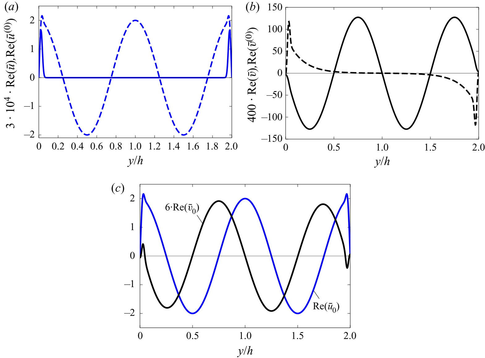
Figure 3 shows velocity profiles for a streamwise case, i.e.  $\hat u^\infty _{x+}=\hat u^\infty _{x-}$. The streamwise velocity profiles
 ${\rm Re}(\bar {u})$ and
 ${\rm Re}(\bar {u}^{(0)})$ are symmetric with respect to the centreline (a), while
 ${\rm Re}(\bar {v})$ is antisymmetric (b) because
 $\hat u^\infty _{y+}$ and
 $\hat u^\infty _{y-}$ have opposite signs due to the continuity relation (2.2). The wall-normal velocity
 ${\rm Re}(\bar {v}^{(0)})$ is antisymmetric because it is generated by the opposite boundary-layer transpiration velocities given in (3.16a) and (3.16b). Panel (c) of figure 3 shows that the combined
 ${\rm Re}(\bar {u}_0)$ is symmetric and the combined
 ${\rm Re}(\bar {v}_0)$ is antisymmetric. The composite solutions (3.11), (3.12), (3.13) and (3.18) for
 $\bar {u},\bar {v},\bar {u}^{(0)}$ and
 $\bar {v}^{(0)}$ in regions I and II are used as initial conditions for the computation in regions V and VI.
Real parts of composite symmetric velocity profiles in regions I and II for  $\bar {x}=10^{-4}, R_\lambda =1000, k_x=0.001, k_y=2{\rm \pi} , \hat u^\infty _{x+}=\hat u^\infty _{x-}=\hat u^\infty _{z+}=\hat u^\infty _{z-}=1, \hat u^\infty _{y+}=-2=-\hat u^\infty _{y-}$ and
 $h=1$. (a) Real parts of
 $\bar {u}$ (solid line) and
 $\bar {u}^{(0)}$ (dashed line). (b) Real parts of
 $\bar {v}$ (solid line) and
 $\bar {v}^{(0)}$ (dashed line). (c) Real parts of the velocity components
 $\bar {u}_0$ and
 $\bar {v}_0$.

3.2. Perturbation flow in regions III and IV
The outer expressions (3.7) do not take into account the viscous decay as they are valid in the very proximity of  $\bar {x}=0$. As the outer flow develops downstream through region IV, viscous effects become important. The flow in regions III and IV can be found by a composite solution. The expression for the outer velocity field in region IV is derived analytically by writing
 \begin{equation} \boldsymbol{u}=\left\{\frac{\partial \psi}{\partial y}, -\frac{\partial \psi}{\partial x} ,0 \right\} +\varepsilon \boldsymbol{u}_{out}\, \textrm{e}^{\textrm{i}(k_z z-k_x t)} + \text{c.c.}, \end{equation}
where the streamfunction  $\psi (\bar {x},y)$ is given in the supplementary material (S1.6) and (S1.11). The outer velocity
 $\boldsymbol {u}_{out}$ satisfies the parabolic region-IV momentum equations (5.9) on page 181 in LWG99, but in our case the initial conditions are given by our solution in region I, i.e. (3.7) for
 $\bar {u}_{out}$ and
 $\bar {v}_{out}$, and (3.8) for
 $\bar {w}_{out}$. The solution is found by separation of variables,
 \begin{equation} \left.\begin{array}{c} \bar{u}_{out} = 0, \\ \begin{aligned} \bar{v}_{out} & ={-}\dfrac{i}{k_z} \left\{ \dfrac{(\hat{u}_{y+}^\infty + \hat{u}_{y-}^\infty )\, \textrm{e}^{\textrm{i} \bar{x}} } { \textrm{e}^{2 \gamma h}- \textrm{e}^{- 2\gamma h}} [(\textrm{e}^{{-}2 \gamma h}-1)\, \textrm{e}^{ \gamma \psi} +(1- \textrm{e}^{2 \gamma h})\, \textrm{e}^{-\gamma \psi} ]\right.\\ & \quad \left. \vphantom{\dfrac{i}{k_z}} + \textrm{e}^{\textrm{i}\bar{x} - (k_y^2 + k_z^2)\bar{x}/\mathcal{F}} (\hat{u}_{y+}^\infty \, \textrm{e}^{ \textrm{i} k_y \psi} +\hat{u}_{y-}^\infty \, \textrm{e}^{-\textrm{i} k_y \psi})\right\}, \end{aligned}\\ \begin{aligned} \bar{w}_{out} & = \dfrac{i (\hat{u}_{y+}^\infty + \hat{u}_{y-}^\infty)\, \textrm{e}^{\textrm{i} \bar{x}}}{{ \textrm{e}^{2 \gamma h}- \textrm{e}^{- 2\gamma h}}} [(\textrm{e}^{{-}2 \gamma h}-1)\, \textrm{e}^{ \gamma \psi} +(\textrm{e}^{ 2 \gamma h}-1)\, \textrm{e}^{-\gamma \psi} ]\\ & \quad + \textrm{e}^{\textrm{i}\bar{x} - (k_y^2 + k_z^2)\bar{x}/\mathcal{F}} (\hat{u}_{z+}^\infty \, \textrm{e}^{\textrm{i} k_y \psi} + \hat{u}_{z-}^\infty \, \textrm{e}^{- i k_y \psi}). \end{aligned} \end{array}\right\} \end{equation}
As depicted in figure 1, the base-flow pressure gradient only has a second-order effect through the  $\bar {x}$-dependency of
 $\psi (\bar {x},y)$. The inner solution is found numerically by solving the boundary-region equations (5.2)–(5.5) on page 180 of LWG99, complemented by mixed-type boundary conditions obtained by asymptotically matching the solution of the large-
 $\eta$ (5.16)–(5.19) on page 181 of LWG99 with the outer solution (3.20). This numerical calculation is, however, not pursued herein because our region-V solution includes the solutions of regions III and IV and covers the whole streamwise flow evolution as the base-flow pressure gradient is accounted for at leading order.
4. Flow development in regions V and VI
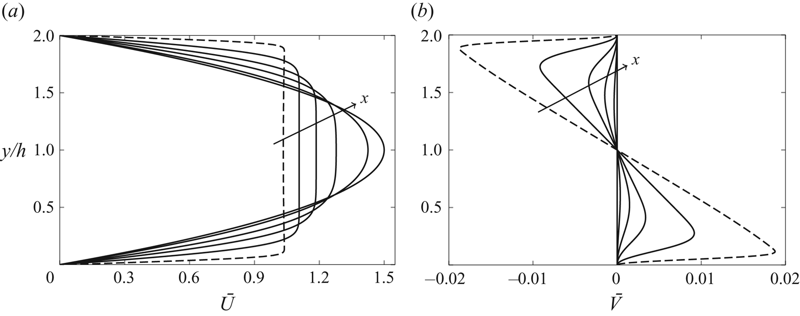
In § 3 the base and perturbation flows are influenced by the confinement of the channel, but the streamwise location is sufficiently upstream for the base-flow streamwise pressure gradient not to play a leading-order role. In the present section, we consider regions V and VI, i.e. downstream locations where the base-flow pressure gradient instead plays a leading-order role in the base flow and therefore in the perturbation flow. In region VI, the pressure gradient adjusts downstream to a constant value as the base flow develops to the fully developed Poiseuille flow. The base-flow profiles are obtained by solving (2.11)–(2.13) and the perturbation profiles are found by solving (2.21) and (2.22). The base-flow streamwise and wall-normal velocity profiles across the channel are shown in figure 4 for various streamwise positions. The base-flow streamwise velocity evolves to the parabolic Poiseuille profile, while the wall-normal velocity decreases to zero. The development of the base flow is studied in more detail in the supplementary material § S2.
Streamwise (a) and wall-normal (b) base-flow velocity profiles. The solid lines denote the solutions at  $x/(h^2 R_\lambda )=0.003, 0.012, 0.03, 0.08, 0.4$ obtained by numerically solving the boundary-layer equations (2.11) and (2.10). The dashed lines show the composite solution of the streamwise velocity (S1.15) (a) and of the wall-normal velocity (S1.16) (b) at
 $x/(h^2 R_\lambda )=0.0004$.

The scaling adopted in § 2, which leads to  $\boldsymbol {\bar {u}_0}=\boldsymbol {\bar {u}_0}(\bar {x},y;R_\lambda , k_x, k_y,h,\hat u_{x\pm }^\infty ,\hat u_{z\pm }^\infty )$, is useful for the asymptotic analysis and it relates directly to the open boundary-layer case of LWG99. However, it is does not convey an immediate physical meaning as, for example, the scaled frequency
 $k_x$ appears as an independent variable and in the scaling of
 $\bar {x}$. We therefore express the solution as
 $\boldsymbol {\bar {u}_0}=\boldsymbol {\bar {u}_0}(x_h,y_h;R_h, \lambda _{xh},\lambda _{yh},\lambda _{zh},\hat u_{x\pm }^\infty ,\hat u_{z\pm }^\infty )$, where the subscript
 $h$ indicates scaling by the half channel height
 $h^*$, i.e.
 $\lambda _{jh}=\lambda _j^*/h^*$, where
 $j=x,y,z, x_h=x^*/h^*$ and
 $y_h=y^*/h^*$.
We first study the velocity and pressure profiles of a reference case that is representative of realistic low-speed water and air channel experiments. Table 1 presents the flow parameters of these cases. We then study the effect of the inflow parameters on the perturbation field.
Flow parameters for water and air channel experiments. The unit Reynolds number is  $R_\infty ^*=U_\infty ^*/\nu ^*$.

4.1. Initial reference perturbation flow
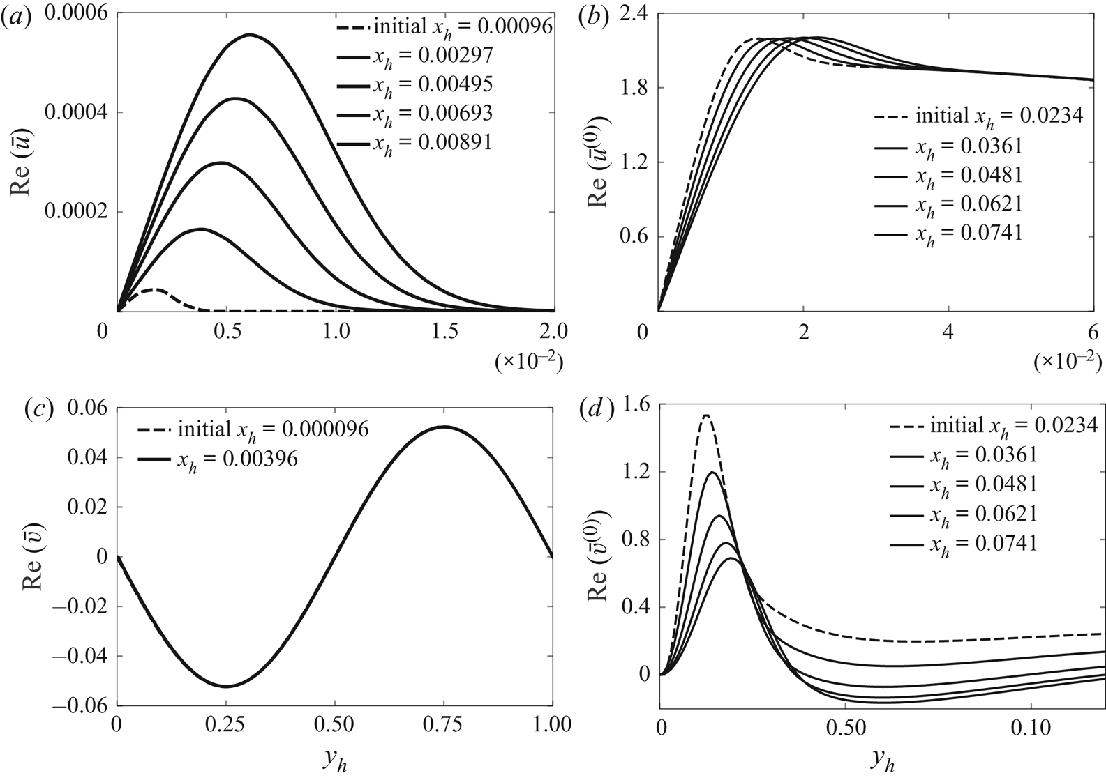
The appropriate specification of the composite initial condition requires a smooth matching with the numerical solutions of the boundary-region equations (2.21) and (2.22) at small  $x_h$ locations. This matching is monitored by comparison in figure 5. Figure 5 shows that the asymptotic profiles (dashed lines), used as initial conditions for the numerical integration of the boundary-region equations, are consistent with the numerical solutions (solid lines) at small
 $x_h$. The streamwise
 $\bar {u}$ profiles resemble the profiles of the Klebanoff modes appearing in free-stream open boundary layers (shown in figure 3 on page 184 of LWG99), although the peak of the numerical profiles is slightly closer to the channel centreline. The confinement of the channel has an influence on the amplitude and growth rate of
 $\bar {u}$ through
 $\bar {w}_{com}$, given in (3.9), because
 $\bar {w}_{com}$ depends on
 $h$.
Real parts of the streamwise and wall-normal velocity components for the reference conditions of table 1 generated by an oncoming symmetric-gust disturbances, i.e.  $\hat {u}^\infty _{x,y,\pm }=1.0, \hat {u}^\infty _{z,\pm }=1.0$. The solid lines indicate the numerical solutions of the boundary-region equations (2.21) and (2.22) and the dashed lines indicate the asymptotic composite solutions used as initial conditions of the numerical calculations: (3.11) for
 $\bar {u}$, (3.13) for
 $\bar {u}^{(0)}$, (3.12) for
 $\bar {v}$ and (3.18) for
 $\bar {v}^{(0)}$.

As evident from the top graphs of figure 5, at these locations the dominant part of the total streamwise disturbance velocity  $\bar {u}_0$ is due to
 $\bar {u}^{(0)}$, which is given in (3.13) and is caused by the direct free-stream forcing action of the inviscid streamwise velocity in (3.5). The part due to
 $\bar {u}$ is smaller, which means that the streaks have not formed yet and do not dominate the boundary layers over the channel walls.
4.2. Reference perturbation flow in regions V and VI
The downstream evolution of the disturbance field for the conditions of table 1 is investigated for the cases of perturbations at the channel entrance that are symmetric ( $\hat {u}^\infty _{x,z,\pm }=1.0$) and anti-symmetric (
 $\hat {u}^\infty _{x,z,+}=1.0, \hat {u}^\infty _{x,z,-}=-1.0$) with respect to the channel centreline. The inflow perturbations are streamwise-stretched vortices that are round in cross-sectional
 $y-z$ planes because the spanwise and the wall-normal wavelengths are equal and much shorter than the streamwise wavelength. As discussed in § 2.3, at this bulk Reynolds number,
 $R_h=1500$, no TS-waves exist, but nevertheless an intense transient growth is detected. This growth is monitored by the energy of the perturbation, defined as
 \begin{equation} \mathcal{E}(x_h) = \underbrace{\frac{1}{2} \int_0^2 |\bar{u}_0|^2 \, \mathrm{d} y_h}_{\mathcal{E}_u} + \underbrace{\frac{1}{2} \int_0^2 |\bar{v}_0|^2 \, \mathrm{d} y_h}_{\mathcal{E}_v} + \underbrace{\frac{1}{2} \int_0^2 |\bar{w}_0|^2 \, \mathrm{d} y_h}_{\mathcal{E}_w},\end{equation}
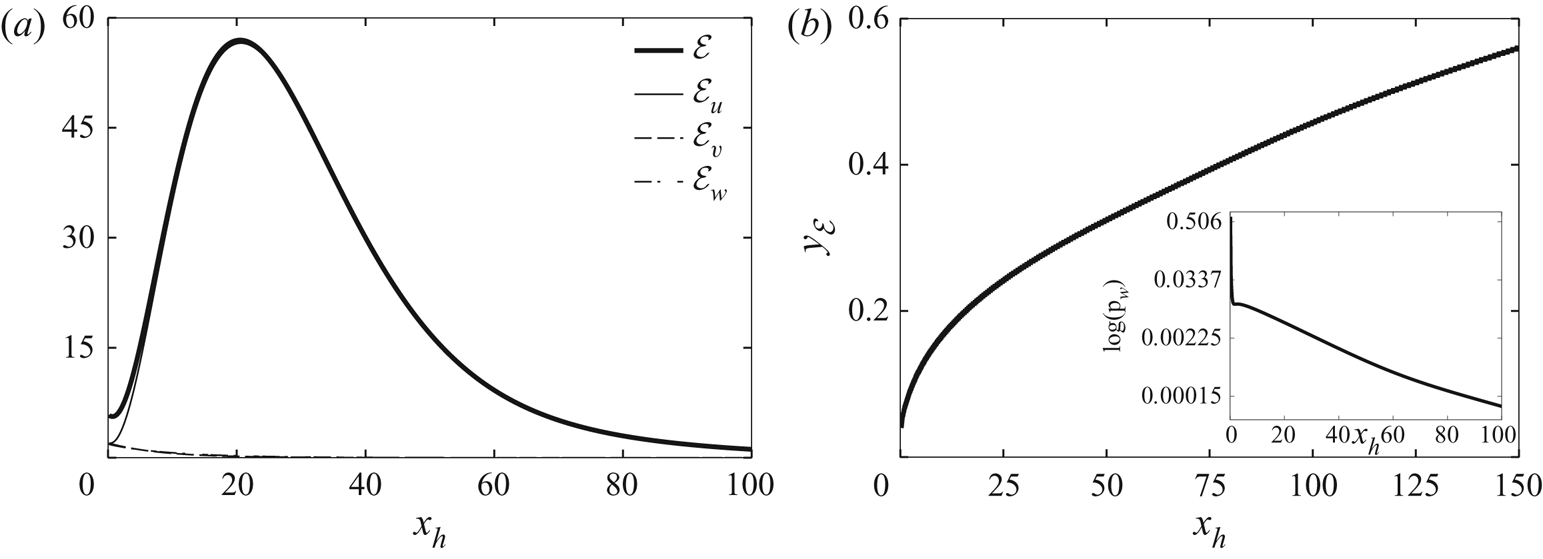
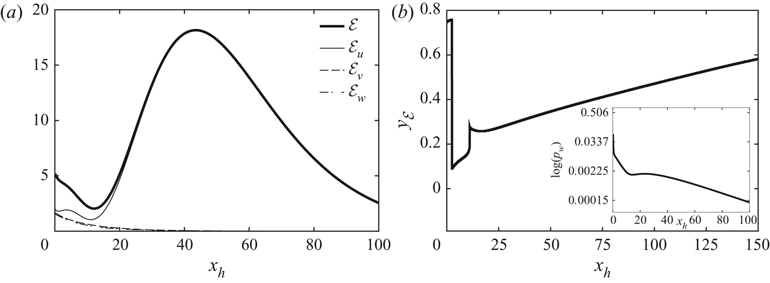
where the velocity components  $\bar {u}_0, \bar {v}_0, \bar {w}_0$ are defined in (2.9). Figure 6(a) shows that, while at the entrance the three velocity components have the same intensity, the streamwise velocity component generated by a symmetric-gust disturbance is the major contributor to the perturbation dynamics as the total energy grows from the channel inlet, while the other two velocity components decay at the same rate. Downstream of
 $x_h=20$, the total energy is almost entirely due to
 $\bar {u}_0$ and it decreases due to viscous effects. The entrance region, estimated through the centreline base-flow velocity, terminates at
 $x_h=258$ and therefore the transient growth is wholly confined in region V, upstream of the fully developed region VI.
(a) Streamwise evolution of the perturbation energy  $\mathcal {E}$ and of its three parts
 $\mathcal {E}_u, \mathcal {E}_v, \mathcal {E}_w$ related to the velocity components. (b) Streamwise evolution of the wall-normal location of the maximum
 $\mathcal {E}$ and of the amplitude of the wall perturbation pressure
 $p_w$ (inset). All trends are for the case of a symmetric-gust disturbance.

Figure 6(b) reveals that most of the perturbation energy is confined within the boundary layers as the wall-normal location  $y_{\mathcal {E}}$ of the maximum energy
 $\mathcal {E}$ is smaller than the boundary-layer thickness
 $\delta _h$, depicted in figure (S5)(left). The inset of figure 6(b) displays the downstream evolution of the magnitude of the pressure at the wall, i.e.
 \begin{equation} p_w(x_h) = |\bar{p}_0(y_h=0)| = k_{zh}^{{-}2} \biggm\lvert \frac{\partial^2 \bar{w}_0}{\partial y_h^2}\biggm\lvert_{y_h=0}, \end{equation}
where the relation to the spanwise velocity is found from (2.25). It decays monotonically, sharply up to  $x_h=2$ and more mildly further downstream.
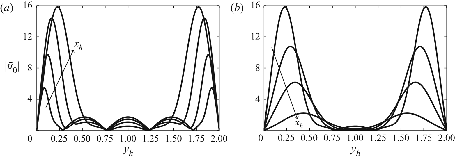
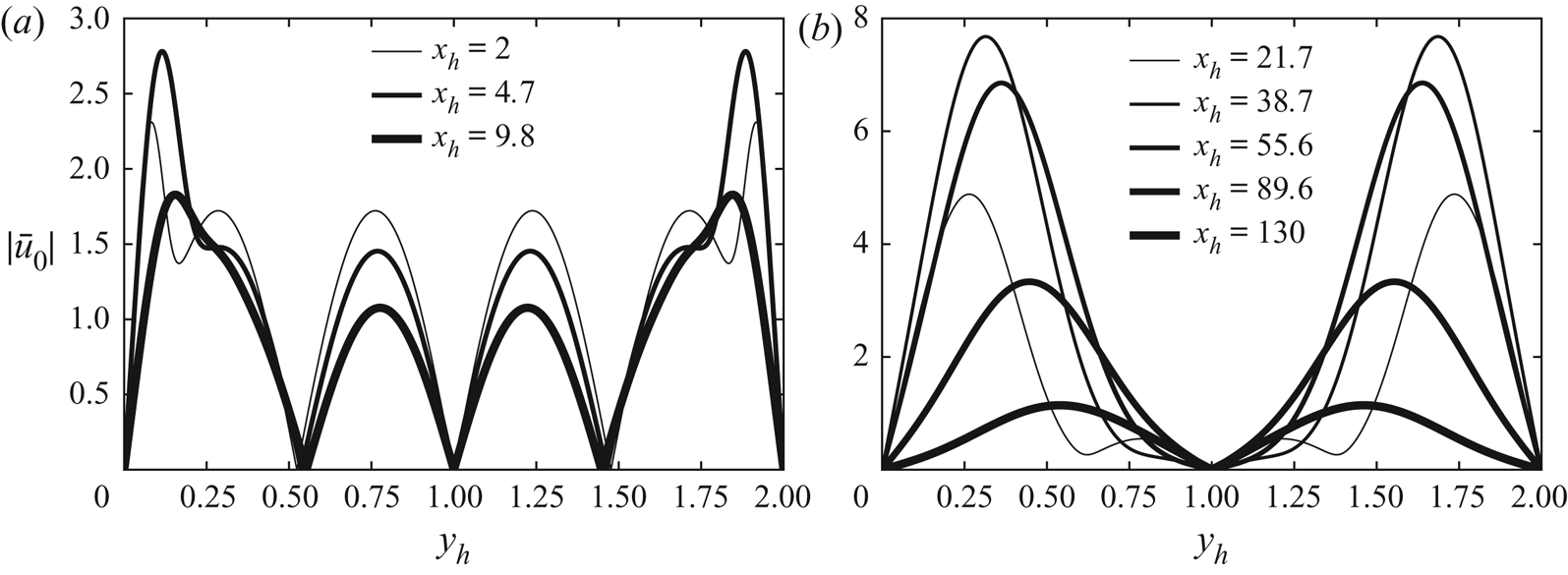
The wall-normal profiles of  $|\bar {u}_0|$ are shown in figure 7 (panel (a) for growing disturbances and (b) for decaying disturbances). The disturbance near the centreline always decays because of the almost total absence of base-flow velocity gradients that instead enhance the intensity of the perturbation near the walls. The maximum of
 $|\bar {u}_0|$ moves towards the centreline at all streamwise locations. The spanwise velocity
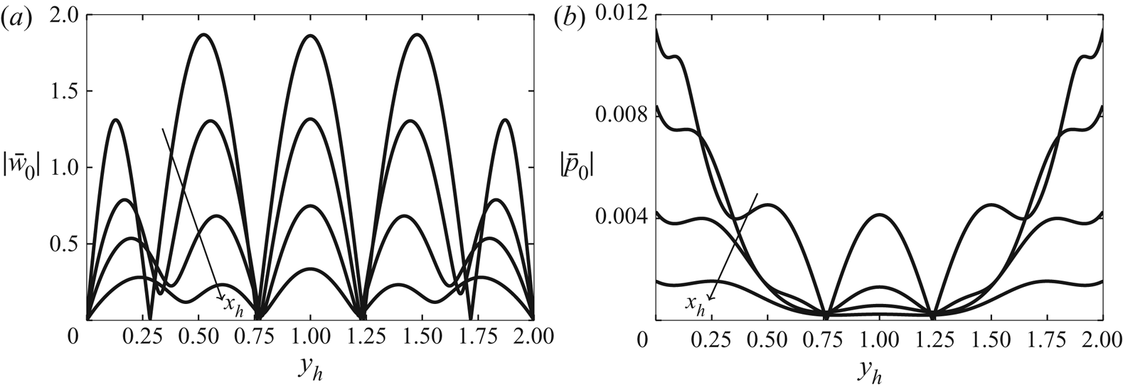
 $|\bar {w}_0|$ in figure 8(a) decays almost at the same rate irrespectively of the wall-normal location and so does the wall-normal velocity
 $|\bar {v}_0|$ (not shown). Figure 8(b) confirms that the pressure
 $|\bar {p}_0|$ is related to
 $|\bar {w}_0|$ as they share the same locations of the maxima, although the overall maximum pressure disturbance is found at the wall.
Wall-normal profiles of the streamwise velocity amplitude  $|\bar {u}_0|$ at different streamwise locations for the case of a symmetric-gust disturbance. (a) growing disturbances at
 $x_h=2, 4.7, 9.8, 21.7$. (b) decaying disturbances at
 $x_h=21.7, 38.7, 55.6, 89.6$.

Wall-normal profiles of the spanwise velocity amplitude  $|\bar {w}_0|$ (a) and of the pressure amplitude
 $|\bar {p}_0|$ (b) at
 $x_h=2, 9.8, 21.7, 38.7$ generated by a symmetric-gust disturbance.

The flow dynamics triggered by the anti-symmetric-gust disturbance imposed at the channel entrance presents notable differences from the one of the symmetric disturbance. Figure 9(a) shows that, while the total energy is still primarily due to  $|\bar {u}_0|$, the streamwise velocity oscillates mildly up to
 $x_h=5$, decays up to
 $x_h=12$, and then grows to a maximum that is only approximately a third of the one attained by the flow forced by the symmetric-gust disturbance. This maximum also occurs at double the distance of the symmetric-gust flow. The cross-flow velocity components decay as in the symmetric-gust case. In figure 9(b), the maximum energy location
 $y_{\mathcal {E}}$ is confined within the boundary layers, except in the proximity of the channel entrance. The trend is not continuous because different local maxima emerge as the global maximum during the downstream flow evolution.
(a) Streamwise evolution of the perturbation energy  $\mathcal {E}$ and of its three parts
 $\mathcal {E}_u, \mathcal {E}_v, \mathcal {E}_w$ related to the velocity components. (b) Streamwise evolution of the wall-normal location of the maximum
 $\mathcal {E}$ and of the amplitude of the wall perturbation pressure
 $p_w$ (inset). All trends are for the antisymmetric-gust case.

The streamwise oscillatory behaviour near the channel inlet occurs within the boundary layers, while the perturbation in the channel core decreases monotonically, as shown in figure 10(a). During the growth and subsequent decay (figure 10b), the wall-normal  $|\bar {u}_0|$ profiles resemble the decaying perturbations in figure 7(b).
Wall-normal profiles of the streamwise velocity amplitude  $|\bar {u}_0|$ for the case of the antisymmetric-gust disturbance at different streamwise locations.

4.3. Effect of Reynolds number
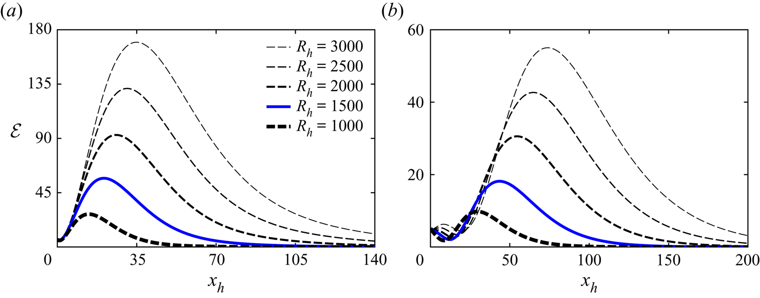
The change of the downstream evolution of the total energy  $\mathcal {E}$ as the bulk Reynolds number
 $R_h$ varies is shown figure 11 for the symmetric-gust case (a) and the anti-symmetric-gust case (b). As
 $R_h$ increases, the energy generated by the symmetric gust at the channel entrance is initially largely unaffected up to approximately
 $x_h=5$, while the energy of the anti-symmetric disturbance decays up to approximately
 $x_h=15$ for
 $R_h\leq 2000$ and oscillates spatially up to approximately
 $x_h=20$ for
 $2500< R_h<3000$. This initial oscillatory behaviour is due to the streamwise velocity component as the cross-flow velocities decay monotonically. It is a peculiar feature of the response of the channel-entry shear layers to oncoming vortical disturbances because it does not occur in unconfined boundary layers exposed to free-stream disturbances (LWG99). Further downstream the disturbance energy increases monotonically with
 $R_h$ and the maximum occurs at larger streamwise locations as
 $R_h$ increases. This dependence on the Reynolds number also occurs in open boundary layers exposed to free-stream vortical structures and the scaled spanwise wavenumber
 $\kappa =k_z/(k_x R_\lambda )^{1/2}$ is the governing parameter, as shown by LWG99. In LWG99's figures 5 and 6, as
 $\kappa$ decreases from 1 to 0.1 the streamwise velocity, which dominates the total energy, increases and its maximum occurs further downstream. This result is consistent with the cases of figure 11, for which
 $\kappa$ decreases in the range
 $0.33<\kappa <0.58$ as
 $R_h$ increases. The wall-normal locations of the energy maxima move closer to the walls at larger
 $R_h$ as the boundary layers becomes thinner (not shown).
Effect of  $R_h$ on the downstream evolution of total energy
 $\mathcal {E}$ for the symmetric-gust case (a) and the anti-symmetric-gust case (b). The blue solid line in this figure and in figures 13, 15 and 14 indicates the reference case of table 1.

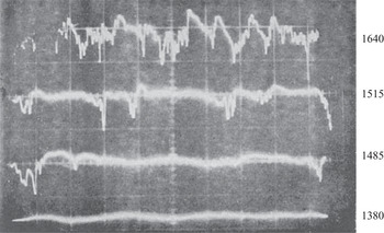
Some qualitative confirmation of the enhancement of the perturbation intensity as the Reynolds number increases is given by the traces of hot-wire measurements reported by Patel & Head (Reference Patel and Head1969) and shown in figure 12. The air flow was measured at a distance of 203 channel heights from the entrance ( $x/h=406$), at which the flow reached its fully developed parabolic profile for the Reynolds numbers
 $2 Re_h$ given on the right of the images. The perturbations at that downstream location were generated by fluctuations at the entrance of the channel. The air flow was sufficiently disturbed at the channel entrance to become more unstable further downstream as the Reynolds number increased, as predicted by the theoretical results shown in figure 11, despite being linearly stable according to classical stability theory. As Patel & Head's (Reference Patel and Head1969) measurements were conducted in the fully developed region, experimental data and nonlinear numerical data in the channel-entrance region are needed for a more meaningful comparison.
Subcritical enhancement of air-flow perturbations caused by vortical disturbances at the entrance of a channel (Patel & Head Reference Patel and Head1969). The number on the right is the Reynolds number  $2 Re_h$.

4.4. Effect of streamwise wavelength
The change of the streamwise wavelength  $\lambda _{xh}$ of the oncoming disturbance is inversely proportional to the frequency as the two quantities are related through the free-stream velocity
 $U_\infty ^*$ for small-amplitude free-stream convective gusts. As evident in figure 13, the initial energy amplitude is independent of
 $\lambda _{xh}$ as this parameter does not appear in the velocity components in (2.3) and (2.4). At streamwise distances up to
 $x_h=10$ for both cases,
 $\lambda _{xh}$ has no influence on the disturbance growth as all the profiles collapse on one another. Further downstream, oncoming disturbances with longer wavelengths (smaller frequencies) grow more energetically and their maxima occur at larger streamwise locations. The trends at the two highest
 $\lambda _{xh}$ overlap (solid red line and dashed white line), showing the independence of the dynamics from the frequency.
Effect of  $\lambda _{xh}$ on the downstream evolution of total energy
 $\mathcal {E}$ for the symmetric-gust case (a) and the anti-symmetric-gust case (b).

Luchini (Reference Luchini2000) also predicted the optimal perturbations to be steady, although in that case free-stream vortical disturbances were absent and the perturbations were solely confined within the boundary layer (Andersson et al. (Reference Andersson, Berggren and Henningson1999) assumed the perturbations to be steady). However, the results of the most detrimental perturbation being steady can be misleading because our results in figure 13 show that oncoming perturbations with measurable unsteadiness, i.e. with frequency  $f^*=2$ Hz (
 $\lambda _{xh}=100$) for the air channel in table 1, may be equally likely to lead to the flow breakdown as they achieve a growth which is very close to the optimal one.
The asymptotic scaling at large  $\lambda _{xh}$ can be studied by use of
 $\epsilon = k_{xh}R_h \ll 1$, where
 $k_{xh}=2 {\rm \pi}/\lambda _{xh}$. The base-flow equations (2.11) and (2.10) rescale as
 $$\begin{gather} U\frac{\partial U}{\partial \hat x}+\hat V\frac{\partial U}{\partial y} ={-}\frac{\text{d} P}{\text{d} \hat x} + \hat \gamma \frac{\partial^2 U}{\partial y^2}, \end{gather}$$
 $$\begin{gather}\frac{\partial P}{\partial y}=0, \quad \frac{\partial U}{\partial \hat x}+\frac{\partial \hat V}{\partial y}=0, \end{gather}$$
where  $\hat V = \epsilon V, \hat x = x_h/R_h$ and
 $\hat \gamma = (k_{zh}/2 {\rm \pi})^2 = O(1)$. In the limit
 $\epsilon \rightarrow 0$, the boundary-region equations (2.21) and (2.22) reduce to
 \begin{align} &\left({-}k_z^2 k_{zh}^2 - k_z^2 \frac{\partial \hat V}{\partial y}+\frac{\partial^3 \hat V}{\partial y^3}\right)\bar{v}- \left(k_z^2 \hat V - \frac{\partial^2 \hat V}{\partial y^2} \right) \frac{\partial \bar{v}}{\partial y} +\left(2 k_{zh}^2 + \frac{\partial \hat V}{\partial y} \right)\frac{\partial^2 \bar{v}}{\partial y^2}\nonumber\\ &\quad + \hat V \frac{\partial^3 \bar{v}}{\partial y^3} +U\frac{\partial^3 \bar{v}}{\partial \hat x\partial y^2} -\hat \gamma \frac{\partial^4 \bar{v}}{\partial y^4} -\left(k_z^2 U + \frac{\partial^2 U}{\partial y^2} \right)\frac{\partial \bar{v}}{\partial \hat x} -\left(k_z^2 \frac{\partial \hat V}{\partial \hat x}-\frac{\partial^3 \hat V}{\partial \hat x \partial y^2}\right)\hat u\nonumber\\ &\quad -2\frac{\partial^2 U}{\partial \hat x\partial y}\frac{\partial \hat u}{\partial \hat x} -2 \frac{\partial U}{\partial \hat x}\frac{\partial^2 \hat u}{\partial \hat x \partial y}-\frac{\partial \hat V}{\partial \bar{x}}\frac{\partial^2 \hat u}{\partial y^2}=0, \end{align}
 \begin{align} &\left( k_{zh}^2 +\frac{\partial U}{\partial \hat x} \right)\hat u + U \frac{\partial \hat u}{\partial \hat x} + \hat V \frac{\partial \hat u}{\partial y} - \hat \gamma \frac{\partial^2 \hat u}{\partial y^2} + \frac{\partial U}{\partial y}\bar{v}=0, \end{align}
where  $k_{zh}=2 {\rm \pi}h^*/\lambda _z^*$ and
 $\hat u = \bar {u}/\epsilon$. All the terms in (2.21) and (2.22) that are proportional to
 $i$, which arise due to the unsteadiness of the oncoming disturbance (2.1), do not appear in (4.5) and (4.6) because the low-frequency disturbance dynamics is now steady at leading order. The analogous scaling for open free-stream boundary layers was first found by LWG99 on pages 183–185. In figure 13, the behaviour is consistent with the asymptotic analysis for
 $\epsilon \ll 1$:
 $R_h$ is constant for those cases and thus it does not impact on the streamwise scaling
 $\hat x$, and at leading order the total energy is
 \begin{equation} \mathcal{E} \sim \frac{1}{2}\int_0^{2} \biggm\lvert\frac{k_z}{k_x} \hat u \biggm\lvert^2 \, \mathrm{d} y_h = \frac{k_{zh}^2 R_h^2}{2}\int_0^{2} |\hat u |^2 \, \mathrm{d} y_h, \end{equation}
which is independent of  $\lambda _{xh}$.
4.5. Effect of wall-normal wavelength
Figure 14 shows that the transient growth decreases as the wall-normal wavelength of the oncoming disturbance becomes smaller. This result is due to the more intense viscous dissipation caused by the high velocity gradients at small wavelengths. Therefore the most energetic growth occurs for the largest wavelength, i.e. when  $\lambda _y^*$ spans the whole channel height (
 $\lambda _{yh}=2$). For our choice of specified disturbances in (2.3), i.e. with fixed
 $\hat u_{x,z,\pm }^\infty$ and wavelengths, the initial amplitude of
 $u_y$ increases proportionally to
 $\lambda _{yh}$ to maintain the solenoidal condition (2.2) at the channel entrance. However, this change of
 $u_y$ is not the reason for the intense growth at larger
 $\lambda _{yh}$ because the disturbance amplifies more than the linear increase proportional to
 $u_y$. For wavelengths
 $\lambda _y^*$ that are one fifth (
 $\lambda _{yh}=2/5$) or shorter than the channel height, no downstream growth of the symmetric disturbance is detected because of viscous effects, while the attenuation is less effective on the anti-symmetric disturbance. The location of the maximum energy is found to be closer to the channel entrance as
 $\lambda _{yh}$ drops.
Effect of  $\lambda _{yh}$ on the downstream evolution of total energy
 $\mathcal {E}$ for the symmetric-gust case (a) and the anti-symmetric-gust case (b).

An important observation is that the effect of  $\lambda _{yh}$ on the disturbance evolution cannot be investigated through the non-normality of the eigenfunctions of the developing boundary layers on the channel walls. This limitation occurs because an eigenvalue-based approach would model the near-entrance disturbance as wholly confined within the near-wall boundary layers, whereas
 $\lambda _{yh}$ is a parameter that solely pertains to the oncoming external flow and does not enter the classical stability problem of the boundary layer. The spanwise and the streamwise wavelengths can instead enter the eigenvalue problem directly because the base flow is spanwise independent and steady. The boundary-region approach based on (2.21)-(2.22) can account for the characteristics of the oncoming flow because it is an initial-value problem where the specification of the oncoming disturbances at the channel entry is crucial for the flow dynamics downstream.
4.6. Effect of spanwise wavelength
The influence of the variation of the spanwise wavelength  $\lambda _{zh}$ is shown in figure 15. There exists an optimal
 $\lambda _{zh}$ (the reference
 $\lambda _{zh}=1$ for the symmetric disturbance and
 $\lambda _{zh}=2$ for the antisymmetric disturbance) that leads to the most energetic growth. Disturbances with very small
 $\lambda _{zh}$ are strongly influenced by viscous dissipation that hampers their growth. Oncoming disturbances with large spanwise wavelength,
 $\lambda _{zh}=4,8$ are almost two-dimensional and, although they do not produce the maximum growth, they persist further downstream because they are less affected by viscous dissipation due to spanwise shear effects. The perturbations with the largest tested wavelength,
 $\lambda _{zh}=16$, decay monotonically, confirming that the transient streaky growth is a three-dimensional phenomenon.
Effect of  $\lambda _{zh}$ on the downstream evolution of total energy
 $\mathcal {E}$ for the symmetric-gust case (a) and the anti-symmetric-gust case (b).

5. Conclusions
In this paper we have presented a theoretical and numerical analysis of the entrainment and growth of unsteady three-dimensional vortical disturbances in the entrance region of pressure-driven incompressible plane channel flows, as steps towards the full comprehension of laminar to turbulent transition in confined flows. The focus is on a Reynolds number range where experimental evidence has documented the occurrence of intense transient growth, despite the flow being stable when studied through classical stability analysis.
The mathematical approach is based on the method of matched asymptotic expansions and on the assumption of high Reynolds number, and is pertinent to naturally present and physically realizable free-stream perturbations. The low-frequency assumption has been motivated by the ample evidence that these disturbances amplify the most in open free-stream boundary layers to form transition-triggering Klebanoff modes. This framework has allowed for a precise analytical description of the base flow and of realistic vortical perturbations that can be created in a laboratory set-up at the channel mouth. The effects of the channel confinement, the streamwise pressure gradient and the viscous/inviscid interplay have been revealed through the analysis. We have shown how the amplitude of the initial disturbance is not arbitrary, but is instead uniquely related to, and amplified from, the one of the oncoming free-stream perturbation. The wall-normal transpiration effect of the perturbation from the boundary layer is the source of the second-order perturbations in the inviscid core. Furthermore, the composite velocity profiles of both the base flow and the disturbance flow have served the purpose of rigorous initial conditions for the parabolic base-flow boundary-layer equations and the boundary-region perturbation equations. The latter equations have been cast in a numerically efficient vertical velocity and vertical vorticity formulation containing extra terms with respect to the classical Orr–Sommerfeld/Squire equations because of the non-negligible influence of non-parallel effects.
The base-flow quantities agree with results from direct numerical simulations and experiments, and we have found that monitoring the second derivative of the base flow at the channel centreline is the most conservative method for quantifying the length of the entrance region. A complete parametric study has been carried out on the perturbation flow where the base flow departs significantly from the Blasius self-similar form and is thus fully influenced by the streamwise pressure gradient, the wall-normal velocity component and the confinement of the channel walls. In the proximity of the channel mouth where the base-flow pressure gradient plays a minimal role, the disturbance flow is most dominant within the boundary layers attached to the channel walls because of the shear-driven amplifying effect responsible for the formation of the streamwise-elongated streaks. As the wall confinement becomes paramount the viscous disturbances permeate the whole channel, although the base flow is still mostly inviscid in the core. For all the tested cases, the intense transient growth and the subsequent decay are always detected in the entrance region, i.e. where the base flow has not reached the parabolic Poiseuille profile. A pressing issue is thus to test the effect of nonlinearity on this result, that is, to verify whether nonlinear vortices may persist downstream of the entrance region. We further find that symmetrical disturbances exhibit a more significant growth than anti-symmetrical disturbances for the same frequency and wavelengths. The latter can linger for several channel heights downstream before displaying the transient growth, a unique feature that has never been detected in open free-stream boundary layers. The disturbance growth is intensified as the frequency decreases and the bulk Reynolds number and the wall-normal wavelength increase. The spanwise wavelengths that cause the most intense downstream growth are computed.
We plan to extend our work to include a full spectrum of oncoming disturbances and to relax the assumption of small amplitude to study the nonlinearly evolving flow and its secondary instability. A next step will be to provide a robust inlet flow field for direct numerical simulations with the aim of investigating the fully fledged transitional flow. A central objective is certainly to predict the transition location as a function of the characteristics of the oncoming vortical flow at the channel mouth.
Supplementary material
Supplementary material are available at https://doi.org/10.1017/jfm.2021.765.
Acknowledgements
We are indebted to Dr V. Nguyen from the Institute of High Performance Computing in Singapore and to Professor X. Wu from Imperial College London for the interesting discussions about our work.
Funding
The authors would like to thank the A*STAR-Sheffield Research Attachment Programme and the University of Sheffield for funding this research.
Declaration of interests
The authors report no conflict of interest.