Research sites, animals and dates of study

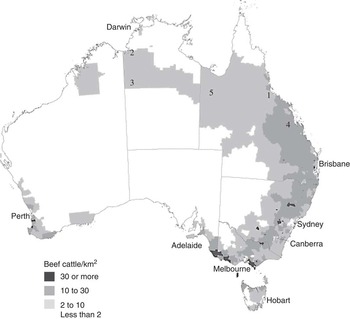
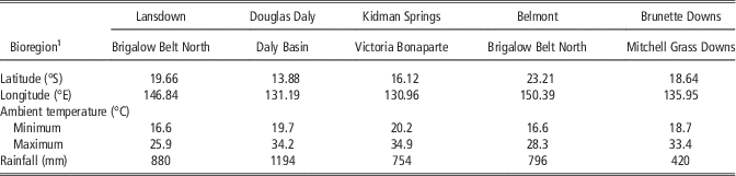
Five research sites were selected and measurements made over a 3-year period from 2010 to 2012 (Figure 1, Table 1). The sites were chosen so as to be representative of the dominant beef grazing areas of northern Australia and reflect a range of stocking densities and bioregions (Interim Biogeographic Regionalisation for Australia, 2012).

Figure 1

Map of Australia showing approximate locations where measurements were taken and cattle density in 2001 (Australian Bureau of Statistics, 2005).1 Lansdown Research Station; 2 Douglas Daly Research Station; 3 Kidman Springs Research Station; 4 Belmont Research Station; 5 Brunette Downs.

Table 1

Geographical location of the study sites and their mean (100 year average) annual climate conditions

¹ Interim Biogeographic Regionalisation for Australia, version 7 (2012).

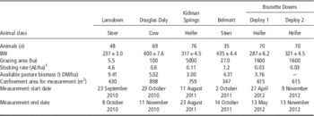
Descriptions of the cattle, grazing conditions and timing of measurements are given in Table 2. Cattle at all sites were weighed before and after the CH₄ measurements and a mean BW used to estimate stocking density and CH₄ emissions as g/kg BW. Pasture biomass and botanical composition was estimated using a modification of the ‘Botanal’ method described by Tothill et al. (Reference Tothill, Hargreaves, Jones and McDonald1992).

Table 2

Description of the study areas, animals and pastures used in the research

¹ AE (adult equivalent)=450 kg steer.

The CSIRO Lansdown Research Station near Townsville in north Queensland represented the Northern Brigalow Belt bioregion. This first study was designed to test the method under controlled conditions. CH₄ emissions were measured in beef steers; 15 Brahman (Bos indicus) and 33 Belmont Red (Bos taurus×African Sanga), continuously grazing a 5.5 ha established mixed sward of (~67%) sabi grass (Urochloa mosambiensis), (~18%) Siratro sp., (~10%) Stylosanthes sp. with some blue pea (Clitoria turnatea) and green panic (Panicum maximum). CH₄ measurements were made in the mid to late dry season (September to October) 2010. Following this deployment, laser CH₄ measurements were conducted under extensive grazing conditions at the Northern Territory Government Department of Resources Douglas Daly Research Farm in the Daly Basin in October to November during the late dry season. CH₄ emissions were recorded in Brahman and Brahman cross cows grazing a 100 ha pasture containing (~48%) buffel grass (Cenchrus ciliaris), (~35%) sabi grass (U. mosambiensis) and (~14%) wynn cassia (Chamaecrista rotundifolia).

Two studies were conducted in the dry season (August and October) of 2011. The first of these at the Kidman Springs Research Station in the Northern Territory, represented the Victoria Bonaparte bioregion. This region has a hot, seasonally dry monsoonal climate, with most rain falling between December and March. Measurements were taken from Brahman×Senepol cross heifers, continuously grazing a 5000 ha native pasture consisting of open woodland of Bauhinia sp. with an understorey of native couch (Brachyachne convergens), golden beardgrass (Chrysopogon fallax) and occasional mitchell grass (Astrebla sp.) patches. In October 2011, measurements were conducted at the Belmont Research Station near Rockhampton in coastal central Queensland. This land type represented the southernmost extent of the Northern Brigalow Belt bioregion noted for superior pasture and livestock performance compared with other bioregions in the north. Measurements were conducted on a herd of 35 Brahman steers (mean±SEM BW of 435±4.4 kg) continuously grazing a 27 ha established mixed sward. The sward consisted of (~18%) Rhodes grass (Chloris gayana), (~16%) sabi grass and (~15%) Bothriochloa sp. with some Black speargrass (Heteropogon contortus) and (<15%) introduced tropical grasses.

In 2012, two deployments were conducted on the Australian Agricultural Company Ltd (AACo) property, Brunette Downs in April (early dry season) and October (late dry season). This property was selected to represent the Mitchell Grass Downs bioregion typified by open rolling grasslands. On both occasions CH₄ emissions were measured using the same herd of AACo Composite heifers (Senepol×Charolais×Santa Gertrudis), continuously grazing an unimproved pasture (1600 ha) dominated by hoop michell grass (Astrebla elymoides) and barley mitchell grass (Acianthera pectinata) with some Flinders grass (Iseilema sp.). On both occasions animals grazed the same paddock and samples of available pasture were collected along three transects radiating from the water point.

CH₄ measurements

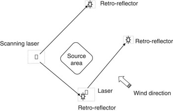
Under extensive grazing situations, cattle are dispersed widely across large areas, conditions unsuited to laser measurements. However, observational data has shown that cattle congregate in groups around water points during the daytime. We exploited this behaviour by confining cattle in defined areas around water points to facilitate measurements using the backward Lagrangian stochastic (BLS) dispersion model (Flesch et al., Reference Flesch, Wilson, Harper and Crenna2004 and 2005). In these studies it was assumed that the area represented a uniform source of CH₄ (Figure 2).

Figure 2

Schematic diagram of laser deployment. Dashed boxes represent fenced off areas for protection of equipment.

The methods employed were based on those developed in earlier studies by Tomkins et al. (Reference Todd, Altman, Cole and Waldrip2011) and McGinn et al. (Reference McGinn, Turner, Tomkins, Charmley and Chen2011). CH₄ concentration from each group of cattle at each of the field sites were measured by OPL (GasFinder 2.0; Boreal Laser Inc., Spruce Grove, Alberta, Canada) for 6 to 7 h/day for up to 16 days (Figure 2). Following morning grazing animals were confined to an area (Table 3), established around the only water point in the study paddock. This confinement assumes a uniform distribution of animals within the area and surface-source assumptions were used in a BLS dispersion model to derive CH₄ flux (McGinn et al., Reference McGinn, Flesch, Coates, Charmley, Chen, Bai and Bishop-Hurley2015). The surrounding area at each site was flat and considered to present no major impediments to wind characteristics.

Table 3

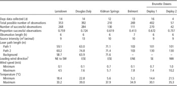
Description of the open-path laser characteristics used at six study areas in northern Australia

¹ NE=north-east, SW=south-west, ESE=east-south-east, ENE=east-north-east, SE=south-east, NW=north-west.

In five of the six campaigns, two OPL were used to measure line-averaged CH₄ mixing ratio for each path; one set upwind to measure the background CH₄ mixing ratio and another mounted on a motorised scanner measured line-averaged CH₄ mixing ratios from the source area along two perpendicular paths. The physical arrangement of equipment at each site was determined by historical meteorological data for wind direction to ensure that paths were predominantly measuring background or enhanced CH₄ flux relative to each source area. Retro reflectors were used to terminate each laser path with lengths ranging from 59 to 144 m (Table 3). Path lengths unique to each measurement campaign were used in BLS modelling to estimate herd-scale emission values. For the Belmont campaign in October 2011, only one OPL was available. This laser was mounted on a scanner and measured line averaged background CH₄ mixing ratio and CH₄ mixing ratios from the source area along two paths ±19.2° relative to a centre line between the scanner and centre of the source area.

Before each campaign, in the absence of animals, continuous line averaged concentration data was collected for each OPL along parallel paths for cross-calibration purposes. This allowed for direct calibration between the two sensors and generated a correction factor which was applied to data collected for each independent measurement period. This protocol developed multipliers for each measurement campaign to force the line averaged concentration of multiple laser paths to match that of the standalone laser used at that time. In principle this is a good approach as it eliminates systematic measurement errors due to errors in the measured laser path lengths, the possibility of errors due to different laser signal levels on the different paths and reflector differences (Flesch, T.K., personal communication). Harper et al. (Reference Harper, Flesch, Weaver and Wilson2010) includes an appendix tabulating several WindTrax verification studies and indicates that the period-to-period relative uncertainty in a WindTrax calculation is 0.20 (given by the standard deviation of the fractional uncertainty in the various experimental datasets). Therefore, given the commonalities in the open-path methodology we assume a similar relative uncertainty; δK/K=0.20. Recording interval for line-averaged CH₄ mixing ratio (ppm) for all paths was every second for 60 s. CH₄ mixing ratios from each OPL for each campaign was averaged over 10-min periods. Laser return light levels were also checked throughout each campaign to ensure values between 3000 and 11 000 (no units). This range is recommended by the manufacturer and associated CH₄ concentration readings can be considered reliable.

At each site a micrometeorological tower was located upwind and adjacent to each source area (Figure 2). The tower was fitted with a three-dimensional sonic anemometer (CSAT3; Campbell Scientific Inc., Logan, UT, USA) mounted at a height of 2.4 m which sampled wind components at 10 Hz. A barometric pressure sensor (CS106, PTB 110; Campbell Scientific Inc.), temperature humidity sensor (HMP45C; Campbell Scientific Inc.), and a 3-cup anemometer and wind vane mounted on a small cross arm (03002-L; Campbell Scientific Inc.) were also mounted on the tower. Micrometeorological data including wind speed, direction and wind component variance were recorded at 10 Hz, averaged over 10 min intervals using a data logger (CR1000; Campbell Scientific Inc.) and all records were extracted daily onto a laptop computer.

Data processing

Laser, sonic anemometer and micrometeorological data were merged and managed with SAS (1999) statistical software as described by Tomkins et al. (Reference Todd, Altman, Cole and Waldrip2011) before using BLS modelling in WindTrax (WindTrax dispersion model V.2.0.8.3; Thunder Beach Scientific, Halifax, NS, Canada). The location, by GPS, of source boundaries and sensors is also required in this model to provide relative spatial orientation of the source area to individual sensors and measurement paths so that assumptions based on wind direction can be validated. In addition, unique to each site is the use of an offset value in cardinal degrees relative to true north (0 to 360°) which is applied to sonic anemometer data. The filtering criteria used throughout the studies for pre- and post-simulation (using WindTrax) were similar to that described by Flesch et al. (Reference Flesch, Wilson, Harper, Crenna and Sharpe2007) and McGinn et al. (Reference McGinn, Beauchemin and Flesch2009) and included; 3000<light level<11 000, surface roughness (Z; m) 0.0000001<Z ₀<0.9, atmospheric stability (L; m), absolute <2, friction velocity (u*; m/s) >0.15 m/s, where <0.15 indicates calm conditions and unsteady wind directions, and fraction covered by touchdown >10% with ∆CH₄>10 ppb. In addition, if the wind direction relative to either path varied by >15° then these data was considered unreliable and excluded from modelling. The CH₄ mixing ratio for each path was converted to an absolute concentration based on air pressure and temperature. Individual 10 min data points were plotted against time for each site. Mean individual animal (within a herd) CH₄ emission were then calculated (g/day) for each study site based on the total number of 10 min average data that satisfied the filtering criteria as described and the number of animals confined in that source area.

Mean CH₄ emissions

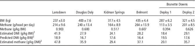
Table 4 summarises the CH₄ emission estimates for the six deployment campaigns. Except for the Lansdown site, CH₄ emissions expressed on a BW basis varied between 0.39 and 0.63 g/kg BW, which is in agreement with emission values previously reported using similar methodology (Tomkins et al., Reference Todd, Altman, Cole and Waldrip2011). The mean emission value for the Lansdown site was 0.90 g/kg BW, which is outside the expected range. Kennedy and Charmley (Reference Kennedy and Charmley2012) measured CH₄ emissions from a range of tropical forages using open circuit CH₄ chambers and obtained a linear relationship between CH₄ production and dry matter intake (DMI). The relationship of 19.7 g/kg DMI can be used to estimate DMI according to the equation,

$${\rm DMI}{\,=\,}({\rm methane\ emission}/{\rm 19}.{\rm 7})/({\rm BW}/{\rm 1}000)$$

where DMI is in g/kg BW and CH₄ emission is in g/head per day. These values were then compared with predicted DMI using the equation of Minson and McDonald (Reference Minson and McDonald1987);

$${{\rm DMI}{\,=\,}({\rm 1}.{\rm 185}{\plus}0.00{\rm 454BW}-0.00000{\rm 26BW}^{{\rm 2}} {\plus}0.{\rm 315BWG})^{{\rm 2}} $$

where BWG is BW gain in kg/head per day. For all deployments excluding Lansdown, the calculated DMI using the assumed CH₄ yield (19.7 g/kg DMI) was in the range 18 to 29 g/kg BW (Table 4); 44% higher than expected, relative to the predicted DMI (Minson and Mcdonald, Reference Minson and McDonald1987) of 18 g/kg BW. It is apparent that the calculated DMI for the Lansdown site is approximately double what might be expected, indicating a large overestimation of CH₄ emissions at this site. Confirmation that the Lansdown measurements overestimated emissions is provided by McGinn et al. (Reference McGinn, Flesch, Coates, Charmley, Chen, Bai and Bishop-Hurley2015) who conducted a separate study at Lansdown using similar animals and paddocks. In that study CH₄ emission averaged 250 g/day for cattle weighing 425 kg, which equates to 0.59 g CH₄/kg BW. Given the relatively similar precision observed for the Lansdown data (SE=11 v 4 to 14 for other deployments), we conclude that the poor accuracy was attributed to some unidentified, yet consistent error in the measurement or calculation of emissions.

Table 4

Mean (±SD) animal BW, methane emissions and estimated and predicted feed intake by cattle at five measurement sites in northern Australia

DMI=dry matter intake.

¹ DMI estimated using a methane yield of 19.7 g/kg DMI (Kennedy and Charmley, Reference Kennedy and Charmley2012).

² DMI predicted according to the equation of Minson and McDonald (Reference Minson and McDonald1987).

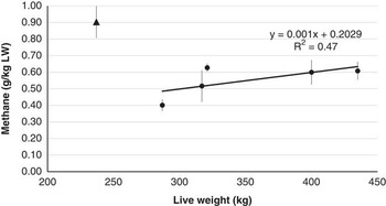
Growing cattle including steers and heifers were used for all deployments except Douglas Daly where mature cows were used. The mean BW of cattle across six deployments ranged from 237 to 435 kg, thus closely covering the BW range of cattle from post-weaning to maturity under extensive Australian conditions. When the Lansdown data were removed from the analysis, BW accounted for 47% of the variation in emissions per kg BW with a trend towards higher emissions in larger cattle (Figure 3). Even though Lansdown cattle were the lightest, their emissions per kg BW were contrary to the trend for other cattle, further casting doubt on the veracity of the Lansdown data. There was no discernible effect of sex, physiological state or breed on CH₄ emissions, although these studies were not designed explicitly to study these effects.

Figure 3

The relationship between BW of cattle and their methane emission (g/kg BW). The black triangle is the Lansdown data, black circles represent data from the other deployments.

Extensive grazing implies a dispersed emission of CH₄ from cattle over a large area. Under these conditions the CH₄ signal strength is too low for accurate estimation of emissions using current OPL technology. Use of tracer gases can be of value under these situations and have been used in open path-Fournier transformed infra-red (OP-FTIR) laser measurements (Phillips et al., Reference Phillips, McPhee, Hegarty and Naylor2013) but are impractical. On-animal tracer release devices can become dislodged and need regular servicing, the OP-FTIR requires a 240 V power source, the equipment is bulky and prone to damage in transit. As an alternative, we measured CH₄ emissions at a herd scale during a time of day when free-ranging cattle tend to congregate around an attractant, usually water (Tomkins et al., Reference Tomkins, McGinn, Turner and Charmley2009). It is well known that there are diurnal variations in CH₄ emissions, with peaks in CH₄ output following grazing bouts (Tomkins et al., Reference Todd, Altman, Cole and Waldrip2011; McGinn et al., Reference McGinn, Flesch, Coates, Charmley, Chen, Bai and Bishop-Hurley2015). Behavioural observations on cattle grazing under northern Australian conditions have demonstrated a crepuscular grazing pattern with a rest period during the hottest part of the day (Tomkins et al., Reference Tomkins, McGinn, Turner and Charmley2009). Thus, constraining cattle around a water point following morning grazing was considered to have the least impact on typical grazing behaviour. However, it was also expected that the measurement period would coincide with a peak in hourly emissions. Several reports where the OPL technique has been used to measure emissions over 24 h have demonstrated that emissions are 12% to 14% higher between 0800 and 1600 h compared with the rest of the 24-h period (McGinn et al., Reference McGinn, Turner, Tomkins, Charmley and Chen2011 and Reference McGinn, Flesch, Coates, Charmley, Chen, Bai and Bishop-Hurley2015; Tomkins et al., Reference Todd, Altman, Cole and Waldrip2011). Consequently, it can be assumed that the observed values in the current studies would be ~8% greater than the daily mean.

As noted earlier (Table 4) we concluded that our measured emissions over 5 to 7 h during the day appeared to be somewhat higher than expected when they were used to estimate DMI. By adjusting for the 8% diel effect, the average emissions across all six deployments inferred a DMI of ~25 g/kg BW (excluding Lansdown data).

CH₄ emissions variability within the day

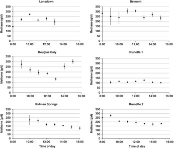
Figure 4 shows the mean hourly emission (multiplied by 24 to present a daily emission rate) for each site during the measurement period (~0800 to 1600 h). There was considerable variation in the hourly mean values within sites. For three of the deployments there was an ~50 g/day range in emissions due to sampling time (Lansdown, Belmont and the first Brunette Downs deployment). For those sites where the hourly range in emissions was high, being 100 to 150 g/day, this was generally attributed to emissions taken during the first 2 h of measurement being considerably higher than emissions taken later in the day. Several factors could have contributed to higher values in the early morning. These include generally lower wind speeds and therefore lower atmospheric stability or a requirement for the OPL to achieve a recommended operating temperature after having been turned off overnight to conserve battery power (McGinn S.M., personal communication). As standard practice OPL were powered up for 2 h before actual measurements but this was not always possible particularly at the more remote sites of Kidman Springs and Brunette Downs. Hourly variation in emissions are typical of data collected using OPL techniques. The method itself contributes to this as data filtering contributes to random missing values, thus influencing hourly mean values for each day. Using similar filtering methods to those employed in our study McGinn et al. (Reference McGinn, Flesch, Coates, Charmley, Chen, Bai and Bishop-Hurley2015) recorded 53% useable data, but the variation in useable data across their treatments ranged from a low of 19% to a maximum of 72% useable values.

Figure 4

Mean (±SE) hourly methane emissions during the measurement period for the six field campaigns.

CH₄ emissions are related to feeding bouts, with CH₄ peaks typically occurring within 2 h of feeding. Since cattle grazing extensive pastures in the tropics typically have major grazing bouts around dawn and dusk (Tomkins et al., Reference Tomkins, McGinn, Turner and Charmley2009) a post-prandial peak in CH₄ emissions is sometimes observed in OPL experiments. Tomkins et al. (Reference Todd, Altman, Cole and Waldrip2011) observed a significant peak between 1000 and 1700 h using OPL when cattle grazed a Rhodes grass pasture, but this peak was not apparent when the same pasture was cut and carried and fed in open circuit CH₄ chambers. McGinn et al. (Reference McGinn, Flesch, Coates, Charmley, Chen, Bai and Bishop-Hurley2015) observed a similar but much less pronounced pattern of CH₄ emissions. In the current deployments it was not possible to identify the expected post-prandial peak in emissions as observed by Tomkins et al. (Reference Todd, Altman, Cole and Waldrip2011) and McGinn et al. (Reference McGinn, Flesch, Coates, Charmley, Chen, Bai and Bishop-Hurley2015). Such peaks could be difficult to discern without the pre-prandial data for comparison. Patterns in emissions over the 7 to 8 h observation periods were variable and did not adhere to any biologically sensible relationship. These data, however, stress the importance of a suitably long sampling period over many days and at relatively high frequency. Increasing the number of observations reduces the importance of any single data point. While any individual data point will be subject to a range of events affecting the actual reading, by collecting many readings over the day or several days, we believe this method gives an accurate representation of the true emissions over time.

CH₄ emissions variability across deployments

As has been noted already, data obtained from the deployment on Lansdown Research Station was outside the expected range and are not considered in this section. Among the five successful deployments CH₄ emissions varied between 0.4 and 0.6 g/kg BW. Field-based measurements from grazing livestock using either SF₆ or a range of laser-based techniques corroborate our results. Boland et al. (Reference Boland, Quinlan, Pierce, Lynch, Kenny, Kelly and Purcell2013) using the SF₆ tracer gas technique recorded CH₄ emissions from dairy heifers grazing good quality temperate pastures of 0.35 to 0.4 g/kg BW. Similarly, Chaves et al. (Reference Chaves, Thompson, Iwaasa, Scott, Olson, Benchaar, Veira and McAllister2006) observed values of between 0.3 and 0.45 g/kg BW for grazing heifers in the Canadian prairies, while data from the United Kingdom for perennial ryegrass indicated higher emissions of 0.59 g/kg BW (Hammond et al., Reference Hammond, Humphries, Westbury, Thompson and Crompton2014). Data collected under tropical conditions using the OPL range between 0.52 and 0.56 g/kg BW (McGinn et al., Reference McGinn, Turner, Tomkins, Charmley and Chen2011; Tomkins et al., Reference Todd, Altman, Cole and Waldrip2011; McGinn et al., Reference McGinn, Flesch, Coates, Charmley, Chen, Bai and Bishop-Hurley2015).

This study was designed to obtain data from the major beef regions of northern Australia and the sites cover a wide diversity of soil, climate, management and livestock types. The variability in emissions across sites cannot be meaningfully ascribed to any particular site-specific variable but do suggest that across a wide range of conditions, CH₄ emissions are relatively consistent, particularly when compared with the variability in emissions from much more controlled experimental designs (Hammond et al., Reference Hammond, Humphries, Westbury, Thompson and Crompton2014; McGinn et al., Reference McGinn, Flesch, Coates, Charmley, Chen, Bai and Bishop-Hurley2015). However, Figure 3 suggests that there was a tendency for emissions per unit BW to increase as BW increased.

It is widely published that there is a relationship between diet digestibility and CH₄ emissions with emissions per unit intake decreasing with increasing diet digestibility (e.g. Benchaar et al., Reference Benchaar, Pomar and Chiquette2001; Yan et al., Reference Yan, Porter and Mayne2009; Hristov et al., Reference Holechek2013). However, DMI increases with increasing diet quality so the effect of diet quality on daily emissions is variable, depending on the magnitude of decreasing emissions (g/kg DMI) and increasing intake as diet quality increases. In the current study, pasture composition was recorded, but not actual diet quality due to the heterogeneous nature of the pastures. However, five of the six deployments occurred in the mid to late dry season of northern Australia. At this time of year forage quality is consistently poor with OM digestibility values between 0.45 to 0.55 and CP content <80 g/kg DM (Ash et al., 1997); conditions conducive to high emissions relative to intake. At Brunette Downs, there were two deployments with the same cattle at the beginning and end of the dry season and a contrast in diet quality was to be expected. CH₄ emissions were higher at the end of the dry season, a finding that is consistent with the expected poorer diet quality. However, caution should be exercised in linking diet quality to daily emissions when DMI is not known.

The direct measurement of enteric CH₄ emissions from livestock under extensive grazing systems is challenging. This paper demonstrates that the OPL technique is a satisfactory option, when employed on aggregations of grazing cattle for 7 to 8 h a day over 7 to 14 days. Logistical constraints limited the number of deployments, thus it was difficult to draw conclusions regarding factors that influenced the variation in emissions across deployments of between 0.4 and 0.63 g/kg BW (excluding data from one site). Effects of diet quality and BW of cattle may have been contributing factors but cannot be confirmed. The data presented in this paper are within the expected range for emissions from grazing cattle and suggest that this method is a viable option for directly measuring CH₄ emissions from cattle at the herd scale in extensive grazing conditions.