Nomenclature
-
 $a,b,{c_i},{d_i}$
-
model parameters
-
$A,B,{C_i}$
-
augmented model matrices
-
${A_e}$
-
exit area
-
${C_v}$
-
nozzle exit velocity coefficient
-
$EGT$
-
exhaust gas temperature
-
$FAR$
-
fuel to air ratio
-
$G$
-
transfer function
-
$h$
-
enthalpy
-
$H$
-
fuel heating value
-
$I$
-
identity matrix
- ISA
-
International Standard Atmosphere
-
$J$
-
moment of inertia of the rotor
-
$K$
-
percentage of pressure drop
-
${K_i}$
-
feedback gain i
-
$\dot m$
-
mass flow
-
$M$
-
Mach
-
$N$
-
spool speed
-
$\dot N$
-
spool acceleration
-
${N_c}$
-
corrected spool speed
-
${p_i}$
-
reference prefilter gain i
-
${P_{amb}}$
-
ambient pressure
-
${P_s}$
-
Sstatic pressure
-
${P_{std}}$
-
standard pressure
-
${P_{tin}}$
-
total inlet pressure
-
${P_{tout}}$
-
total outlet pressure
- PI
-
proportional integral controller
- PLA
-
power level angle
-
${r_i}$
-
setpoint i
- SLS
-
standard sea-level
-
${t_i}$
-
output of memory-less function i
-
${T_{std}}$
-
standard temperature
-
${T_{tin}}$
-
total inlet temperature
-
${T_{tout}}$
-
total outlet temperature
-
$u$
-
control input
-
${u_r}$
-
control input rate
-
$V$
-
Lyapunov function
-
${W_f}$
-
fuel flow
-
$x$
-
state variable
-
$X$
-
augmented state vector
-
${y_i}$
-
increment of the output i
-
${z_i}$
-
input of memory-less function i


Greek symbol
-
$\delta $
-
non-dimensional pressure
-
$\eta $
-
efficiency
-
$\theta $
-
non-dimensional temperature
-
$\Lambda $
-
vector containing static nonlinearities
-
$\pi $
-
pressure ratio
-
$\tau $
-
torque
-
${\Omega _i}$
-
diagonal matrix i for sector definition


1.0 Introduction
The application of small turbine engines for aircraft propulsion is remarkable. In this area, microjet engines are more preferred because of their straightforward design, fewer components, and lower cost. A significant challenge with these engines is the availability of limited sensors for control and condition monitoring. Typically, these engines are equipped with only two sensors: one for measuring engine speed, and another for exhaust gas temperature. On the other side, fuel flow is the sole variable used for managing thrust and operational limits. Despite these circumstances, these engines must exhibit efficient performance across a range of flight conditions, including varying Mach numbers and altitudes. To enhance the design and efficiency of small turbojet engines, numerous studies have been carried out focusing on modeling, performance analysis, and the development and implementation of control systems. In research conducted by Catana et al. [Reference Catana, Cican and Badea1], the primary parameters and performance assessment of microjet engines were examined during the take-off phase as well as under various operating conditions. The analysis was based on thermodynamic evaluations of several engines produced by various manufacturers, including JetCat and AMT Netherlands. The engines examined featured an identical spool design, yet they varied in thrust classes, with outputs ranging from 97 to 1569 N. In another study, Erario et al. [Reference Erario, De Giorgi and Przysowa2] created a numerical model of a micro gas turbine designed to predict and assess engine performance using the gas turbine simulation program (GSP). To evaluate the engine’s performance during bench and flight tests, they employed scaled maps of the compressor and turbine within a zero-dimensional model. The exhaust gas temperature (EGT) and fuel flow were selected as the primary parameters to validate the model by comparing the numerically predicted values with the experimental data. Gaitanis et al. [Reference Gaitanis, Contino and Paepe3] introduced a numerical tool created using the Python programming language, aimed at predicting the performance of micro gas turbines. The primary objective of their research was to attain a high level of accuracy in the simulated dynamic responses. A significant advantage of this tool lies in its uncomplicated component modules. They validated their model through experimental data obtained from the VUB T100 test rig. In another research [Reference Many, Weber, Oberndorfer, Koeberle, Hosseini and Hornung4], a parametric white-box model was developed to capture the transient dynamics of the JetCAT P100-RX turbojet engine using MATLAB/Simulink. In this investigation, scaling techniques were employed to adjust the component performance maps. A state-space representation of the engine was established, and critical parameters were determined through system identification methods. In a separate study [Reference Momin, Nava, L’Erario, Mohamed, Bergonti, Vanteddu, Braghin and Pucci5], researchers proposed a methodology for estimating online thrust for the small-scale turbojets utilised in aerial robots. They implemented a grey-box approach to model the dynamics of the turbojet system using a nonlinear state-space framework, informed by data collected from a specially designed engine test bench. This model subsequently facilitated the design of an extended Kalman filter, which estimates turbojet thrust based solely on angular speed measurements. In research by Metin and Aygun [Reference Metin and Aygün6], dynamic energetic and performance measures of a small turbojet engine were calculated at various shaft speeds. Then, based on the calculated parameters, efficiencies, power and energy indexes of the engine were extracted. In another study by Aygun et al. [Reference Aygun, Dursun, Dönmez, Sahin and Toraman7], thrust, exhaust gas temperature and specific fuel consumption of a micro turbojet engine (MTJ-E) were predicted by a machine learning technique and using the experimental data of fuel flow, air mass flow, exhaust gas velocity, compressor inlet and outlet pressures and turbine RPM.
Several studies have been published regarding the control of small turbojet engines. Banazadeh et al. [Reference Banazadeh, Gol and Ramazani8] employed an identification technique alongside frequency response test data to identify the transfer functions linking fuel flow to thrust, spool speed, compressor outlet pressure and turbine outlet temperature in a microturbine engine. Subsequently, they created a proportional integral derivative (PID) controller for the nonlinear system based on the models obtained. In a separate study, researchers introduced a modular control system for small gas turbine engines [Reference Andoga, Főző, Judičák, Bréda, Szabo, Rozenberg and Džunda9]. This control framework utilised situational control methodology and incorporated a diagnostic system as well. The controller was successfully implemented in a laboratory setting for the ISTC-21v and TJ-100 small turbojet engines. Beneda and Derbel [Reference Beneda and Derbel10] employed the turbofan power ratio, typically applied to high-bypass turbofan engines, to control a micro-turbojet engine. They developed a two-degree-of-freedom PID controller for the engine. In another research [Reference Derbel and Beneda11], they designed a sliding mode controller based on the turbofan power ratio. They modeled a small turbojet engine in the form of a linear parameter varying (LPV) structure and compared the performance of the proposed controller with a PID controller. Tang et al. [Reference Tang, Wang, Gu and Gu12] developed an adaptive PID controller based on neural networks for a micro-turbojet engine used in small unmanned aircraft. Their design allowed for real-time adjustment of the controller coefficients. While they applied their approach to control the engine spool speed, they did not consider the limitations associated with the engine’s variables. Shehata et al. [Reference Shehata, Khalil and Ashry13] provided a digital PID controller specifically for the JetCat-P200sx micro turbojet engine, employing an optimal control approach and a genetic algorithm to fine-tune the controller coefficients. They assessed the robustness of both methods by evaluating their effectiveness in noise and disturbance rejection. In a separate investigation, they utilised an adaptive fuzzy approach to modify the controller coefficients and examined the controller’s performance in relation to the engine model within the MATLAB-Simulink environment [Reference Shehata, Khalil and Ashry14]. Gao et al. [Reference Gao, Li and Zhang15] developed a PID controller to attain a stable control of engine speed during slow engine operating conditions. To optimise the tuning of the PID parameters, they proposed an enhanced evolutionary strategy for the self-adjustment of control variables within the engine speed and fuel flow management system. In another study [Reference Wang, Xu and Li16], researchers examined the active disturbance rejection control (ADRC) approach to improve the disturbance resistance of the control system for a small-scale turbojet engine. They established an ADRC scheme with spool speed as the controlled variable and evaluated its performance against a PID control method through simulation experiments.
In most of the control methods developed for small turbojet engines in the open literature, traditional control techniques are employed to manage engine thrust. However, these control systems typically do not incorporate critical engine constraints such as turbine temperature limits, compressor surge margin and combustor blow-out into their strategy. As a result, most of the proposed controllers lack the necessary depth and effectiveness for practical application. Therefore, utilising a decentralised architecture with multi-loop control systems for engine thrust control and limit management is more efficient than relying on a centralised structure. In this context, a Min-Max controller was developed for a turbojet engine by Jafari and Nikolaidis [Reference Jafari and Nikolaidis17]. To enhance the controller’s performance in terms of thrust tracking and response speed, fuzzy T and S norms were utilised instead of the conventional minimum and maximum functions. Their proposed scheme incorporated only proportional (P) controllers and did not take into account the turbine temperature limit. Furthermore, there was no strategy outlined for assessing the stability of the multi-loop system. Numerous studies [Reference Garg18–20] have explored the application of selector control schemes for managing large turbofan engines. Additionally, some research has introduced techniques to examine the stability of the control structure [Reference Richter21, Reference Imani and Montazeri-Gh22]. However, microjet engines are equipped with significantly fewer sensors and actuators compared to large turbofan engines, which complicates the tasks of controlling engine thrust and ensuring limit protection. To date, no thorough methodology has been presented that utilises a selective control structure along with a stability analysis procedure for small turbojet engines which only involve two measured variables and a single manipulated variable.
In this paper, a control algorithm is presented for control of small turbojet engines that only have two measured variables, and only one control input. In this algorithm, state feedback regulators are used to control the thrust and turbine temperature. Fuel flow rate saturation is also used to control the compressor surge and combustion chamber blow-out. Due to the presence of the minimum selector and the saturation function in the proposed algorithm, the issue of system stability is very important, and in this research, an efficient method for analysing the stability is presented. In order to assess the effectiveness of the developed controller, a simulation study is carried out employing a non-linear thermodynamic model of a small turbojet engine.
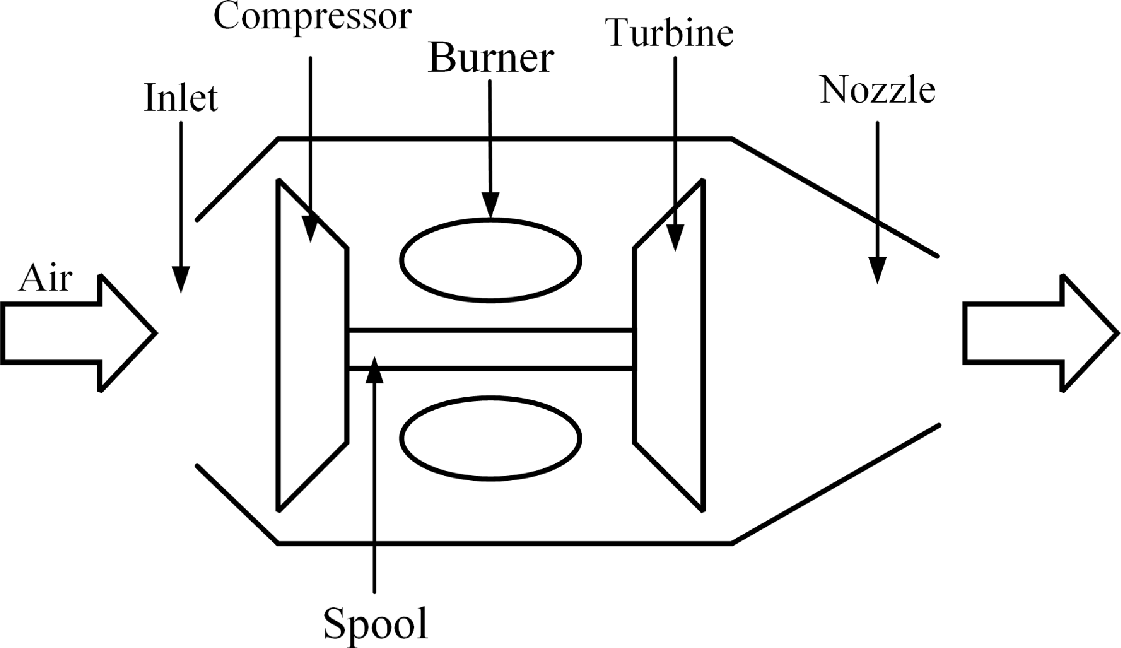
Schematic of the studied turbojet engine.

2.0 Thermodynamic modeling of the engine
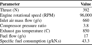
In the current research, the AMT NL Titan 40kg thrust engine is taken into account as a small-scale turbojet engine [23]. Figure 1 illustrates the primary structure of this engine, while its specifications are detailed in Table 1. The engine features a single-stage centrifugal compressor, an annular combustion chamber, and a single-stage axial turbine, and it is used as the propulsion system for some aerial vehicles such as the DEMON UAV [Reference Savvaris, Buonanno, Jamil and Tsourdos24].
Specifications of the studied engine [23]

The thermodynamic model of the engine developed in this study is based on a component-level framework. It is derived from the thermodynamic relations for the various engine components, including compressor, combustion chamber, turbine and nozzle. Additionally, it incorporates performance map data for the compressor and turbine [Reference Walsh and Fletcher25, Reference Lichtsinder and Levy26]. The average properties of the fluid at the input and output of each component are taken into account, and the scaled maps for the compressor and turbine are utilised. Engine modeling is conducted within the MATLAB-Simulink environment, and some of the capabilities of the toolbox for modeling and analysis of thermodynamic systems (T-MATS) offered by NASA Glenn Research Center (GRC) are utilised [Reference Zinnecker, Chapman, Lavelle and Litt27]. The relationships governing the engine components are described in the following subsections.
2.1 Compressor
Turbine engines are equipped with a compressor that increases the pressure of the incoming air before it reaches the combustor. The algebraic equations governing the compressor are described as follows [Reference Chung, Prasad, Dhingra and Meisner28]:
 \begin{align} \theta & = \frac{{{T_{tin}}}}{{{T_{std}}}},\,\,\,\delta = \frac{{{P_{tin}}}}{{{P_{std}}}},\,\,\,{N_c} = \frac{N}{{\sqrt \theta }}\nonumber\\[4pt]{{\dot m}_{c,map}} & = {f_1}\left( {{N_c},\beta line} \right)\nonumber\\[4pt]\pi & = {f_2}\left( {{N_c},\beta line} \right)\nonumber\\[4pt]\eta & = {f_3}\left( {{N_c},\beta line} \right)\nonumber\\[4pt]{{\dot m}_{out}} & = \frac{{{{\dot m}_{c,map}}}}{{{{\sqrt \theta } \mathord{\left/ {\vphantom {{\sqrt \theta } \delta }} \right. } \delta }}}\nonumber\\[4pt]{h_{tout}} & = \frac{{{h_{tout,ideal}} - {h_{tin}}}}{\eta } + {h_{tin}}\nonumber\\[2pt]{P_{tout}} & = \pi \left( {{P_{tin}}} \right),\,\,\,{T_{tout}} = f\left( {{P_{tout}},{h_{tout}}} \right)\nonumber\\[2pt]\tau & = \frac{{{{\dot m}_{out}}\left( {{h_{tin}} - {h_{tout}}} \right)}}{{N\left( {\frac{{2\pi }}{{60}}} \right)}}\end{align}
where
 ${f_1}$
,
 ${f_2}$
and
 ${f_3}$
are functions or lookup tables that represent the compressor map. Gas properties such as enthalpy and temperature are determined using gas tables.
2.2 Combustion chamber
In the combustion chamber, injected fuel is combined with compressed air and after combustion, high temperature gas is produced. The hot gas drives the turbine and create thrust as it passes through the nozzle. The pressure drop in the combustion chamber is assumed to be constant. The relationships related to this component are expressed as follows:
 \begin{align} {P_{tout}} & = \left( {1 - K} \right){P_{tin}}\nonumber\\[3pt]{{\dot m}_{gas,out}} & = {{\dot m}_{air,in}} + {{\dot m}_f}\nonumber\\[4pt]{h_{tout}} & = \frac{{{\eta _b}{{\dot m}_f}H + {{\dot m}_{in}}{h_{tin}}}}{{{{\dot m}_{out}}}}\nonumber\\[4pt]FAR & = \frac{{{{\dot m}_f}}}{{{{\dot m}_{air,in}}}}\end{align}
where K = 0.05 is the percentage of pressure drop in the combustor and H is the heating value of the fuel.
2.3 Turbine
Gas expansion in the turbine generates work of the rotor and drives the compressor. The turbine processes can be represented as follows:
 \begin{align} \theta & = \frac{{{T_{tin}}}}{{{T_{std}}}},\,\,\,\delta = \frac{{{P_{tin}}}}{{{P_{std}}}},\,\,\,{N_c} = \frac{N}{{\sqrt \theta }}\nonumber\\[4pt]{{\dot m}_{out}} & = {g_1}\left( {{N_c},\beta line} \right)\nonumber\\[3pt]\pi & = {g_2}\left( {{N_c},\beta line} \right)\nonumber\\[3pt]\eta & = {g_3}\left( {{N_c},\beta line} \right)\nonumber\\[3pt]{h_{tout\_g}} & = {h_{tin}} - ({h_{tin}} - {h_{tout\_g,ideal}})\eta \nonumber\\[3pt]{P_{tout}} & = \pi \left( {{P_{tin}}} \right),\,\,\,{T_{tout}} = f\left( {{P_{tout}},{h_{tout}}} \right)\nonumber\\[3pt]{h_{tout}} & = \frac{1}{{{{\dot m}_{out}}}}\left[ {{h_{tin}}{{\dot m}_{tin}} + \eta ({h_{tin}} - {h_{tout\_g,ideal}}){{\dot m}_{in}}} \right]\nonumber\\[5pt]\tau & = \frac{{{{\dot m}_{out}}({h_{tin}} - {h_{tout\_g}})}}{{N\left( {\frac{{2\pi }}{{60}}} \right)}} \end{align}
similar to the compressor,
 ${g_1}$
,
 ${g_2}$
and
 ${g_3}$
are a set of functions or lookup tables that define the turbine map.
2.4 Nozzle
The engine nozzle has a constant outlet area and is a converging type. In addition to the characteristics of the fluid entering the nozzle, the ambient static pressure at the nozzle exit affects the nozzle flow. Flow characteristics according to choking and non-choking conditions of the flow are specified by comparing the nozzle pressure ratio to the critical pressure.
 \begin{align} & \pi = \dfrac{{{P_{tin}}}}{{{P_{amb}}}}\nonumber\\[4pt]& {P_s} = g({h_{tin}},{P_{tout}},M = 1)\nonumber\\[3pt]& {\pi _{critical}} = \dfrac{{{P_{tin}}}}{{{P_s}}}\nonumber\\[3pt]& {\rm{If \, }}\pi \gt {\pi _{critical}}\nonumber\\[3pt]& \left[ {{P_s},u} \right] = {g_1}({h_{tin}},{P_{tout}},M = 1)\nonumber\\[3pt]& {\rm{else}}\nonumber\\[3pt]& \left[ {{P_s},u} \right] = {g_2}({h_{tin}},{P_{tout}},{P_s} = {P_{amb}})\nonumber\\[3pt]& Thrust = {{\dot m}_{out}}u{C_v} + ({P_{out}} - {P_{amb}}){A_e},\,\,\,{C_v} = 1 \end{align}
2.5 Shaft
Using the torque supplied by the turbine and the torque used by the compressor, the shaft dynamics can be written as follows:
 \begin{align} \dot N = \dfrac{{\Delta \tau }}{{J\left( {\dfrac{{2\pi }}{{60}}} \right)}} \end{align}
where
 $\dot N$
is the shaft angular acceleration,
 $\Delta \tau $
represents the difference between the torque generated by the turbine and the torque demanded by the compressor, and J is the moment of inertia of the rotor. In order to obtain the thermodynamic model by matrix iteration technique, a number of engine parameters are guessed and the same number of errors are defined. For this objective, in this study, inlet air mass flow, beta values for the compressor and turbine are estimated and the errors related to mass conservation in the compressor, turbine and nozzle are considered. The guesses are updated at each iteration through a numerical procedure until the errors are less than a pre-defined value. The numerical process is generally performed using the iterative Newton–Raphson procedure [Reference Walsh and Fletcher25]. Figure 2 shows the iterative process of solving the equations to achieve the transient model.
Iterative procedure for engine thermodynamic modeling.

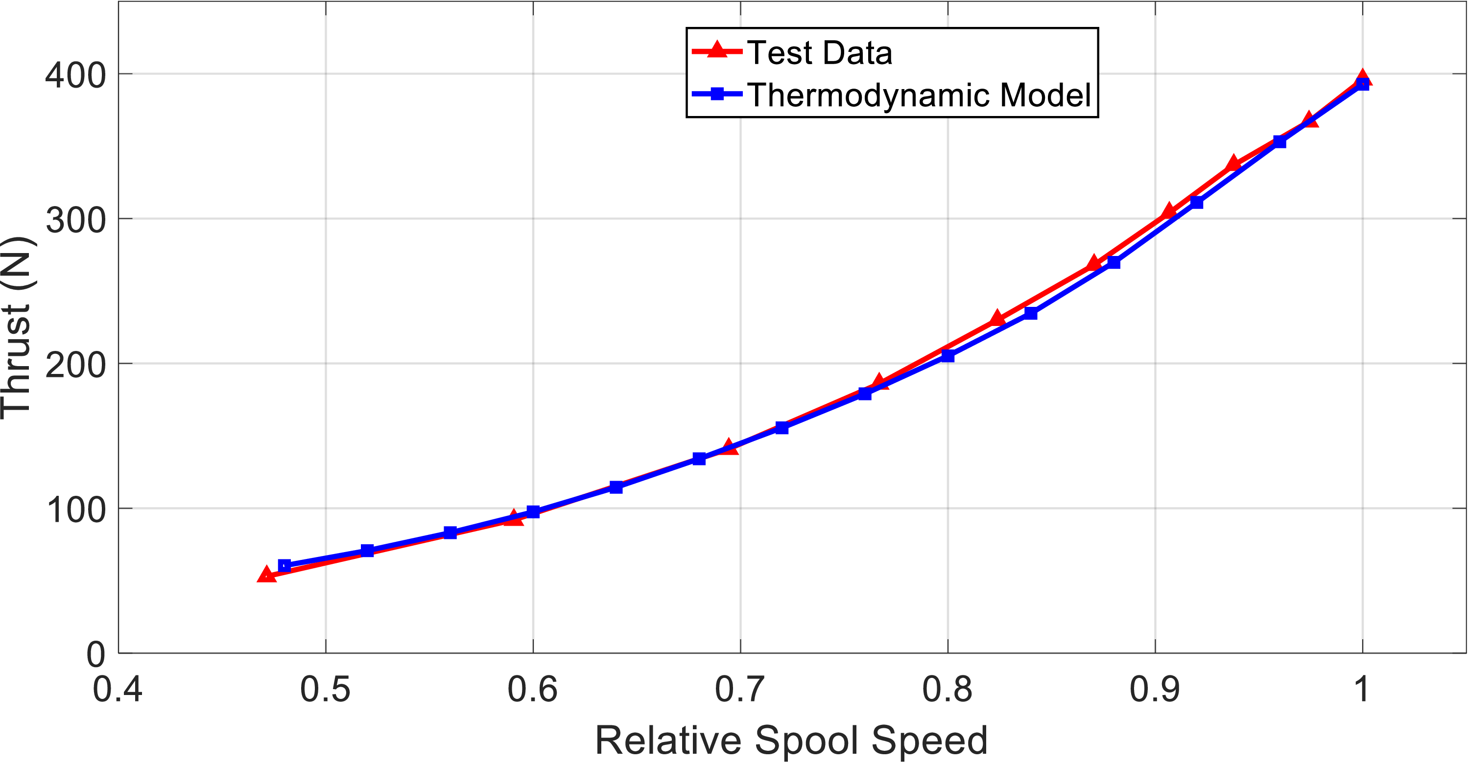
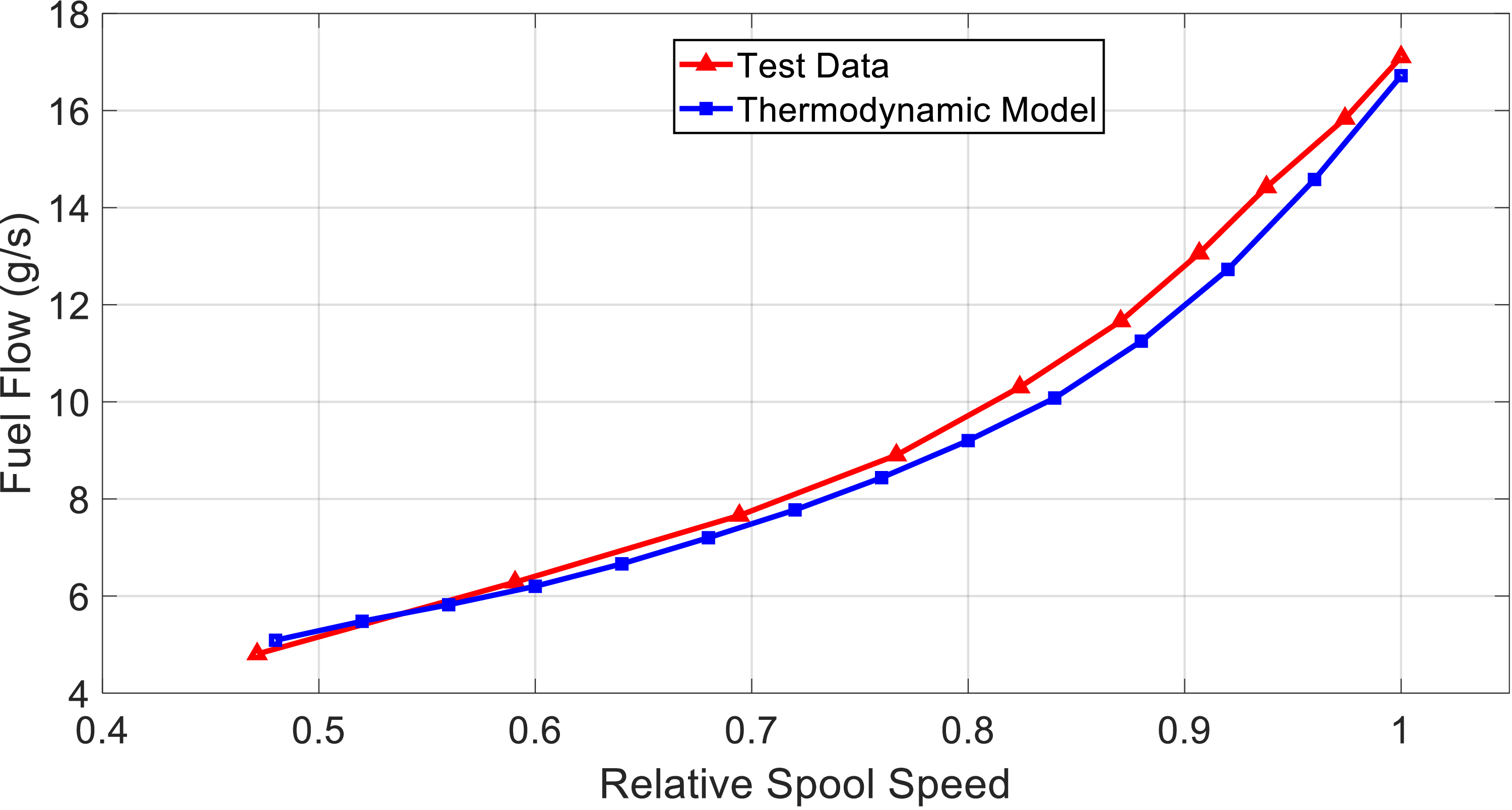
In order to show the validity of the modeling, according to Figs. 3 and 4, two important outputs of the engine (i.e., the thrust value and fuel flow) in terms of relative spool speed, have been compared with the engine test data. The maximum mismatch error for thrust is 3%, and for fuel consumption is 6%. Therefore, the obtained thermodynamic model has sufficient validity for performance analysis and controller design.
Engine thrust versus relative spool speed.

Engine fuel flow versus relative spool speed.

Because there is no explicit nonlinear dynamic equation for gas turbine engines, the nonlinear thermodynamic model is linearised around an operating point through identification techniques for the purpose of controller design. The linear model of the system with integrated input is expressed as
 \begin{align} \begin{array}{l}\dot x = ax + bu\\\dot u = {u_r}\\{y_i} = {c_i}x + {d_i}u\end{array} \end{align}
where
 $x = \Delta N$
is the state variable (i.e., engine speed increment) in rpm,
 $u = \Delta {W_f}$
is the control input (i.e., fuel flow increment) in kilograms per second (kg/s), and
 ${y_i}$
are increments of the outputs.
3.0 Control strategy
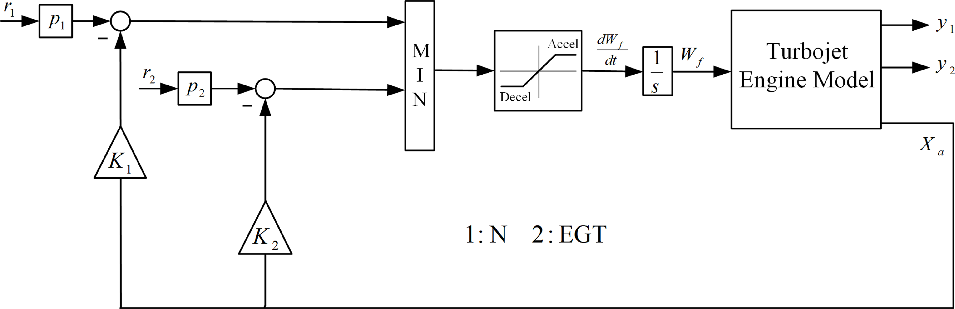
The engine controller must provide the desired thrust and at the same time protect the limits of turbine temperature, maximum engine speed, compressor surge and combustion chamber blow-out. To achieve this objective, a selective control strategy [Reference Cai, Wang, Chen, Zheng and Zhang29, Reference Eslami and Banazadeh30] has been taken into account. The structure of the proposed controller is illustrated in Fig. 5. Considering that engine thrust cannot be measured in flight conditions [Reference Singh, Maity and Nataraj31], therefore, a control loop is considered for engine spool speed as thrust representative. The relationship between thrust and engine speed is non-linear, and based on a lookup table, the thrust command is converted to its equivalent spool speed. This control loop should be designed in such a way that the response of the controller is without overshoot so that while providing the desired speed command, the engine speed does not exceed the maximum allowed value. As the engine speed increases, it’s crucial that the temperature of the turbine remains within the acceptable range to prevent damage to the turbine blades. Measuring the turbine inlet temperature (TIT) directly is challenging due to its extreme heat. Consequently, to avoid exceeding TIT limit, it is managed indirectly through the regulation of the engine EGT. Therefore, an EGT control loop is included in the controller structure and its output is compared with the output of the previous loop and the minimum value is selected. A significant challenge in engine control is the prevention of the dangerous compressor surge phenomenon. Since the risk of compressor surge increases during the engine’s rapid acceleration, restricting the engine’s acceleration can greatly minimise the probability of this occurrence. Limiting the acceleration of the engine can be achieved by limiting the fuel flow rate, therefore, by considering the output of the speed control loop and the EGT control loop as the fuel flow rate, and by using the upper saturation limit for the fuel flow rate, it is possible to prevent rapid acceleration and compressor surge [Reference DeCastro, Litt and Frederick32, Reference Litt, Frederick and Guo33]. Another important challenge of the engine is the possibility of lean blow-out in the conditions of instantaneous throttle reduction. When the throttle is reduced abruptly, the fuel supplied by the power level angle (PLA) control loop is also immediately decreased. This leads to a significant drop in the fuel-to-air ratio and raises the risk of combustion chamber blow-out. To reduce this risk, the engine’s deceleration is controlled. In this circumstance, a lower saturation limit for the fuel flow rate is considered to prevent the instantaneous reduction of the fuel flow and the combustion chamber blow-out. The output of the saturation function after passing through an integrator determines the amount of engine fuel. State feedback regulators are used to control engine speed and EGT temperature in the proposed controller structure.
The structure of the proposed controller.

In summary, it can be stated that the engine controller is responsible for meeting the required spool speed demand, which represents the thrust value, while also ensuring that the following variables remain within their limits during both steady-state and transient conditions:
 \begin{align} \left\{ \begin{array}{l}\Delta EGT\left( {{y_2} \le {r_2}} \right)\\[9pt]\dfrac{{d{W_f}}}{{dt}}\left( {{u_{r\min }} \le {u_r} \le {u_{r\max }}} \right)\end{array} \right. \end{align}
To formulate state feedback regulators, the linear system (1) can be expressed in the following augmented representation:
 \begin{align} \begin{array}{*{20}{c}}{\begin{array}{*{20}{c}}{\dot X = AX + B{u_r}} \quad {}{{y_i} = {C_i}X}\end{array}}\\[9pt]{\begin{array}{*{20}{c}}{A = \left[ {\begin{array}{*{20}{c}}a \quad {}b\\0 \quad {}0\end{array}} \right]} {}{\begin{array}{*{20}{c}}{B = \left[ {\begin{array}{*{20}{c}}0\\1\end{array}} \right]} {}{{C_i} = \left[ {\begin{array}{*{20}{c}}{{c_i}} \quad {}{{d_i}}\end{array}} \right]}\end{array}}\end{array}}\end{array} \end{align}
where
 $X = {\left[ {\begin{array}{*{20}{c}}x \quad {}u\end{array}} \right]^T}$
is the augmented state vector. State feedback control law for each individual control loop is regarded as follows:
 \begin{align} {u_{ri}} = - {K_i}X + {p_i}{r_i} \end{align}
where feedback gain
 ${K_i}$
is established employing state feedback methods to ensure that
 $A - B{K_i}$
remains stable, while each control loop exhibits satisfactory performance without any overshoot. The constant parameters of
 ${r_i}$
, for
 $i = 1,2$
consist of the setpoint for the main output and the limit value for the restricted output, both of which are determined based on the reference command and the characteristics of the system. The
 ${p_i}$
gains are constant reference prefilter gains aimed at ensuring that
 ${y_i} = {C_i}X = {r_i}$
in steady-state condition. They are established based on the following relationship.
 \begin{align} {p_i} = {[ - C{(A - B{K_i})^{ - 1}}B]^{ - 1}} \end{align}
The following section presents a methodology for analysing the stability of the proposed control system.
4.0 Stability investigation
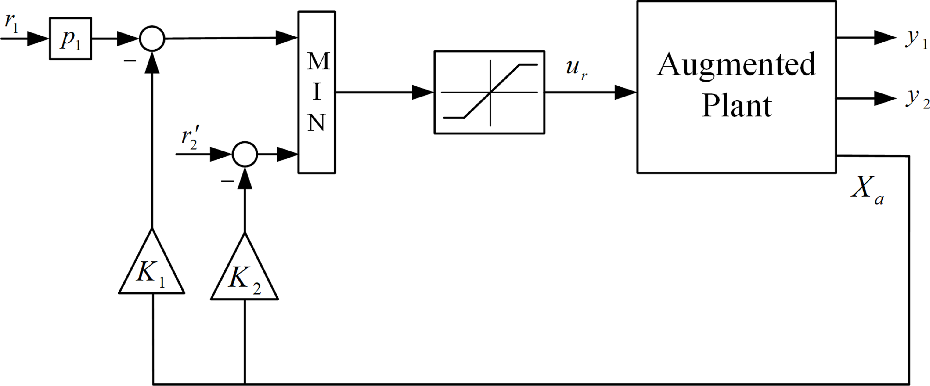
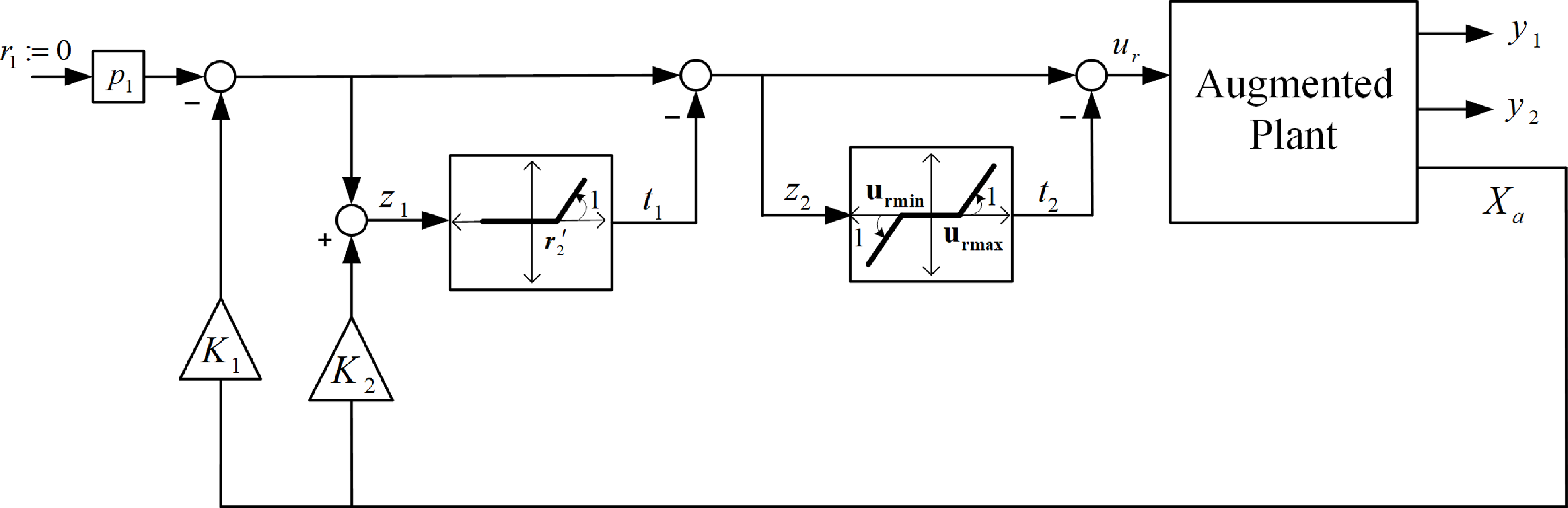
To investigate the stability of the designed controller depicted in Fig. 5, the controller’s architecture is converted into the standard configuration of Lure’s system [Reference Khalil34]. To achieve this, the initial step involves reconfiguring the plant, as illustrated in Fig. 6, resulting in its transformation into an augmented form. In the new configuration,
 ${r'_2} = {r_2}{p_2}$
. After that, according to Fig. 7, the Min selector and saturation function are replaced with their nonlinear equivalents [Reference Imani and Montazeri-Gh35]. In order to use the techniques of Lure’s problem [Reference Khalil34], the dynamics between the outputs
 ${t_i}$
and inputs
 ${z_i}$
of the nonlinear memory-less functions are extracted. Hence, using Fig. 7, we have
 \begin{align} \left\{ \begin{array}{l}{z_1} = - {K_1}X + {K_2}X = ({K_2} - {K_1})X\\[4pt]{z_2} = - {K_1}X - {t_1}\end{array} \right. \end{align}
Reconfiguration of the controller.

New depiction of the controller.

The relationship between
 $X = [x\ \ u]^T$
and
 ${u_r}$
can be determined from the transfer functions of the augmented plant, which is expressed as follows:
 \begin{align} G(s) = {[\begin{array}{*{20}{c}}{{G_1}(s)} \quad {{G_2}(s)}\end{array}]^T} = {\left[\begin{array}{*{20}{c}}{\dfrac{{x(s)}}{{{u_r}(s)}}} \quad {}{\dfrac{{u(s)}}{{{u_r}(s)}}}\end{array}\right]^T} \end{align}
control input rate is established from Fig. 7 based on the following equation:
 \begin{align} {u_r} = - {K_1}X - {t_1} - {t_2} \end{align}
by applying Equations (12) and (13),
 $X = [x\ \ u]^T$
and
 ${u_r}$
are derived according to the values of
 ${t_i}$
. Substituting
 $X$
into Equation (11) reveals the relationship between
 ${t_i}$
and
 ${z_i}$
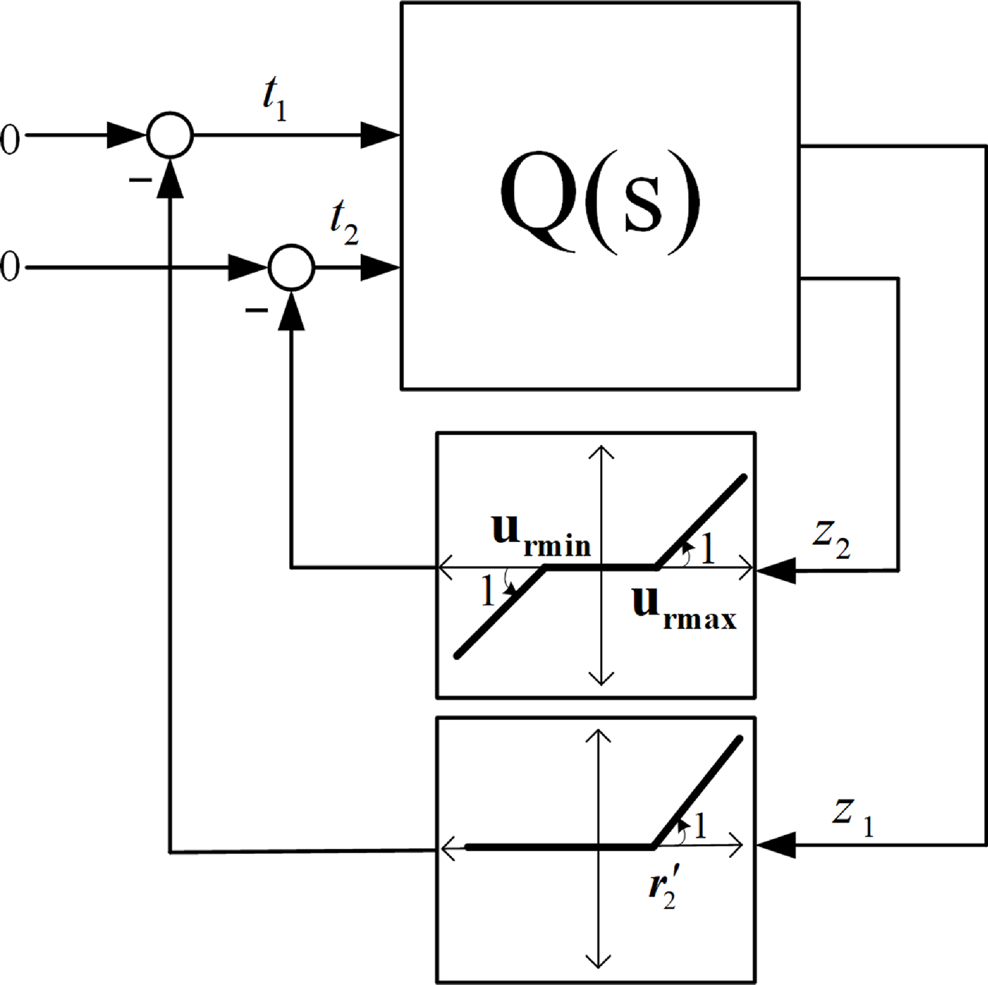
. Consequently, the control system illustrated in Fig. 7 can be represented as shown in Fig. 8, where matrix Q(s) expresses the dynamic relationship,
 \begin{align} Q(s) = \frac{{\left[ {\begin{array}{c@{\quad}c}{({K_2} - {K_1})G} & {}{({K_2} - {K_1})G}\\[4pt]1 & {}{ - {K_1}G}\end{array}} \right]}}{{{K_1}G + 1}} \end{align}
Closed-loop system arranged in a standard configuration.

 ${K_i}$
are state feedback gains and G is the vector of transfer functions (12).
The updated configuration, referred to as Lure’s system, incorporates a dynamic multivariate block along with static nonlinearities in the feedback loop. Based on the multivariate circle criterion [Reference Khalil34], if Q(s) represents a square and proper transfer function matrix with the following minimal realisation,
 \begin{align} \left\{ {\begin{array}{*{20}{c}}{\dot X = \hat AX + \hat BT}\\[5pt]{Z = \hat CX + \hat DT}\end{array}} \right. \end{align}
where
 $T = - \Lambda (Z)$
, and
 $\Lambda ( \! \cdot \! )$
is a vector containing static nonlinearities which are locally Lipschitz in Z and this vector satisfies the sector condition defined by real diagonal matrices
 ${\Omega _1}$
and
 ${\Omega _2}$
(i.e.,
 ${\left[ {\Lambda (Z) - {\Omega _1}Z} \right]^T}\left[ {\Lambda (Z) - {\Omega _2}Z} \right] \le 0$
), then the closed-loop system is globally asymptotically stable (or absolutely stable) around the equilibrium point
 $X = 0$
, if
 $[I + {\Omega _2}Q]{[I + {\Omega _1}Q]^{ - 1}}$
is strictly positive real. According to the static non-linear functions depicted in Fig. 8, matrix
 ${\Omega _1}$
is defined as a zero matrix. Consequently, to ensure asymptotic stability, it suffices for matrix
 $[I + {\Omega _2}Q]$
to be strictly positive real. To check the strictly positive real condition, the following lemma is taken into account [Reference Haddad and Bernstien36]:
Lemma [Reference Haddad and Bernstien36]: Let N(s) be a transfer function matrix with minimal realisation matrices
 $(E,F,H,J)$
, then the following statements are equivalent:
-
(1) E is a Hurwitz matrix and N(s) is strongly positive real
-
(2)
$J + {J^T} \gt 0$
and there exist positive definite matrices P and R such that
\begin{align*} {E^T}P + PE + {(H - {F^T}P)^T}{(J + {J^T})^{ - 1}}(H - {F^T}P) + R = 0 \\[-25pt]\end{align*}
It’s important to emphasise that strongly positive real implies strictly positive real [Reference Haddad and Bernstien36].


Utilising the minimum realisation of Q(s), we find that the minimal realisation matrices of
 $[I + {\Omega _2}Q]$
are
 $(\hat A,\hat B,{\Omega _2}\hat C,I + {\Omega _2}\hat D)$
. Now, according to the lemma statements, if matrix
 $\hat A$
is Hurwitz and
 $2I + {\Omega _2}\hat D + {\hat D^T}{\Omega _2}$
is positive definite, and if there exist positive definite matrices P and R such that fulfill the Riccati Equation (16), then
 $[I + {\Omega _2}Q]$
is strictly positive real and the multivariate circle condition is satisfied:
 \begin{align} {\hat A^T}P + P\hat A + {[{\Omega _2}\hat C - {\hat B^T}P]^T}{[2I + {\Omega _2}\hat D + {\hat D^T}{\Omega _2}]^{ - 1}}[{\Omega _2}\hat C - {\hat B^T}P] + R = 0 \end{align}
Consequently, the control system’s asymptotic stability around the origin
 $X = 0$
is assured, and
 $V = {X^T}PX$
is derived as a Lyapunov function for the closed-loop system [Reference Haddad and Bernstien36]. The asymptotic stability of the designed controller is investigated in the following section.
5.0 Results and discussion
To design the controller, assess its stability, and evaluate its performance, the nonlinear model has been linearised around an operating point (altitude = 0, Mach = 0 and
 ${W_f} = 15.5g/s$
). The parameters of the linear model include:
 \begin{align} a & = - 2.034, {}\quad b = 3.337 \times {{10}^6}\nonumber\\[5pt]\Delta N \, : \, c & = \left[ 1 \quad {}0 \right], {}\quad {d = 0}\nonumber\\[5pt]\Delta EGT \, : \, c & = \left[ 0.02153 {} \quad 0 \right],\quad {}d = 0\end{align}
Linear model (6) with the aforementioned parameters is both controllable and observable. State feedback regulators for the engine speed control loop and EGT are designed using pole placement technique. Each loop’s regulator is designed to ensure that the isolated loop remains stable while providing satisfactory performance. Consequently, the control gains are determined as follows:
 \begin{align} {K_1} & = \left[5.691e - 7 \quad {}4.966 \right],\nonumber\\[5pt]{K_2} & = \left[ 2.047e - 7 {} \quad 3.966 \right] \end{align}
prefilter gains
 ${p_i}$
are also obtained from Equation (10). The limit values of the restricted variables for linear system are taken into account as follows:
 \begin{align} {{r_2} = 115K,} {}{{u_{r\max }} = 0.02kg/{s^2},} \quad {}{{u_{r\min }} = - 0.02kg/{s^2}}\end{align}
For the stability analysis of the closed-loop system, the transfer function vector G is determined as:
 \begin{align} G(s) = {\left[ {\begin{array}{*{20}{c}}{\dfrac{{3.337e6}}{{{s^2} + 2.034s}}} \quad {}{\dfrac{1}{s}}\end{array}} \right]^T} \end{align}
The equivalent linear system Q(s) is defined in accordance with Equation (16) as follows:
 \begin{align} Q(s) = \frac{{\left[ {\begin{array}{c@{\quad}c}{ - {\rm{s }} - {\rm{3}}{\rm{.25}}} & {}{ - {\rm{s}} - {\rm{3}}{\rm{.25}}}\\[3pt]{{s^2} + 2.034s}& { - {\rm{4}}{\rm{.966 s }} - {\rm{12}}}\end{array}} \right]}}{{{s^2} + 7s + 12}} \end{align}
A minimal state space realisation of Q(s) is determined:
 \begin{align*} \hat A = \left[ \begin{array}{c@{\quad}c} - 3.3853 & 7.0337\\[2pt]00337 & - 3.6147\end{array} \right]\\[4pt]\hat B = \left[ \begin{array}{c@{\quad}c} - 0.9583 & - 0.9583\\[2pt]1.1419 & 1.1419\end{array} \right]\end{align*}
 \begin{align}\hat C & = \left[ \begin{array}{c@{\quad}c}0.0138 & - 0.8642\\[2pt]0.6001 & - 3.8454\end{array} \right]\nonumber\\[4pt]\hat D & = \left[ {\begin{array}{c@{\quad}c}0 {}& 0\\[2pt]1 {} & 0\end{array}} \right] \end{align}
The matrices
 ${\Omega _1}$
and
 ${\Omega _2}$
, which define the sectors, are established as follows:
The limits of the limited variables in nonlinear simulation

 \begin{align} \begin{array}{*{20}{c}}{{\Omega _1} = 0 \times {I_2},} \quad{{\Omega _2} = 0.97 \times {I_2}}\end{array} \end{align}
where
 ${I_2}$
is the
 $2 \times 2$
identity matrix. Based on the conditions obtained for the stability analysis,
 $\hat A$
is Hurwitz and
 $2I + {\Omega _2}\hat D + {\hat D^T}{\Omega _2}$
is positive definite. The Riccati Equation (6) can be formulated as a Linear Matrix Inequality (LMI) feasibility problem by utilising the Schur complement lemma [Reference Geromel37]. Therefore, the positive definite matrix P needs to satisfy the following inequality:
 \begin{align} \left[ {\begin{array}{*{20}{c}}{{{\hat A}^T}P + P\hat A} \quad {}{P\hat B - {{\hat C}^T}{\Omega _2}}\\[3pt]{{{\hat B}^T}P - {\Omega _2}\hat C} {} \quad { - 2I - {\Omega _2}\hat D - {{\hat D}^T}{\Omega _2}}\end{array}} \right] \lt 0 \end{align}
By addressing this feasibility problem, a positive definite matrix P is derived as follows:
 \begin{align} P = \left[ \begin{array}{c@{\quad}c} 0.3253 & - 0.7470\\[3pt] - 0.7470 & 2.8457\end{array} \right] \end{align}
Consequently, the asymptotic stability of the control system around
 $X = 0$
is assured, and the Lyapunov function
 $V = {X^T}PX$
for the closed-loop system is established.
To assess the effectiveness of the proposed control structure, its performance is compared to a PI controller. The PI controller controls the engine spool speed as thrust representative, and has been developed based on the spool speed transfer function at the specified operating point. This controller has an efficient manner in tracking the desired input. For instance, its response to the step command is almost overshoot-free (overshoot is less than 0.4%) and its rise time is 0.87 s. The gains of the designed PI controller are:
 \begin{align} \begin{array}{*{20}{c}}{{K_p} = 6.3 \times {{10}^{ - 7}},} \quad {}{{K_i} = 1.5 \times {{10}^{ - 6}}}\end{array} \end{align}
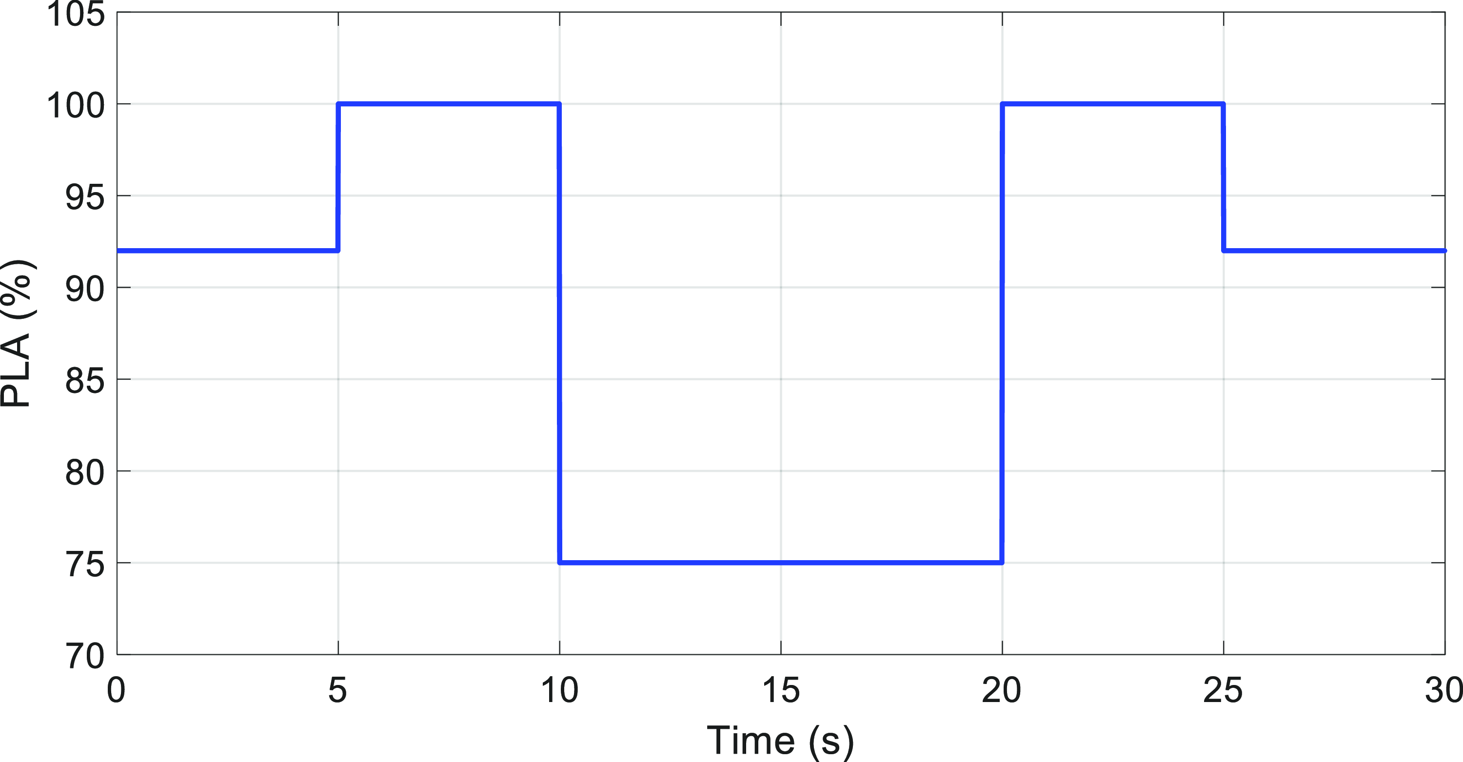
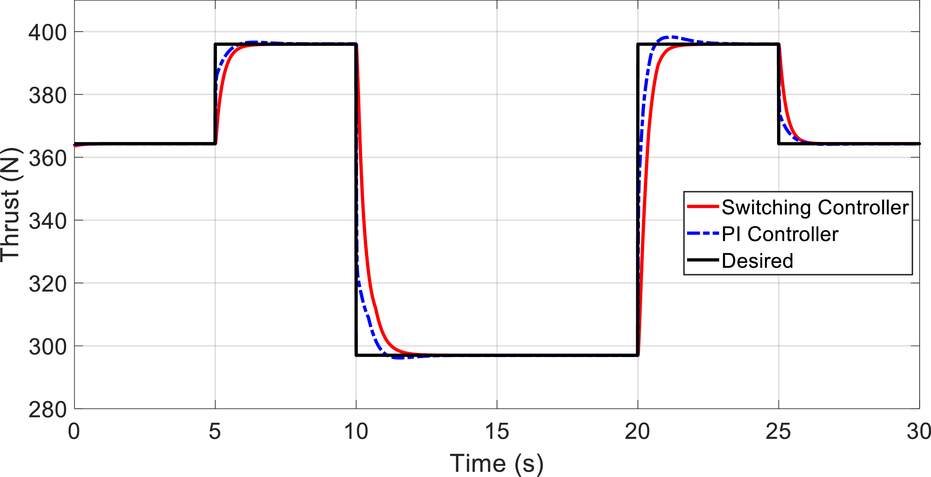
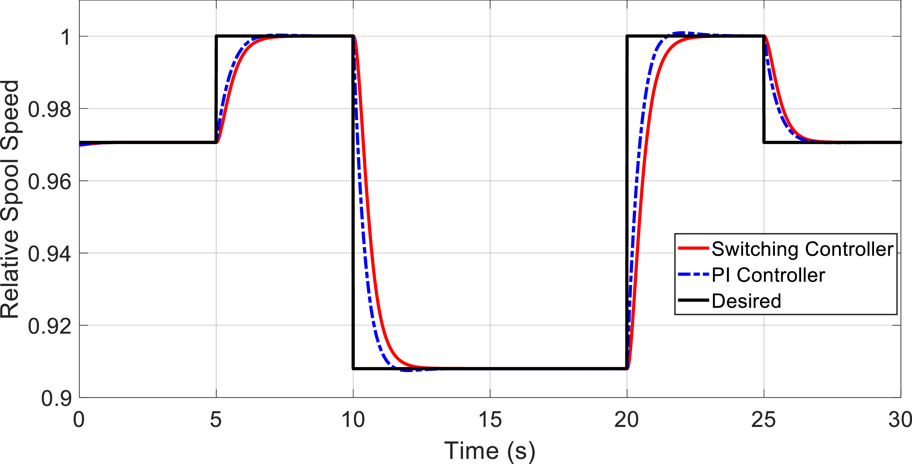
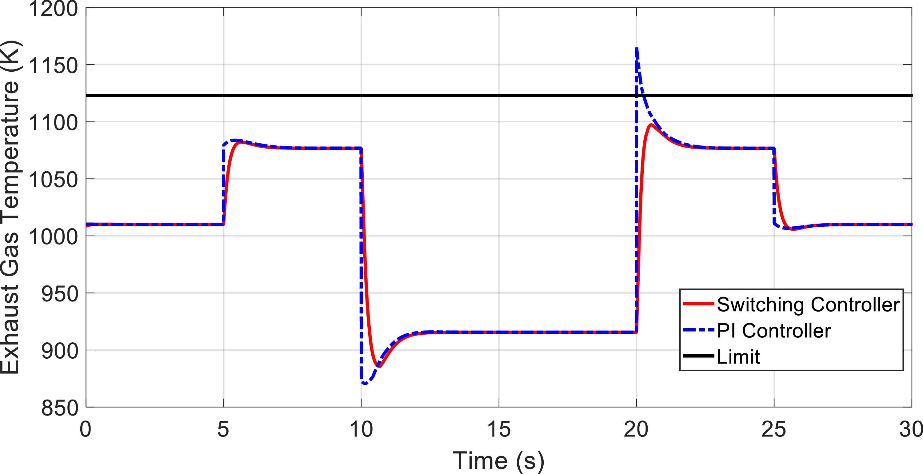
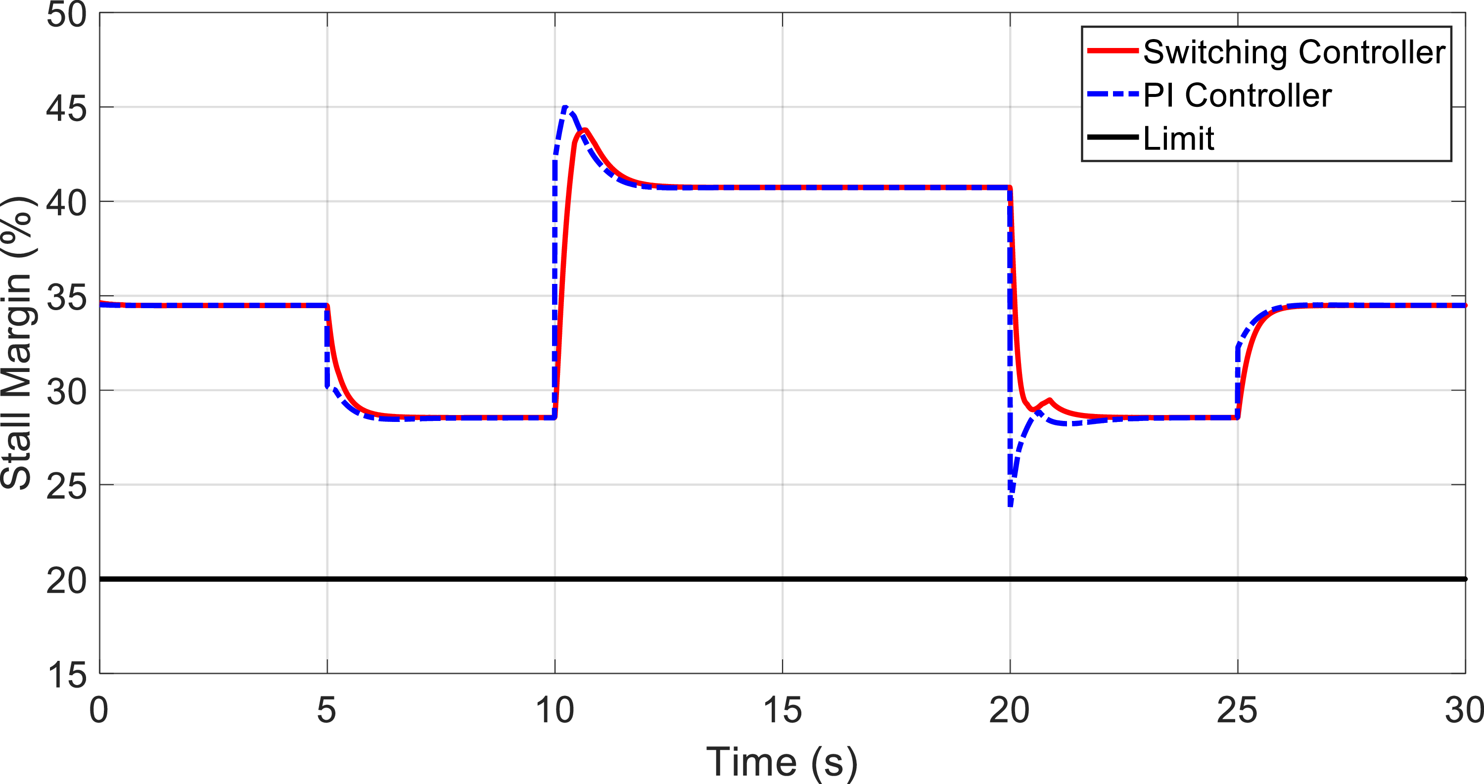
The limit values of the constrained variables for nonlinear simulation are presented in Table 2. The PLA degree is proportional to the thrust value, but it has a non-linear relationship with spool speed. As shown in Fig. 9, a comprehensive command for the PLA degree around the operating point is defined in the International Standard Atmosphere (ISA) and zero Mach and standard sea level (SLS) altitude conditions. PLA degree starts from 92% and varies between 75% and 100%. The system response is not necessarily satisfactory for simulation at lower PLA degree as well as at other Mach numbers and altitudes. Figure 10 shows the response of the controllers in tracking the desired thrust. The response of the PI controller is faster than the selector controller, but it has overshoot and undershoot in some places. As mentioned before, considering that the thrust value cannot be measured in flight conditions, this parameter is indirectly controlled through the engine speed. In Fig. 11, the process of following the desired spool speed using two controllers is shown. The response speed of the PI controller is slightly higher than that of the switching controller, but in some places, this controller has a limited overshoot and undershoot. Figure 12 illustrates the variations in the engine exhaust gas temperature for both controllers. The PI controller significantly surpasses the specified limit. This is because the PI controller just controls engine speed as the thrust representative it does not have any feedback from the limit violation of other engine outputs. Consequently, its efficacy in safeguarding the EGT limit is unacceptable. In Fig. 13, the surge margin of the compressor is indicated for both controllers. According to this figure, due to the presence of fuel flow rate saturation in the structure of the selector controller, this controller has a higher surge margin.
Throttle command.

Engine thrust response.

Spool speed response.

Exit gas temperature response.

Surge margin.

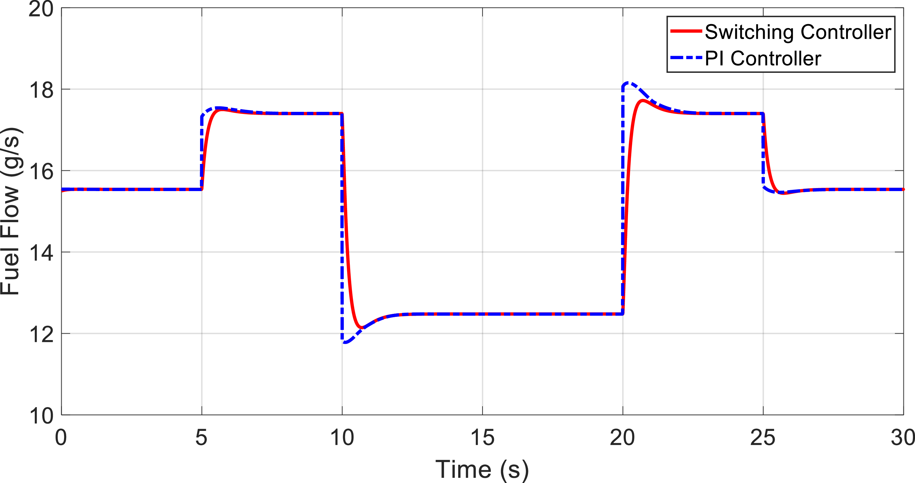
Fuel consumption.

Figure 14 illustrates the variations in fuel consumption by two controllers to achieve the desired thrust. The findings indicate that while the PI controller effectively provides engine thrust quickly and with precision, it also leads to issues such as overshoot and undershoot, as well as violations of limits for some critical outputs. These problems can diminish efficiency, shorten engine life and, in some cases, result in engine failure. On the other hand, the selector controller not only manages thrust control but also safeguards the engine’s structural and operational constraints, ensuring a precise and secure response. It should be noted that, although the proposed controller has been designed around an operating point, the simulation has been done on a nonlinear model with the presence of uncertainty and model mismatch. This shows the accurate and robust operation of the designed controller. To apply the proposed method for engine control in a full flight envelope, the flight envelope must be divided into multiple regions and a controller with the proposed structure must be designed for each region. Then, the controller gains are adjusted based on the gain scheduling method.
5.0 Conclusion
Most of the presented methods for controlling small turbojet engines are based on classical control methods and have only focused on engine thrust control and have not provided an effective manner to manage engine limitations in different operational conditions. The main reason for this issue is the limited number of sensors and actuators in this category of engines. These engines typically have a simple structure and a small number of elements, and only the engine spool speed and the temperature of the exhaust gas are measured by sensors. In the present research, a control algorithm including an engine speed control loop as thrust representative and a turbine temperature control loop was defined using the state feedback technique. In order to maintain the limitations of the engine related to the compressor surge margin and combustion chamber blow-out in the transient regime, a saturation function was considered for the engine fuel flow rate. Then an effective solution was presented to check the stability of the closed loop system. The performance evaluation of the proposed control method to control a small turbojet engine in ISA and SLS conditions showed that the requested thrust is provided accurately and without overshoot and the constraints governing the engine variables are protected. To use this method to control the engine for full flight envelope, the flight envelope must be divided into several regions. Then, for each region, a minimum selector controller is designed and its stability analysis is carried out. After that, using the gain scheduling method, the controller gains are adjusted. The presented procedure is applicable for all engines that have similar conditions.
Competing interests
The author declares none.