1. Introduction
The interaction of steady and unsteady flows, such as steady currents and waves, respectively with irregular riverbed and seabed topography, leads to a number of dynamics of interest. In particular, the generation and evolution of large-scale coherent vortices by flow separation at boundaries (bottom and free surface) are here studied to clarify similarities, differences and interactions. In the surf zone, the propagation of water waves over bed discontinuities, naturally generated or artificially built, and their breaking give rise to bottom and surface vortices that develop and interact, largely influencing the local hydrodynamic field in terms of mass and momentum transfer, sediment stirring and air–water mixing (Wu et al. Reference Wu, Hsiao, Huang and Hwang2012). A similar phenomenology evolves in fluvial and estuarine environments, ascribed to irregularities in the bedform, abrupt bathymetry gradients and obstructions (Best Reference Best2005; Chickadel et al. Reference Chickadel, Horner-Devine, Talke and Jessup2009; Bristow et al. Reference Bristow, Blois, Best and Christensen2020).
Considering steady flows, like those developing in rivers and channels, large-scale coherent structures, also called ‘boils’, generate downstream of submerged dunes, evolve and propagate reaching the free surface while transporting sediment concentrations larger than those within the surrounding flow (Best Reference Best2005). Specifically, the flow separates at the lee side of the dune and the flow reattaches downstream at a distance of some dune heights, while a shear layer separates the recirculating flow from the free-stream fluid above. Large-scale turbulence is generated along the shear layer, while a wake zone grows and dissipates downstream. At the same time, the flow expands at the upper/lee side of the dune and a boundary layer grows downstream of the reattachment region and develops a more logarithmic velocity profile. The horizontal velocities are maximum over the dune crest, where the turbulent flow strongly affects the bed shear stresses, as well as both local bedload transport and sediment suspension (e.g. Bourgoin et al. Reference Bourgoin, Guillou, Thiébot and Ata2021). Hence, the local morphodynamics depends on the flow field generated over the riverbed, although such flow field is strongly related to the bed permeability and hyporheic flows (Sinha et al. Reference Sinha, Hardy, Blois, Best and Sambrook Smith2017). Three-dimensional bed features exist in many environments and an additional complexity arises from such patterns, as in the case of barchan dunes, whose crescentic morphology provides secondary flows and complex vortical structures (Zheng, Dong & Rinoshika Reference Zheng, Dong and Rinoshika2019; Bristow et al. Reference Bristow, Blois, Best and Christensen2020).
Within the context of unsteady flows, like those evolving in the marine environment, different types of waves have been tested in the past and the solitary wave was one of the most commonly studied, for its capability to well reproduce the dynamics induced by tsunami waves (e.g. Madsen, Fuhrman & Schäffer Reference Madsen, Fuhrman and Schäffer2008). Among the first research on such topics, Chang, Hsu & Liu (Reference Chang, Hsu and Liu2001) investigated the dynamics of vortices generated around rectangular structures and induced by solitary waves, observing that the shoreward wave-crest motion leads to an increase of the horizontal velocity above the obstacle, and also to the vortex growth. Acknowledging that flow separation and vortex evolution are among the main causes of failure of coastal structures, tests on breaking solitary waves travelling over a vertical rectangular barrier were also carried out (Wu et al. Reference Wu, Hsiao, Huang and Hwang2012). During wave propagation, a free-surface bulge generates at the lee side and interacts with the main wave crest, providing a crest–crest exchange and a steepening of the slope of the tail surface, which breaks in the seaward direction. Such a phenomenon is referred to as ‘backward breaking’, i.e. an overturning jet that impinges onto the free surface and entraps air (e.g. Cooker et al. Reference Cooker, Peregrine, Vidal and Dold1990; Grilli, Losada & Martin Reference Grilli, Losada and Martin1994). As observed by Wu et al. (Reference Wu, Hsiao, Huang and Hwang2012), due to the backward breaking and the relative impinging jet, the air is trapped and an anticlockwise vortex is generated at the free surface. Subsequently, the surface vortex moves downward and interacts with the large clockwise vortex generated by the flow separation occurring on the lee side/top of the rectangular structure. An additional anticlockwise vortex may be induced at the bed, due to the interaction between the clockwise vortex and the seabed (Cheng, Lou & Luo Reference Cheng, Lou and Luo2010; Leweke, Le Dizes & Williamson Reference Leweke, Le Dizes and Williamson2016). The vorticity field generated by solitary waves travelling over submerged obstacles of various types and configurations was investigated by Li et al. (Reference Li, Shih, Weng and Liao2021), who observed that the clockwise vortex generated by flow separation has a fundamental role in dissipating the energy of the incoming wave, depending on the vortex characteristics (e.g. motion, magnitude).
To the best of the authors’ knowledge, few studies have been carried out on large-scale vorticity generated by short waves travelling over submerged obstacles. Chang, Hsu & Liu (Reference Chang, Hsu and Liu2005) made cnoidal waves propagate over a rectangular obstacle, observing the generation of both a near-bed clockwise vortex and a surface anticlockwise vortex. Although similar to the solitary-wave-induced dynamics, vortices were seen to last for a much shorter period of time than in the presence of solitary waves. To better characterize the vortices generated during the different tests, Chang et al. (Reference Chang, Hsu and Liu2001, Reference Chang, Hsu and Liu2005) defined the vortex strength as its maximum vorticity. They observed that the large clockwise vortex reaches its maximum strength in correspondence of the wave crest, while the time evolution of the vortex strength is well correlated to the maximum turbulence intensity. A linear relationship was also observed between dimensionless vortex intensity and Reynolds number. Furthermore, comparing the clockwise vortices on the lee side with those generated on the weather side, only a few cases displayed a larger vortex strength on the weather side, while most cases had a larger vortex strength on the lee side.
Of interest for the hydrodynamics of the vortex–vortex interaction is the vortex pair three-dimensional instability. Many researchers (e.g. Leweke et al. Reference Leweke, Le Dizes and Williamson2016; So, Ryan & Sheard Reference So, Ryan and Sheard2011; Ryan, Butler & Sheard Reference Ryan, Butler and Sheard2012) investigated the stability of different kinds of co-rotating and counter-rotating vortices, with equal or unequal strengths, by means of numerical simulations, measurements and analytical approaches, describing an articulated scenario. Using the core radius  $a$ as the reference dimension, two mechanisms of instability have been identified: (i) sinuous long-wave instability, with a wavelength much larger than the core radius, (ii) short-wave instability, with a wavelength close or equal to the core radius. The long-wave instability, also known as the Crow instability, is characterized by rigid sinusoidal displacement of the two vortex cores as a whole, without deformation, with a wavelength much larger than both the vortex radius and the separation distance between the vortex cores
 $b$, with the wavelength potentially reaching values an order of magnitude larger than
 $a$ and
 $b$ (Crow Reference Crow1970). The small-scale instability, on the contrary, is generated by the exponential amplification of initial short-wave disturbances in each core, taking place in a strain field caused by the other vortex of the pair (Leweke et al. Reference Leweke, Le Dizes and Williamson2016). In dependence on the type of vortex, relative strength and relative rotation sign, one of the two or both instabilities can occur with different intensities. While small-scale instability affects both co- and counter-rotating vortex pairs, it has been proven that the Crow instability affects counter-rotating pairs only (Ryan et al. Reference Ryan, Butler and Sheard2012).
Notwithstanding the many published works, the physical mechanisms governing the dynamics of interacting counter-rotating vortices are not yet properly identified, hence the effects of the impinging jet generated by the breaking wave, the mutual interaction between vortices, the self-advection induced by the physical boundaries of the domain and the vortex instability should be investigated, as these might play a fundamental role in the evolution and breakdown of the vortices. In particular, the relative importance of mutual advection, self-advection, vortex instability and wave nonlinearity needs to be clarified in dependence on the overall conditions that characterize this phenomenon (e.g. Chang et al. Reference Chang, Hsu and Liu2005; Leweke et al. Reference Leweke, Le Dizes and Williamson2016; Curtis & Kalisch Reference Curtis and Kalisch2017).
Thus, the aim of the present paper is to investigate the interaction of bottom and free-surface vortices, as generated by a wave travelling over a sloping seabed. Focus is on the evolution and interaction of coherent large-scale vortices, rather than on small-scale turbulence. The vortex–vortex dynamics has been studied by complementary means, i.e. dedicated laboratory experiments and application of a semi-analytical point-vortex model. The final goal is to describe the dependence of the different documented scenarios as a result of the amplitude and period of the selected wave history and to quantify the importance of the driving mechanisms (wave mean motion, mutual advection, self-advection), addressing, in particular, the effect of wave nonlinearity.
The manuscript is organized as follows. Section 2 describes the experimental tests and the applied point-vortex approach. Section 3 illustrates the main findings from laboratory data, which are then discussed also comparing with the point-vortex theory (§ 4). Concluding remarks are provided in § 5.
2. Experiments and theory
The following subsections describe both the experimental tests and the theory used for the interpretation of the experimental observations.
2.1. Experimental set-up
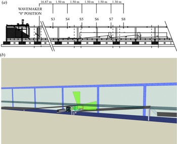
An experimental campaign has been devoted to the analysis of the vortex–vortex interaction over bed discontinuities. The framework was that of the project ‘FUNdamentals of BREAKing wave-induced boundary dynamics’ (FUNBREAK), that is aimed at better understanding the overall dynamics generated when breaking-induced vortices directly interact with near-bed coherent structures. The facility, hosted by the ‘Laboratory of Hydraulics and Maritime Construction’ (Università Politecnica delle Marche, Ancona, Italy), was a 50 m long, 1 m wide and with a 1.3 m deep flume (figure 1a). More details on the facility and some of the coastal models reproduced there are available in Lorenzoni et al. (Reference Lorenzoni, Soldini, Brocchini, Mancinelli, Postacchini, Seta and Corvaro2010, Reference Lorenzoni, Postacchini, Brocchini and Mancinelli2016) and Corvaro et al. (Reference Corvaro, Marini, Mancinelli, Lorenzoni and Brocchini2018).
(a) Wave flume of the Hydraulics and Maritime Construction Laboratory of the Università Politecnica delle Marche (Ancona, Italy), with indication of the wavemaker, physical model and gauge locations. (b) Detail of the investigated area.

The wave motion was forced by a piston-type wavemaker. An absorbing beach (slope  $1:20$) made of coarse gravel was used to reduce the wave reflection (estimated at approximately 5 %) and was fitted approximately 10 m shoreward of the study area. Therefore, since the duration of the recordings was of the order of (3–4) s, possible effects of the reflected wave on the measuring area were regarded as negligible. The sidewalls of the central part of the flume were glassed and enabled us to record and carry out optical measurements (e.g. Miozzi et al. Reference Miozzi, Postacchini, Corvaro and Brocchini2015).
The physical model thus represented an uneven seabed characterized by two sloping aluminium platforms (slope of  $1:10$, length of 3 m and width of 0.98 m each) over which waves travelled and broke. To allow for the generation of a near-bed vortex and its interaction with a breaking-induced surface vortex, discontinuities were reproduced at the seaward end of each platform using counter-sloping transparent plates (slope
 $1:1$). Further, the transparent plates enabled the generation of a laser sheet within the study area, fundamental for optical measurements (figure 1b).
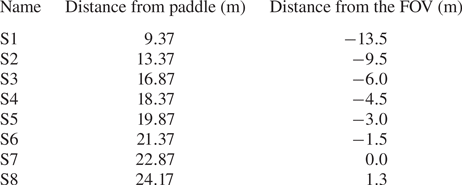
Eight electro-sensitive wave gauges recorded the surface level with a frequency of acquisition of 35 Hz, and thus the wave heights, at different streamwise locations of the flume (see table 1). The still water depth at the wavemaker was  $h_{swl}=40$ cm.
Distance of the free-surface gauges from the wave paddle and from the field of view (FOV).

To carry out optical measurements, two FLARE 12M125 CCD cameras with a resolution of  $4100\times 3072$ pixels and a 16-bit pixel depth were used, each allowing the recording of uncompressed images at
 ${\sim }125$ fps at full resolution on a dedicated DVR Express Core 2. The light source was a diode pumped, all-solid-state-laser by CNI, model MG. This green laser was capable of delivering a
 $4$ mm diameter,
 $10$ W beam, at a wavelength of
 $532$ nm in continuous wave mode. Use of this kind of laser, in conjunction with a high speed camera, has been already investigated successfully in Falchi & Romano (Reference Falchi and Romano2009), where small-scale features and statistics were evaluated against a standard particle image velocimetry acquisition system.
To properly seed the flow, hollow glass spheres were selected. The nominal diameter was  $10\,\mathrm {\mu }$m, while the specific weight was
 $1.1\,{\rm g}\,{\rm cm}^{-3}$. Based on these data and on the flow characteristics, the particle Stokes number was approximately equal to
 $10^{-4}$.
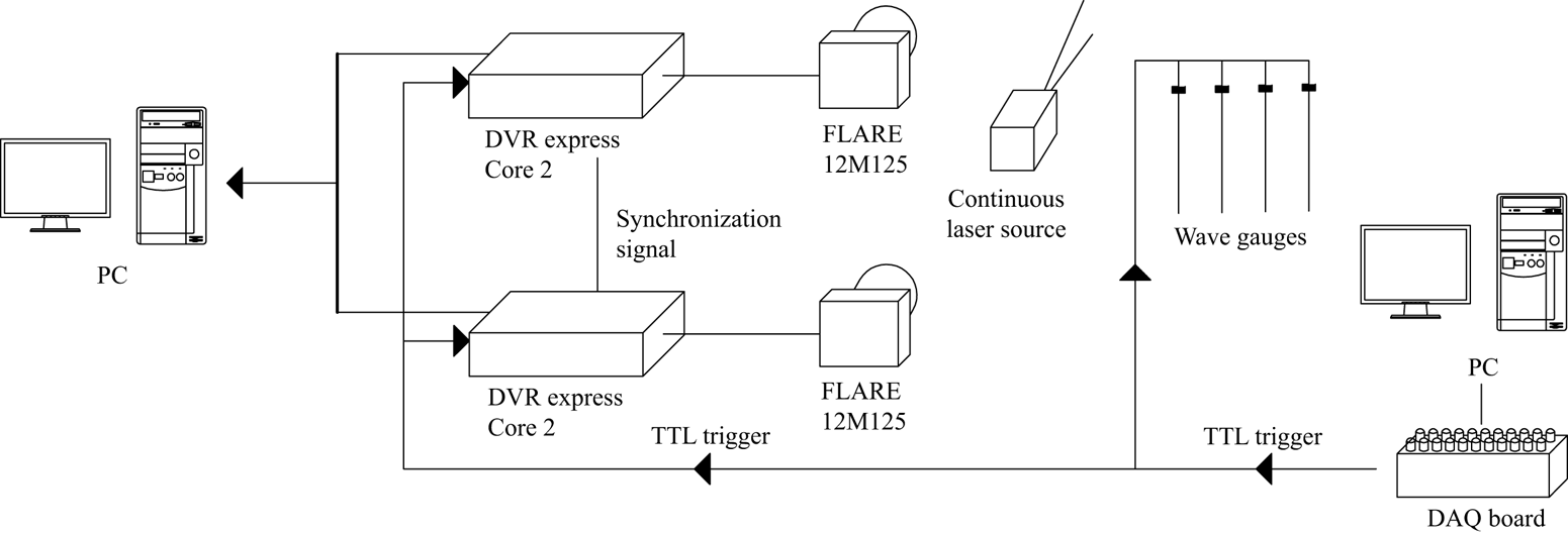
From a data acquisition board connected to the main computer, a TTL (transistor–transistor logic) trigger signal was sent both to the wave gauges and to the cores of the cameras to synchronize the data recordings. Subsequently, the optimal frame-by-frame synchronization of the images was obtained using another signal between the two cores. The laser source, being continuous, was not connected in this control system. For each test, the images taken from each camera were first stored in the core and then exported to a dedicated PC. A sketch of the set-up is illustrated in figure 2.
Layout of the electronic set-up and the triggering system.

2.2. Tested waves
Many wave conditions were tested at the beginning of the experimental campaign, characterized by either a plunging-type breaking, a spilling-type breaking or a backward breaking. However, spilling and plunging breakers resulted in no vortex–vortex interaction, as the near-bed vortex was rapidly washed away by the mean wave motion and only the breaking-induced vortex dominated the region just shoreward of the discontinuity. In addition, when plunging/spilling occurred exactly on the discontinuity, a large portion of the water body filled with air bubbles and, in such conditions, no particle tracking measurement was possible. Hence, twenty different wave conditions leading to backward breaking have been studied.
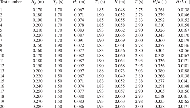
Waves were generated by imposing an external paddle displacement time series. Such a time series was not based on either solitary or cnoidal wave theories, but rather on the linear wave theory, with  $H_p$ and
 $T_p$ being the target wave height and period at the paddle (see table 2). Then, to reduce the presence of possible unwanted turbulent structures in the investigated area caused by start-up transient waves, the ramp-up time was reduced to only one wave period. Finally, the paddle was stopped once it reached its most forward position, this leading to the generation of only one regular wave, which allowed us to focus on a relatively simple vorticity field.
Wave characteristics imposed at the paddle ( $H_p$ and
 $T_p$) and measured at the wave gauge S1 (
 $H_1$ and
 $T_1$) and S6 (
 $H$ and
 $T$) and wave nonlinearity
 $H/h$ and steepness
 $H/L$.

During a preliminary testing phase, both the still water level  $h_{swl}$ and wave characteristics at the paddle (
 $H_p$,
 $T_p$) were chosen based on visualization of the flow field through the recorded images. Repeatability tests were performed through multiple runs of the same conditions, which showed that the overall behaviour of the large-scale vortices was properly captured and well repeated. After this phase, three different wave periods were selected (
 $T_p=1.5$, 1.7, 1.9 s) and a wave height range was chosen for each of them. Within each range, the intensity of the phenomenon changed from barely visible to a condition for which the air entrainment deviated the laser sheet, hindering the optical measurements.
The values of the wave characteristics imposed at the paddle and measured at wave gauges S1 ( $H_1$,
 $T_1$) and S6 (
 $H$,
 $T$) are summarized in table 2. Here, some relevant dimensionless wave parameters are also reported (
 $H/h$ and
 $H/L$), where
 $h$ was computed as the sum of the still water depth and the mean of the positive free-surface elevation at wave gauge S6, while
 $L$ is the wavelength computed through the linear wave theory. Therefore, the wave nonlinearity
 $H/h$ ranges from 0.26 to 0.38 while the wave steepness
 $H/L$ from 0.014 to 0.019.
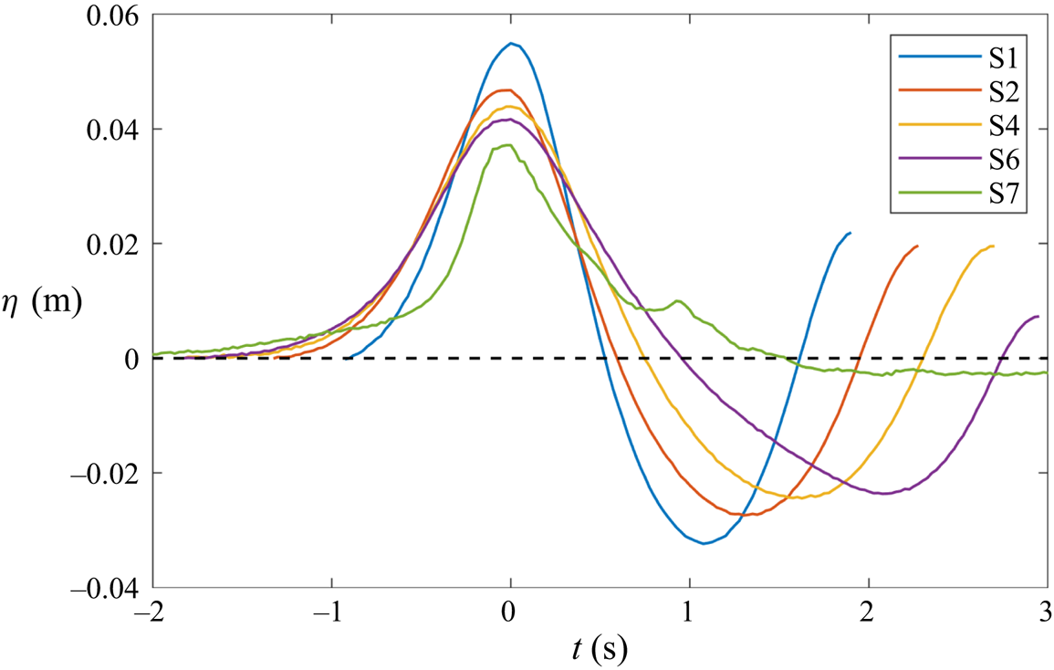
Figure 3 illustrates the time evolution of the free-surface elevation of the first generated wave at some representative wave gauges along the flume. This figure refers to Test 6, but the same behaviour was observed for all the other tests. The time origin is in correspondence with the wave crest. This allows for a better comparison of the shapes of the travelling wave among different wave gauges. The spurious part of the signal tail, after the second crest, has been omitted.
Example of free-surface propagation along the flume for Test 6.

After generation, before reaching wave gauges S6 and S7, the wave height decreases, while both wavelength and period increase. In addition, the measured wave period increases for increasing initial wave height, while it is weakly affected by the period at the paddle  $T_p$. Such behaviour is typical of solitary waves, for which the wave height is the main controlling parameter. However, the shape of the wave seaward of the discontinuity (from S1 to S6) remains comparable to that of a Stokes wave. On the contrary, in correspondence with the area of measurement (gauge S7), the wave is characterized by a solitary-wave shape, its surface being above the still water level for a long time. The second peak visible at time
 $t\approx 1$ s is ascribed to the backward breaking, which occurs after the passage of the wave crest. To obtain local information about the wave forcing the phenomenon, the characteristics of the waves at S6 (
 $H$,
 $T$) have been used in the following analysis.
2.3. Vortex characteristics
Following Leweke et al. (Reference Leweke, Le Dizes and Williamson2016), the vortices detected in the experiments have been characterized by concentrating the circulation of each vortex ( $\varGamma$) in its centre (
 $\boldsymbol {x}_c$)
 \begin{gather} \varGamma = \int_{\mathcal{S}} \omega \,{\rm d}\mathcal{S}, \end{gather}
 \begin{gather} \boldsymbol{x}_c = \frac{1}{\varGamma} \int_{\mathcal{S}} \boldsymbol{x} \omega \,{\rm d}\mathcal{S}, \end{gather}
where  $\mathcal {S}$ was the surface occupied by the vortex, which was detected using the vorticity field
 $| \omega | >2\,{\rm s}^{-1}$ in regions where
 $\lambda _{2}<0$,
 $\lambda _2$ being the second eigenvalue of the velocity gradient tensor. In particular, the two counter-rotating vortices were, respectively, defined as the one with the largest positive circulation
 $\varGamma ^+$ and the one with the largest negative circulation
 $\varGamma ^-$, among all the identified vortices. After such maxima were reached, each vortex was identified using the vorticity region (positive or negative) closer to the vortex centre evaluated in the previous frame. The correctness of this procedure was visually verified for all the tests and the results of stages characterized by a poor tracking (e.g. when the main vortex divides into smaller structures) were omitted. The radius of the vortex,
 $a$, was subsequently evaluated following Leweke et al. (Reference Leweke, Le Dizes and Williamson2016)
 \begin{equation} a^2 = \frac{1}{\varGamma} \int_{\mathcal{S}} \left| \boldsymbol{x} - \boldsymbol{x}_c \right|^2 \omega \,{\rm d}\mathcal{S}. \end{equation}
The kinetic energy  $E_{k}$ and the enstrophy
 $Z$ were defined as
 \begin{gather} E_{k} = \frac{1}{2} \int_{\mathcal{S}} \left| \boldsymbol{v} \right|^2 \,{\rm d}\mathcal{S}, \end{gather}
 \begin{gather} Z = \frac{1}{2} \int_{\mathcal{S}} \omega^2 \,{\rm d}\mathcal{S}, \end{gather}
where  $\boldsymbol {v}$ was the velocity field.
2.4. Visualizations and flow measurements
To fully detail the phenomenon under investigation, experimental tests were carried out following a two-step method. The wave condition of Test 6 in table 2 was chosen for the preliminary analysis on the tracking methods and on the filtering techniques. This specific test has been chosen because it was one of the most energetic, with a large wave height, wave period and velocities. In addition, the air entrainment during this test was negligible.
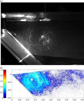
Visualizations have been preliminarily used to get qualitative, but nonetheless valuable, information about the overall characteristics of the interaction between the bottom and the surface vortex and its dependence on the wave time history and water depth. For this purpose, a first camera set-up was designed, using large exposure times ( $120$ ms) and a reduced frame rate (
 $8$ fps) at the full resolution of
 $4100\times 3072$ px (figure 4a).
Example of (a) vortex visualization and (b) reconstruction of the velocity field using the particle tracking velocimetry technique for Test 6.

As a second step, the two cameras were arranged one on top of the other (figure 1b) and the resolution of each of them was reduced to  $4100\times 850$ px, to achieve the larger frame rate of
 $435$ fps. This allowed us to reduce to 15 px the maximum displacement observed for the seeding particles between contiguous frames, and thus to perform an optimal tracking. The overlapping area between the two images was of the order of 5 %–10 % of the vertical dimension of each image. Before performing the particle tracking, images were pre-processed through stitching and background-subtraction operations. These led to a single-frame collection of images for each test, where reflections from both bottom and free surface were removed, as well as any other kind of residual background. The background removal algorithm was a sliding, time-minimum removal procedure in which the value to subtract, constantly updated, was evaluated over 20 consecutive images centred on the processed frame. This enabled us to enhance the particle image contrast and to increase to signal-to-noise ratio.
The origin of the reference frame has been placed at the highest point of the first set of ramps (see § 2.5). The FOV extends for around 0.46 m in the  $x$ direction and 0.18 m along y. The magnification factor, after calibration, is equal to
 $8.9\,{\rm px}\,{\rm mm}^{-1}$.
Tracking of the seeding particles was performed by means of the Part2Track software (Janke, Schwarze & Bauer Reference Janke, Schwarze and Bauer2020), which is an open sourceMATLAB package for double frame and time resolved particle tracking velocimetry. In order to handle high particle densities, a histogram matching method was used and a sub-pixel accurate detection of the tracer particles was achieved. The diameter of the particles was approximately 3 px. Since the cameras in use recorded with a bit depth of 16 bit, the maximum intensity of a single pixel ranged up to a value of 65 535. The particle detection intensity was set at 2000 counts. The field of the search was set at 30 px, i.e. twice the expected maximum displacement. Due to the average seeding density used, 0.05 ppp (particle per pixel), an error in the interval 1 %–2 % has affected the proposed velocity measurements, as evaluated in Janke et al. (Reference Janke, Schwarze and Bauer2020). An example of the tracked particles is given in figure 4(b), which shows both bottom and surface vortices. For each test, from the scattered results of the reconstructed trajectories, a structured velocity field with a grid spacing of 20 px has been deduced by the polynomial binning approach. Before computing the main parameters to characterize the vortical structures (§ 2.3), the structured velocity fields have been post-processed to perform a fast, reliable and automatic detection of the bottom and surface vortices, as well as of any other coherent structures that would form. To filter out the small-scale turbulence and to remove residual measurement noise, different approaches have been used to obtain vorticity fields characterized by a smooth evolution of the vortices without affecting the main quantities of interest, e.g. circulation, vortex radius, enstrophy. To this end, two different approaches have been tested: time-based and spatial-based analyses. A sliding, Gaussian filter and the snapshot proper orthogonal decomposition (POD) have been used to filter the data in time, while the wavelet transform has been used in the spatial domain. For each filtering technique, in addition, a fine tuning of the parameters has also been performed. In the following analysis, only the results with the best parameters have been reported. In more detail, the tested filtering approaches are:
(a) Gaussian time filter: the acquisition frequency in use was adequate to freeze the particle positions in the stored snapshots but over-sampled in comparison with the coherent structure time scale, the Gaussian-weighted moving average in time has been applied over a window of 35 time steps (included among the functions available in MATLAB);
(b) time-snapshot POD filter: in view of the reduced-order modelling, only the 50 most energetic modes have been used to reconstruct the instantaneous fields, on the assumption that these contained the largest coherent structures (included in the post-processing tools of the Part2Track software); and
(c) wavelet-based, multi-resolution analysis: instantaneous velocity fields have been decomposed up to the fifth level, a threshold has been applied to retain the largest coherent structures and the field has been reconstructed. In this view, in each velocity field, small and incoherent disturbances have been filtered out independently of the other instantaneous fields, differently from the two previous approaches.
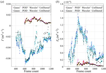
To evaluate the efficacy of all methods, the circulation and the kinetic energy of the vortices, described in § 2.3 have been compared for the reference wave conditions (Test 6) and the results are reported in figure 5, where unfiltered data are reported to evaluate the effectiveness of the proposed algorithms. The trends are quite similar for both  $\varGamma$ and
 $E_k$, although the application of the Gaussian filter seems to lead to smoother results (darker colours). Application of either POD or wavelet decomposition introduces more spikes. In addition, in comparison with the other methods, the Gaussian filter does not underestimate the maximum values. On the contrary, a small underprediction of the maxima has been obtained with the wavelet spatial filter. Therefore, the Gaussian time filter has been chosen to characterize the properties of the vortices, as discussed in § 3.
Comparison of the computed values of  $\varGamma$ (a) and
 $E_k$ (b) with different filtering techniques (Gauss, POD, wavelet) for both the clockwise (cold colours) and anticlockwise vortices (warm colours). Gauss: red and dark blue dots; POD: magenta and light blue; wavelet: orange and cyan; unfiltered: black.

2.5. Point-vortex analysis
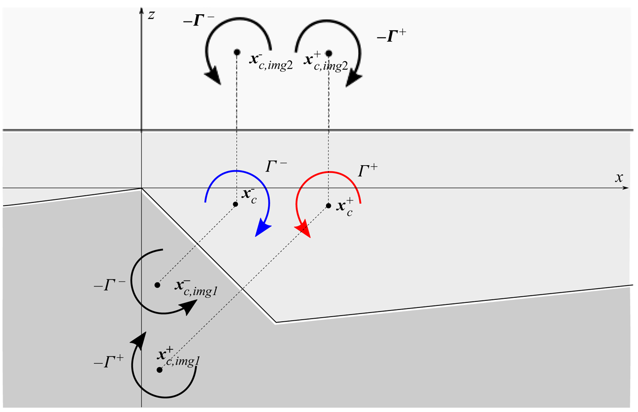
Considering the two-dimensional domain reported in figure 6, the interaction and migration of vortices due to mutual and self-advection can be simulated with the point-vortex method (Batchelor Reference Batchelor1971), used in the literature in finite domains with periodic boundary conditions to study the vortex–vortex interactions (Meunier, Le Dizes & Leweke Reference Meunier, Le Dizes and Leweke2005; Kuvshinov & Schep Reference Kuvshinov and Schep2016) and the interactions with the free surface (Curtis & Kalisch Reference Curtis and Kalisch2017). This approach has been used in various contexts: an example is the vortex ring theory applied to the dynamics of breaking-wave-induced macrovortices in the near shore (Bühler & Jacobson Reference Bühler and Jacobson2001; Brocchini et al. Reference Brocchini, Kennedy, Soldini and Mancinelli2004; Kennedy et al. Reference Kennedy, Brocchini, Soldini and Gutierrez2006; Terrile & Brocchini Reference Terrile and Brocchini2007). In our case, the point-vortex method has been used to reproduce the dynamics of the vortices due to mutual and self-advection only, using the available experimental data as initial conditions. The mutual advection of each vortex was given by the velocity field generated by the other vortex, evaluated using the Lamb–Oseen vortex theory suggested by Leweke et al. (Reference Leweke, Le Dizes and Williamson2016)
 \begin{equation} v_\theta = \frac{\varGamma}{2 {\rm \pi}r} [1 - {\rm e}^{({-r^2})/{a^2}}], \end{equation}
where  $r = | \boldsymbol {x} - \boldsymbol {x}_c|$ was the distance of the coordinate point
 $\boldsymbol {x}$ from the vortex centre
 $\boldsymbol {x}_c$ and
 $v_\theta$ was the velocity intensity, whose direction was perpendicular to
 $\boldsymbol {x} - \boldsymbol {x}_c$. Because of the complexity of the domain and boundary conditions, image vortices have been used to reproduce the self-advection due to the interaction with the seabed and with the free surface: this implemented the effect of the velocity field due to image vortices, characterized by an opposite circulation and a centre located symmetrically to the reference boundary, as depicted in figure 6. Since the model aimed at describing the evolution of the vortices in the absence of waves, the free surface was taken equal to the initial still water level. The initial location of the centre and the circulation of the vortices were extracted from the experiments by selecting an instant of complete development of the vortices. As the duration and intensity of the surface anticlockwise vortex are smaller than those of the bottom clockwise vortex, the initial condition was identified as the time when the largest circulation of the surface vortex was achieved. The analytical model was forced by such initial circulation, maintained constant during the subsequent vortex evolution. To compare with the experimental results, the theoretical motion of the two vortices was computed for the same time range and resolution of the experiments, considering three different cases:
(i) including only the mutual advection between the two vortices identified in the experiments (i.e. considering only the blue and red vortices in figure 6);
(ii) including the mutual advection between the two vortices identified in the experiments and the self-advection exerted by the seabed over each vortex (i.e. the effect on each vortex of the corresponding img1 vortex in figure 6); and
(iii) including the mutual advection between the two vortices identified in the experiments and the self-advection exerted by both the seabed and the free surface over each vortex (i.e. the effect on each vortex of the corresponding img1 and img2 vortices in figure 6).
The comparison of the results of the three different point-vortex models with the experimental results helps us to understand the role of the processes included in the models (mutual advection between the two vortices, the self-advection exerted by the seabed and the self-advection exerted by the free surface) with respect to the role of the neglected processes (e.g. mean wave flow or dissipative phenomena).
Sketch of the two-dimensional theoretical domain with the representation of the two counter-rotating vortices, coloured in blue and red, and their image vortices: vortices with indices img1 and img2 reproduce the contribution of the self-advection due to the interaction with the seabed and the surface, respectively.

3. Results
To better describe the results and make them portable, we use dimensionless variables. The time-averaged depth at gauge S6 (see figure 1), i.e.  $h$ as defined in § 2.2, is used as the vertical length scale, while the wavelength estimated at S6, i.e.
 $L$, is the horizontal length scale. Two velocity scales are used, i.e. the shallow water celerity
 $U_0=\sqrt {gh}$ and the maximum particle velocity
 $U_m=H/h\sqrt {g(H+h)}$ (e.g. Chang et al. Reference Chang, Hsu and Liu2005),
 $g$ being the gravitational acceleration. The time scale is given by the ratio between the length scale
 $h$ and the velocity scale
 $U_0$, which provides
 $\sqrt {h/g}$. The dimensionless variables are, thus, defined through a tilde
 $$\begin{gather} \tilde{t}=\frac{t}{\sqrt{h/g}},\quad\tilde{x}=\frac{x}{L},\quad\tilde{z}=\frac{z}{h},\quad \tilde{a}=\frac{a}{h},\quad\tilde{b}=\frac{b}{h},\quad \tilde{s}=\frac{s}{h}, \end{gather}$$
 $$\begin{gather}\tilde{\omega}=\frac{\omega}{\sqrt{g/h}},\quad\tilde{\varGamma}=\frac{\varGamma}{U_0h},\quad\tilde{Z}=\frac{Z}{U_0^2}, \quad\tilde{E}_k=\frac{E_k}{U_0^2h^2},\quad\tilde{\eta}=\frac{\eta}{h}, \end{gather}$$
 $$\begin{gather}Re=\frac{U_m h}{\nu},\quad Fr=\frac{U_m}{\sqrt{gh}}=\frac{U_m}{U_0}, \end{gather}$$
where  $(x,z)$ represents the coordinate system,
 $a$ is the vortex radius,
 $b$ is the distance between the vortex cores,
 $s$ is the vortex distance from the origin of the Cartesian system
 $(x_0,z_0)=(0,0)$ and
 $\eta$ is the free-surface elevation. Further,
 $Z$ represents the enstrophy,
 $E_k$ the vortex kinetic energy,
 $\nu =10^{-6}\,{\rm m}^2\,{\rm s}^{-1}$ the water kinematic viscosity.
3.1. Vortex generation and evolution
Among all the tested waves, three wave conditions are chosen as representative of three main nonlinearity classes, to highlight how the generation and evolution of both surface and bottom vortices are related to the main dimensionless parameters. In particular, such tests are selected to represent a weak/medium/strong interaction between the vortices associated with the lowest/medium/largest values of  $H/h$ and
 $H/L$, within the tested range. In agreement with the vortex-path evolution observed for all tests (see § 3.2), the wave conditions used for the analyses that follow are (see also table 2):
(a) Test 15: weak interaction –
 $H/h$=0.277; $H/L$=0.014;
(b) Test 5: medium interaction –
$H/h$=0.326; $H/L$=0.017; and(c) Test 7: strong interaction –
$H/h$=0.360; $H/L$=0.018.


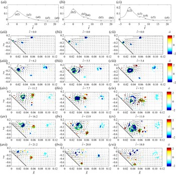
The evolution of the vortical structures, identified as described in § 2.3, is evident from the representative phases reported in figure 7, for each of the selected tests. In the first row, the free surface of the three tests measured at wave gauge S7 is reported. In the remaining panels, the vortex boundary is highlighted by a continuous green line ( $\tilde {\omega }\approx -0.27$ for the clockwise vortex and
 $\tilde {\omega }\approx 0.27$ for the counter-clockwise vortex, corresponding to the dimensional threshold defined in § 2.3).
Vorticity fields filtered with  $\lambda _2<0$ during five different time frames: (a) Test 15 (
 $H/h=0.277$), (b) Test 5 (
 $H/h=0.326$) and (c) Test 7 (
 $H/h=0.360$). (a i,b i,c i) Free surface measured at wave gauge S7; (a ii–c vi) panels not evenly spaced in time, but selected at the most representative phases of the phenomenon.

During a first phase, a clockwise (negative) near-bed vortex is generated, due to the large horizontal velocities under the wave crest (rows 2 and 3 of figure 7) seaward of the seabed change of slope. In a second phase a counter-clockwise vortex is generated in at the position of backward breaking and entered the measuring area (row 4 of figure 7). Next, some interactions occur (row 5 of figure 7) and finally the vortices dissipate and/or move outside the FOV (row 6 of figure 7). Within this common behaviour, some differences are discussed. First, the size of the vortices increases for the most energetic wave conditions with different trends for the near-bed and for the surface vortices. The clockwise vortex in the left panels (figure 7a) is rather small. A slightly larger nonlinearity provides a marked size increase (figure 7b). At this point, a more energetic wave condition (figure 7c) does not generate a significantly larger vortex. On the contrary, the size of the counter-clockwise surface vortex increases more than the near-bed one moving from Test 5 to Test 7 (figure 7b,c). As a consequence, for the waves with the smaller nonlinearity (or steepness) the size of the bottom clockwise vortex is always 2–3 times larger than that of the surface vortex. For the most nonlinear wave condition, the sizes of the vortices are comparable. Such behaviour is due to the increase of the wave height and breaking intensity, which scales with the vortex size.
For all the tests, another coherent structure with negative vorticity can be identified in the top right part of the FOV. Such a vortex is generated during the passage of the wave crest at gauge S7 ( $\tilde {t}\approx 0$) by the interaction of the incoming near-surface horizontal flow with the quiescent water region located shoreward of the discontinuity, which induces a shearing effect, and by the water depth that rapidly changes from 4 to 25 cm (figure 7a i,b i,c i). Specifically, the shear layer is aligned orthogonally to the counter-slope and moves in the downward–shoreward direction during the passage of the wave crest (rows 1–2 of figure 7). After this phase (
 $\tilde {t}\gtrsim 6$) all vortices keep a stable position, with the farthest structure in the top right area (
 $\tilde {x}\approx 0.10$) appearing to be unaffected by the presence of the other vortices. The smaller shearing vortices are mostly dissipated before the generation of the two main counter-rotating vortices and their contribution to the overall phenomenon is regarded as negligible, they are thus not studied in detail in the present work.
The analysis of the velocity and vorticity fields leads to a qualitative study of the vortex breakdown process. Three main classes are identified depending on the wave nonlinearity  $H/h$ and the three wave conditions reported in figure 7 can be taken as representative of such classes.
When the flow is quite weak ( $H/h\lesssim 0.30$), the size of the vortices is rather small compared with their distance, the structures remain coherent during their motion and no evident increase in size nor breakdown occurs before the vortices move outside the FOV (figure 7a). In such a regime, a small interaction between the vortices occurs, with the surface vortex remaining near the centre of the FOV for a long time and its intensity and size remaining almost constant, (e.g. see figure 7a iv,a v). The bottom vortex, generated at the illumination limit (figure 7a ii), remains unaltered for the first three phases and then moves upward and seaward because of the backflow of the incoming wave tail, up to the point it completely disappears (figure 7a v).
When the flow intensity increases ( $0.30\lesssim H/h \lesssim 0.33$), the bottom vortex increases in size, remains coherent for a long time (figure 7b i–b iii) and slightly expands in the phases that follow (figure 7b v). The surface vortex is less coherent and, even if this effect is not very evident in figure 7(b), some patches detach from the main body of the vortex before its breakdown. Specifically, when the surface vortex is generated (figure 7b iii), the distance from the bottom vortex is small, leading to a large interaction and to an instability of the surface vortex, which breaks down into smaller structures (figure 7 b iv). A region where positive and negative vorticity patches are dispersed is observed during the final phases, in which the bottom vortex moves, again, seaward after a small fragmentation of the vortex occurs (figure 7b v,b vi).
The third class ( $H/h\gtrsim 0.33$) is characterized by larger and closer vortices, with the surface vortex moving around the bottom vortex (figure 7c). Here, the size of both vortices starts to increase at an earlier stage (
 $\tilde {t}\approx 8\text {--}12$) while their vorticity decreases. The surface vortex is more energetic than that observed in the previous classes, and forces the breakdown of the bottom vortex. This happens because both vortices break into smaller vortices that mix up, strongly interact and allow their breakdown to occur faster.
Although our experimental set-up only allows for measurement of two-dimensional (2-D) vortical structures, our visual observation suggests the flow is also characterized by some 3-D structures. These seem to differ from the ‘obliquely descending eddies’, first described in Nadaoka, Hino & Koyano (Reference Nadaoka, Hino and Koyano1989) and typically generated by spilling and plunging breakers. In the scenarios we analyse here, i.e. characterized by a backward breaking with reduced splash down and significant near-surface shearing, some downward-evolving 3-D vortices seem to evolve, likely generated by the instability of the 2-D vortices measured here. For this purpose, a specific analysis by means of dedicated numerical simulations is being carried out, whose results will be summarized in Part 2 of this effort.
3.2. Evolution of vortex characteristics
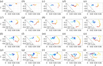
The experimental tracking of the positive and negative vortices sorted by increasing  $H/h$ is illustrated in figure 8. The results confirm that the motion of the core of the bottom clockwise vortex is initially shoreward (light blue parts of the tracks), then it slows down and remains in a steady position and, in some cases, it returns seaward. No relevant differences in such behaviour are evident for increasing nonlinearity (
 $H/h$), even if larger nonlinearities are associated with larger shoreward motions. Some of the paths are characterized by abrupt discontinuities (e.g. figure 8q,t), since the vortex-tracking code ‘follows’ the main circulation region but cannot easily identify the core when the vortex breaks into many unconnected regions (e.g. see figure 7c iii–c v).
Evolution of the centre of the vortices, sorted by increasing  $H/h$. Cold colours, from light to dark blue, represent the path of the clockwise vortex, while warm colours, from yellow to red, represent the path of the anticlockwise vortex.

The surface anticlockwise vortex is always generated more shoreward than the bottom clockwise vortex and it moves around the other vortex in most of the experiments: the motion starts in the downward/shoreward direction and changes into a downward/seaward direction and, in some cases, into an upward/seaward direction. Also, the motion of the core of the surface anticlockwise vortex becomes longer for increasing nonlinearity.
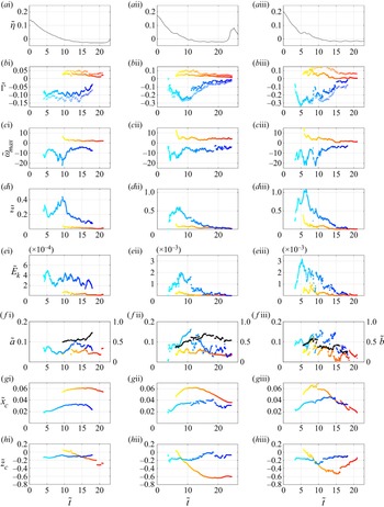
The time evolution of the vortex characteristics is reported in figure 9 for the three representative experiments, characterized by increasing nonlinearity. The results of the remaining tests are reported as online supplementary material available at https://doi.org/10.1017/jfm.2022.260. The experimental results are characterized by a large variability in time, but we can recognize the increasing–decreasing evolution of the circulations of both vortices, testifying to their formation and dissipation. In all the experiments, the bottom clockwise vortex is generated before the surface anticlockwise vortex and maintains a significant intensity for a longer period (on average  $| \varGamma ^-|_{max} \simeq 3 | \varGamma ^+|_{max}$).
Time evolution of the free-surface elevations (a i–a iii) at gauge S7 and of the vortex characteristics in Test 15, characterized by  $H/h=0.277$ (a i,b i,c i,d i,e i, f i,g i,h i), Test 5, characterized by
 $H/h=0.326$ (a ii,b ii,c ii,d ii,e ii, f ii,g ii,h ii) and Test 7, characterized by
 $H/h=0.360$ (a iii,b iii,c iii,d iii,e iii, f iii,g iii,h iii). Cold colours (from light to dark blue) are used for the clockwise vortex, while warm colours (from yellow to red) are used for the anticlockwise vortex. The crosses in panels
 $b^*$ represent the positive (warm colours) and negative (cold colours) total circulations. Black dots in panels
 $f^*$ represent the distance between the vortex centres.

In figure 9(b), two sets of data for each vortex are shown: the dots give the circulation of both vortices as described in § 2.3, while the crosses represent the overall positive and negative circulations, evaluated following the approach of Gharib, Rambod & Shariff (Reference Gharib, Rambod and Shariff1998), over a large area of the measured domain, delimited by  $\tilde {x}\leq 0.55$ and
 $\tilde {z} > z_b +2$ mm, where
 $z_b$ is the seabed location (using such a domain, the overall circulation does not include the circulation of far shoreward vortices and that due to the seabed shearing). In the case of smaller nonlinearity (figure 9b i) both positive and negative overall circulations largely differ from the positive and negative vortex circulations, even if the difference remains almost constant in time. This is because the vortices are not very energetic and the contribution of the surrounding vorticity to the overall circulation is significant. Conversely, the cases with larger nonlinearity (figure 9b ii,b iii) are characterized by a first phase in which the overall clockwise circulation in the domain (sum of all same signed contributions) is close to the bottom clockwise vortex circulation. Subsequently, at
 $\tilde {t}\approx 10$, the bottom clockwise vortex circulation drops and evolves with a larger difference from the overall circulation. The decay of the bottom-vortex circulation is not monotonic, mainly for the most energetic tests (e.g. see figure 9b iii). After reaching its maximum (at
 $\tilde {t}\approx 5$),
 $|\varGamma ^-|$ decays, with fluctuations evident for
 $\tilde {t}\approx 5-10$. Such fluctuations are likely due to the interaction of the vortex with the breaking-induced jet. In particular, the small but defined coherent structures generated in the left region of the jet are driven initially by the jet itself, following its trajectory, and then captured by the bottom vortex. The subsequent merging of such small vorticity patches with the bottom vortex leads to a temporary increase of vorticity and circulation values, resulting in the measured fluctuations (figure 9b iii,c iii).
The initial circulation of the surface vortex is close to the overall positive circulation, but it suddenly drops down to reach a quasi-steady evolution. Such a drop is representative of the vortex breakup, proving the loss of circulation of the main structures and the subsequent evolution of less intense, persistent structures.
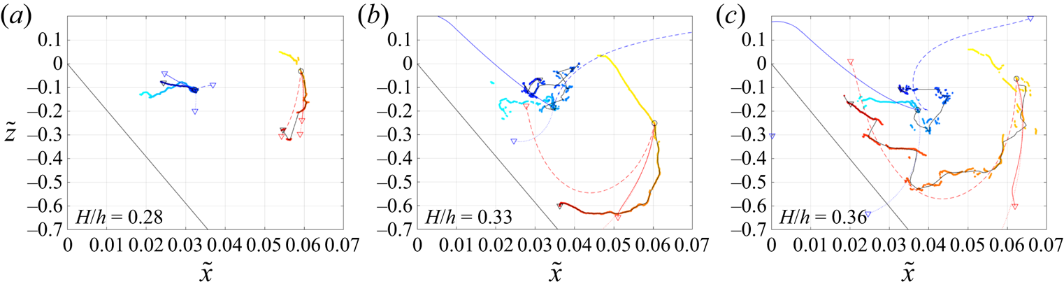
Figure 10 illustrates the results of the point-vortex model, superimposed on the experimental results, for the three reference tests. In all panels, three theoretical paths are included, each indicating a different modelling approach (see § 2.5), i.e. (i) only mutual advection (dotted lines), (ii) mutual advection and self-advection due to seabed (solid lines) and (iii) mutual advection and self-advection due to seabed and surface (dashed lines). All theoretical paths of the surface anticlockwise vortex are similar and in good agreement with the experimental results, that of case (iii) providing the best results. Conversely, large differences are highlighted in the theoretical paths of the bottom vortex for the three modelling approaches: (i) for mutual advection only, the bottom vortex moves downward, with a seaward curvature for the cases with the highest nonlinearity; (ii) for mutual advection and self-advection due to the seabed, the bottom vortex moves upward and seaward, because of the dominant effect of the self-advection due to the seabed, (iii) for mutual advection and self-advection due to seabed and water surface, the bottom vortex moves in different manners: upward and shoreward, with an initial nose-shape motion for the case with the highest nonlinearity. Generally, the surface-vortex path seems to be fairly well captured by the point-vortex model, while the bottom-vortex motion is fairly well described by the point-vortex model only for small nonlinearities. This suggests a very different influence of the mean wave flow onto the two vortices, which is discussed in § 4.
Evolution of the position of the centres of the vortices: (a) Test 15; (b) Test 5; (c) Test 7. Cold colours, from light to dark blue, represent the time evolution of the centre of the clockwise vortex, while warm colours, from yellow to red, represent the time evolution of the centre of the anticlockwise vortex. The sharp black lines represent the time-averaged experimental trajectories, obtained with a 50 frame (i.e. 0.115 s) moving average, and initial time corresponding to the initial condition used for the point-vortex model (circle). Coloured sharp lines represent the theoretical evolution, predicted by the point-vortex model with different contributions: (i) only mutual advection (dotted lines), (ii) mutual advection and self-advection due to seabed (solid lines) and (iii) mutual advection and self-advection due to seabed and surface (dashed lines). All trajectories start with a circle symbol and end with a triangle symbol.

3.3. Maximum values of vortex characteristics
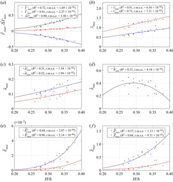
Concerning all 20 tests carried out during the campaign, relevant and synthetic quantities are extracted to describe the behaviour of the vortex pair for different wave conditions. Specifically, the maximum (or minimum) values of such quantities observed during the entire duration of each test are extracted for both vortices (blue for the clockwise bottom vortex, red for the anticlockwise surface vortex). The aggregated values coming from all tests are given in the dimensionless form in figure 11 as a function of the wave nonlinearity  $H/h$, which also describes their goodness of fit through the coefficient of determination (
 $R^2$) and the root-mean-square error (r.m.s.e.). Analysis of the data has shown that the most suitable best fit laws are of polynomial type i.e.
 $y=\sum _n \alpha _n x^n$.
Dimensionless maximum quantities of the clockwise/bottom (blue) and anticlockwise/surface (red) vortices from all tested configurations as function of  $H/h$: (a) circulation of both vortices and circulation difference (black); (b) distance between vortex core and origin of the reference frame; (c) vortex radius; (d) distance between vortex cores (black); (e) maximum vortex energy; ( f) maximum vortex enstrophy.

The maximum circulation is illustrated in figure 11(a), where the clockwise bottom vortex is reproduced by blue dots ( $\tilde {\varGamma }^-_{max}$) and the anticlockwise surface vortex is shown by red dots (
 $\tilde {\varGamma }^+_{max}$). The function
 $y=\alpha _3 x^3$ reproduces well the relationship between the normalized maximum circulation and the wave nonlinearity, with
 $R^2>70\,\%$ for both vortices (blue and red lines). The circulation difference (
 $\tilde {\Delta \varGamma }_{max}=\tilde {\varGamma }^+_{max}-\tilde {\varGamma }^-_{max}$) is also well described by the same function (black dots and line).
Figure 11(b–d) illustrates the maximum distance of each vortex core from the system origin ( $\tilde {s}^+_{max}$,
 $\tilde {s}^-_{max}$), the maximum vortex radius (
 $\tilde {a}^+_{max}$,
 $\tilde {a}^-_{max}$) and the minimum distance between vortex cores (
 $\tilde {b}_{max}$). Although the fit is not completely satisfactory for
 $\tilde {b}_{min}$, all data series show an increasing dependence on
 $H/h$, with the vortex distance from the origin and the radius, both characterized by a fairly good fit, i.e.
 $R^2>50\,\%$. While the quadratic law
 $y=\alpha _2 x^2+\alpha _1 x+\alpha _0$ is used to fit both
 $\tilde {a}_{max}$ and
 $\tilde {b}_{max}$, a linear trend
 $y=\alpha _1 x$ is used for
 $\tilde {s}_{max}$.
The normalized maximum kinetic energy of each vortex  $\tilde {E}_{max}$ (figure 11e) also increases with
 $H/h$, with a fairly high fitting degree (
 $R^2>68\,\%$). Similarly, the normalized enstrophy
 $\tilde {Z}_{max}$ (figure 11f) increases with the nonlinearity and shows a good fit for both vortices (
 $R^2>57\,\%$). The above normalized quantities are fitted using the law
 $y=\alpha _n x^n$, with
 $n=6$ for the vortex energy and
 $n=4$ for the enstrophy.
Figure 12 shows the dependence of the absolute vorticity on both the Reynolds number  $Re$ and Froude number
 $Fr$. The surface anticlockwise vortex seems to be relatively well described (
 $R^2>60\,\%$) by
 $y=\alpha _n x^n$, with
 $n=2$, while the bottom vortex is described by a larger data scatter, although the vorticity intensity increases with both
 $Re$ and
 $Fr$. Despite the data scatter and the non-optimal fit, the present results for the bottom vortex are consistent with what was observed by Chang et al. (Reference Chang, Hsu and Liu2005), who documented an almost linear increase of the normalized maximum vorticity with
 $Re$, although they used slightly different scales for the normalization and their fitting line did not intersect the origin of the Cartesian axis.
Normalized vortex intensity plotted against  $Re$ (a) and
 $Fr$ (b).

Going back to dimensional quantities by means of (3.1a–f), the above fitting laws suggest the following:
 $$\begin{gather} \varGamma^\pm_{max} \varpropto \left(\frac{H^2}{h}\right)^{3/2}; \quad \Delta\varGamma_{max} \varpropto \left(\frac{H^2}{h}\right)^{3/2}, \end{gather}$$
 $$\begin{gather}s^\pm_{max} \varpropto H ;\quad a^\pm_{max} \varpropto H, \end{gather}$$
 $$\begin{gather}E^\pm_{max} \varpropto \left(\frac{H^2}{h}\right)^3, \end{gather}$$
 $$\begin{gather}Z^+_{max} \varpropto \frac{H^4}{h^3};\quad Z^-_{max} \varpropto \frac{H^4}{h^3}. \end{gather}$$
Specifically, although the best fit for the radius is provided by the quadratic polynomial  $y=\alpha _2 x^2+\alpha _1 x+\alpha _0$, with
 $\alpha _0=0,\alpha _1\neq 0,\alpha _2\neq 0$, it can be proved that
 $\tilde {a}_{max}$ depends more on
 $H/h$ than on
 $(H/h)^2$, with coefficients of determination
 $R^2$ slightly smaller than those previously obtained (figure 11c). Hence, all the above quantities strongly depend on the local wave height and some of them, to a lesser extent, on the local water depth. It is to be stressed that the vortex radius and the vortex distance from the origin are almost completely governed by the wave height.
3.4. Vortex instability
We here provide some qualitative insight into the role played by instabilities in the dynamics of the vortex interaction and breakdown. A quantitative analysis of instability cannot be performed based on the available experimental data, collected over a vertical plane of the flow.
As documented in the literature (e.g. Leweke & Williamson Reference Leweke and Williamson1998; Fabre, Jacquin & Loof Reference Fabre, Jacquin and Loof2002; Leweke et al. Reference Leweke, Le Dizes and Williamson2016), the interaction of opposite, unequal strength vortices may lead to both elliptic (short-wave) and Crow (long-wave) instabilities. Such investigations have been performed in freely evolving conditions, different from the present experiment, where the wave-breaking-generated jet and the rigid boundaries of the flume largely influence the dynamics. In this framework, our analysis can only be qualitative (as we only measured the main quantities on the vertical plane, with no information about the spanwise wavelength).
The time oscillations of some vortex properties and the vortex breakdown can be associated with instability phenomena. Hence, some parameters that are typically used for the description of short-wave and long-wave instabilities valid for counter-rotating vortices (Leweke et al. Reference Leweke, Le Dizes and Williamson2016) are computed for the three reference tests. Since the potential for the vortex pairs to become unstable increases with the increase of the radius-to-core-distance ratio  $\tilde {a}/\tilde {b}$, its time evolution is shown in figure 13(a–c). Further, assuming that the instability growth rate
 $\sigma$ of a vortex is proportional to the normalized circulation
 $\tilde {\varGamma }/\tilde {b}^2$ for both instability types (e.g. see the classical analytical formulations shown in Leweke et al. Reference Leweke, Le Dizes and Williamson2016),
 $\tilde {\varGamma }/\tilde {b}^2$ is illustrated in figure 13(d–f).
Time evolution of  $\tilde {a}/\tilde {b}$ (a–c) and
 $\tilde {\varGamma }/\tilde {b}$ (d–f) for Test 15 (
 $H/h=0.277$, blue), Test 5 (
 $H/h=0.326$, orange), Test 7 (
 $H/h=0.360$, yellow).

All panels show a smooth evolution in the case of the smallest nonlinearity for all the three analysed terms (blue dots), while a larger nonlinearity leads to the generation (orange dots) and increase (yellow dots) of oscillations during the evolution. This suggests that relatively small nonlinearities are characterized by almost stable values of both radius and core distance (see § 3.2 and figure 9), while relatively large nonlinearities force the vortices to alternatively move closer and further apart, testifying to an unstable behaviour. For Test with  $H/h=0.360$ (yellow dots) the instability is confirmed by the evolution of
 $\tilde {\varGamma }/\tilde {b}^2$ (figure 13d–f), which shows much larger oscillations than the cases with smaller nonlinearity.
As shown, the local maxima of  $\tilde {a}/\tilde {b}$ and
 $\tilde {\varGamma }/\tilde {b}^2$ are not always occurring at the same time and their time evolution is rather different. As an example, for the case
 $H/h=0.360$, the instability is more likely to occur at
 $\tilde {t}\approx 34, 38, 42$, when
 $\tilde {a}/\tilde {b}$ reaches its maximum values (figure 13a–c). On the other hand, the maximum growth rate is expected to occur at
 $\tilde {t}\approx 34$, when
 $|\tilde {\varGamma }/\tilde {b}^2|$ is larger than that evaluated at
 $\tilde {t}\approx 38$ and much larger than that evaluated at
 $\tilde {t}\approx 42$ (figure 13d–f).
The present experimental set-up and geometry allows for the emergence of both short-wave instability (perturbation lengths of the same order as the core distance  $b$) and long-wave instability (perturbation lengths up to ten times
 $b$). Specifically, assuming a ratio
 $a/b\approx 0.1$ (figure 13a–c) and a core distance
 $b\approx 0.1$m (figure 9f), the Crow instability occurs at
 $\lambda /b>6$ (Leweke et al. Reference Leweke, Le Dizes and Williamson2016), corresponding to
 $\lambda >0.6$ m, which is smaller than the flume width. Hence, we cannot exclude the existence of the long-wave instability and both types of instability can, in principle, evolve in this flow. However, such instabilities can only be speculated using the parameters available from our present analysis, which do not provide information on the spanwise flow evolution. To clarify the role of long- and short-wave instability, a 3-D approach is needed and represent the natural extension of the present work.
4. Discussion
Our experiments have highlighted the generation of a pair of large-scale, counter-rotating vortices, as a result of the propagation of a single regular wave over a sloping platform followed by an abrupt discontinuity. The bottom vortex is characterized by a shoreward–upward/seaward migration similar to that of the bottom vortex observed when solitary or cnoidal waves travel over rectangular submerged structures, in the case of both breaking and non-breaking waves (e.g. Chang et al. Reference Chang, Hsu and Liu2005; Wu et al. Reference Wu, Hsiao, Huang and Hwang2012). Conversely, the surface vortex behaves differently depending on the nonlinearity.
The three identified classes of increasing wave nonlinearity, i.e.  $H/h=(0.26-0.30)$,
 $H/h=(0.30-0.33)$ and
 $H/h=(0.33-0.38)$, are characterized by maximum quantities (figure 11) that increase with the nonlinearity, sometimes by several orders of magnitude. Specifically, passing from the first to the second to the third class, the maximum normalized values of both circulation
 $\tilde {\varGamma }_{max}$ and circulation difference
 $\tilde {\Delta \varGamma }_{max}$ (figure 11a) are double and triple, respectively. In the case of the maximum distance
 $\tilde {s}_{max}$ (figure 11b) and maximum normalized radius
 $\tilde {a}_{max}$ (figure 11c), the values increase by, respectively,
 ${\sim }35\,\%$ and
 ${\sim }15\,\%$. Much larger is the increase of the maximum energy
 $\tilde {E}_{max}$ (figure 11e), where the relationship among the values of the first, second and third classes is approximately
 $1:2.5:5.5$, while the relationship in the case of the normalized maximum enstrophy
 $\tilde {Z}_{max}$ (figure 11f) is
 $1:2:4$ (surface vortex) and
 $1:1.5:2.5$ (bottom vortex). Hence, the increase of maximum vortex properties increases (in absolute value) with the wave nonlinearity, suggesting an increase of the interaction between the counter-rotating vortices when moving from the first to the third class. This interaction is also supported by a general decrease of the minimum distance between the vortex cores
 $\tilde {b}$ with
 $H/h$ (figure 11d). In summary, the larger the wave nonlinearity is, the greater are the vortices, the smaller is their distance, the larger are the circulation, energy and enstrophy and the larger is their interaction.
Also the surface-vortex dynamics shows different characteristics for each different class. The surface vortices of the first class, characterized by the smallest nonlinearities ( $H/h\sim (0.26\text {--}0.30)$), are more confined in the upper water column (the core reaching a maximum depth
 $\tilde {z}\sim -0.4$) and probably slightly affected by the interaction with the bottom vortex, which does not allow the surface vortex to keep moving downward but forces it to move seaward. In this condition, the time evolution of the main vortex characteristics for the case with
 $H/h=0.277$ (left panels in figure 9) suggests that the surface vortex is characterized by almost constant flow/kinematic properties (
 $\tilde {\omega }_{max}$,
 $\tilde {\varGamma }$,
 $\tilde {E}$,
 $\tilde {Z}$), while the geometry changes and seems to be affected by the bottom vortex (see
 $\tilde {a}$ and
 $\tilde {b}$). Specifically, while the kinematic properties of the bottom vortex present an irregular time evolution for
 $\tilde {t}<10$, the presence of the surface vortex seems to increase/decrease the maximum vorticity/enstrophy of the bottom vortex (
 $\tilde {t}\sim (10\text {--}13)$) and makes it almost constant (
 $\tilde {t}>13$). Further, the radius
 $\tilde {a}$ of both vortices seems to be affected by their mutual interaction, both radii increasing just after the surface-vortex release (
 $\tilde {t}\sim 10$), followed by a stage during which the bottom-vortex radius increases on average while the surface-vortex radius decreases on average (
 $\tilde {t}\sim (12\text {--}13)$). The opposite behaviour (decrease/increase for bottom-/surface-vortex radius) occurs at
 $\tilde {t}\sim (13\text {--}16)$, this changing again (increase/decrease for bottom-/surface-vortex radius) at
 $\tilde {t}\sim (16\text {--}17)$ and again (decrease/increase for bottom-/surface-vortex radius) at
 $\tilde {t}\sim (17\text {--}18)$, up to the disappearance of the bottom vortex. A rapid increase of the vortex distance
 $\tilde {b}$ characterizes the two latest stages, i.e. during
 $\tilde {t}\sim (16\text {--}18)$, this also reduces the mutual interaction between the vortices. Application of the point-vortex model reveals that, for small nonlinearities, the surface-vortex path is clearly driven by the mutual advection with the larger bottom vortex, which dominates over all other mechanisms (figure 10a).
Almost circular paths are followed by surface vortices of the second class, with medium nonlinearity i.e.  $H/h\sim (0.30\text {--}0.33)$, initially moving downward and shoreward, then seaward. In some tests, the vortex core reaches a deeper portion of the water column (down to
 $\tilde {z}\sim -0.8$), interacts with the nearby vortical patches and the mean motion, but rarely reaches the seabed and the point-vortex model clearly shows that such motion is triggered by both mutual interaction with the bottom vortex and self-advection due to both free surface and seabed (figure 10b). Similarly to what was observed for smaller nonlinearities, most of the surface-vortex properties do not change significantly, like those of the bottom vortex. Conversely, the absolute values of both maximum vorticity and enstrophy of the bottom vortex decrease just after the appearance of the surface vortex (at
 $\tilde {t}\sim 6$), while an abrupt increase occurs for radius, circulation and energy. Such quantities decrease after some time (
 $\tilde {t}\sim 8$), with
 $\tilde {a}$,
 $\tilde {\varGamma }$ and
 $\tilde {E}$ gradually decaying and reaching values close to those characterizing the surface vortex. Differently from the previous example, the size of the surface vortex seems to be unaffected by the bottom-vortex change, despite both cases are characterized by similar distances between the cores, i.e.
 $\tilde {b}\sim 0.5$ when the bottom-surface radius is maximum (compare panels ( f u) and ( f ii) in figure 9).
Finally, waves with even larger nonlinearity, i.e.  $H/h\sim (0.33\text {--}0.38)$, generate surface vortices characterized by more pronounced circular paths, with a quite clear seaward and upward motion after the initial downward–shoreward phase. In this case, the interaction with the seabed lasts longer, thus suggesting that the self-advection mechanism plays an important role, as confirmed by the point-vortex model (figure 10c). Test
 $H/h=0.360$ displays (right panels in figure 9) some similarities to the smaller nonlinearity classes, e.g.
 $|\tilde {\varGamma }|$,
 $\tilde {E}$ and
 $\tilde {Z}$ of the bottom vortex begin to decay when the surface vortex comes into the domain. However, differently from the other classes, the sizes of both vortices are significantly close to each other and rapidly evolve in time, during the whole test, suggesting a strong interaction between the two, which is also confirmed by the smaller core distance (compare panels ( f i), ( f ii) and ( f iii) in figure 9). This can also be observed in figure 8, where the surface vortex approaches the ground and climbs the counter-slope while moving seaward, thus getting closer to the bottom vortex.
A fundamental result is that the motion of the surface vortex is driven by both mutual interaction and self-advection, the latter increasing its role with larger wave nonlinearity, while the jet and the mean wave motion have a negligible effect on the evolution of the surface-vortex motion, at least before the vortex breakup. On the other hand, it has been seen that the breaking-induced jet significantly affects the circulation of the bottom vortex, inducing some fluctuations before the beginning of circulation decay.
On the other hand, the bottom-vortex motion shows an alternating seaward/shoreward and upward/downward with no evident differences among the three classes of tests and such motion, although the vortex does not migrate much seaward during the negative wave phases, defying the typical evolution of previous laboratory experiments (e.g. Chang et al. Reference Chang, Hsu and Liu2005). In particular, comparing the experimental evolution of the centres in figure 8 we find that for the least nonlinear waves (first class,  $H/h<0.30$), the seaward motion is more frequent (see figure 8c–h) than for the largest nonlinearities (third class,
 $H/h>0.33$), where the shoreward motion is more evident (see figure 8q–t).
The bottom-vortex motion is not well captured by a specific point-vortex approach (figure 10). The path of the test with the smallest nonlinearity (figure 10a) is comparable to the theoretical model that includes both mutual advection and self-advection by the seabed, while the experimental path of the tests with larger nonlinearities (figure 10b,c) are closer to the theoretical results that include mutual interaction and self-advection by both the seabed and free surface. In all cases, the theoretical vortex motion is much longer and faster than that observed, likely due to the absence of both negative/seaward mean wave flow and dissipative mechanisms. Due to the large scale of the vortices of interest and their distance from the boundaries, we can assume the viscous dissipation to be negligible, while the role of the wave flux is crucial, since the evolution of the vortices (figure 9b,g,h) occurs during the seaward mean wave motion (figure 9a). Hence, we can infer that the observed seaward motion, not properly represented by any of the applied point-vortex models, is due to the mean wave motion.
In summary, for the smaller wave nonlinearity, the motion of the bottom vortex is dominated by a seaward motion, attributable to both seabed self-advection and mean wave motion. Further, for larger nonlinearities, the role of the mean wave motion is still present, but the motion of the bottom vortex is more affected by both mutual and self-advection. This suggests that results similar to those illustrated here may be obtained in different configurations where counter-rotating vortices exist and interact. For instance, different wave parameters giving a relatively small nonlinearity and a different geometry of the investigated domain (e.g. the slope of the platforms, bottom depth) may lead to similar vortex characteristics, since both self-advection and mutual interaction play the major role, with the mean motion only slightly affecting the overall process.
Finally, the analysis of parameters  $\tilde {a}/\tilde {b}$ and
 $\tilde {\varGamma }/\tilde {b}^2$, strictly related to the vortex instability, shows that the larger is the nonlinearity, the larger are such parameters, in terms of both time-averaged and peak values (figure 13). Hence, as observed from the analysis of the above parameters and also confirmed by the observations of the vortex breakdown, the instability of both vortices increases with the wave nonlinearity and is related to a larger probability of their breakdown.
5. Conclusions
The present work illustrates the dynamics of large-scale, coherent vortices occurring when waves break in correspondence of bedforms made of a seaward mild slope and a shoreward steep slope and resembling submerged sandbars. A bottom clockwise vortex is generated due to the flow separation at the tip of the bedform, while an anticlockwise vortex is generated at the surface due to backward breaking.
The time evolution and the maximum values of the main characteristics of both vortices have been estimated. Results show that the wave nonlinearity  $H/h$ strongly affects the intensity of each vortex, with the maximum dimensionless quantities of the vortices properly predicted by polynomial fits of the wave nonlinearity, and the dimensional quantities having a stronger dependence on the wave height than on the local water depth. In particular, the increase of vortex intensities and the decrease of the distance between the vortices suggest an increase of the vortex interactions with the wave nonlinearity.
Further, the experiments highlighted the important role of different mechanisms that drive the path of both vortices and their interaction: (i) mean wave motion, (ii) mutual advection between vortices, (iii) self-advection due to the seabed, (iv) self-advection due to the water surface. The weight of each mechanism depends on the wave characteristics, e.g. the wave nonlinearity. Specifically, the motion of the surface vortex is not jet dominated, as one might expect, rather it is driven by both self-advection (bottom induced and surface induced for relatively large nonlinearity, only bottom induced for relatively small nonlinearity) and mutual advection, as shown by the point-vortex model. On the other hand, the motion of the bottom vortex is dominated by a seaward motion, attributed to both the bottom-induced self-advection and the mean wave motion. Bottom vortices induced by waves of large nonlinearity are more influenced by mutual interaction and self-advection, both dominating on the mean motion.
Finally, the present observations suggest the generation of a 3-D long-wave instability affecting the vortex pair, which grows with the wave nonlinearity. However, due to the 2-D nature of the present experiments, such instability could not be directly inspected, although it merits to be investigated in future works, via 3-D experimental visualizations or numerical simulations.
Supplementary material
Supplementary material is available at https://doi.org/10.1017/jfm.2022.260.
Funding
The financial support from the MIUR PRIN 2017 Project, titled ‘FUNdamentals of BREAKing wave-induced boundary dynamics – FUNBREAK’ (Grant Number 20172B7MY9) is gratefully acknowledged. The authors also acknowledge the partial support of: (i) the MORSE Project (Research Grant Number N62909-17-1-2148), funded by the Office of Naval Research Global (UK); (ii) the NAUSICA project (NAvi efficienti tramite l'Utilizzo di Soluzioni tecnologiche Innovative e low CArbon – Grant Number ARS01_00334), funded by the Ministry of University and Research (Italy), (iii) International Exchanges with Italy (IES/R2/202095), funded by the Royal Society (UK).
Declaration of interests
The authors report no conflict of interest.