1 Introduction
The last decade has been marked by a rapidly increasing interest in techniques for manipulation of single phase inclusions (droplets, bubbles or particles) in a liquid phase. These techniques are promising, first of all, from the viewpoint of numerous chemical and biophysical applications among which the most important are microfluidic devices for the production of emulsions (Song, Tice & Ismagilov Reference Song, Tice and Ismagilov2003; Seemann et al. Reference Seemann, Brinkmann, Pfohl and Herminghaus2012), various biophysical lab-on-chip diagnostic systems (Ju & Warrick Reference Ju and Warrick2013; Sinz, Hanyak & Darhuber Reference Sinz, Hanyak and Darhuber2013; Yamada & Ono Reference Yamada and Ono2015) and continuous-flow microreactors (Nieves-Remacha, Kulkarni & Jensen Reference Nieves-Remacha, Kulkarni and Jensen2012; Bratsun et al. Reference Bratsun, Kostarev, Mizev, Aland, Mokbel, Schwarzenberger and Eckert2018). The characteristic size of these devices, which is usually of the order of one millimetre or less, defines spatial scales for mass transfer processes. At such scales, in contrast to capillary effects, gravity ceases to be the dominant source of fluid motion, and the interface can play both passive and active roles. The latter becomes possible in the presence of surface tension differences induced by temperature or surfactant inhomogeneities along the interface. The subsequent convective motion developed at the interface in these cases are known as thermal or solutal Marangoni convection, respectively.
In the first case, the development and structure of thermocapillary convection depends on the direction of the temperature gradient relative to the liquid surface. When the temperature gradient is perpendicular to the free surface, the so called Bénard–Marangoni instability arises in a liquid layer. This situation was studied theoretically first by Pearson (Reference Pearson1958) and then was further developed by many authors both theoretically and experimentally (a rather full survey of this subject can be found in Koschmieder (Reference Koschmieder1993), Lappa (Reference Lappa2009)). It was found that convective motion in the form of hexagonal cells occurs in the liquid layer heated from below when the Marangoni number
 $Ma_{v}=\unicode[STIX]{x1D70E}_{T}\unicode[STIX]{x0394}T_{v}d\unicode[STIX]{x1D702}^{-1}\unicode[STIX]{x1D712}^{-1}$
becomes higher the critical value (here
 $\unicode[STIX]{x1D70E}_{T}$
is the temperature dependence of surface tension,
 $\unicode[STIX]{x0394}T_{v}$
is the vertical temperature difference across the liquid layer,
 $d$
is the thickness of the liquid layer,
 $\unicode[STIX]{x1D702}$
is the dynamic viscosity and
 $\unicode[STIX]{x1D712}$
is the thermal diffusivity). The instability does not need gravity to develop, which was first shown theoretically by Pearson (Reference Pearson1958) and later on demonstrated in a microgravity experiment (Schwabe Reference Schwabe2006).
When the temperature gradient is directed along a free surface parallel thermocapillary flow with return flow (Birikh Reference Birikh1966; Sen & Davis Reference Sen and Davis1982) appears in a liquid layer even at an indefinitely small value of the Marangoni number
 $Ma_{h}=\unicode[STIX]{x1D70E}_{T}|\unicode[STIX]{x1D735}T|d\unicode[STIX]{x1D702}^{-1}\unicode[STIX]{x1D712}^{-1}$
(here
 $|\unicode[STIX]{x1D735}T|$
is a horizontal temperature gradient along the free surface). Increase in the temperature gradient results in instability of the main flow in the form of stationary longitudinal rolls or oblique hydrothermal waves, predicted first theoretically by Smith & Davis (Reference Smith and Davis1983) and observed later in many terrestrial (Schwabe et al.
Reference Schwabe, Möller, Schneider and Scharmann1992; Riley & Neitzel Reference Riley and Neitzel1998; Benz & Schwabe Reference Benz and Schwabe2001; Burguete et al.
Reference Burguete, Mukolobwiez, Daviaud, Garnier and Chiffaudel2001) and microgravity experiments (Schwabe Reference Schwabe2005).
In the case when the temperature gradient has both vertical and horizontal components the cross-effects give rise to the appearance of a new type of instability in the form of drifting cells (Mizev & Schwabe Reference Mizev and Schwabe2009).
The presence of surfactant at the interface can greatly complicate the already complex hydromechanics of the multiphase system. Development of the flow at the interface, irrespective of its nature, results in spatial redistribution of surfactant and, due to the solutal Marangoni effect, leads to the formation of a surface tension gradient. This will couple the surfactant concentration and the flow field, causing moderation of the initial flow. The additional complicating factors are partial solubility of surfactant in one or both phases and possible phase transitions in the surfactant layer. The main characteristic of the surfactant film is the surface pressure
 $\unicode[STIX]{x03C0}=\triangle \unicode[STIX]{x1D70E}=\unicode[STIX]{x1D70E}_{0}-\unicode[STIX]{x1D70E}$
, which determines how much the surface tension
 $\unicode[STIX]{x1D70E}$
is lowered in the presence of the film in comparison with the surface tension
 $\unicode[STIX]{x1D70E}_{0}$
at pure subphase. To describe the behaviour of multiphase systems containing surfactant, a number of additional control parameters are introduced. One of these parameters is the integral parameter – elasticity number
 $E$
(Homsy & Meiburg Reference Homsy and Meiburg1984) equal to the ratio of the surface film pressure to the value of the total tangential stress applied to it. It describes the ability of a surfactant film to be compressed under the action of the characteristic stresses applied to a particular problem. It also determines the characteristic value of inhomogeneities in the surface surfactant concentration, which can be achieved under certain conditions. Another dimensionless parameter is the surface Péclet number, which is defined to be the ratio of the advective to diffusive transport rate of the surfactant at the interface. In addition, there are a number of rheological characteristics responsible for the features of the intermolecular interaction of surfactant molecules in the film. Information about these characteristics can be found, for example, in Miller & Liggieri (Reference Miller and Liggieri2009).
A variety of the effects encountered in the hydromechanics of multiphase media with surfactant contamination can be illustrated by considering some examples. For instance the presence of a surface-active impurity on the surface of bubbles and drops increases the drag during their motion in a liquid, which was first shown theoretically by Frumkin (Reference Frumkin1947), Savic (Reference Savic1953), Davis & Acrivos (Reference Davis and Acrivos1966). Numerical analysis of theoretical models shows that different scenarios can be realized depending on the ratio of control parameters (Griffith Reference Griffith1962; Harper Reference Harper1974; Loglio et al. Reference Loglio, Innocenti, Tesei, Cini and Qi-Shan1989; Cuenot, Magnaudet & Spennato Reference Cuenot, Magnaudet and Spennato1997). In particular, the so called stagnant cap regime is realized when the surfactant molecules are entrained by the flow towards a rear pole, forming a stagnant zone at the part of its surface where the velocity is negligible. This leads to a significant increase in the drag coefficient and, consequently, to a decrease in the rise rate of the bubble. In experiments, only the rate of bubble rise is usually measured (Krzan & Malysa Reference Krzan and Malysa2002; Palaparthi, Papageorgiou & Maldarelli Reference Palaparthi, Papageorgiou and Maldarelli2006; Maceiras, Santana & Alves Reference Maceiras, Santana and Alves2007; Takagi, Ogasawara & Matsumoto Reference Takagi, Ogasawara and Matsumoto2008; Takagi & Matsumoto Reference Takagi and Matsumoto2011), although the velocity fields or concentrations of the surfactant around the bubble have been observed in some recent studies (Hosokawa, Hayashi & Tomiyama Reference Hosokawa, Hayashi and Tomiyama2018). The results of numerical simulation and the experimental results are generally in good agreement (Palaparthi et al. Reference Palaparthi, Papageorgiou and Maldarelli2006; Takagi et al. Reference Takagi, Ogasawara and Matsumoto2008; Takagi & Matsumoto Reference Takagi and Matsumoto2011), which can be explained by the completeness of the theoretical description and the relatively large number of variable parameters (3–5 parameters) contained in the numerical models.
Another example illustrating complex dynamics is the problem of the inflow of an initially homogeneous stream onto a flat interphase boundary covered with a surfactant film. Under certain conditions, the flow propagating along such a surface loses uniformity, breaks down into a series of jets below the surface and forms vortex pairs on it, the number of which corresponds to the number of jets (Mizev et al. Reference Mizev, Trofimenko, Schwabe and Viviani2013). The described structures have been observed many times by different authors for a homogeneous planar flow in Cartesian (Merson & Quinn Reference Merson and Quinn1965; Linde & Friese Reference Linde and Friese1971; Vogel & Hirsa Reference Vogel and Hirsa2002) and cylindrical (Suciu, Smigelschi & Ruckenstein Reference Suciu, Smigelschi and Ruckenstein1967; Mizev Reference Mizev2005; Roché et al. Reference Roché, Li, Griffiths, Le Roux, Cantat, Saint-Jalmes and Stone2014) geometries, but until now no satisfactory mechanism for the formation of such structures has been proposed. It should be noted that this problem is somewhat similar to the problem of a rising bubble. In both cases, the homogeneous flow interacts with the interface covered by a surfactant film, yet in one case the surface is spherical and in another it is flat. In addition, the characteristic scales of these surfaces differ substantially. Nevertheless, in the second problem the flow structure has a clearly expressed three-dimensional character, whereas in the bubble problem an a priori assumption is always made that the solution is axisymmetric.
The problems described above are too complicated for analytical consideration and have been studied only experimentally or by direct numerical simulation. However, it turned out that the problem of the dynamics of multiphase systems with the participation of a surfactant can have an analytical solution. In Homsy & Meiburg (Reference Homsy and Meiburg1984), Carpenter & Homsy (Reference Carpenter and Homsy1985), the authors attempted to find a steady state solution to the planar two-dimensional liquid problem in a rectangular cavity with an upper free surface coated with a surfactant film, the temperature along which varied linearly. For simplicity, the state equation of the surfactant film was also assumed to be linear. Depending on the magnitude of the elasticity number
 $E$
introduced by the authors, different scenarios were realized. For
 $0<E<1$
, two zones occurred on the surface: the zone free of surfactant, where an intensive thermocapillary flow developed, and the stagnant zone, where the thermocapillary and concentration–capillary mechanisms balance each other. Under certain assumptions, the authors succeeded in obtaining analytical expressions for such a model problem, in particular, a formula that describes the position of the stagnant point as a function of
 $E$
.
Exactly the same or similar formulation was used in a number of papers devoted to numerical modelling of the dynamics of such a system (Keller & Bergman Reference Keller and Bergman1990; Chen & Shih-Fan Reference Chen and Shih-Fan1992; Hanumanthu & Stebe Reference Hanumanthu and Stebe2007). The authors have gained results which are in qualitative agreement with the results of the analytical work. In particular, the regime of formation of heterogeneous interphase-boundary sections separated by a stagnant point was reproduced. Moreover, the velocity and temperature distributions in the surfactant volume and concentration on the surface were determined for some control parameters (Keller & Bergman Reference Keller and Bergman1990). However, there is no quantitative comparison with the formulas obtained earlier (Carpenter & Homsy Reference Carpenter and Homsy1985). Experimental studies of this problem do not exist, except the unsuccessful attempt mentioned in one of the above works (Keller & Bergman Reference Keller and Bergman1990), the authors of which wrote that they realized only two limiting cases of a fully mobile and completely immobile interphase surface and failed to realize the case
 $0<E<1$
.
In our opinion, the rare possibility of experimental verification of a model analytical solution for the described problem should be used in order to be able to check the validity of the applied theoretical models and even to refine them.
The aim of this work is to perform an experimental, analytical and numerical study of the problem described above and to quantitatively compare our results with the results obtained by other authors. In the first part of the paper, we describe the experiment focused on the achievement of a controlled temperature distribution on the surface. The second part is devoted to the analytical study of the formulated problem based on the same approach as in Carpenter & Homsy (Reference Carpenter and Homsy1985) but taking into account the fresh data obtained in the first part (Shmyrov et al. Reference Shmyrov, Mizev, Demin, Petukhov and Bratsun2018); in particular, a more complicated equation of state of the surfactant. The results of numerical simulation, in particular, the distribution of the velocity and concentration of the surfactant on the surface, as well as the temperature and velocity distribution in the volume are given as well. Finally, all the results are summarized and then discussed.
2 Experimental study
2.1 Experimental set-up and measurement technique
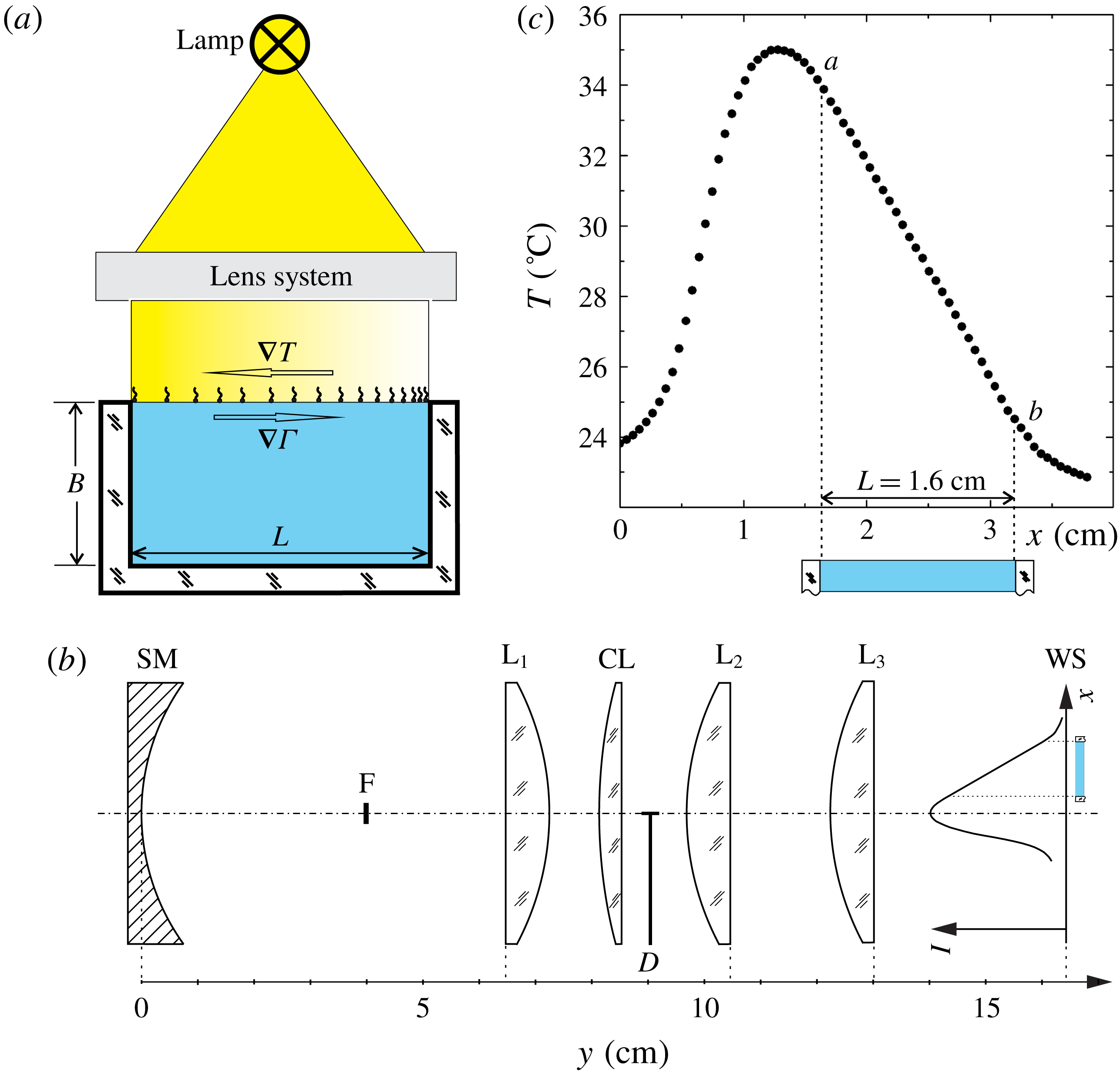
The experiments were carried out in a vertical Hele-Shaw cell formed by two glass plates separated by a glass spacer of 0.25 cm thickness (figure 1
a). The width
 $L$
and depth
 $B$
of the cavity were 1.6 cm and 0.8 cm, respectively. Due to the U-shaped form of the spacer, the upper boundary of the liquid filling the cell remained free. The parts forming the cell were thoroughly washed and rinsed with high-purity water and after drying tightly pressed each to other without glue to minimize the potential sources of contamination. The cell was filled with high-purity water. To avoid the meniscus zone effects, the cell was filled up to the level of the upper edges of the side walls so that the free surface was flat. Before each experiment, the water surface in the cell was additionally cleaned, similar to the procedure used in the Langmuir trough system. The cell was overfilled and the excess liquid was pumped out from the surface by an aspirator together with residual impurities.
(a) General scheme of the experiment. The temperature distribution along the interface is due to absorption of a non-uniform light flux which is created using a lamp and an optical system. Partial contamination of the interface is due to insoluble surfactant. (b) Detailed scheme of the optical system: SM – spherical mirror (
 $f=2$
cm), F – lamp’s filament,
 $\text{L}_{1}$
,
 $\text{L}_{2}$
,
 $\text{L}_{3}$
– three identical spherical lenses (
 $f=8$
cm), CL – cylindrical lens (
 $f=9$
cm), D – half-plane diaphragm, WS – water surface plane. The distribution of the light intensity incident on the surface is shown schematically. (c) The temperature distribution created on motionless surface due to absorption of the non-uniform light flux formed by the optical scheme. The section
 $a$
–
 $b$
with a linear temperature profile was projected onto the water surface to create a constant temperature gradient at the surface of the liquid.

The linear temperature distribution on the free surface was created due to absorption of the non-uniform light flux directed normally to the liquid surface from the side of the gas phase. Such a means of setting the temperature boundary conditions at the free surface has several advantages over the conventionally used scheme when the temperature is fixed at the edges of the surface. In the latter case the temperature profile along the free surface turns out to be highly nonlinear. Almost the entire temperature drop is concentrated in very narrow regions adjacent to the hot and cold walls, while a very small temperature gradient remains on the main part of the interface. In this case, the estimation of the similarity parameters from the experimental data is complicated by the ambiguous nature of the choice of the characteristic temperature gradient in the problem. This makes it difficult to interpret the results of the experiment and compare it with theoretical studies, where the temperature gradient is assumed to be constant along the entire surface of the liquid. The method used by us makes it possible to ensure that the temperature profile remains linear along the surface, which corresponds to the problem statement in theoretical works. In addition, such a method provides an inertialess heat source. The changes in the heat flux and, consequently, in the surface temperature occur on a characteristic time of the order of tenths of a second.
As a light source, we used a halogen lamp with a rectangle filament of size
 $0.3\times 0.4$
cm. The maxima in the emission spectrum of the lamp and in the absorption spectrum of water fall in the near and mid-infrared range, and therefore the main heat release due to the absorbed incident radiation occurs in the narrow near-surface region. The optical system consisting of a spherical mirror, three spherical and one cylindrical lens (see figure 1
b) formed a strongly elongated filament image in the water surface plane. The temperature distribution created on the motionless surface due to absorption of the non-uniform light flux formed by the optical scheme is shown in figure 1(c). In this case the surface was covered by a surfactant layer of surface concentration close to that of a saturated monolayer, which eliminated its mobility. The part of the light flux located in between points
 $a$
and
 $b$
of length 1.6 cm provides a linear temperature distribution. To organize a constant temperature gradient along the water surface in the experimental cell we projected only the
 $a$
–
 $b$
part of the light flux on the water surface (see the schematic drawing of the cell in figure 1
c), while the rest of the light flux passes by the cell and is not used in the experiments. Preliminary experiments showed the presence of small deviations from the linear distribution near the side walls, which are due to the difference in the thermal conductivities of the liquid and wall material and the change of the flow direction at the cell corners. The close thermal conductivities of water and glass and the small thickness of the side walls make the contribution of the first mechanism minimal. This is also confirmed by the fact that the distortions in the temperature profile sharply decrease with decreasing flow velocity in the cell. The largest deviations were observed at the clean water surface, when intensive thermocapillary convection developed on the entire interface. However, even in this case, the region with a nonlinear temperature distribution occupied no more than 5–7 % of the entire length of the liquid surface, which makes it possible to consider the contribution of these sections of the profile as insignificant. The lamp was supplied from an adjustable constant current source, which enabled us to vary, in a wide range intensity, the light flux emitted, changing thereby the slope of the temperature profile in the
 $a$
–
 $b$
part projected onto the interface. The maximum temperature drop achieved on the immobile water surface under the maximum lamp power was 12 K.
An FLIR SC5000 video camera with a matrix sensitive in the infrared range (2.5–
 $5.0~\unicode[STIX]{x03BC}\text{m}$
, matrix resolution
 $320\times 256$
pixels, sensitivity 20 mK) was used to measure the temperature at the free surface. The spatial resolution of the image was
 $0.02~\text{cm}~\text{pix}^{-1}$
. Since the Lambert adsorption coefficient of water within the sensitivity range of the camera matrix is of the order of
 $10^{3}~\text{cm}^{-1}$
(Palmer & Williams Reference Palmer and Williams1974; Downing & Williams Reference Downing and Williams1975), the camera measures the temperature within a narrow near-surface layer of thickness of the order of
 $10~\unicode[STIX]{x03BC}\text{m}$
. The video image was transferred to a PC, where it was processed using the standard FLIR software, which allows us to obtain temporal and spatial distributions of both differential and integral temperature characteristics. In particular, the total temperature difference
 $\unicode[STIX]{x0394}T$
, measured by the camera between the leftmost and rightmost edges, was used to calculate the total surface tension difference caused by the thermocapillary mechanism
 $\unicode[STIX]{x0394}\unicode[STIX]{x1D70E}_{T}=\unicode[STIX]{x1D70E}_{T}\unicode[STIX]{x0394}T$
, where
 $\unicode[STIX]{x1D70E}_{T}=\unicode[STIX]{x2202}\unicode[STIX]{x1D70E}/\unicode[STIX]{x2202}T=0.16~\text{mN}~\text{m}^{-1}~\text{K}^{-1}$
is the temperature coefficient of water surface tension.
A small number of light-scattering particles, namely silver-coated hollow glass spheres (Dantec) with average diameter of
 $15~\unicode[STIX]{x03BC}\text{m}$
, was added to the liquid to visualize the structure of the convective flow in the cell. A wide distribution of particle density allowed one to separate out the particles with neutral buoyancy. Before use, the selected particles underwent a multi-stage cleaning procedure, involving consecutive washing in acetone, isopropanol and high-purity water, to prevent uncontrolled impurities from entering the water. The middle longitudinal plane of the cell was illuminated by a thin light sheet of thickness 0.02 cm formed by a laser. The image was recording with a Jai CM 080 GE video camera with a high spatial-temporal resolution (
 $1032\times 778$
pix, 30 f.p.s.) and was transferred to a PC for further processing. To visualize the structure of the flow, the track images were obtained using the DigiFlow software. To register the velocity field, the particle track velocimetry (PTV) method was applied.
Oleic acid (Merck) was used as a surfactant. It is insoluble in water and has a relatively simple form of surface pressure isotherm, i.e. the dependence of surface pressure
 $\unicode[STIX]{x03C0}$
on the relative surface concentration
 $\unicode[STIX]{x1D6E4}/\unicode[STIX]{x1D6E4}_{e}$
at a fixed temperature, where
 $\unicode[STIX]{x1D6E4}_{e}=7.2\times 10^{-10}~\text{mol}~\text{cm}^{-2}$
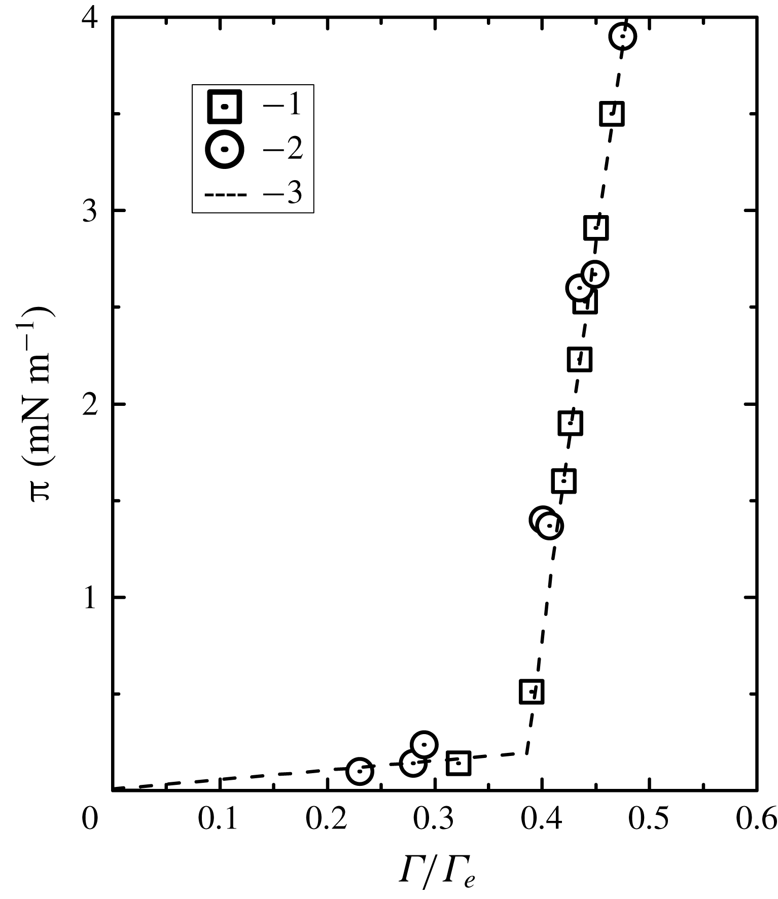
is the surface concentration corresponding to the saturated monolayer (Abramzon & Gaevoy Reference Abramzon and Gaevoy1979). Figure 2 provides the surface pressure isotherm of oleic acid in the concentration range of interest, which is presented both by the data measured by us with the Wilhelmy plate method in a Langmuir trough (Minimicro KSV Ltd., Finland) and as well by those found in the literature (Abramzon & Gaevoy Reference Abramzon and Gaevoy1979). The dependence consists of two linear sections which correspond to different phase states in the layer (Adam Reference Adam1952; Adamson & Gast Reference Adamson and Gast1967). The initial part of the dependence relating to the concentration range
 $\unicode[STIX]{x1D6E4}/\unicode[STIX]{x1D6E4}_{e}<0.38$
and characterized by high compressibility
 $\text{d}\unicode[STIX]{x03C0}/\text{d}(\unicode[STIX]{x1D6E4}/\unicode[STIX]{x1D6E4}_{e})$
describes the layer in the gaseous phase state. Under higher concentration
 $\unicode[STIX]{x1D6E4}/\unicode[STIX]{x1D6E4}_{e}>0.38$
the oleic acid molecules form a layer with a liquid-expanded phase state having much lower compressibility. It has been mentioned above that the maximum temperature difference created on the motionless liquid surface by the lamp and the optical system is 12 K, which corresponds to a maximum surface tension difference due to the thermocapillary mechanism attainable in the experiments of
 $\unicode[STIX]{x0394}\unicode[STIX]{x1D70E}_{T}\approx 2~\text{mN}~\text{m}^{-1}$
. This is sufficient to manipulate the surfactant layers with surface concentration
 $\unicode[STIX]{x1D6E4}/\unicode[STIX]{x1D6E4}_{e}<0.42$
, i.e. within the whole gaseous state and at the beginning of the liquid-expanded state.
Surface pressure
 $\unicode[STIX]{x03C0}$
for oleic acid layer as a function of the relative surface concentration
 $\unicode[STIX]{x1D6E4}/\unicode[STIX]{x1D6E4}_{e}$
(
 $\unicode[STIX]{x1D6E4}_{e}$
stands for the saturated monolayer concentration) measured at
 $20\,^{\circ }\text{C}$
. The symbols indicate: 1 – experimental data obtained in this study, 2 – the data taken from the handbook Abramzon & Gaevoy (Reference Abramzon and Gaevoy1979). Dotted line present a piecewise linear approximation of the data.

Oleic acid was preliminary dissolved in
 $n$
-hexane in the volume ratio of 1 : 70 000. A small amount (few microlitres) of the solution was deposited on the previously cleaned surface of the water. After complete evaporation of the
 $n$
-hexane, a layer of oleic acid molecules with a given surface concentration remained at the interface. The exact value of the solution concentration was determined immediately before the experiment in the Langmuir trough. For this purpose, a certain amount of solution was applied to the cleaned surface of the water subphase and, after evaporation of the hexane, the surface phase was compressed by barriers. The surface pressure was measured using a Wilhelmy plate. If the measured isotherm was displaced relative to the calculated concentration, the initial concentration was adjusted. The purity of the solvent used was tested separately, for which pure
 $n$
-hexane was applied to the cleaned surface of the water filling the Langmuir trough. After complete
 $n$
-hexane evaporation, the surface was compressed by a barrier system, and the surface tension was measured by a Wilhelmy plate. The measurements showed no change in the surface tension at the end of the compression cycle, which indicates the absence of impurities, at least surface-active ones, in the
 $n$
-hexane used.
The experiments were carried out at a temperature of
 $23\,^{\circ }\text{C}$
. It should be noted that with an increase in the applied temperature gradient, the average temperature of the surface slightly increased during the tests and could exceed the temperature in the liquid volume by an average of 3–5 K.
2.2 Experimental results
2.2.1 Overview of the flow structure for different degrees of the surface contamination
Observations have shown that the structure of the convective flow depends substantially both on the applied temperature difference
 $\unicode[STIX]{x0394}T$
and on the initial surface density of the surfactant
 $\unicode[STIX]{x1D6E4}_{0}$
.
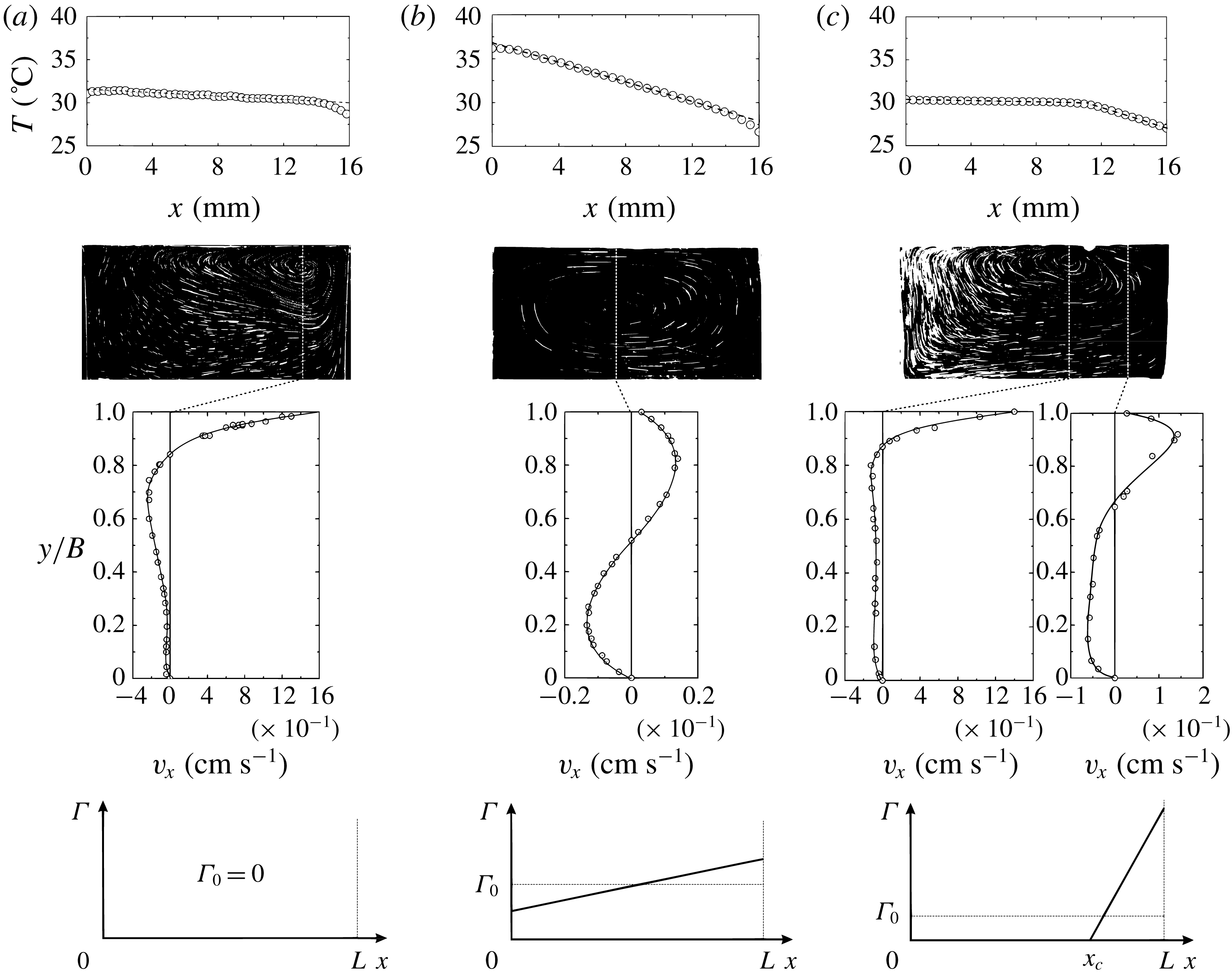
Temperature profile along the interface (upper row), flow structure (second row), vertical profile of the horizontal fluid velocity (third row) and schematic of surface concentration profile of the surfactant (bottom row) for three cases: (a) water surface free of surfactant molecules, i.e.
 $\unicode[STIX]{x1D6E4}_{0}=0$
, (b) strongly contaminated water surface (
 $\unicode[STIX]{x1D6E4}_{0}=0.6$
) when stagnant zone extends to the entire interface, (c) two-zone flow structure,
 $\unicode[STIX]{x1D6E4}_{0}=0.1$
.

In the case of a water surface free of surfactant molecules, i.e. when
 $\unicode[STIX]{x1D6E4}_{0}=0$
, intensive thermocapillary convection develops on the entire interface (see figure 3
a). The velocity profile across the liquid layer, presented in figure 3(a), is typical for the situation under consideration and was observed in previous studies (Birikh Reference Birikh1966; Sen & Davis Reference Sen and Davis1982; Kirdyashkin Reference Kirdyashkin1984; Lappa Reference Lappa2009; Vinnichenko et al.
Reference Vinnichenko, Pushtaev, Plaksina, Rudenko and Uvarov2018). One of the maxima is located at the surface where the velocity is of the order of
 $10^{0}~\text{cm}~\text{s}^{-1}$
. This agrees with the values measured in earlier studies (Kirdyashkin Reference Kirdyashkin1984) at comparable Marangoni number, which is
 $Ma=\unicode[STIX]{x1D70E}_{T}\unicode[STIX]{x0394}TB^{2}/\unicode[STIX]{x1D702}\unicode[STIX]{x1D712}L\cong 0.65\times 10^{4}$
in the situation presented in figure 3(a) (here
 $\unicode[STIX]{x1D702}$
and
 $\unicode[STIX]{x1D712}$
are the viscosity and thermal diffusivity of water, respectively). It is worth noting the position of the vortex centre nearer the cold edge in contrast to another studies where it is located closer to the hot edge (Wanschura et al.
Reference Wanschura, Shevtsova, Kuhlmann and Rath1995; Masud, Kamotani & Ostrach Reference Masud, Kamotani and Ostrach1997; Sim & Zebib Reference Sim and Zebib2002; Kawamura, Tagaya & Hoshino Reference Kawamura, Tagaya and Hoshino2007; Bach & Schwabe Reference Bach and Schwabe2015). The discrepancies are connected to different temperature boundary conditions at the interface. In most studies the temperature is set at the side walls bounding the liquid surface. In this case the main temperature change is concentrated within boundary layers adjacent to the hot and cold walls, while the temperature gradient in the central part of the interface is rather small. Under these conditions the centre of the convective vortex is formed near the hot edge where the maximum in the surface velocity takes place. In the case considered in this paper a permanent thermocapillary force acting along the interface results in the liquid element moving with constant acceleration, acquiring the maximum velocity closer to the cold edge, which defines the location of the vortex centre there. The temperature distribution on the clean water surface (see figure 3
a, upper frame) is linear with small deviations near the walls associated with the change of the flow direction at the cell corners. The temperature profile slope is small owing to the essential contribution of the convective heat transfer mechanism.
When the water surface is heavily contaminated (see figure 3
b), the solutocapillary mechanism always balances the thermocapillary one on the entire surface, which results in formation of a stagnant zone all over the interface. The balance of shearing stresses at the interface, however, does not mean complete surface immobility. The sluggish thermocapillary motion with velocity, of the order of
 $10^{-4}{-}10^{-2}~\text{cm}~\text{s}^{-1}$
, is always present at the interface (see the velocity profile in figure 3
b). This is caused by continuous blurring of the non-uniform distribution of the surfactant by the surface diffusion mechanism, which should be all the time compensated by the thermocapillary flow restoring it. A weak convective flow develops as well in the volume owing to the thermogravitational mechanism of convection. A symmetric convective vortex develops throughout the cell (see figure 3
b). A linear temperature distribution is observed at the interface. It is seen that the temperature profile slope is much greater in comparison with that observed at a clean surface, which results from essential reduction of the convective heat transfer.
The most interesting situation is observed when the surface concentration is so small that the solutocapillary stress cannot balance the thermocapillary one all over the interface. As a result a zone free of surfactant appears near the hot edge (figure 3 c), where an intensive thermocapillary convection develops (figure 3 c). All surfactant turns out to be completely concentrated close to the cold edge, forming a stagnant zone, within of which both surface mechanisms balance each other, which results in the establishing of extremely slow motion at the interface, as in the case presented in figure 3(b). The velocity profiles measured in the volume below free and stagnant zones are similar to those presented in figures 3(a) and 3(b), respectively. The sharp change of the surface velocity by two or three orders of magnitude when passing through a stagnant point leads to a difference in the temperature profiles along the interface inside the zones. The temperature distribution remains linear within each zone but with essentially differing slopes (figure 3 c, upper frame). The characteristic temperature difference is tenths of a degree along the clean zone, while it is equal to several degrees within the stagnant zone. The difference in the temperature profile slopes is due to different heat transfer mechanisms: convective on the clean surface and mainly heat conducting in the region of the stagnant zone. The temperature profile inflection coincides with the position of the stagnant point. Thus, infrared imaging of the surface temperature allows one to visualize a zones location and to measure the position of the stagnation point.
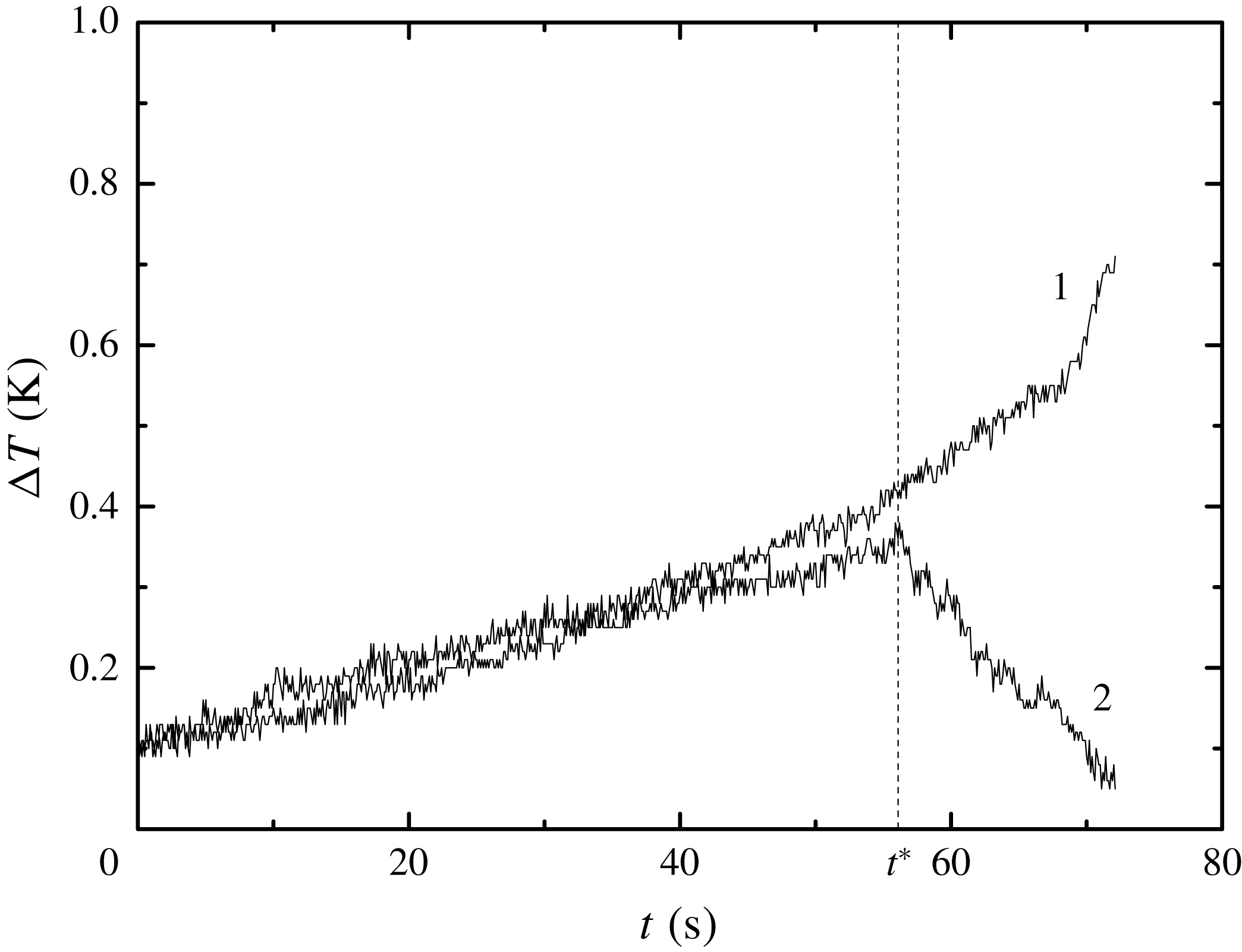
Time dependence of the local temperature difference measured at two surface sections located at the centre of the interface (1) and near the hot edge (2). The temperature gradient applied to the interface are gradually increased with time;
 $t^{\ast }$
is the time when the clean zone appears.

2.2.2 Formation of the two-zone regime
An increase of the temperature gradient applied along a surface comprising a fixed amount of surfactant leads to an increase in the surfactant concentration difference between the surface edges. When the surface concentration of the surfactant on the hot edge of the interface reaches zero a two-zone flow structure arises. The critical temperature difference
 $\unicode[STIX]{x0394}T^{\ast }$
which corresponds to the appearance of a clean surface zone depends on the initial surface concentration
 $\unicode[STIX]{x1D6E4}_{0}$
of the oleic acid. The following experimental procedure was applied to measure
 $\unicode[STIX]{x0394}T^{\ast }$
. At a certain initial surfactant concentration the light intensity was increased slowly with time from zero to a maximum, which resulted in a gradual increase of the total temperature difference over entire surface. To define the moment when the clean zone appears we compared the local temperature differences measured at two 2 mm length surface sections located near the hot edge and at the centre of the interface as a function of time. An example of such dependence is presented in figure 4. It is seen that, at the beginning, when the total temperature difference is still small, the local temperature differences are the same, which indicates a constant temperature gradient over entire interface as in figure 3(b) (upper frame). Later on, as the applied temperature gradient increases, the local temperature difference measured near the hot edge begins to decrease abruptly while that at the centre it continues to grow, which means there is the formation of a clean zone and appearance of an inflection on the temperature profile, as in figure 3(c) (upper frame). The total temperature difference, measured at time
 $t^{\ast }$
, beginning when the local temperature differences start to be unequal, is the required critical temperature difference
 $\unicode[STIX]{x0394}T^{\ast }$
.
It is found that
 $\unicode[STIX]{x0394}T^{\ast }$
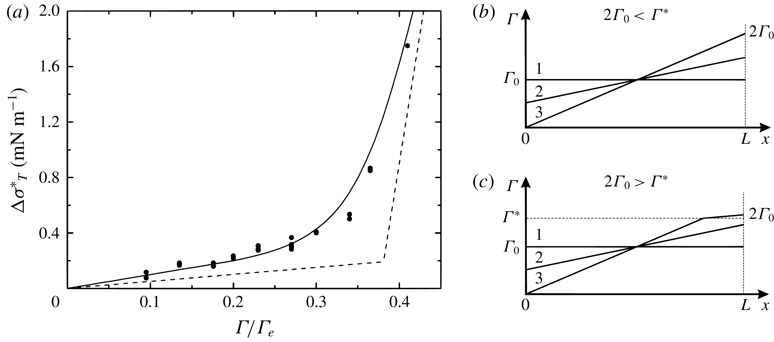
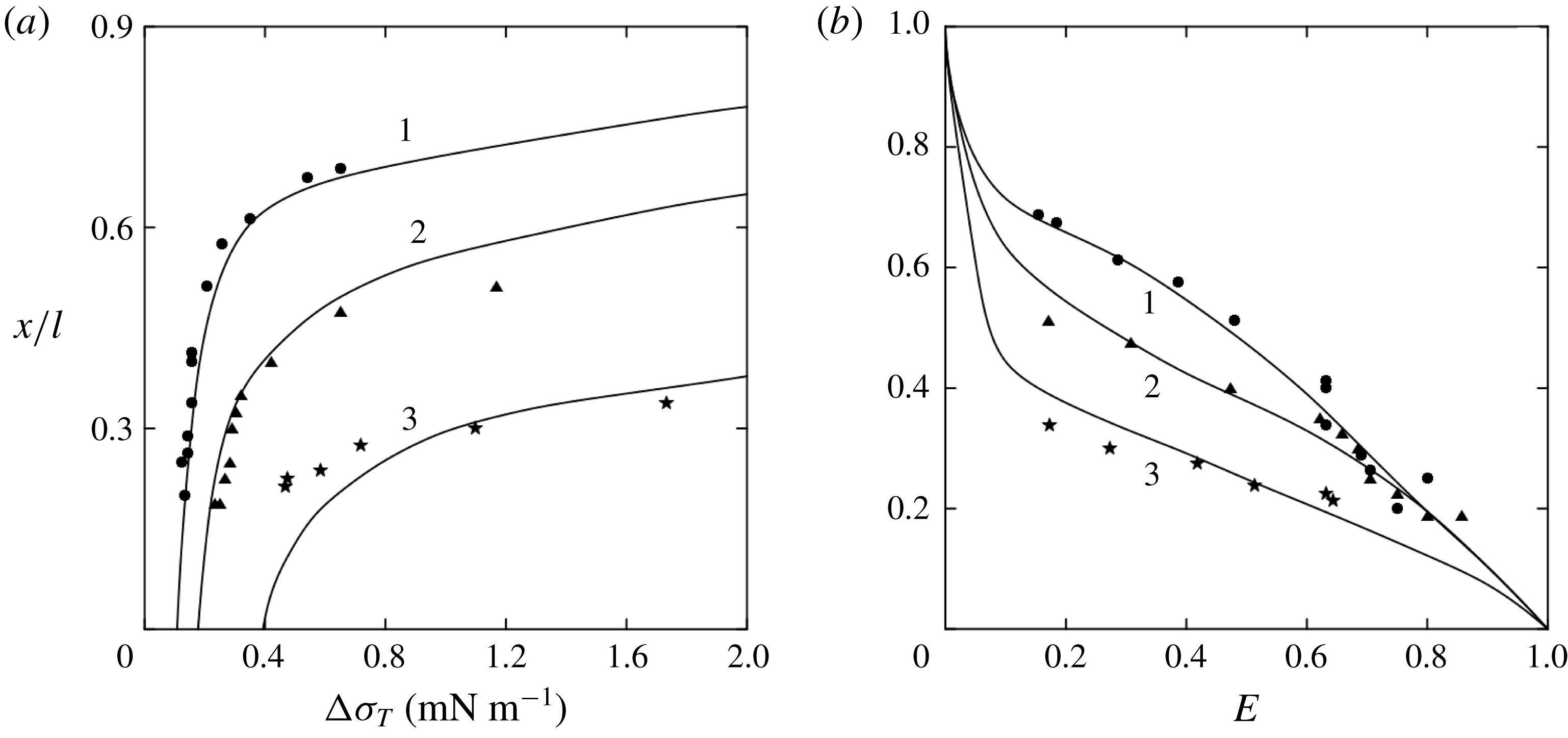
essentially depends on the initial surfactant concentration. The more surfactant was added to the surface at the beginning of the experiment, the higher the temperature difference necessary for the appearance of the clean zone. Figure 5(a) shows the value of the critical increment of the surface tension
 $\unicode[STIX]{x0394}\unicode[STIX]{x1D70E}_{T}^{\ast }=\unicode[STIX]{x1D70E}_{T}\unicode[STIX]{x0394}T^{\ast }$
due to the thermocapillary mechanism as a function of the initial surfactant concentration
 $\unicode[STIX]{x1D6E4}_{0}/\unicode[STIX]{x1D6E4}_{e}$
. In the same plot the isotherm of oleic acid, as in figure 2, is given schematically for comparison. It is seen that the dependencies are similar, but they do not coincide. At first glance, this fact seems strange, since both dependencies reflect the growth of the applied shear stress holding the layer as the surfactant concentration increases. However, in reality, there are significant differences between them. The isotherm is obtained by measuring the surface pressure in the surfactant layer whose concentration is uniform everywhere. Under laboratory conditions, this dependence is usually obtained in a Langmuir trough. The surfactant layer is compressed by a movable barrier, and the surface pressure is measured with a Wilhelmy plate at various concentrations. Then, the surface pressure
 $\unicode[STIX]{x03C0}$
is applied along the contact line of the barrier with the interface, and the surfactant concentration is always constant throughout the interface, being almost instantaneously equalized when the position of the barrier is changed.
(a) Dependence of
 $\unicode[STIX]{x0394}\unicode[STIX]{x1D70E}_{T}^{\ast }$
on the initial concentration of oleic acid
 $\unicode[STIX]{x1D6E4}_{0}/\unicode[STIX]{x1D6E4}_{e}$
. The surface pressure isotherm for oleic acid
 $\unicode[STIX]{x03C0}=f(\unicode[STIX]{x1D6E4}_{0}/\unicode[STIX]{x1D6E4}_{e})$
(dotted line) is presented schematically for comparison. The curve calculated from (2.4) is shown with a solid line. Schematic presentation of the surfactant distribution along the interface as the temperature gradient along the interface rises for the cases when the layer remains in gaseous phase state (b) and when the part of the surfactant located near the cold edge is in liquid-expanded phase state (c). The curves in (b) and (c) correspond to the cases: 1, initial surfactant distribution in absence of the heating; 2, temperature gradient is small enough to provide a clean zone appearance; 3, surfactant distribution under appearance of a clean zone.

Quite a different situation is observed in the case being considered in this paper. The presence of the constant temperature gradient along the interface causes the appearance of a tangential stress, thermocapillary in nature, which is constant at each point. This in turn results in the formation of a constant gradient of surfactant concentration and, therefore, additional tangential stress, solutocapillary in nature, the interface. To achieve a stress balance on the surface, the surface tension increment due to uneven heating
 $\unicode[STIX]{x0394}\unicode[STIX]{x1D70E}_{T}$
should to be equal to that caused by the uneven surfactant distribution
 $\unicode[STIX]{x0394}\unicode[STIX]{x1D70E}_{\unicode[STIX]{x1D6E4}}$
. As is seen from the scheme in figure 5(b), the latter can be found as
 $\unicode[STIX]{x0394}\unicode[STIX]{x1D70E}_{\unicode[STIX]{x1D6E4}}=2\unicode[STIX]{x1D70E}_{\unicode[STIX]{x1D6E4}}\unicode[STIX]{x1D6E4}_{0}$
, where
 $\unicode[STIX]{x1D70E}_{\unicode[STIX]{x1D6E4}}$
is the concentration coefficient of the water surface tension in the gaseous phase. Note that this is twice as much as the surface pressure necessary for the stress balance in the case of a layer with constant concentration. This is why the dependence
 $\unicode[STIX]{x0394}\unicode[STIX]{x1D70E}_{T}^{\ast }(\unicode[STIX]{x1D6E4}_{0}/\unicode[STIX]{x1D6E4}_{e})$
has a slope which is twice that of the isotherm in the range of small values of surface concentration. Another difference between these dependencies is associated with the different scenarios of phase transition in the surfactant layer. In the case of compression of the latter by the barrier, the entire layer is completely transferred from the gaseous state to the liquid-expanded state upon reaching the critical concentration
 $\unicode[STIX]{x1D6E4}^{\ast }=0.38\unicode[STIX]{x1D6E4}_{e}$
. This is why the isotherm obtained in a barrier system looks like two linear sections corresponding to different phase states, with a rather sharp transition between them.
In the thermocapillary case, if
 $2\unicode[STIX]{x1D6E4}_{0}>\unicode[STIX]{x1D6E4}^{\ast }$
, the part of the surfactant layer located near the cold edge of the surface transits to a liquid-expanded phase state (see figure 5
c) when the clean zone arises near the hot edge. At that, the remaining part of the layer is still in the gaseous phase state. Thus, a situation unusual for physical chemistry is established at the interface, when different parts of the surfactant layer are simultaneously in different phase states, which are characterized by different compressibilities. The surface tension increment due to solutocapillary mechanism consists in this case of two parts
 $\unicode[STIX]{x0394}\unicode[STIX]{x1D70E}_{\unicode[STIX]{x1D6E4}}=\unicode[STIX]{x0394}\unicode[STIX]{x1D70E}_{\unicode[STIX]{x1D6E4}}^{g}+\unicode[STIX]{x0394}\unicode[STIX]{x1D70E}_{\unicode[STIX]{x1D6E4}}^{l}=\unicode[STIX]{x1D70E}_{\unicode[STIX]{x1D6E4}}\unicode[STIX]{x1D6E4}^{\ast }+\unicode[STIX]{x1D70E}_{\unicode[STIX]{x1D6E4}}^{l}(\unicode[STIX]{x1D6E4}_{m}-\unicode[STIX]{x1D6E4}^{\ast })$
, where
 $\unicode[STIX]{x0394}\unicode[STIX]{x1D70E}_{\unicode[STIX]{x1D6E4}}^{g}$
and
 $\unicode[STIX]{x0394}\unicode[STIX]{x1D70E}_{\unicode[STIX]{x1D6E4}}^{l}$
are the surface tension increments in the layer parts in gaseous and liquid-extended phase states, respectively,
 $\unicode[STIX]{x1D70E}_{\unicode[STIX]{x1D6E4}}^{l}$
is concentration dependence of surface tension in the liquid-expanded phase state,
 $\unicode[STIX]{x1D6E4}_{m}$
is the surfactant concentration at the cold edge of the interface. As the area occupied by the liquid-expanded section of the layer increases, the slope of the
 $\unicode[STIX]{x0394}\unicode[STIX]{x1D70E}_{T}^{\ast }(\unicode[STIX]{x1D6E4}_{0}/\unicode[STIX]{x1D6E4}_{e})$
dependence gradually increases, approaching the slope of surface pressure isotherm (dotted line) corresponding to the liquid-extended phase state. It should be noted, however, that this slope will never be reached, since a small part of the layer near the hot edge of the interface will always be in the gaseous phase state.
The experimentally obtained dependence
 $\unicode[STIX]{x0394}\unicode[STIX]{x1D70E}_{T}^{\ast }(\unicode[STIX]{x1D6E4}_{0}/\unicode[STIX]{x1D6E4}_{e})$
can be described analytically based on obvious physical considerations and geometrical relations. Firstly, the surface pressure isotherm should be presented as a piecewise function
 $$\begin{eqnarray}\unicode[STIX]{x03C0}=\left\{\begin{array}{@{}ll@{}}\unicode[STIX]{x1D70E}_{\unicode[STIX]{x1D6E4}}\unicode[STIX]{x1D6E4},\quad & \text{if}~\unicode[STIX]{x1D6E4}\leqslant \unicode[STIX]{x1D6E4}^{\ast };\\ \unicode[STIX]{x1D70E}_{\unicode[STIX]{x1D6E4}}\unicode[STIX]{x1D6E4}^{\ast }+\unicode[STIX]{x1D70E}_{\unicode[STIX]{x1D6E4}}^{l}(\unicode[STIX]{x1D6E4}-\unicode[STIX]{x1D6E4}^{\ast }),\quad & \text{if}~\unicode[STIX]{x1D6E4}>\unicode[STIX]{x1D6E4}^{\ast }.\end{array}\right.\end{eqnarray}$$
Secondly, it is necessary to take into account the fact that the gradient of surface tension due to the solutocapillary mechanism should be the same in the gaseous and in the liquid-extended parts of the layer
 $$\begin{eqnarray}\frac{\unicode[STIX]{x1D70E}_{\unicode[STIX]{x1D6E4}}\unicode[STIX]{x1D6E4}^{\ast }}{l}=\frac{\unicode[STIX]{x1D70E}_{\unicode[STIX]{x1D6E4}}^{l}(\unicode[STIX]{x1D6E4}-\unicode[STIX]{x1D6E4}^{\ast })}{L-l},\end{eqnarray}$$
where
 $l$
is the size of the surface occupied by the gaseous phase. It is also necessary to allow for the conservation law of the surfactant amount at the interface
 $$\begin{eqnarray}\unicode[STIX]{x1D6E4}_{0}L=\int _{0}^{L}\unicode[STIX]{x1D6E4}\,\text{d}x=\unicode[STIX]{x1D6E4}^{\ast }\frac{l}{2}+(\unicode[STIX]{x1D6E4}^{\ast }+\unicode[STIX]{x1D6E4}_{m})\frac{L-l}{2}.\end{eqnarray}$$
Solving the set of (2.1)–(2.3), one can obtain the following expression for the critical increment of surface tension due to the thermocapillary mechanism:
 $$\begin{eqnarray}\unicode[STIX]{x0394}\unicode[STIX]{x1D70E}_{T}^{\ast }=\left\{\begin{array}{@{}ll@{}}2\unicode[STIX]{x1D70E}_{\unicode[STIX]{x1D6E4}}\unicode[STIX]{x1D6E4}_{0},\quad & \text{if}~2\unicode[STIX]{x1D6E4}_{0}\leqslant \unicode[STIX]{x1D6E4}^{\ast };\\ \unicode[STIX]{x1D70E}_{\unicode[STIX]{x1D6E4}}\unicode[STIX]{x1D6E4}^{\ast }+\unicode[STIX]{x1D70E}_{\unicode[STIX]{x1D6E4}}^{l}(\unicode[STIX]{x1D6E4}_{m}-\unicode[STIX]{x1D6E4}^{\ast }),\quad & \text{if}~2\unicode[STIX]{x1D6E4}_{0}>\unicode[STIX]{x1D6E4}^{\ast },\end{array}\right.\end{eqnarray}$$
where
 $$\begin{eqnarray}\unicode[STIX]{x1D6E4}_{m}=\unicode[STIX]{x1D6E4}_{0}+\sqrt{{\unicode[STIX]{x1D6E4}_{0}}^{2}-\left(1-\frac{\unicode[STIX]{x1D70E}_{\unicode[STIX]{x1D6E4}}}{\unicode[STIX]{x1D70E}_{\unicode[STIX]{x1D6E4}}^{l}}\right)(2\unicode[STIX]{x1D6E4}_{0}-\unicode[STIX]{x1D6E4}^{\ast })\unicode[STIX]{x1D6E4}^{\ast }}.\end{eqnarray}$$
The curve calculated from (2.4) is shown in figure 5(a) with a solid line. It can be seen that the results of the calculation describe well the results of the experiments, which indicates a correct understanding of the physical processes occurring at the interface.
Thus, the two dependencies shown in figure 5(a) are the surface pressure isotherms measured for the same surfactant but under various conditions. The lower curve is obtained under local action (along a contact line with barrier) on the layer with constant surfactant concentration throughout the interface and single-stage phase transition within the whole layer. Such a type of isotherm is usually given in the literature on the physical chemistry. The upper curve is obtained under a distributed action on the surfactant layer (thermocapillary stress acts in each point of the interface), which results in non-uniform surfactant concentration and makes possible the simultaneous coexistence of different parts of the layer in different phase states.
2.2.3 Measurement of a stagnant point position
As the clean zone appears, the position of the stagnant point, dividing the clean and the stagnant zones, essentially depends on both the applied temperature difference
 $\unicode[STIX]{x0394}T$
and the initial surface concentration of the surfactant
 $\unicode[STIX]{x1D6E4}_{0}$
. Increase in the temperature difference between the surface’s edges results in displacement of the stagnant point in the direction of the cold edge. And vice versa, the stagnant point shifts towards the hot edge under an increase in the initial surface concentration. In the pioneer works of Homsy & Maiburg and Carpenter & Homsy, who were the first to study this problem theoretically, there was suggested a non-dimensional parameter, the elasticity number, reflecting the relative contribution of the solutal and thermal mechanisms to surface tension variations.
To compare the results obtained by us experimentally with their theoretical predictions we plotted the dimensionless position of the stagnant point
 $x_{c}/L$
as a function of elasticity number. The latter was defined in the same way as in Homsy & Meiburg (Reference Homsy and Meiburg1984)
 $$\begin{eqnarray}E=\frac{\unicode[STIX]{x0394}\unicode[STIX]{x1D70E}_{\unicode[STIX]{x1D6E4}}}{\unicode[STIX]{x0394}\unicode[STIX]{x1D70E}_{T}}=\frac{2\unicode[STIX]{x1D70E}_{\unicode[STIX]{x1D6E4}}\unicode[STIX]{x1D6E4}_{0}}{\unicode[STIX]{x1D70E}_{T}\unicode[STIX]{x0394}T}.\end{eqnarray}$$
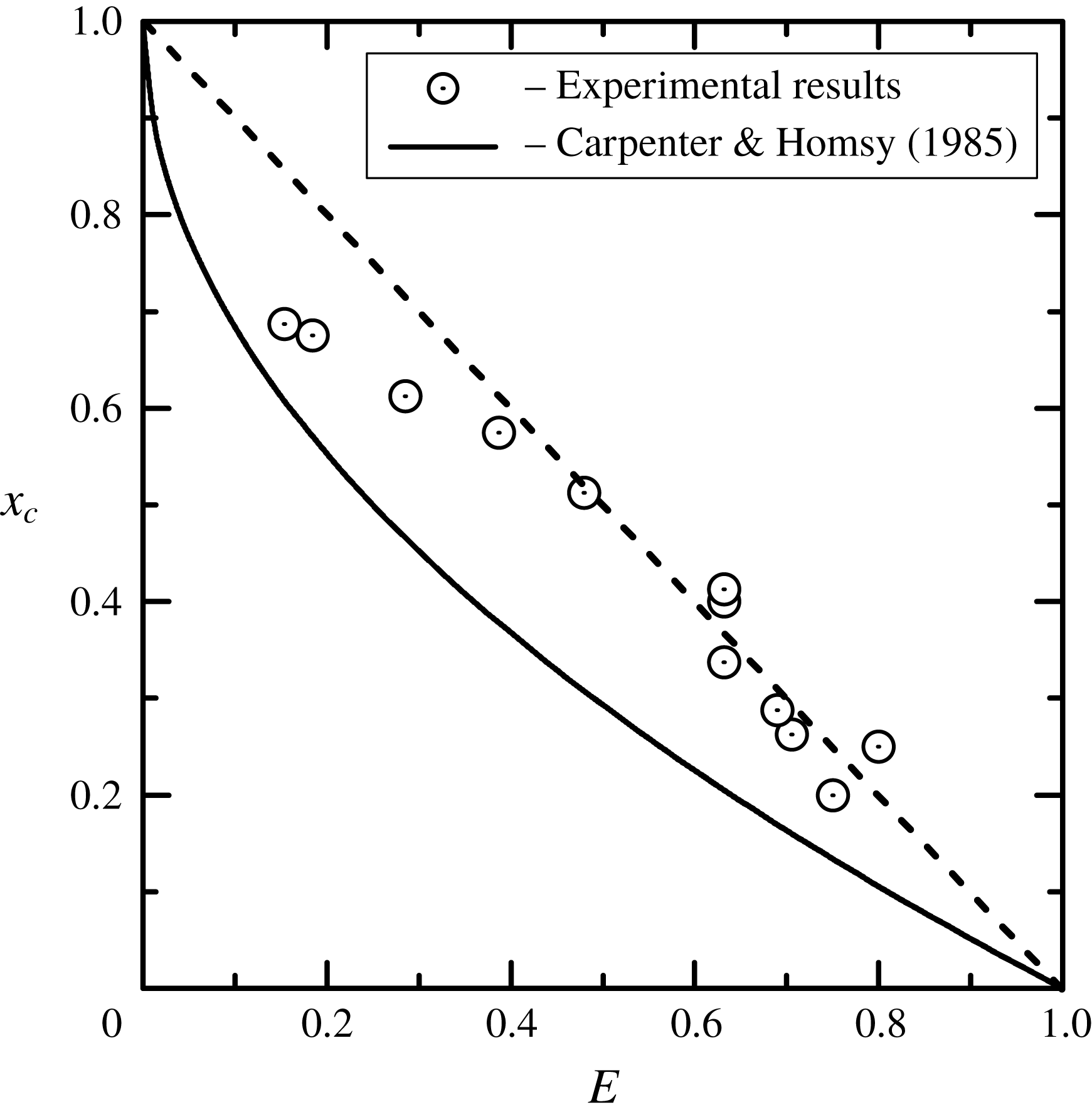
Figure 6 presents such a dependence for the initial surface concentration of the oleic acid
 $\unicode[STIX]{x1D6E4}_{0}/\unicode[STIX]{x1D6E4}_{e}=0.1$
. It can be seen that in the region of large values of the elasticity number
 $0.5<E<1$
the experimental points lie on the bisectrix
 $x_{c}/L=1-E$
(dotted line), forming a linear relationship. However, in the region
 $E<0.5$
, which corresponds to
 $x_{c}<0.5$
, the dependence becomes nonlinear, the free zone begins to grow more slowly with a decrease in the elasticity number, which indicates a worse compressibility. The position of the stagnant point
 $x_{c}=0.5$
represents the situation when the part of the interface occupied by the surfactant decreased twice in comparison with the initial one. Under these conditions the surfactant concentration at the cold edge becomes
 $\unicode[STIX]{x1D6E4}_{m}=0.4\unicode[STIX]{x1D6E4}_{e}$
, i.e. the part of the layer being in liquid-expanded phase state appears. The associated worsening in the compressibility of the layer leads to a deviation from the linear dependence.
Dimensionless position of the stagnant zone
 $x_{c}/L$
as a function of the elasticity number
 $E$
for the initial surfactant concentration
 $\unicode[STIX]{x1D6E4}_{0}/\unicode[STIX]{x1D6E4}_{e}=0.1$
. Open circles correspond to the experiments with oleic acid. Dotted line is the bisectrix
 $x_{c}/L=1-E$
. The solid line represents the analytical result by Carpenter & Homsy (Reference Carpenter and Homsy1985) obtained for simple one-phase surfactant layer within a lubrication approximation.

The solid line shown in figure 6 presents the result of a theoretical study (Carpenter & Homsy Reference Carpenter and Homsy1985) which is described by the equation
 $x_{c}/L=1-\sqrt{E}$
. Before we compare, it is worth taking into account that this dependence was obtained under the assumption of a linear equation of state for the surfactant, which corresponds to the gaseous state of the layer. It can be seen that the theoretical dependence is far from a correct description of the experimental data even in the region where the entire surfactant layer remained in the gaseous state upon compression (the first seven experimental points in the lower right quarter). The discrepancies, in our opinion, are associated with incorrect estimation of the contribution of convective and heat-conductive mechanisms into heat transfer processes. Using the lubrication approximation, the authors neglected the weak, in their opinion, convective heat transfer, leaving the heat conductivity as the only heat transfer mechanism. As a result, the temperature gradient at the interface remains constant even after the appearance of a surfactant-free region. The experimental results presented above clearly demonstrate the presence of inflection in the temperature profile after the free zone appears, which is certainly caused by the significant contribution of thermocapillary convection to heat transfer. Thus the theoretical model needs to be improved by taking into account new experimental observations and should be extended for a description of a possible phase transition in the layer.
3 Asymptotic theory
3.1 Mathematical formulation
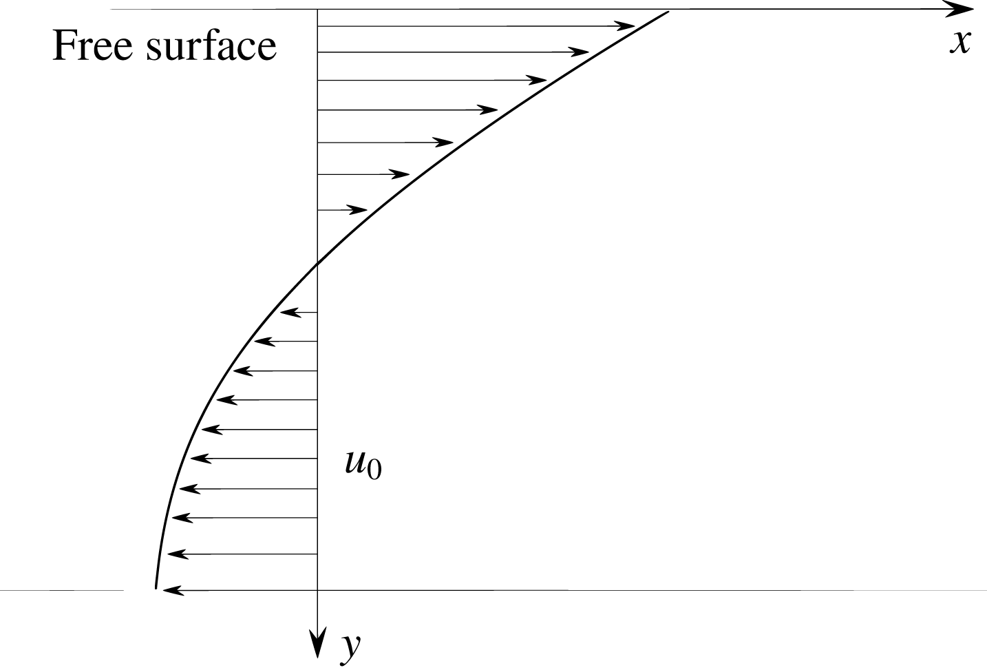
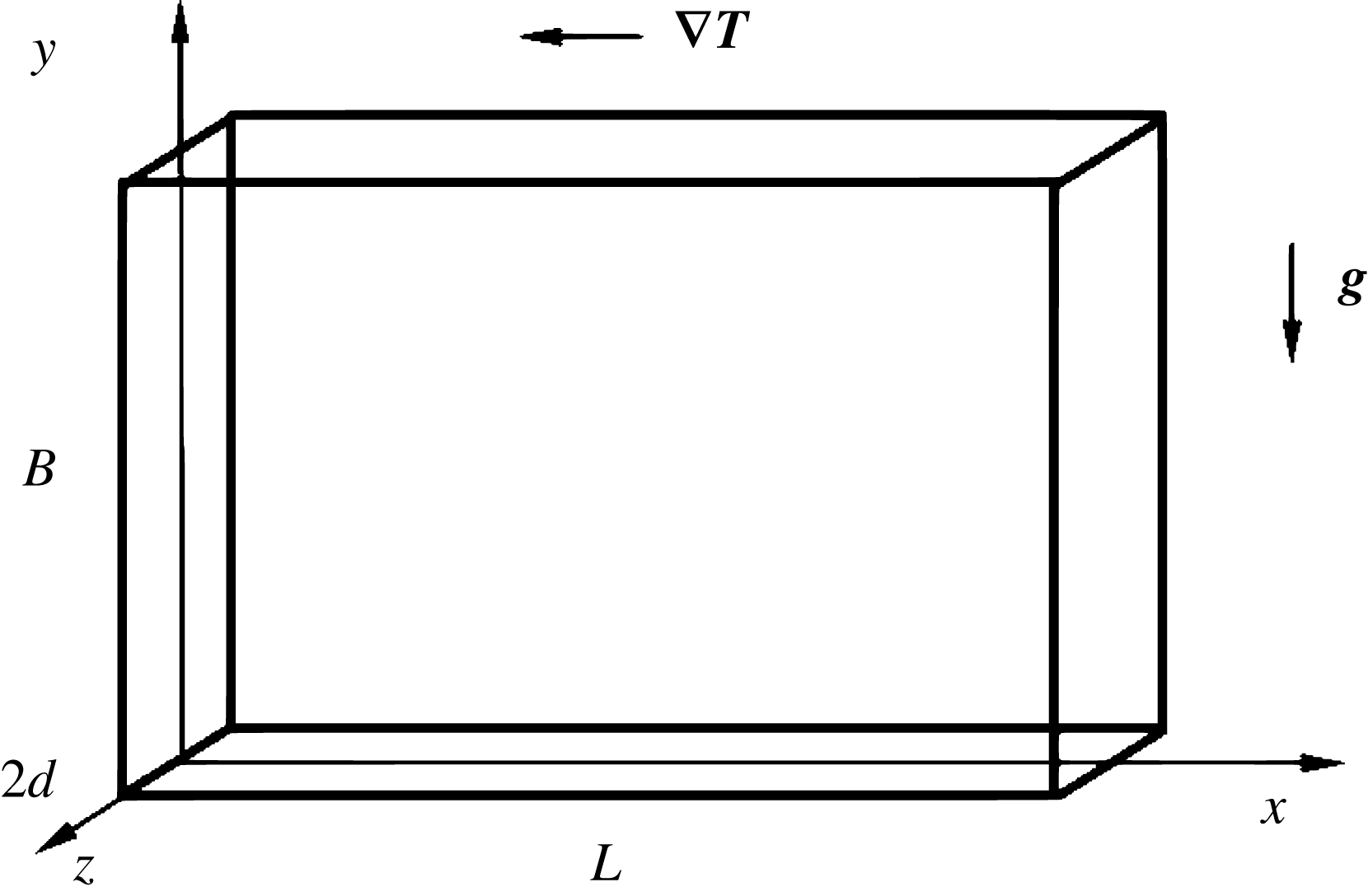
Let us consider a rectangular cavity of length
 $L$
and height
 $B$
. In order to exploit the disparity between two length scales and to apply the theory of lubrication, we consider a thin boundary layer adjacent to the surface with a thickness of
 $\hat{B}$
so that the ratio
 $\unicode[STIX]{x1D700}=\hat{B}/L$
is small (figure 7). We introduce a Cartesian coordinate system, as shown in the figure. The cavity is filled by an incompressible Newtonian liquid with constant physical properties: density
 $\unicode[STIX]{x1D70C}$
, thermal diffusivity
 $\unicode[STIX]{x1D712}$
and dynamic viscosity
 $\unicode[STIX]{x1D702}$
. The temperature gradient across the cavity is maintained by employing a fixed temperature difference
 $\unicode[STIX]{x1D6E9}=T_{1}-T_{2}$
, where
 $T_{1}$
and
 $T_{2}$
are the temperatures of the solid side walls with
 $T_{1}>T_{2}$
. The bottom of the cavity is thermally insulated. For simplicity, we assume that the bottom of the boundary layer
 $y=0$
has the same properties. Since the presence of the gravitational field for lubrication theory is not essential, we assume here that the system is under a weightlessness condition. We assume also that the upper gas–liquid surface remains flat and undeformable during the entire evolution on the surface, which is motivated by the experimental observations presented above.
The coordinate system used for the lubrication theory and zero-order solution for the velocity of the boundary layer flow in the surfactant-free area.

Let us assume further that the surface tension is a function of both temperature
 $T$
with insoluble surfactant of concentration
 $\unicode[STIX]{x1D6E4}$
at the interface. In addition, we admit the scenario in which the advection induced by the thermocapillary effect can create a critical surfactant concentration resulting in the precipitation of a new, distinct phase. In what follows, we consider three possible scenarios:
(i) surfactant in a one-phase gaseous state;
(ii) surfactant in a two-phase state including gaseous and condensed phases with a possible transition between them; and
(iii) surfactant in a two-phase state including gaseous and liquid-expanded phases with a possible transition between them.
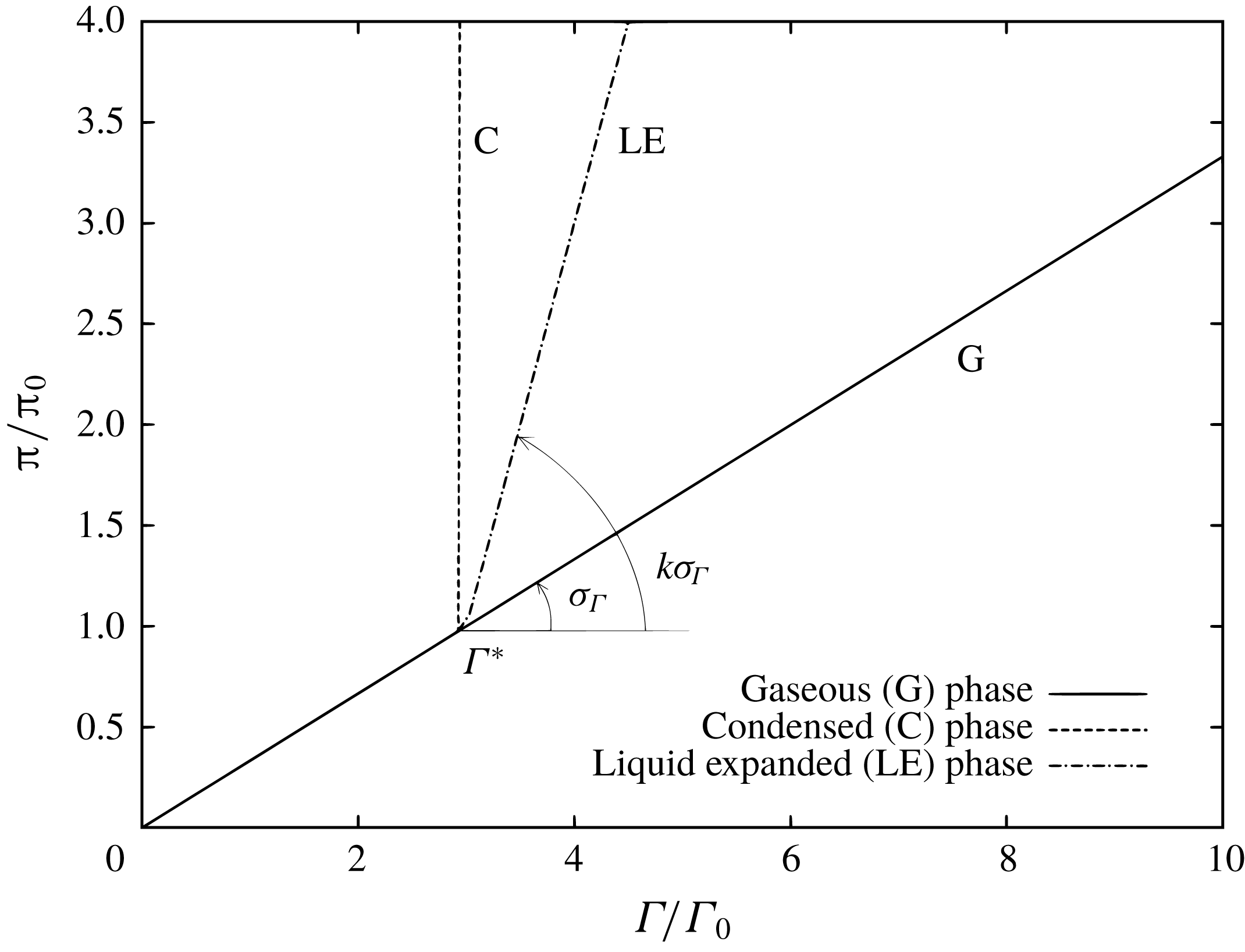
The isotherm of surface pressure
 $\unicode[STIX]{x03C0}$
as a function of the surfactant concentration
 $\unicode[STIX]{x1D6E4}/\unicode[STIX]{x1D6E4}_{0}$
(
 $\unicode[STIX]{x1D6E4}_{0}$
stands for the initial surfactant concentration) is shown in figure 8 for the three possible scenarios (i)–(iii) listed above. As one can see, the critical concentration
 $\unicode[STIX]{x1D6E4}^{\ast }$
occurs when the phase transition from a gaseous state (
 $\unicode[STIX]{x1D6E4}<\unicode[STIX]{x1D6E4}^{\ast }$
) to a condensed or liquid-expanded state (
 $\unicode[STIX]{x1D6E4}>\unicode[STIX]{x1D6E4}^{\ast }$
) takes place. Based on the experimental data obtained for the oleic acid isotherm figure 2, the analytical expression for the surface tension can be written in the following form:
 $$\begin{eqnarray}\unicode[STIX]{x1D70E}=\unicode[STIX]{x1D70E}_{0}-\unicode[STIX]{x1D70E}_{T}T-\unicode[STIX]{x1D70E}_{\unicode[STIX]{x1D6E4}}\boldsymbol{H}(\unicode[STIX]{x1D6E4}^{\ast }-\unicode[STIX]{x1D6E4})\unicode[STIX]{x1D6E4}-k\unicode[STIX]{x1D70E}_{\unicode[STIX]{x1D6E4}}\boldsymbol{H}(\unicode[STIX]{x1D6E4}-\unicode[STIX]{x1D6E4}^{\ast })\left(\unicode[STIX]{x1D6E4}-\unicode[STIX]{x1D6E4}^{\ast }+\frac{1}{k}\unicode[STIX]{x1D6E4}^{\ast }\right),\end{eqnarray}$$
where
 $\unicode[STIX]{x1D70E}_{0}$
is the tension of the clean surface,
 $\unicode[STIX]{x1D70E}_{T}$
is the coefficient of the linear relation between the tension of the clean surface and the temperature,
 $\unicode[STIX]{x1D70E}_{\unicode[STIX]{x1D6E4}}$
is the similar relation between the surface tension and the surfactant concentration in the gaseous phase, the coefficient
 $k$
tunes the linear dependence of the surface tension on the surfactant concentration in the gaseous (
 $k=1$
), liquid-expanded (
 $1<k<\infty$
) and condensed (
 $k\rightarrow \infty$
) phases (see figure 8). In what follows, we assume that the compressibility of the surfactant film in the liquid-expanded state decreases by one order of magnitude with respect to the gaseous phase:
 $k=10$
. Here,
 $\boldsymbol{H}(x)$
stands for the Heaviside step function whose value is 0 for negative argument and 1 for positive argument. Since in this paper many of the dependencies between variables are expressed in the form of a piecewise-defined function, it is convenient to use the Heaviside function.
Schematic presentation of the dimensionless surface pressure as a function of dimensionless surfactant concentration for three possible scenarios of phase transition.

As it is known that the surface tension reduces in the presence of both temperature and surfactant, all the terms in (3.1) are subtracted from
 $\unicode[STIX]{x1D70E}_{0}$
. We assume that the surfactant can form a surface gaseous state for a highly expanded monolayer (when the thermocapillary flow is weak). This state is described by the third term in (3.1). As this state is compressed due to the flow, the surfactant enters the liquid-expanded phase, characterized by the presence of surfactant molecules with their chains in a disordered, liquid-like, phase out of the plane of the interface. This state is described by the last term in (3.1). The scenario is realized, for example, for oleic acid. In some cases, the transition from a gaseous phase to a condensed phase happens without the formation of intermediate states. The condensed phase is characterized by dense packing of surfactant molecules and poor compressibility of the surfactant film. This kind of behaviour can be observed for stearic acid. Most substances, however, show the transition from a gaseous state to a solid-like condensed monolayer state through a sequence of liquid-expanded and liquid-condensed phases.
In order to get an analytic solution for the steady thermocapillary flow in a shallow slot, we apply the theory originally developed for a pure thermocapillary flow by Sen & Davis (Reference Sen and Davis1982) and then extended to the case of the same flow with partially contaminated surface by Carpenter & Homsy (Reference Carpenter and Homsy1985). So, we introduce the lubrication-type scalings: length –
 $L$
, height –
 $\hat{B}$
,
 $x$
-velocity component –
 $\unicode[STIX]{x1D70E}_{T}\unicode[STIX]{x1D6E9}\hat{B}/\unicode[STIX]{x1D702}L$
,
 $y$
-velocity component –
 $\unicode[STIX]{x1D70E}_{T}\unicode[STIX]{x1D6E9}\hat{B}^{2}/\unicode[STIX]{x1D702}L^{2}$
, temperature –
 $\unicode[STIX]{x1D6E9}$
, pressure –
 $\unicode[STIX]{x1D70E}_{T}\unicode[STIX]{x1D6E9}/\hat{B}$
, surfactant concentration –
 $\unicode[STIX]{x1D6E4}_{0}$
, and obtain a set of governing equations which includes the continuity equation, two components of the Navier–Stokes equation and the heat transfer equation, respectively,
 $$\begin{eqnarray}\displaystyle & \displaystyle \frac{\unicode[STIX]{x2202}u}{\unicode[STIX]{x2202}x}+\frac{\unicode[STIX]{x2202}v}{\unicode[STIX]{x2202}y}=0, & \displaystyle\end{eqnarray}$$
 $$\begin{eqnarray}\displaystyle & \displaystyle \unicode[STIX]{x1D700}R\left(u\frac{\unicode[STIX]{x2202}u}{\unicode[STIX]{x2202}x}+v\frac{\unicode[STIX]{x2202}u}{\unicode[STIX]{x2202}y}\right)=-\frac{\unicode[STIX]{x2202}p}{\unicode[STIX]{x2202}x}+\unicode[STIX]{x1D700}^{2}\frac{\unicode[STIX]{x2202}^{2}u}{\unicode[STIX]{x2202}x^{2}}+\frac{\unicode[STIX]{x2202}^{2}u}{\unicode[STIX]{x2202}y^{2}}, & \displaystyle\end{eqnarray}$$
 $$\begin{eqnarray}\displaystyle & \displaystyle \unicode[STIX]{x1D700}^{3}R\left(u\frac{\unicode[STIX]{x2202}v}{\unicode[STIX]{x2202}x}+v\frac{\unicode[STIX]{x2202}v}{\unicode[STIX]{x2202}y}\right)=-\frac{\unicode[STIX]{x2202}p}{\unicode[STIX]{x2202}y}+\unicode[STIX]{x1D700}^{4}\frac{\unicode[STIX]{x2202}^{2}v}{\unicode[STIX]{x2202}x^{2}}+\unicode[STIX]{x1D700}^{2}\frac{\unicode[STIX]{x2202}^{2}v}{\unicode[STIX]{x2202}y^{2}}, & \displaystyle\end{eqnarray}$$
 $$\begin{eqnarray}\displaystyle & \displaystyle \unicode[STIX]{x1D700}M\left(u\frac{\unicode[STIX]{x2202}T}{\unicode[STIX]{x2202}x}+v\frac{\unicode[STIX]{x2202}T}{\unicode[STIX]{x2202}y}\right)=\unicode[STIX]{x1D700}^{2}\frac{\unicode[STIX]{x2202}^{2}T}{\unicode[STIX]{x2202}x^{2}}+\frac{\unicode[STIX]{x2202}^{2}T}{\unicode[STIX]{x2202}y^{2}}, & \displaystyle\end{eqnarray}$$
where
 $u$
and
 $v$
stand for the
 $x$
and
 $y$
components of the fluid velocity. Dimensionless parameters that appear in (3.2)–(3.5)
 $$\begin{eqnarray}R=\frac{\unicode[STIX]{x1D70E}_{T}\unicode[STIX]{x1D6E9}\hat{B}\unicode[STIX]{x1D70C}}{\unicode[STIX]{x1D702}^{2}}\unicode[STIX]{x1D700},\quad M=\frac{\unicode[STIX]{x1D70E}_{T}\unicode[STIX]{x1D6E9}\hat{B}}{\unicode[STIX]{x1D702}\unicode[STIX]{x1D712}}\unicode[STIX]{x1D700},\end{eqnarray}$$
are the Reynolds and thermal Marangoni number, respectively.
By neglecting the surface diffusion of the surfactant, the equation for the surface phase can be reduced to the equation for horizontal advection associated with a thermocapillary flow
 $$\begin{eqnarray}\frac{\unicode[STIX]{x2202}(u\unicode[STIX]{x1D6E4})}{\unicode[STIX]{x2202}x}=0,\end{eqnarray}$$
and the mass conservation requirement because of the insoluble surfactant
 $$\begin{eqnarray}\displaystyle & \displaystyle \int _{0}^{1}\unicode[STIX]{x1D6E4}(x)\,\text{d}x=1. & \displaystyle\end{eqnarray}$$
The boundary conditions at solid walls are
 $$\begin{eqnarray}\displaystyle & \displaystyle x=0:\quad u=0,\quad v=0,\quad T=1,\quad \frac{\unicode[STIX]{x2202}\unicode[STIX]{x1D6E4}}{\unicode[STIX]{x2202}x}=0, & \displaystyle\end{eqnarray}$$
 $$\begin{eqnarray}\displaystyle & \displaystyle x=1:\quad u=0,\quad v=0,\quad T=0,\quad \frac{\unicode[STIX]{x2202}\unicode[STIX]{x1D6E4}}{\unicode[STIX]{x2202}x}=0. & \displaystyle\end{eqnarray}$$
We suppose that the viscous fluid has zero velocity relative to the liquid–solid boundary, the side walls are maintained at fixed temperatures.
The lower boundary of the layer is considered to be free and thermally insulated
 $$\begin{eqnarray}y=1:\quad v=0,\quad \frac{\unicode[STIX]{x2202}T}{\unicode[STIX]{x2202}y}=0.\end{eqnarray}$$
The most important condition is the surface tangential stress balance at
 $y=0$
, which is actually the main mechanism causing thermo- and solutocapillary effects to arise in this problem,
 $$\begin{eqnarray}\displaystyle & \displaystyle \frac{\unicode[STIX]{x2202}u}{\unicode[STIX]{x2202}y}+\frac{\unicode[STIX]{x2202}T}{\unicode[STIX]{x2202}x}+E\boldsymbol{H}(\unicode[STIX]{x1D6E4}^{\ast }-\unicode[STIX]{x1D6E4})\frac{\unicode[STIX]{x2202}\unicode[STIX]{x1D6E4}}{\unicode[STIX]{x2202}x}+kE\boldsymbol{H}(\unicode[STIX]{x1D6E4}-\unicode[STIX]{x1D6E4}^{\ast })\frac{\unicode[STIX]{x2202}\unicode[STIX]{x1D6E4}}{\unicode[STIX]{x2202}x}=0, & \displaystyle\end{eqnarray}$$
where (3.1) is used to define the dependence of surface tension on temperature and surfactant concentration. The dimensionless elasticity number appearing in (3.12) is
 $$\begin{eqnarray}\displaystyle & \displaystyle E=\frac{\unicode[STIX]{x1D70E}_{\unicode[STIX]{x1D6E4}}\unicode[STIX]{x1D6E4}_{0}}{\unicode[STIX]{x1D70E}_{T}\unicode[STIX]{x1D6E9}}. & \displaystyle\end{eqnarray}$$
The remaining boundary conditions for velocity and temperature at
 $y=0$
are
 $$\begin{eqnarray}\displaystyle & \displaystyle v=0,\quad \frac{\unicode[STIX]{x2202}T}{\unicode[STIX]{x2202}y}=0. & \displaystyle\end{eqnarray}$$
The complete set of governing equations (3.2)–(3.5) for this problem is subject to boundary conditions (3.7)–(3.14).
Generally, these equations are the same as in the paper by Carpenter & Homsy (Reference Carpenter and Homsy1985), except for (3.1) and (3.12), which take into account two possible phase states of the insoluble surfactant.
3.2 Zeroth-order solutions
In order to obtain an analytic solution to the problem (3.2)–(3.14), we introduce the streamfunction
 $\unicode[STIX]{x1D713}$
, which satisfies
 $$\begin{eqnarray}\displaystyle & \displaystyle u=-\frac{\unicode[STIX]{x2202}\unicode[STIX]{x1D713}}{\unicode[STIX]{x2202}y},\quad v=\frac{\unicode[STIX]{x2202}\unicode[STIX]{x1D713}}{\unicode[STIX]{x2202}x}, & \displaystyle\end{eqnarray}$$
and assume that the lubrication theory can be applied to the problem under consideration:
 $\unicode[STIX]{x1D700}\rightarrow 0$
,
 $M\rightarrow 0$
,
 $R\rightarrow 0$
. As is known, lubrication theory is applicable when the fluid flow develops in a geometry in which one dimension is significantly smaller than the others. So, we represent all variables in the form of the expansions in powers of
 $\unicode[STIX]{x1D700}$
,
 $$\begin{eqnarray}\displaystyle & \displaystyle \left.\begin{array}{@{}c@{}}\unicode[STIX]{x1D713}(x,y)=\unicode[STIX]{x1D713}_{0}+\unicode[STIX]{x1D700}\unicode[STIX]{x1D713}_{1}+O(\unicode[STIX]{x1D700}^{2}),\\ T(x,y)=T_{0}+\unicode[STIX]{x1D700}T_{1}+O(\unicode[STIX]{x1D700}^{2}),\\ \unicode[STIX]{x1D6E4}(x)=\unicode[STIX]{x1D6E4}^{0}+\unicode[STIX]{x1D700}\unicode[STIX]{x1D6E4}_{1}+O(\unicode[STIX]{x1D700}^{2}),\end{array}\right\} & \displaystyle\end{eqnarray}$$
where
 $\unicode[STIX]{x1D713}_{1},T_{1},\unicode[STIX]{x1D6E4}_{1}$
are of the first order of magnitude. In what follows, the function
 $\unicode[STIX]{x1D6E4}^{0}(x)$
in expansions (3.16) should not be confused with the constant
 $\unicode[STIX]{x1D6E4}_{0}$
meaning the initial surfactant concentration which is established on the surface before the development of convective motion.
By substituting expansions (3.16) into the problem (3.2)–(3.14) and by collecting terms of the same order of the magnitude, we obtain at the leading order
 $$\begin{eqnarray}\displaystyle & \displaystyle \frac{\unicode[STIX]{x2202}^{4}\unicode[STIX]{x1D713}_{0}}{\unicode[STIX]{x2202}y^{4}}=0, & \displaystyle\end{eqnarray}$$
 $$\begin{eqnarray}\displaystyle & \displaystyle \frac{\unicode[STIX]{x2202}^{2}T_{0}}{\unicode[STIX]{x2202}y^{2}}=0, & \displaystyle\end{eqnarray}$$
 $$\begin{eqnarray}\displaystyle & \displaystyle x=0:\quad \unicode[STIX]{x1D713}_{0}=0,\quad \frac{\unicode[STIX]{x2202}\unicode[STIX]{x1D713}_{0}}{\unicode[STIX]{x2202}x}=0,\quad T_{0}=1, & \displaystyle\end{eqnarray}$$
 $$\begin{eqnarray}\displaystyle & \displaystyle x=1:\quad \unicode[STIX]{x1D713}_{0}=0,\quad \frac{\unicode[STIX]{x2202}\unicode[STIX]{x1D713}_{0}}{\unicode[STIX]{x2202}x}=0,\quad T_{0}=0, & \displaystyle\end{eqnarray}$$
 $$\begin{eqnarray}\displaystyle & \displaystyle y=1:\quad \unicode[STIX]{x1D713}_{0}=0,\quad \frac{\unicode[STIX]{x2202}T_{0}}{\unicode[STIX]{x2202}y}=0, & \displaystyle\end{eqnarray}$$
 $$\begin{eqnarray}\displaystyle & \displaystyle y=0:\quad \unicode[STIX]{x1D713}_{0}=0,\quad \frac{\unicode[STIX]{x2202}}{\unicode[STIX]{x2202}x}\left(\unicode[STIX]{x1D6E4}^{0}(x)\frac{\unicode[STIX]{x2202}\unicode[STIX]{x1D6F9}_{0}}{\unicode[STIX]{x2202}y}\right)=0,\quad \frac{\unicode[STIX]{x2202}T_{0}}{\unicode[STIX]{x2202}y}=0, & \displaystyle\end{eqnarray}$$
 $$\begin{eqnarray}\displaystyle & \displaystyle -\frac{\unicode[STIX]{x2202}^{2}\unicode[STIX]{x1D713}_{0}}{\unicode[STIX]{x2202}y^{2}}+\frac{\unicode[STIX]{x2202}T_{0}}{\unicode[STIX]{x2202}x}+E\boldsymbol{H}(\unicode[STIX]{x1D6E4}^{\ast }-\unicode[STIX]{x1D6E4}^{0}(x))\frac{\unicode[STIX]{x2202}\unicode[STIX]{x1D6E4}^{0}(x)}{\unicode[STIX]{x2202}x}+k\boldsymbol{H}(\unicode[STIX]{x1D6E4}^{0}(x)-\unicode[STIX]{x1D6E4}^{\ast })\frac{\unicode[STIX]{x2202}\unicode[STIX]{x1D6E4}^{0}(x)}{\unicode[STIX]{x2202}x}=0.\qquad & \displaystyle\end{eqnarray}$$
Based on the results of the asymptotic theory derived by Sen & Davis (Reference Sen and Davis1982), Carpenter & Homsy (Reference Carpenter and Homsy1985) have obtained a uniformly valid solution to the problem (3.18)–(3.22) for temperature in the form
 $$\begin{eqnarray}\displaystyle & T_{0}(x)=1-x. & \displaystyle\end{eqnarray}$$
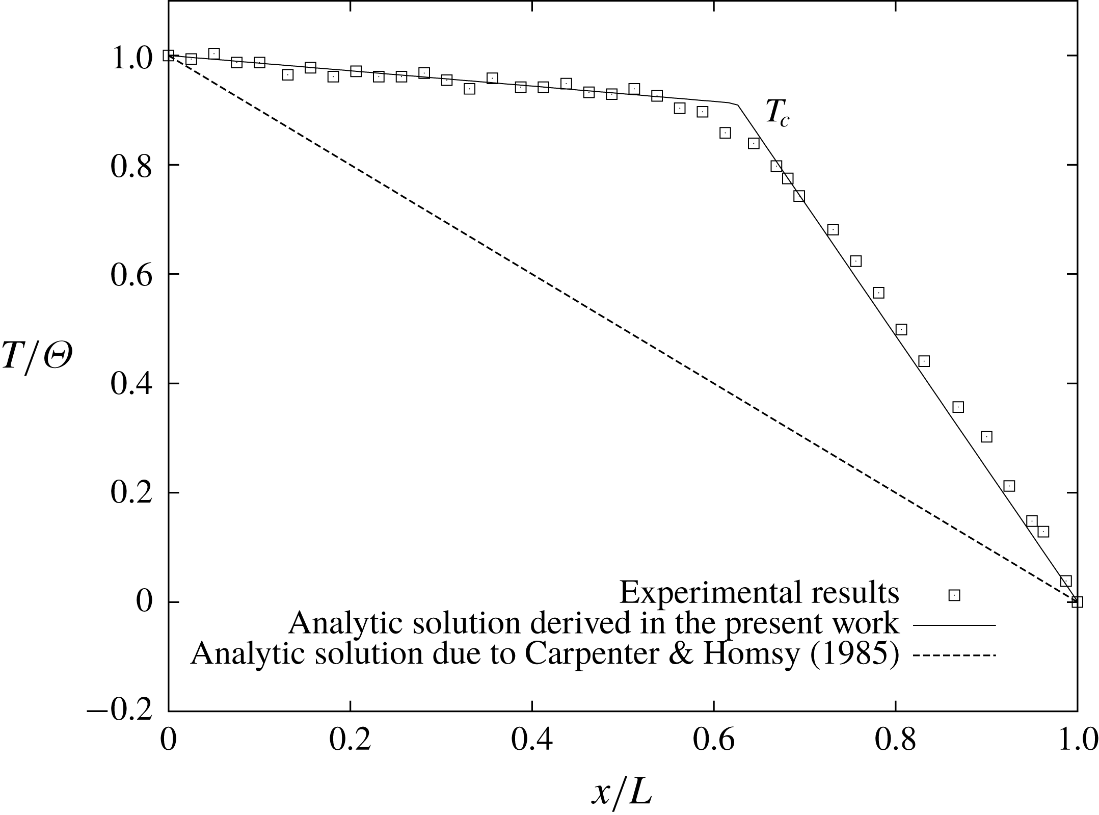
Surface temperature
 $T$
as a function of the horizontal position
 $x/L$
for initial surfactant concentration
 $\unicode[STIX]{x1D6E4}_{0}/\unicode[STIX]{x1D6E4}_{e}=0.1$
and
 $E=0.4$
. Open squares correspond to the experiments with oleic acid. The clearly seen salient point indicates temperature
 $T_{c}$
and coincides with the position of the edge of the stagnant zone
 $x_{c}$
at the surface. Theoretical results are shown with lines. The dashed line represents the analytical result (3.24) obtained by Carpenter & Homsy (Reference Carpenter and Homsy1985) based on the work of Sen & Davis (Reference Sen and Davis1982). The solid line corresponds to the analytical solution obtained in this work (3.25).

However, Shmyrov et al. (Reference Shmyrov, Mizev, Demin, Petukhov and Bratsun2018) have shown that the solution of (3.24) for temperature cannot be realized in practice. The point is that at
 $E<1$
there is a separate stagnant region bounded on one side by the point
 $x=x_{c}$
and on the other by the cold side wall at
 $x=1$
. This means that to the left of the stagnation point (
 $0<x<x_{c}$
) there is a vigorous thermocapillary flow as this area that is free of surfactant and heat is transferred mostly by convection, rather than by heat conductivity. On the other hand, the heat transfer in the stagnation zone
 $x_{c}<x<1$
is carried out almost exclusively by the heat-conductivity mechanism. Our experimental observations support this conclusion (see figures 3 and 9).
Based on these experimental measurements, we have suggested (see Shmyrov et al. (Reference Shmyrov, Mizev, Demin, Petukhov and Bratsun2018)) another analytical solution for (3.18),
 $$\begin{eqnarray}\displaystyle & \displaystyle T_{0}(x)=\boldsymbol{H}(x_{c}-x)\left(1+\frac{T_{c}-1}{x_{c}}x\right)+\boldsymbol{H}(x-x_{c})T_{c}\frac{(1-x)}{(1-x_{c})}, & \displaystyle\end{eqnarray}$$
where
 $T_{c}$
is the dimensionless surface temperature at
 $x=x_{c}$
. Since the relationship between the temperature and the
 $x$
-coordinate is still linear, solution (3.25) also satisfies (3.18) and all of the appropriate boundary conditions (3.19)–(3.22). This means that it is also uniformly valid in the channel as solution (3.24). Moreover, if we put
 $T_{c}=1-x_{c}$
, then the solution (3.25) reduces to the solution (3.24). In fact, equation (3.25) is the simplest equation to take into account the contribution of convection without solving the complete nonlinear convective transfer equation.
In fact, the temperature
 $T_{c}$
has been introduced into the theory as an adjustable parameter to fit the experimental data. On the one hand, the solution (3.24) has been obtained for the motionless fluid and corresponds to the pure heat-conducting regime. Our experiments have shown that the thermocapillary convection significantly distorts an uniform linear temperature distribution. On the other hand, the solution taking into account the contribution of the convection should depend on the Marangoni number and should be obtained already at the leading order. The calculation of the temperature
 $T_{c}$
within the lubrication theory is beyond the scope of this work.
Following the temperature (3.25), the core solution for the streamfunction
 $\unicode[STIX]{x1D713}_{0}$
should also be modified taking into account the surface tangential stress balance (3.23):
 $$\begin{eqnarray}\displaystyle & \displaystyle \unicode[STIX]{x1D713}_{0}(y)=\frac{(1-T_{c})}{6x_{c}}y(y^{2}-3y+2). & \displaystyle\end{eqnarray}$$
Notice that the intensity of the thermocapillary flow depends now on the value of the parameter
 $T_{c}$
. Generally, in order to maintain the flow, it should be
 $T_{c}<1$
. The profile of
 $x$
-component of the velocity is presented in figure 7.
The solution for the surfactant concentration can be obtained by integrating (3.23) with the coordinate
 $x$
taking into account the phase transition,
 $$\begin{eqnarray}\displaystyle \unicode[STIX]{x1D6E4}^{0}(x) & = & \displaystyle -\frac{2}{E}\int _{x_{c}}^{x\boldsymbol{H}(x^{\ast }-x)+x^{\ast }\boldsymbol{H}(x-x^{\ast })}\left.\left(-\frac{\unicode[STIX]{x2202}^{2}\unicode[STIX]{x1D713}_{0}}{\unicode[STIX]{x2202}y^{2}}+\frac{\unicode[STIX]{x2202}T_{0}}{\unicode[STIX]{x2202}x}\right)\right|_{y=0}\text{d}x\nonumber\\ \displaystyle & & \displaystyle -\,\frac{2\boldsymbol{H}(x-x^{\ast })}{kE}\int _{x^{\ast }}^{x}\left.\left(-\frac{\unicode[STIX]{x2202}^{2}\unicode[STIX]{x1D713}_{0}}{\unicode[STIX]{x2202}y^{2}}+\frac{\unicode[STIX]{x2202}T_{0}}{\unicode[STIX]{x2202}x}\right)\right|_{y=0}\text{d}x,\end{eqnarray}$$
where
 $x^{\ast }$
defines a point on the surface when a new phase arises.
3.3 Stagnation point in a one-phase gaseous state
By using the temperature distribution (3.25), solution for the streamfunction (3.26) and calculating the integrals in (3.27), we derive the uniform solution for the concentration of the surfactant being in a one-phase gaseous state
 $$\begin{eqnarray}\displaystyle & \displaystyle \unicode[STIX]{x1D6E4}^{0}(x)=\boldsymbol{H}(x-x_{c})\frac{2T_{c}}{E}\frac{(x-x_{c})}{(1-x_{c})}. & \displaystyle\end{eqnarray}$$
Then we obtain the formula for the stagnation point by integrating the
 $\unicode[STIX]{x1D6E4}_{0}(x)$
given by (3.28) from
 $x=x_{c}$
to
 $x=1$
, using simultaneously the conservation requirement for the surfactant (3.8)
 $$\begin{eqnarray}\displaystyle & \displaystyle x_{c}=1-\frac{1}{T_{c}}E. & \displaystyle\end{eqnarray}$$
It is interesting to compare the solution (3.29) with those obtained by Carpenter & Homsy (Reference Carpenter and Homsy1985)
 $$\begin{eqnarray}\displaystyle & x_{c}=1-\sqrt{E}. & \displaystyle\end{eqnarray}$$
A significant difference between formulas (3.29) and (3.30) is seen. Our result (3.29) suggests stronger compression of the surfactant film due to the greater temperature difference applied to the edges of the stagnant zone. In this area, the thermocapillary effect balances the surface pressure arising in the film. Since the convective flow in the free zone more quickly delivers hot liquid to the edge of the stagnant zone, one observes a significant increase in the temperature difference, which is clearly visible in figure 9. Another difference of (3.29) is the presence of the temperature
 $T_{c}$
. Although the dimensionless value of
 $T_{c}$
is close to unity, this means that a clean surface area appears when the value of the elasticity number
 $E$
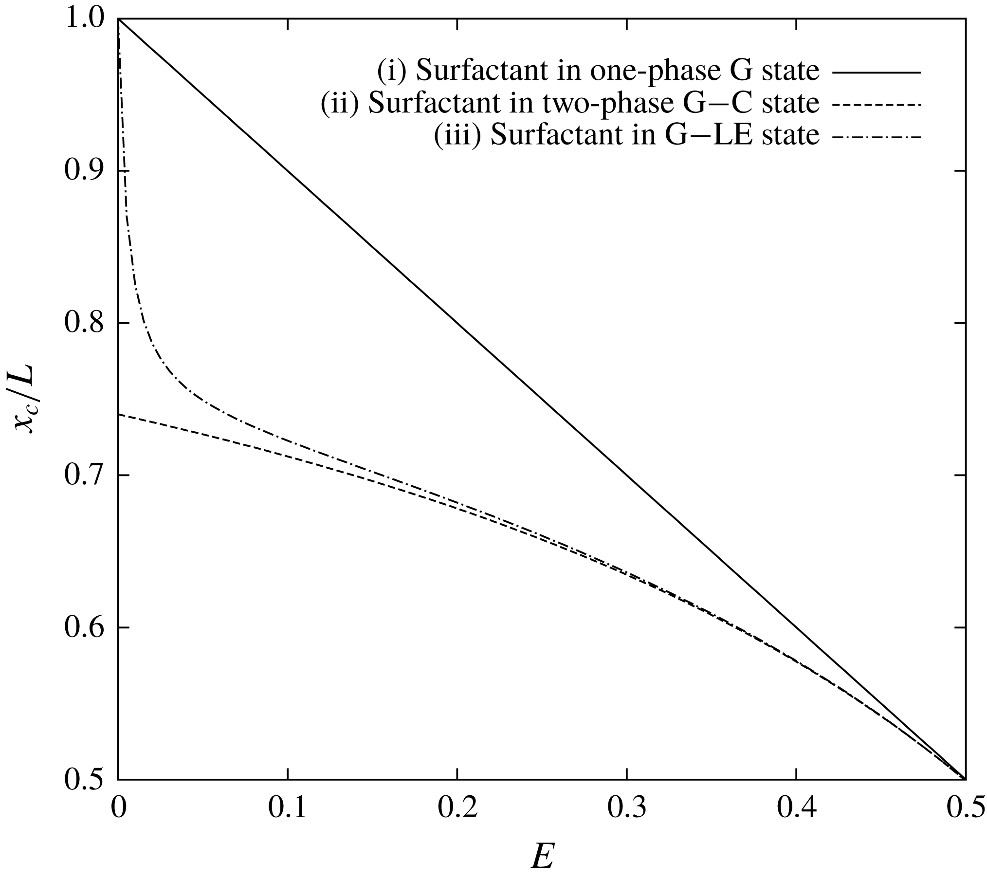
is slightly less than 1. The curve which corresponds to the solution (3.29) is indicated in figure 10 by the solid line (the case (i)).
Dimensionless position of the edge of the stagnant zone
 $x_{c}$
as a function of the elasticity number
 $E$
obtained analytically for three different cases: (i) surfactant in a one-phase gaseous (G) state; (ii) surfactant in a two-phase state composed of gaseous (G) and condensed (C) phases; (iii) surfactant in a two-phase state composed of gaseous (G) and liquid-expanded (LE) phases.
 $E^{\ast }=0.52$
,
 $T_{c}=1$
.

3.4 Stagnation point in a two-phase state composed of gaseous and condensed phases
Clearly, the solution (3.29) is applicable when the value of the elasticity number
 $E$
is close to (but lower than) 1, because the edge of the stagnant zone given by
 $x_{c}$
appears at
 $E=1$
(if
 $T_{c}=1$
). When the elasticity number
 $E$
decreases, the surface pressure in the stagnant zone dramatically increases which triggers a transition of the surfactant from the gaseous state to a more condensed state. The critical value of the elasticity number
 $E^{\ast }$
when the part of the surface film starts to enter into the new phase can be derived from (3.28) in the following form:
 $$\begin{eqnarray}\displaystyle & \displaystyle E^{\ast }=\frac{2T_{c}}{\unicode[STIX]{x1D6E4}^{\ast }}=\frac{2\widetilde{T_{c}}\unicode[STIX]{x1D6E4}_{0}}{\unicode[STIX]{x1D6E9}\widetilde{\unicode[STIX]{x1D6E4}^{\ast }}}, & \displaystyle\end{eqnarray}$$
where
 $\widetilde{\unicode[STIX]{x1D6E4}^{\ast }}$
and
 $\widetilde{T_{c}}$
are the dimensional quantities. It is seen that the critical value of the elasticity number (3.31) is mainly determined by the ratio between the initial concentration of the surfactant
 $\unicode[STIX]{x1D6E4}_{0}$
and the surfactant concentration
 $\unicode[STIX]{x1D6E4}^{\ast }$
at which the phase transition occurs at the surface. It looks quite natural that the value (3.31) is higher at higher temperature difference and at higher initial concentration of the surfactant.
Thus, we can conclude that formula (3.29) can be applied until a phase transition occurs, i.e.
 $E^{\ast }<E<1$
. Let us denote the position of the edge of the second phase in the stagnant zone as
 $x^{\ast }$
. It is evident that
 $x_{c}<x^{\ast }\leqslant 1$
. Now we assume that after the gaseous state the surfactant transfers into to the poorly compressible condensed phase with
 $k\rightarrow \infty$
(it can be figured out as a solid-like state). Then the position of the edge of this solid-like film at the surface is defined by
 $$\begin{eqnarray}\displaystyle & \displaystyle x^{\ast }=x_{c}+\frac{E}{E^{\ast }}(1-x_{c}). & \displaystyle\end{eqnarray}$$
This formula is valid only if
 $E<E^{\ast }$
.
By integrating (3.27), we derive the solution for the surfactant concentration
 $$\begin{eqnarray}\displaystyle & \displaystyle \unicode[STIX]{x1D6E4}^{0}(x)=\frac{2T_{c}}{E(1-x_{c})}(\boldsymbol{H}(x^{\ast }-x)(x-x_{c})+\boldsymbol{H}(x-x^{\ast })(x^{\ast }-x_{c})), & \displaystyle\end{eqnarray}$$
which is applicable to any surface area.
Finally, the analytical solution for the position of the stagnation point
 $x_{c}$
is obtained by integrating the expression for
 $\unicode[STIX]{x1D6E4}^{0}(x)$
(3.33) from
 $x=x_{c}$
to
 $x=1$
and taking into account the conservation requirement (3.8)
 $$\begin{eqnarray}\displaystyle & \displaystyle x_{c}=\boldsymbol{H}(E-E^{\ast })\left(1-\frac{E}{T_{c}}\right)+\boldsymbol{H}(E^{\ast }-E)\left(1-\frac{E^{\ast }}{T_{c}\left(2-{\displaystyle \frac{E}{E^{\ast }}}\right)}\right). & \displaystyle\end{eqnarray}$$
After that we can calculate the location of the phase transition (3.32)
 $$\begin{eqnarray}\displaystyle & \displaystyle x^{\ast }=\boldsymbol{H}(E^{\ast }-E)\left(1-\frac{E^{\ast }-E}{T_{c}\left(2-{\displaystyle \frac{E}{E^{\ast }}}\right)}\right). & \displaystyle\end{eqnarray}$$
The curve which corresponds to the solution (3.34) is indicated in figure 10 (the case (ii)). It is clearly seen that, having arbitrarily strong compression
 $E\rightarrow 0$
of the surfactant film, which can pass into a quasi-solid state, there still exists a region of finite size on the surface for surfactant molecules.
3.5 Stagnation point in a two-phase state composed of gaseous and liquid-expanded phases
Now we derive the solution for the position of the stagnation point
 $x_{c}$
in the case of a two-phase state with a transition from the gaseous phase to the liquid-expanded phase (figure 8). Here we can compare our analytical findings with the experimental results obtained for oleic acid. The estimate for oleic acid gives the value
 $E^{\ast }\approx 0.52$
(
 $T_{c}=1$
,
 $\unicode[STIX]{x1D6E4}_{0}/\unicode[STIX]{x1D6E4}_{e}=0.1$
,
 $\unicode[STIX]{x1D6E4}^{\ast }/\unicode[STIX]{x1D6E4}_{e}=0.38$
). The parameter
 $k$
can be estimated by the known surfactant isotherm shown in figure 2:
 $k\approx 14$
.
By applying the above procedure, the solution for the surfactant concentration is as follows:
 $$\begin{eqnarray}\displaystyle \unicode[STIX]{x1D6E4}^{0}(x) & = & \displaystyle \frac{2T_{c}}{E(1-x_{c})}(\boldsymbol{H}(x^{\ast }-x)(x-x_{c})+\boldsymbol{H}(x-x^{\ast })(x^{\ast }-x_{c}))\nonumber\\ \displaystyle & & \displaystyle +\,\frac{2T_{c}}{kE(1-x_{c})}\boldsymbol{H}(x-x^{\ast })(x-x^{\ast }).\end{eqnarray}$$
The solution for the position of the stagnation point
 $x_{c}$
then is obtained by integrating the expression for
 $\unicode[STIX]{x1D6E4}^{0}(x)$
(3.36) from
 $x=x_{c}$
to
 $x=1$
and taking into account the conservation requirement for the surfactant (3.8)
 $$\begin{eqnarray}\displaystyle x_{c} & = & \displaystyle \boldsymbol{H}(E-E^{\ast })\left(1-\frac{E}{T_{c}}\right)\nonumber\\ \displaystyle & & \displaystyle +\,\boldsymbol{H}(E^{\ast }-E)\left(1-\frac{E^{\ast }}{T_{c}\left({\displaystyle \frac{E}{E^{\ast }}}\left(2-{\displaystyle \frac{E}{E^{\ast }}}\right)+{\displaystyle \frac{1}{k}}\left(1-{\displaystyle \frac{E}{E^{\ast }}}\right)^{2}\right)}\right).\end{eqnarray}$$
After that, using (3.32), we immediately get
 $$\begin{eqnarray}\displaystyle & \displaystyle x^{\ast }=\boldsymbol{H}(E^{\ast }-E)\left(1-\frac{E^{\ast }-E}{T_{c}\left({\displaystyle \frac{E}{E^{\ast }}}\left(2-{\displaystyle \frac{E}{E^{\ast }}}\right)+{\displaystyle \frac{1}{k}}\left(1-{\displaystyle \frac{E}{E^{\ast }}}\right)^{2}\right)}\right). & \displaystyle\end{eqnarray}$$
Dynamics of surfactant phases on the surface depending on the elasticity number
 $E$
obtained analytically for the two-phase state. The change of the stagnant zone edge is indicated by the solid line. The dashed line corresponds to the point of a phase transition from the gaseous (G) state to the liquid-expanded (LE) state. SF stands for the ‘surfactant free’ zone.
 $E^{\ast }=0.52$
,
 $T_{c}=1$
.

The curve which corresponds to the solution (3.37) is indicated in figure 10 (the case (iii)). It is interesting to compare here the curve for the edge of the stagnation zone given by (3.37) with the curve describing the position of the edge of the second phase given by (3.38). The position of the phase transition point
 $x^{\ast }$
is interesting because, unlike the location
 $x_{c}$
, this point cannot be determined experimentally. Thus, the theory here can provide important additional information about the behaviour of the surface phase. Figure 11 shows these curves as a function of the elasticity number. One can see that the more we compress the surfactant film by the fluid flow (
 $E/E^{\ast }\rightarrow 0$
), the closer is the point
 $x^{\ast }$
to the point
 $x_{c}$
. On the assumption of weak compressibility of the liquid-expanded phase, in the limit of small values of the parameter
 $E$
, both curves tend to value
 $x/L=1$
. So, the situation looks like the surfactant film is tightened to a point, and the surface is completely cleaned of surfactant. This limiting case seems to be not realistic since the surfactant is considered to be insoluble. In addition, by compressing the surfactant film by means of the thermocapillary flow, we can use this mechanism only up to a certain limit, established by the achievable temperature difference at the ends of the cavity. Figure 6 clearly shows that the maximal allowable compression, which could be achieved on our experimental set-up, corresponds to
 $E\approx 0.15$
. This value corresponds to the lowest horizontal cross-section of the state diagram shown in figure 11.
Dimensionless position of the stagnant zone
 $x_{c}$
as a function of the elasticity number
 $E$
for the initial dimensionless surfactant concentration
 $\unicode[STIX]{x1D6E4}_{0}/\unicode[STIX]{x1D6E4}_{e}=0.1$
. Open squares correspond to the experiments with oleic acid. Dashed line represents the analytical result by Carpenter & Homsy (Reference Carpenter and Homsy1985) obtained for simple one-phase surfactant layer within a lubrication approximation. The analytical solution (3.37) obtained in the present work is indicated by the solid line.
 $T_{c}=1$
,
 $k=14$
.

Finally, in figure 12, we compare our analytical result (3.37) derived for a two-phase state composed of gaseous and liquid-expanded phases with the experimental data obtained for oleic acid. It is seen that the theoretical curve (solid line) is in perfect agreement with the experimental data both in the range of the gaseous phase
 $0.52<E<1$
and in the range of the liquid-expanded phase
 $E<0.52$
. Figure 12 also shows the curve plotted with the formula (3.30) obtained by Carpenter & Homsy (Reference Carpenter and Homsy1985). As noted above, the deviation of this curve from the experimental data is due to the underestimation of the effect of a sharp increase in the temperature difference applied to the edges of the stagnant zone, due to the intense heat transfer in surfactant-free zone.
4 Numerical study
4.1 Mathematical formulation
In this section, we present a numerical study of the problem to see what happens beyond the limits of applicability of the asymptotic theory presented in the previous section. Thus, we reformulate the problem and change to characteristic scales which are more suitable for the numerical analysis.
Let us consider the incompressible Newtonian liquid filling a rectangular cavity
 $L$
:
 $B$
: 2
 $d$
(figure 13). We further assume that the gap width
 $2d$
is small enough so that the fluid flow may be considered as quasi two-dimensional, i.e. a Hele-Shaw approximation is applicable. The system geometry is represented by a two-dimensional domain with the
 $x$
-axis directed horizontally (
 $0\leqslant x\leqslant L$
) and the
 $y$
-axis anti-directed to gravity (
 $0\leqslant y\leqslant B$
).
Geometrical configuration of the Hele-Shaw cell and coordinate axes.

To formulate the problem for the numerical simulation as close as possible to the experimental conditions, we set the boundary condition for the temperature on the surface in the form of a fixed heat flux, rather than the difference between the known temperatures at the ends of the slot
 $$\begin{eqnarray}\displaystyle & \displaystyle \unicode[STIX]{x1D718}\frac{\unicode[STIX]{x2202}T}{\unicode[STIX]{x2202}y}=A\left(1-\frac{x}{L}\right), & \displaystyle\end{eqnarray}$$
where
 $\unicode[STIX]{x1D718}$
is the coefficient of thermal conductivity,
 $A$
is the heat flux on the left end of the surface
 $x=0$
(figure 12). The heat flux (4.1) varies linearly along the surface, as in the experiments (see figure 1). Since the flux
 $A$
is the only quantity in the problem that can determine the temperature changes, we construct a unit of measurement for the temperature field based on
 $A$
. Thus, we choose the following characteristic scales: length – the semi-gap width
 $d$
, time –
 $d^{2}/\unicode[STIX]{x1D708}$
, velocity –
 $\unicode[STIX]{x1D712}/d$
, temperature –
 $\text{d}A/\unicode[STIX]{x1D718}$
, pressure –
 $\unicode[STIX]{x1D70C}\unicode[STIX]{x1D712}\unicode[STIX]{x1D708}/d^{2}$
, surfactant concentration –
 $\unicode[STIX]{x1D6E4}^{\ast }$
. The mathematical model then consists of the set of dimensionless equations written within the Hele-Shaw and Boussinesq approximations (Gershuni & Zhukhovitskii Reference Gershuni and Zhukhovitskii1976)
 $$\begin{eqnarray}\displaystyle & \displaystyle \frac{\unicode[STIX]{x2202}u}{\unicode[STIX]{x2202}x}+\frac{\unicode[STIX]{x2202}v}{\unicode[STIX]{x2202}y}=0, & \displaystyle\end{eqnarray}$$
 $$\begin{eqnarray}\displaystyle & \displaystyle \frac{\unicode[STIX]{x2202}u}{\unicode[STIX]{x2202}t}+\frac{3}{8\unicode[STIX]{x03C0}\,Pr}\left(u\frac{\unicode[STIX]{x2202}u}{\unicode[STIX]{x2202}x}+v\frac{\unicode[STIX]{x2202}u}{\unicode[STIX]{x2202}y}\right)=-\frac{\unicode[STIX]{x2202}p}{\unicode[STIX]{x2202}x}+\frac{\unicode[STIX]{x2202}^{2}u}{\unicode[STIX]{x2202}x^{2}}+\frac{\unicode[STIX]{x2202}^{2}u}{\unicode[STIX]{x2202}y^{2}}-\frac{\unicode[STIX]{x03C0}^{2}}{4}u, & \displaystyle\end{eqnarray}$$
 $$\begin{eqnarray}\displaystyle & \displaystyle \frac{\unicode[STIX]{x2202}v}{\unicode[STIX]{x2202}t}+\frac{3}{8\unicode[STIX]{x03C0}\,Pr}\left(u\frac{\unicode[STIX]{x2202}v}{\unicode[STIX]{x2202}x}+v\frac{\unicode[STIX]{x2202}v}{\unicode[STIX]{x2202}y}\right)=-\frac{\unicode[STIX]{x2202}p}{\unicode[STIX]{x2202}y}+\frac{\unicode[STIX]{x2202}^{2}v}{\unicode[STIX]{x2202}x^{2}}+\frac{\unicode[STIX]{x2202}^{2}v}{\unicode[STIX]{x2202}y^{2}}-\frac{\unicode[STIX]{x03C0}^{2}}{4}v+Ra\,T, & \displaystyle\end{eqnarray}$$
 $$\begin{eqnarray}\displaystyle & \displaystyle Pr\frac{\unicode[STIX]{x2202}T}{\unicode[STIX]{x2202}t}+\frac{3}{8\unicode[STIX]{x03C0}}\left(u\frac{\unicode[STIX]{x2202}T}{\unicode[STIX]{x2202}x}+v\frac{\unicode[STIX]{x2202}T}{\unicode[STIX]{x2202}y}\right)=\frac{\unicode[STIX]{x2202}^{2}T}{\unicode[STIX]{x2202}x^{2}}+\frac{\unicode[STIX]{x2202}^{2}T}{\unicode[STIX]{x2202}y^{2}}-\frac{\unicode[STIX]{x03C0}^{2}}{4}T. & \displaystyle\end{eqnarray}$$
To average the flow across the Hele-Shaw slot, trigonometric basic functions have been used in (4.2)–(4.5). The boundary conditions for (4.2)–(4.5) are (Birikh et al. Reference Birikh, Briskman, Velarde and Legros2003)
 $$\begin{eqnarray}\displaystyle & \displaystyle x=0:\quad u=0,\quad v=0,\quad \frac{\unicode[STIX]{x2202}T}{\unicode[STIX]{x2202}x}=0,\quad \frac{\unicode[STIX]{x2202}\unicode[STIX]{x1D6E4}}{\unicode[STIX]{x2202}x}=0, & \displaystyle\end{eqnarray}$$
 $$\begin{eqnarray}\displaystyle & \displaystyle x=h:\quad u=0,\quad v=0,\quad \frac{\unicode[STIX]{x2202}T}{\unicode[STIX]{x2202}x}=0,\quad \frac{\unicode[STIX]{x2202}\unicode[STIX]{x1D6E4}}{\unicode[STIX]{x2202}x}=0, & \displaystyle\end{eqnarray}$$
 $$\begin{eqnarray}\displaystyle & \displaystyle y=0:\quad u=0,\quad v=0,\quad \frac{\unicode[STIX]{x2202}T}{\unicode[STIX]{x2202}y}=0, & \displaystyle\end{eqnarray}$$
 $$\begin{eqnarray}\displaystyle & \displaystyle y=b:\quad v=0, & \displaystyle\end{eqnarray}$$
 $$\begin{eqnarray}\displaystyle & \displaystyle \frac{\unicode[STIX]{x2202}u}{\unicode[STIX]{x2202}y}+M_{T}\left(\frac{\unicode[STIX]{x2202}T}{\unicode[STIX]{x2202}x}+Ef(\unicode[STIX]{x1D6E4})\frac{\unicode[STIX]{x2202}\unicode[STIX]{x1D6E4}}{\unicode[STIX]{x2202}x}\right)=0, & \displaystyle\end{eqnarray}$$
 $$\begin{eqnarray}\displaystyle & \displaystyle \frac{\unicode[STIX]{x2202}T}{\unicode[STIX]{x2202}y}=1-\frac{x}{h}, & \displaystyle\end{eqnarray}$$
 $$\begin{eqnarray}\displaystyle & \displaystyle \frac{\unicode[STIX]{x2202}\unicode[STIX]{x1D6E4}}{\unicode[STIX]{x2202}t}+\frac{2}{\unicode[STIX]{x03C0}\,Pr}\frac{\unicode[STIX]{x2202}(u\unicode[STIX]{x1D6E4})}{\unicode[STIX]{x2202}x}=\frac{1}{Sc}\frac{\unicode[STIX]{x2202}^{2}\unicode[STIX]{x1D6E4}}{\unicode[STIX]{x2202}x^{2}}, & \displaystyle\end{eqnarray}$$
where
 $$\begin{eqnarray}\displaystyle & \displaystyle f(\unicode[STIX]{x1D6E4})=1+k\left(1+\text{erf}\left(\frac{\unicode[STIX]{x1D6E4}-1}{\unicode[STIX]{x1D6FF}}\right)\right). & \displaystyle\end{eqnarray}$$
The boundary condition for the tangential stresses (4.10) is written in such a way as to describe the smoothness of the phase transition in the layer instead of the piecewise approximation (3.12) used in the previous section. The parameter
 $\unicode[STIX]{x1D6FF}$
in (4.13) defines the characteristic phase transition width and in simulations it was fixed to the value 0.05. The parameter
 $k$
is equal to 5.
The list of the dimensionless parameters that appeared in (4.2)–(4.12) includes
 $$\begin{eqnarray}\displaystyle Ra=\frac{g\unicode[STIX]{x1D6FD}Ad^{4}}{\unicode[STIX]{x1D708}\unicode[STIX]{x1D712}\unicode[STIX]{x1D718}},\quad Pr=\frac{\unicode[STIX]{x1D708}}{\unicode[STIX]{x1D712}},\quad M_{T}=\frac{\unicode[STIX]{x1D70E}_{T}Ad^{2}}{\unicode[STIX]{x1D702}\unicode[STIX]{x1D712}\unicode[STIX]{x1D718}},\quad E=\frac{\unicode[STIX]{x1D70E}_{\unicode[STIX]{x1D6E4}}\unicode[STIX]{x1D6E4}^{\ast }\unicode[STIX]{x1D718}}{\unicode[STIX]{x1D70E}_{T}dA},\quad Sc=\frac{\unicode[STIX]{x1D708}}{D},\qquad & & \displaystyle\end{eqnarray}$$
the Rayleigh number, the Prandtl number, the thermal Marangoni number, the elasticity number and the surface Schmidt number, respectively. Finally,
 $h$
and
 $b$
stand for the non-dimensional length
 $L/d$
and the height
 $B/d$
of the cavity, respectively.
Equations (4.3) and (4.4) differ from the two-dimensional Navier–Stokes equations by the additional dissipative terms linear in the velocities. These terms in the Hele-Shaw approximation may be interpreted as the average friction force due to the presence of the wide walls of the cavity and they are analogous to the linear velocity term in Darcy’s law valid for fluid flow in porous media. The heat equation (4.5) contains a cooling term that is linear in temperature which relates to the dissipation of heat through the wide walls. This term vanishes if the walls are made of thermo-isolated material and it is maximal if they are highly conductive. By taking into account that the wide walls of the Hele-Shaw cell were typically made of glass, the heat conductivity of which is close to that of the water filling the cavity, one can conclude that heat dissipation during such experiments might be quite intensive.
In order to perform two-dimensional simulations of nonlinear regimes, we apply the vorticity–streamfunction formulation of the governing equations and boundary conditions (4.2)–(4.12), where the streamfunction
 $\unicode[STIX]{x1D6F9}$
is defined as
 $$\begin{eqnarray}\displaystyle & \displaystyle u=\frac{\unicode[STIX]{x2202}\unicode[STIX]{x1D6F9}}{\unicode[STIX]{x2202}y},\quad v=-\frac{\unicode[STIX]{x2202}\unicode[STIX]{x1D6F9}}{\unicode[STIX]{x2202}x}, & \displaystyle\end{eqnarray}$$
and the vorticity
 $\unicode[STIX]{x1D6F7}$
can be calculated using the streamfunction
 $$\begin{eqnarray}\displaystyle & \displaystyle \unicode[STIX]{x1D6F7}=\frac{\unicode[STIX]{x2202}^{2}\unicode[STIX]{x1D6F9}}{\unicode[STIX]{x2202}x^{2}}+\frac{\unicode[STIX]{x2202}^{2}\unicode[STIX]{x1D6F9}}{\unicode[STIX]{x2202}y^{2}}, & \displaystyle\end{eqnarray}$$
 $$\begin{eqnarray}\displaystyle & \displaystyle \frac{\unicode[STIX]{x2202}\unicode[STIX]{x1D6F7}}{\unicode[STIX]{x2202}t}+\frac{3}{8\unicode[STIX]{x03C0}\,Pr}\left(\frac{\unicode[STIX]{x2202}\unicode[STIX]{x1D6F9}}{\unicode[STIX]{x2202}y}\frac{\unicode[STIX]{x2202}\unicode[STIX]{x1D6F7}}{\unicode[STIX]{x2202}x}-\frac{\unicode[STIX]{x2202}\unicode[STIX]{x1D6F7}}{\unicode[STIX]{x2202}y}\frac{\unicode[STIX]{x2202}\unicode[STIX]{x1D6F9}}{\unicode[STIX]{x2202}x}\right)=\frac{\unicode[STIX]{x2202}^{2}\unicode[STIX]{x1D6F7}}{\unicode[STIX]{x2202}x^{2}}+\frac{\unicode[STIX]{x2202}^{2}\unicode[STIX]{x1D6F7}}{\unicode[STIX]{x2202}y^{2}}-\frac{\unicode[STIX]{x03C0}^{2}}{4}\unicode[STIX]{x1D6F7}-Ra\frac{\unicode[STIX]{x2202}T}{\unicode[STIX]{x2202}x}, & \displaystyle\end{eqnarray}$$
 $$\begin{eqnarray}\displaystyle & \displaystyle Pr\frac{\unicode[STIX]{x2202}T}{\unicode[STIX]{x2202}t}+\frac{3}{8\unicode[STIX]{x03C0}}\left(\frac{\unicode[STIX]{x2202}\unicode[STIX]{x1D6F9}}{\unicode[STIX]{x2202}y}\frac{\unicode[STIX]{x2202}T}{\unicode[STIX]{x2202}x}+\frac{\unicode[STIX]{x2202}\unicode[STIX]{x1D6F9}}{\unicode[STIX]{x2202}x}\frac{\unicode[STIX]{x2202}T}{\unicode[STIX]{x2202}y}\right)=\frac{\unicode[STIX]{x2202}^{2}T}{\unicode[STIX]{x2202}x^{2}}+\frac{\unicode[STIX]{x2202}^{2}T}{\unicode[STIX]{x2202}y^{2}}-\frac{\unicode[STIX]{x03C0}^{2}}{4}T. & \displaystyle\end{eqnarray}$$
 $$\begin{eqnarray}\displaystyle & \displaystyle x=0:\quad \unicode[STIX]{x1D6F9}=0,\quad \frac{\unicode[STIX]{x2202}\unicode[STIX]{x1D6F9}}{\unicode[STIX]{x2202}x}=0,\quad \frac{\unicode[STIX]{x2202}T}{\unicode[STIX]{x2202}x}=0,\quad \frac{\unicode[STIX]{x2202}\unicode[STIX]{x1D6E4}}{\unicode[STIX]{x2202}x}=0, & \displaystyle\end{eqnarray}$$
 $$\begin{eqnarray}\displaystyle & \displaystyle x=h:\quad \unicode[STIX]{x1D6F9}=0,\quad \frac{\unicode[STIX]{x2202}\unicode[STIX]{x1D6F9}}{\unicode[STIX]{x2202}x}=0,\quad \frac{\unicode[STIX]{x2202}T}{\unicode[STIX]{x2202}x}=0,\quad \frac{\unicode[STIX]{x2202}\unicode[STIX]{x1D6E4}}{\unicode[STIX]{x2202}x}=0, & \displaystyle\end{eqnarray}$$
 $$\begin{eqnarray}\displaystyle & \displaystyle y=0:\quad \unicode[STIX]{x1D6F9}=0,\quad \frac{\unicode[STIX]{x2202}\unicode[STIX]{x1D6F9}}{\unicode[STIX]{x2202}y}=0,\quad \frac{\unicode[STIX]{x2202}T}{\unicode[STIX]{x2202}y}=0, & \displaystyle\end{eqnarray}$$
 $$\begin{eqnarray}\displaystyle & \displaystyle y=b:\quad \unicode[STIX]{x1D6F9}=0,\quad \frac{\unicode[STIX]{x2202}T}{\unicode[STIX]{x2202}y}=1-\frac{x}{h}, & \displaystyle\end{eqnarray}$$
 $$\begin{eqnarray}\displaystyle & \displaystyle \frac{\unicode[STIX]{x2202}\unicode[STIX]{x1D6E4}}{\unicode[STIX]{x2202}t}+\frac{2}{\unicode[STIX]{x03C0}\,Pr}\frac{\unicode[STIX]{x2202}}{\unicode[STIX]{x2202}x}\left(\unicode[STIX]{x1D6E4}\frac{\unicode[STIX]{x2202}\unicode[STIX]{x1D6F9}}{\unicode[STIX]{x2202}y}\right)=\frac{1}{Sc}\frac{\unicode[STIX]{x2202}^{2}\unicode[STIX]{x1D6E4}}{\unicode[STIX]{x2202}x^{2}}, & \displaystyle\end{eqnarray}$$
 $$\begin{eqnarray}\displaystyle & \displaystyle \unicode[STIX]{x1D6F7}+M_{T}\left(\frac{\unicode[STIX]{x2202}T}{\unicode[STIX]{x2202}x}+E\frac{\unicode[STIX]{x2202}\unicode[STIX]{x1D6E4}}{\unicode[STIX]{x2202}x}+kE\left(1+\text{erf}\left(\frac{\unicode[STIX]{x1D6E4}-1}{\unicode[STIX]{x1D6FF}}\right)\right)\frac{\unicode[STIX]{x2202}\unicode[STIX]{x1D6E4}}{\unicode[STIX]{x2202}x}\right)=0. & \displaystyle\end{eqnarray}$$
4.2 Solution technique
The problem (4.16)–(4.24) has been solved numerically by the finite difference method using a two-field formulation technique. The computational code was written using programming language Fortran-90.
In this study, we consider a Hele-Shaw cell with aspect ratio close to the experimental cuvette:
 $h=12$
,
 $b=5$
. Equations and boundary conditions are approximated on a uniform mesh using a second-order approximation for the spatial coordinates. The nonlinear equations are solved using an explicit scheme on a rectangular uniform mesh. The one-sided and central differences were used to approximate the time and coordinate derivatives, respectively. The typical working mesh contains
 $41\times 27$
nodes. For this number of nodes, we obtained fast and well-converged numerical results. In order to ensure the stability of the numerical scheme, the varying time step is calculated at each iteration by the formula
 $$\begin{eqnarray}\displaystyle & \displaystyle \triangle t=\frac{\triangle x^{2}}{2(2+\max (|\unicode[STIX]{x1D6F9}|,|\unicode[STIX]{x1D6F7}|))}. & \displaystyle\end{eqnarray}$$
The Poisson equations are solved by the iterative Liebman successive over-relaxation method at each time step: the accuracy of the solution is fixed to
 $10^{-4}$
. A noisy streamfunction field
 $\unicode[STIX]{x1D6F9}$
with amplitude less than
 $10^{-3}$
is used in the initial condition. The initial distribution of
 $\unicode[STIX]{x1D6E4}$
is always uniform. The main control parameter of the problem is the thermal Marangoni number
 $M_{T}$
, since this parameter, determined through the heat flux, could easily be changed during the experiments. In all simulation runs, the following parameters were fixed:
 $Ra=600$
,
 $Pr=7$
,
 $Sc=1000$
.
The numerical scheme has been validated by comparing to benchmark numerical solutions. In the case of the square cavity with solid boundaries heated from below considered by De Vahl Davis (Reference De Vahl Davis1983), the average deviation of the streamfunction in the centre was approximately 0.39 % (table 1). The numerical simulation of another problem dealing with the fluid flow in a Hele-Shaw cell elongated along the vertical axis and heated from below (Guenther & Mueller Reference Guenther and Mueller1987) has shown that the average deviation of the Nusselt number was less than 3.42 % (table 2). We have also checked our numerical code by examining the benchmark problem of thermocapillary convection (table 3). A detailed comparison with results of other authors is given in these tables.
Benchmark comparison of numerical codes: streamfunction in the centre of the square cavity heated from below for different values of Rayleigh number.

Benchmark comparison of numerical codes: values of the averaged Nusselt number obtained for different grid resolutions in the Hele-Shaw cell heated from below.
 $Ra=4.2\times 10^{6}$
.

Benchmark comparison of numerical codes: thermocapillary convection in a square cavity differently heated from the side walls.
 $Pr=1$
,
 $Re=10$
.
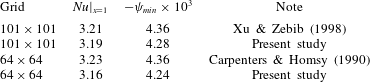
We have also performed a study of the convergence of the numerical results with the gradual refinement of the grid. A typical example of such a study is presented in figure 14. Since most of our calculations have been performed in the range of elasticity number less than 1, the convergence example is presented for the value
 $E=0.6$
when the free surface is slightly open under the action of a thermocapillary flow. One can see that the main grid network
 $41\times 27$
used in this work gives a result within 5 % of the relative error of the value to which the streamfunction converges when the grid is improved. In fact, we have found that this relatively coarse mesh is adequate to insure almost grid-independent results for the flow structure in the bulk of the fluid and the local and overall heat transfer rates, as well as the surfactant concentration and surface velocity distributions. It is important to note that the presence of the surfactant significantly reduces the severe grid packing requirements, which are generally necessary to model pure thermocapillary-induced flows since the boundary conditions transform a significant part of the free surface into a frozen quasi-solid film (Keller & Bergman Reference Keller and Bergman1990).
Convergence of the maximum value of the streamfunction under mesh refinement.
 $E=0.6$
,
 $M_{T}=1600$
.

4.3 Numerical results
Let us first discuss two limiting cases. The first case
 $E=0$
is illustrated in figure 15(a), where the streamfunction isolines are shown. If in (4.16)–(4.24) the elasticity number is set to zero, then these equations are reduced to the problem with a surfactant-free surface and the thermocapillary mechanism of the fluid entrainment induced by heating the surface from above. This problem cannot be reduced completely to the problem considered by Sen & Davis (Reference Sen and Davis1982), since in that work the temperature gradient was applied not only on the surface, but also in its volume. However, in both cases, the main motor of convective motion consists in the thermocapillary effect, which causes the surface to move against the temperature gradient. It should be borne in mind also that (4.16)–(4.24) take into account the effect of gravity. Due to the heat transfer, a non-uniform heating of the surface spreads deep into the fluid layer, where the thermogravitational mechanism begins to work. It is worth noting that the contribution of the thermal convection to the general motion of a fluid in the Hele-Shaw cell has the same sign as the thermocapillary motion: both effects stimulate the circulation of fluid in a clockwise direction (figure 15
a). It is obvious that the thermocapillary effect is stronger than the thermogravitational one, since the maximum of the streamfunction shifts to the surface. The same effect can be seen in the experimental photograph (figure 3
a).
The isolines of streamfunction for the case of the surface not contaminated by any surfactant
 $E=0$
,
 $M_{T}=100$
(a) and the case of the surface fully coated with the surfactant film
 $E=1.1$
,
 $M_{T}=900$
(b).

The streamfunction in the other limiting case, when the entire surface is covered by the surfactant film, is shown in figure 15(b). This effect occurs at any value of the elasticity number greater than 1. As example, figure 15(b) presents the situation for
 $E=1.1$
(
 $M_{T}=900$
). One can notice that in this case the maximum of the streamfunction departs from the interface and shifts deep into the layer. Since the surface is tightly sealed with surfactant, the thermocapillary mechanism of the motion generation can no longer work. The entire surface turns into a stagnant zone, where the fluid practically does not move. At the same time, the non-uniform heating of the layer through the surface continues to work generating thermogravitational convection of the same circulation direction. The intensity of the fluid motion in the cell decreases by approximately one order of magnitude compared with the case
 $E=0$
. In this case, the vortex becomes much more symmetric (figure 15
b). These results obtained numerically are in good qualitative agreement with the experimental observations presented in figure 3(b).
The isolines of streamfunction (a,c,e) and temperature (b,d,f). The rows from top to bottom correspond to
 $E=0.8$
, 0.6, 0.2.

Let us now consider the range of elasticity number values
 $0<E<1$
, at which the surface is only partially covered by the film of surfactant. Figure 16 represents the isolines of the streamfunction and the temperature for three different values of the elasticity parameter from this range. In each of these cases, the whole surface can be divided into two parts with different physical properties. The first zone located on the left in figure 16 is free of surfactant and is characterized by the vigorous fluid movement along the surface. This part of the interface is clearly visible, since the streamlines are concentrated near the surface manifesting a large value of the gradient of the horizontal velocity. The rest of the surface is covered with the surfactant film, and the fluid flow here is significantly hampered. Previously, we have shown (Shmyrov et al.
Reference Shmyrov, Mizev, Demin, Petukhov and Bratsun2018) that the surface velocity in this area, although significantly reduced, is not equal to zero. Slight leakage of fluid through the surfactant film is retained. The main impulse of fluid movement here is shifted deep into the layer. The two characteristic areas on the surface are separated by a narrow transition zone, which was defined above as a stagnation point
 $x_{c}$
. Depending on the flow-induced compression, the stagnation point moves on the surface (compare figure 16
a,b and figure 16
e,f). The decrease of
 $E$
results in the drift of the
 $x_{c}$
in the direction of the colder part of the surface. The same effect can be clearly seen in figure 17, where the surface velocity and temperature are presented as a function of the horizontal coordinate
 $x$
. One can notice that the velocity first rapidly grows, reaching its maximum value approximately in the centre of the surfactant-free area, and then also rapidly decreases when approaching the point
 $x_{c}$
(figure 17
a). To the right of the stagnation point, the velocity
 $u$
is not zero, but due to the figure scaling it is not visible.
The profiles of surface velocity
 $u$
(a) and surface temperature
 $T$
(b) for fixed initial concentration
 $\unicode[STIX]{x1D6E4}=0.1$
. 1 –
 $E=0.2$
; 2 –
 $E=0.4$
; 3 –
 $E=0.6$
; 4 –
 $E=0.8$
.

At first glance, the sequence of temperatures at the left end of the surface looks illogical: the smallest temperature difference corresponds to the maximal width of the surfactant-free surface region (figure 17
b, curve 1). This can be explained by the chosen unit of measurement of temperature, which is based on heat flux
 $A$
. If one presents the temperature in a dimensional form, then this apparent paradox is resolved. Generally, the temperature curves obtained numerically (figure 17
b) look exactly the same as predicted in the framework of the asymptotic theory and measured in experiments (compare with figure 3 and figure 9). This also confirms that our decision to choose the piecewise linear solution for temperature (3.25) was reasonable. The convective transport on the surface is so significant that the temperature cannot remain perfectly linear throughout the entire surface, as was suggested in earlier works. So, the stagnation point is clearly visible in figure 17(b) on the temperature curves, having the characteristic kink. These numerical results are in good qualitative agreement with the experimental observations and analytical research performed in within lubrication-type theory presented above.
Surfactant concentration distribution along the surface for the fixed initial concentration
 $\unicode[STIX]{x1D6E4}_{0}=0.1$
and four different elasticity numbers: 1 – 0.2; 2 – 0.4; 3 – 0.6; 4 – 0.8 (a). Surfactant concentration distribution along the surface for the fixed elasticity number
 $E=0.4$
and three different initial values of
 $\unicode[STIX]{x1D6E4}_{0}$
: 1 – 0.1; 2 – 0.2; 3 – 0.3 (b).

Now we discuss the phase transitions that occur in the surfactant film itself. Figure 18 shows the surfactant concentration as a function of
 $x$
. It clearly illustrates how the phase transition occurs when the elasticity number is varied at the fixed value of the initial surfactant concentration (figure 18
a) or vice versa – when the initial surfactant concentration is varied at a fixed value of the elasticity parameter (figure 18
b). From the point of view of experimental implementation, the first scenario looks more realistic, since it is much easier during the experiment to change the heat flux through the surface than the surfactant concentration. One can see that the surface concentration increases sharply with
 $x$
to the right of the stagnation point. Different inclination angles of the curve can be observed for different values of
 $E$
. Analysing the figure 18, one can notice that the distribution of the surfactant over the surface does not always obey a linear law. This implies that point
 $x_{c}$
is a special point of the system and the situation near it should be investigated separately. Near the point of stagnation, nonlinear deviations become significant: see, for example, curve 2 in figure 18(a) corresponding to
 $\unicode[STIX]{x1D6E4}_{0}/\unicode[STIX]{x1D6E4}^{\ast }=0.1$
and
 $E=0.4$
. The value of the initial concentration
 $\unicode[STIX]{x1D6E4}_{0}/\unicode[STIX]{x1D6E4}^{\ast }=0.1$
means that the number of surfactant molecules is 10 times lower than is necessary for the phase transition. With these values of the parameters, the phase transition to the liquid-expanded phase does not yet occur, since the compression of the film is not yet sufficient. But the compression at
 $E=0.2$
is already enough, and a part of surfactant goes into a new phase state (figure 18
a, curve 1). A phase transition point
 $x^{\ast }$
appears on the surface. Figure 18(b) underlines that the transition to the new phase occurs much easier if the initial concentration of surfactant is higher. If at
 $\unicode[STIX]{x1D6E4}_{0}/\unicode[STIX]{x1D6E4}^{\ast }=0.1$
the entire surfactant film is in a gas phase (figure 18
b, curve 1), then already at
 $\unicode[STIX]{x1D6E4}_{0}/\unicode[STIX]{x1D6E4}^{\ast }=0.3$
almost half of the surface is occupied by the film being in a liquid-expanded state (figure 18
b, curve 3).
Comparison of numerical (solid lines) and experimental (points) results: (a) dependence of the dimensionless coordinate of the stagnant point on the pressure
 $\unicode[STIX]{x03C0}$
applied to the surface due to thermocapillary mechanism; (b) dimensionless position of the edge of the stagnation zone
 $x_{c}$
as a function of the elasticity number
 $E$
for three different values of the initial surfactant concentration
 $\unicode[STIX]{x1D6E4}_{0}/\unicode[STIX]{x1D6E4}_{e}$
: 1 – 0.1; 2 – 0.18; 3 – 0.26.

Now we turn from qualitative to quantitative comparison of the results obtained numerically with the results of the experiments. The positions of the stagnation point
 $x_{c}$
as a function of the surface tension increment
 $\unicode[STIX]{x0394}\unicode[STIX]{x1D70E}_{T}$
due to thermocapillary mechanism and of the elasticity number
 $E$
are presented in figure 19(a) and figure 19(b), respectively. For correct comparison the calculations were done for values of the surfactant surface concentration
 $\unicode[STIX]{x1D6E4}_{0}/\unicode[STIX]{x1D6E4}^{\ast }$
0.26, 0.47 and 0.68, which correspond to the values
 $\unicode[STIX]{x1D6E4}_{0}/\unicode[STIX]{x1D6E4}_{e}$
0.1, 0.18 and 0.26 used in experiments. As in the experiment, under small initial values of
 $\unicode[STIX]{x1D6E4}_{0}/\unicode[STIX]{x1D6E4}_{e}=0.1$
(figure 19
b, curve 1), there exists an almost linear dependence of the stagnation point position on the elasticity number in the interval
 $0.5\lesssim E\leqslant 1$
, where the surfactant is still in the gaseous phase state within the stagnant zone. Further compression of the zone owing to reduction of the elasticity number results in deviation from linearity which is caused by the appearance of the part of the layer with a liquid-expanded phase state. With an increase in the initial surface concentration to
 $\unicode[STIX]{x1D6E4}_{0}/\unicode[STIX]{x1D6E4}_{e}=0.18$
(figure 19
b, curve 2), the part of the layer with the new phase state appears already at
 $x_{c}\approx 0.1$
, which reduces the region of the linear dependence existence significantly. Finally, at
 $\unicode[STIX]{x1D6E4}_{0}/\unicode[STIX]{x1D6E4}_{e}=0.26$
(figure 19
b, curve 3), the surfactant layer near the cold wall is in a liquid-expanded state already at
 $E=1$
, which makes it impossible for a linear dependence region to exist at a given initial concentration of surfactant. It is seen that the results of the numerical simulation are in good quantitative agreement with the experimental data. The same applies to the dependence of the position of the stagnant point on the surface pressure presented in figure 19(a). The curves obtained numerically describe well the experimental results. It is interesting to note that the curves, obtained in calculations, cross the
 $x$
-axis at the values, corresponding to the critical increment of the surface tension
 $\unicode[STIX]{x0394}\unicode[STIX]{x1D70E}_{T}^{\ast }$
, at which the zone free of surfactant appears near the hot edge of the surface. Comparison of these results with those presented in figure 5(a) demonstrates good agreement.
5 Final discussion and conclusions
The influence of non-uniform temperature distribution or surfactant concentration on the motion of a liquid–liquid or liquid–gas interface has been investigated in many works. However, most of the researchers considered separately thermocapillary and solutocapillary effects, and the studies assumed thermal Marangoni convection prevailed.
On the one hand, there is a widely accepted notion that both phenomena are similar, and it is sufficient to study well only one of these effects. The falsity of this approach seems now obvious. Generally speaking, the surfactant dissolved in a liquid volume is separated from the surface by a potential barrier. Once surfactant molecules have passed through this barrier, they can be adsorbed at the interface, where they form a separate surface phase in the case of a soluble surfactant or simply exist at the interface as a separate phase in the case of an insoluble surfactant. This sharply contrasts the behaviour of heat for which there is no potential barrier preventing its access to the interface. The characteristic times of heat and mass diffusion differ by two orders of magnitude, which predetermines different kinetic properties of these fields. Thus, these are essentially different physical phenomena.
On the other hand, an experiment involving generation, maintenance and measurement of concentration fields is more difficult to organize than that for thermal fields. Experts know well how hard it is to achieve, in the solutal case, purity and repeatability of experiments, to quantify surfactant concentrations and to control the course of an experiment. For this reason, experimental studies have been focused on thermocapillary effects for a long time. However, this objective difficulty encountered in the study of solutal Marangoni effects has been gradually overcome with the advent of modern experimental technologies.
From the foregoing it is clear why only few studies were conducted to evaluate the intercoupling of instabilities of thermocapillary and solutocapillary natures. So, the lack of sufficient and reliable data is of great concern to researchers and is one of the motivations of our investigation.
In this work, we have studied the formulated problem for the case where both thermocapillary and solutocapillary effects simultaneously coexist at the interface, and the resulting surface tension gradients are directed towards each other. For simplicity, we confined ourselves to the case of an insoluble surfactant which was chosen in such a way that it was possible to change the phase state in the monolayer under the action of the compressive force from the side of the thermocapillary flow. Usually, the phase transitions in surfactant monolayers are the subject of study in the special literature on physical chemistry. In such works, the mass transfer of surfactant molecules associated with liquid motion is dismissed from consideration from the very beginning, and attention is mainly focused on the kinetic properties of the impurity. Therefore, the assumption made in this paper is an important complication of the standard problem statement in fluid mechanics.
The main difficulty with designing the experiment, which should maximally approximate a theoretical assumption of the linear temperature distribution at the interface, is that the temperature profile between two vertical walls heated to different temperatures is a long way from a linear distribution. We have solved this technical problem by applying an optocapillary method for heating the surface, which made it possible to get for the first time the linear temperature gradient close the ideal one. This approach allowed us to verify the theoretical results obtained in the pioneering work of Carpenter & Homsy (Reference Carpenter and Homsy1985).
It has been found that the theoretical results are in qualitative agreement with the experimental data. When the elasticity parameter becomes
 $E<1$
, the liquid–gas interface can indeed exist simultaneously in two states. The first state is characterized by the fast moving thermocapillary flow, which convects the whole surface-active impurity away. The rest of the surface contains all the surfactant and remains practically motionless. In the latter case, a certain part of the surface can be defined as a stagnant zone. At the same time, the experimental study has revealed a significant deviation from the theoretically predicted position of the stagnation point, which divides the interface into zones. The experimentally measured position of the stagnation point was nearly twice different from the theoretical one. In addition to the quantitative difference, the experimentally obtained curve differs qualitatively so much that the differences cannot be attributed to experimental uncertainties.
The reason for these differences proved to be the real shape of the surface temperature profile, which under Marangoni convection conditions is a piecewise linear function with a kink coincident with the position of the stagnation point. It has been found that the intense thermocapillary flow largely reduces the temperature difference inside the zone free of surfactant. Within the stagnation zone, convection is so weak that the heat transfer occurs almost solely due to the heat-conducting mechanism. Two thermal fields are stitched at the stagnation point. Thus, the temperature profile as a whole remains linear, but it consists of two independent parts. Like the classical solution of Sen & Davis (Reference Sen and Davis1982), our solution also formally satisfies the system of equations in lubrication approximation, but it also takes into account the heterogeneity of surface properties due to the presence of surfactant and relies on our experimental observations.
An important achievement of the work is the experimental results for the elastic properties of the monolayer, part of which can undergo a phase transition during compression under the action of a thermocapillary flow. One part of the monolayer is in a gaseous state, and another part is in a liquid-expanded or -condensed state. The analytical solution for the monolayer structure obtained in the framework of the asymptotic theory, as well as a direct numerical simulation, demonstrated excellent agreement between theory and experiment. Thus, the results obtained in this work cover a fairly wide class of insoluble surfactants and provide a general picture of the dynamics of the monolayer subjected to a surface pressure of a thermocapillary nature under a temperature difference attainable in experiment.
This paper sheds new light on some of the ideas widely accepted by theorists. Practically all of the, not numerous, theoretical works focused on studying the interaction of thermal and solutal Marangoni mechanisms predict the onset of oscillatory instability no matter whether the surfactant is soluble or insoluble (see e.g. Nepomnyashchy, Simanovskii & Legros Reference Nepomnyashchy, Simanovskii and Legros2006). The mechanism responsible for the occurrence of oscillations is based on the competition between two mechanisms driving convective motion (Chen & Shih-Fan Reference Chen and Shih-Fan1992; Nepomnyashchy et al.
Reference Nepomnyashchy, Simanovskii and Legros2006). The surfactant molecules convected by the thermocapillary flow are accumulated at the cold edge of the interface, where the surface tension gradient can locally change its direction, which results in the appearance of a reverse surface flow directed from the cold wall to the hot one. The shift of the stagnation point towards the hot edge causes the reduction in the surfactant surface concentration gradient near the cold edge and thereby the contribution of the thermocapillary mechanism increases. As a result, the surface flow changes its direction near the cold edge and the above process repeats. This type of oscillatory motion has been predicted for
 $E>0.14$
. Although this explanation looks logical and is supported by numerical calculations, we did not observe in our work similar motion mode for any values of elasticity parameter neither in experimental observations nor in numerical simulations. Careful analysis of the problem has revealed that no consideration has been given in the work of Chen & Shih-Fan (Reference Chen and Shih-Fan1992) to the possible phase transition of the surfactant film to new surface phase. It would seem logical that at low initial surface surfactant concentration this effect can be neglected. However, as our results demonstrate, the strong thermocapillary flow can significantly compress the surfactant film on the surface causing a phase transition to a liquid-expanded state with small even zero concentration gradient near the cold wall already in the first seconds of the surface dynamics. No reverse flow may appear in such a situation, and the oscillations identified in the numerical analysis of the theoretical model without phase transitions are only a mathematical artefact. This conclusion, which is based on the results of our investigation, is important by virtue of a widespread idea among theorists that the convective motion should be of oscillatory character in such systems. From this point of view, the result obtained here impels one to critically revise the results of the previous studies and to develop new theoretical models with greater care.
Acknowledgements
D.B. gratefully acknowledges financial support provided by the Ministry of Science and High Education of Russia (grant no. 3.6990.2017/8.9). A.S. and A.M. gratefully acknowledge financial support provided by the Ministry of Science and High Education of Russia (theme no. AAAA-A18-118020590106-3).