1. Introduction
Physical processes that control the degeneration of basin-scale internal gravity waves (IGW) in stratified lakes affected by earth’s rotation have been subject of considerable interest for several decades, owing to their impact on transport and water quality (Wüest & Lorke Reference Wüest and Lorke2003; Boehrer & Schultze Reference Boehrer and Schultze2008). In these aquatic systems, the fundamental IGWs are the known Poincaré and Kelvin waves (Lamb Reference Lamb1932; Csanady Reference Csanady1967), where the latter IGW is usually the most energetic mode (Antenucci & Imberger Reference Antenucci and Imberger2001; Stocker & Imberger Reference Stocker and Imberger2003). Field measurements have shown that the passage of internal Kelvin waves (IKWs) is correlated with high-frequency internal waves (Boegman et al. Reference Boegman, Imberger, Ivey and Antenucci2003; Lorke, Peeters & Bäuerle Reference Lorke, Peeters and Bäuerle2006; de la Fuente et al. Reference de la Fuente, Shimizu, Niño and Imberger2010), shear instabilities and local overturns near the wave troughs in the near-shore regions (Preusse, Peeters & Lorke Reference Preusse, Peeters and Lorke2010; Preusse, Freistühler & Peeters Reference Preusse, Freistühler and Peeters2012a ). These processes lead to significant localized turbulence and mixing in the pelagic thermocline (Lorke Reference Lorke2007; Bouffard & Lemmin Reference Bouffard and Lemmin2013). Over the course of the stratified season, dynamical changes in the wave regime can alter the spatial and temporal distribution of turbulent activity induced by Kelvin waves.
Previous numerical and laboratory studies have analysed the IKW evolution in laminar and weakly nonlinear regimes, obtaining that the wave amplitude, stratification and rotation play an important role in the degeneration and damping processes (de la Fuente et al. Reference de la Fuente, Shimizu, Imberger and Niño2008; Shimizu & Imberger Reference Shimizu and Imberger2009; Sakai & Redekopp Reference Sakai and Redekopp2010; Rozas et al. Reference Rozas, de la Fuente, Ulloa, Davies and Niño2014; Ulloa, de la Fuente & Niño Reference Ulloa, de la Fuente and Niño2014). Here we extend the study of the IKWs to nonlinear regimes at which turbulence starts to emerge, using continuous and smooth solutions that allow control the wavefront steepening and the interfacial shear flow through the initial wave amplitude.
In this study we analyse the degeneration of the ‘gravest internal Kelvin wave’ (hereinafter IKW) in a two-layer stratified basin under different dynamic regimes; from a laminar, linear flow to a nonlinear regime characterized by the transition to turbulence. To this end, we have performed three-dimensional direct numerical simulations (DNS) of the governing equations in a cylindrical domain. The governing equations are the standard three-dimensional Boussinesq equations with
 $m$
-order hyper-viscosity/diffusion operators (Winters & D’Asaro Reference Winters and D’Asaro1997; Waite & Bartello Reference Waite and Bartello2004). The use of a hyper-viscosity/diffusion approach enabled us to increase the scale separation between the forcing and dissipation length scales, producing a larger inertial subrange in the model while confining the dissipation length scales as close as possible to the grid spacing (Spyksma, Magcalas & Campbell Reference Spyksma, Magcalas and Campbell2012). The use of a cylindrical domain permits the derivation of the linear modal structure of IKWs for a discontinuous two-layer stratification (Csanady Reference Csanady1967). This solution was then allowed to diffuse vertically via Laplacian diffusion and molecular diffusivities for mass and momentum for a finite time interval producing slightly smoothed versions of linear normal modes in a continuous, nearly two-layer stratification. The length scale
 ${\it\delta}_{i}$
defines the thickness of the sharp pycnocline, which is constrained to be smaller than the thinner upper layer thickness
 $h_{1}$
. The advantage of this approach is twofold. First, continuous representations of the model solutions are required for the initialization of the numerical model. Second, in calculating the modal solutions, the amplitude of the interface displacement can be taken as a significant fraction of the upper layer thickness without introducing density overturns, whereas if the equations are first linearized about a smooth but sharp density interface, modal amplitudes are restricted to values significantly smaller than the interface scale
 ${\it\delta}_{i}$
.
Figure 1 shows a schematic of the conceptual model, where the subscripts 1 and 2 indicate the upper and lower layer, respectively. The horizontal and vertical length scales are the diameter
 $D$
, equal to twice the radius
 $R$
, and the sum of the two layer thicknesses
 $H=h_{1}+h_{2}$
, respectively;
 ${\it\rho}_{\ell }$
denotes the density of the
 $\ell$
th layer. Rotation is characterized by the inertial frequency
 $f$
, which, together with the linear internal celerity,
 $c_{i}=\sqrt{g^{\prime }h_{1}h_{2}/H}$
, define the internal Rossby radius of deformation,
 $R_{i}=c_{i}/f$
, from the boundary to the interior, where
 $g^{\prime }=g{\rm\Delta}{\it\rho}/{\it\rho}_{1}$
is the reduced gravity and
 ${\rm\Delta}{\it\rho}={\it\rho}_{2}-{\it\rho}_{1}$
. The vertical displacement of the density interface is defined as
 ${\it\eta}_{i}$
, whose maximum initial amplitude is hereinafter denoted by
 ${\it\eta}_{0}=\max \{{\it\eta}_{i}(t=0,\boldsymbol{x})\}$
. Note that because of the spatial structure of IKWs,
 ${\it\eta}_{0}$
occurs at the shoreline (Csanady Reference Csanady1967), i.e. near the vertical sidewalls in our experiments. Our experiments consist of initializing the flow with instantaneous snapshots of smoothed IKW modal solutions at various initial amplitudes
 ${\it\eta}_{0}$
and allowing these initial conditions to evolve under the nonlinear, non-hydrostatic equation of motion.
Schematic of the conceptual model. (a) Three-dimensional view of the domain, a two-layer rotating cylindrical basin of radius
 $R$
and total depth
 $H$
. (b) Two-dimensional plane across a diameter of the basin. (c) Vertical density profile at the centre of the basin (the continuous line denotes a smooth two-layer stratification).

The outline of the paper is as follows. In § 2 we introduce the equations of motion, dimensionless parameters and the set of numerical experiments. In § 3 the IKW response is described in terms of dynamic regimes, while in § 4 we analyse the spatiotemporal distribution of the turbulent activity, focusing on those IKWs in the laminar–turbulent transition regime. Finally, we summarize and discuss our results in § 5.
2. Formulation
2.1. Governing equations and boundary conditions
We study the IKW flow via the numerical solution of the Boussinesq equations of motion for a rotating stratified fluid on an
 $f$
-plane with a
 $m$
-order viscosity/diffusion operator, written as
 $$\begin{eqnarray}\frac{\text{D}\boldsymbol{v}}{\text{D}t}+(f\hat{\boldsymbol{k}})\times \boldsymbol{v}+\frac{{\it\rho}}{{\it\rho}_{0}}g\hat{\boldsymbol{k}}=-\frac{1}{{\it\rho}_{0}}\boldsymbol{{\rm\nabla}}p+{\mathcal{D}}_{m}(\boldsymbol{v}),\quad \frac{\text{D}{\it\rho}}{\text{D}t}={\mathcal{D}}_{m}({\it\rho}),\;\boldsymbol{{\rm\nabla}}\boldsymbol{\cdot }\boldsymbol{v}=0\end{eqnarray}$$
where
 $\text{D}/\text{D}t$
is the material derivative,
 $\boldsymbol{v}=(u,v,w)$
is the velocity vector,
 ${\it\rho}_{0}$
and
 ${\it\rho}$
are the ambient reference density and the Boussinesq density difference from
 ${\it\rho}_{0}$
. Further,
 $p$
is the pressure field,
 $\hat{\boldsymbol{k}}$
is the unit vertical vector (positive upward), whilst
 ${\mathcal{D}}_{m}$
represents an
 $m$
-order viscosity/diffusion operator acting on the momentum and the mass transport, defined as follows (Winters & D’Asaro Reference Winters and D’Asaro1997):
 $$\begin{eqnarray}{\mathcal{D}}_{m}(\cdot )\equiv \left\{\begin{array}{@{}ll@{}}{\it\nu}_{m,j}\partial _{j}^{2m}\quad & \text{dissipation},\\ {\it\kappa}_{m,j}\partial _{j}^{2m}\quad & \text{diffusion},\end{array}\right.\quad \text{with }{\it\nu}_{m,j}={\it\kappa}_{m,j}\equiv \frac{1}{T_{{\mathcal{D}}}}\left(\frac{L_{j}}{{\rm\pi}n_{j}}\right)^{2m},\quad j\in \{x,y,z\},\end{eqnarray}$$
where
 ${\it\nu}_{m,j}$
and
 ${\it\kappa}_{m,j}$
are the
 $m$
-order viscosity/diffusivity coefficient, respectively, whose physical dimensions are
 $[L^{2m}/T]$
. The operator
 $\partial _{j}^{2m}$
corresponds to the
 $2m$
-order partial derivative with respect to the spatial coordinate
 $j$
(with
 $j=x,y,z$
).
 $L_{j}$
and
 $n_{j}$
are the computational domain size and the number of equally spaced grid points in the
 $j$
th direction.
 $T_{{\mathcal{D}}}$
is a time scale chosen by trial and error to minimize the range of damped scales while maintaining numerical stability (Winters & D’Asaro Reference Winters and D’Asaro1997). The choice
 $m=1$
results in the standard Navier–Stokes equations, which should be solved down to the Kolmogorov length scale which is barely possible given the available computing power. Alternatively, for example, the viscosity could be chosen by trial and error to be just large enough to damp the downscale energy transfer for a given problem resolved over a fixed number of grid points. However, if the goal is to allow the inertial subrange to be as broad as possible for a given grid resolution, then larger values of viscosity are inefficient and smaller values require finer grids to resolve the dissipative scales and maintain stability. Similar arguments apply for the
 $m$
-order operators. We use
 $m=3$
for this study and note that the use of this type of closure implicitly assumes a downscale energy cascade with the rate of energy transfer controlled by the nearly inviscid processes in the inertial subrange. This rate can then be measured at small scales by directly evaluating the kinetic energy dissipation rate whose mathematical form depends on the value of
 $m$
chosen as shown in appendix A.
We impose no-flux and free-slip boundary conditions on the top, bottom and sidewalls of the cylindrical domain to avoid having to resolve small viscous boundary layers. The initial condition of the IKW is constructed from the linear normal mode solution derived by Csanady (Reference Csanady1967) for a discontinuous two-layer stratification in a cylindrical domain. This solution is written as
 $$\begin{eqnarray}{\it\eta}_{i}(t,r,{\it\theta})/{\it\eta}_{0}=\text{I}_{1}({\it\beta}_{1}\,r)\,\cos ({\it\theta}-{\it\omega}_{1}t-{\it\phi}),\end{eqnarray}$$
where
 ${\it\eta}_{i}(t,r,{\it\theta})$
is the modal structure of the interface displacement and
 ${\it\beta}_{1}=R_{i}^{-1}\sqrt{1-{\it\sigma}_{1}^{2}}$
. The radial shape of the solution is characterized by the first-kind modified Bessel function of the azimuthal gravest mode,
 $\text{I}_{1}$
(Abramowitz & Stegun Reference Abramowitz and Stegun1965), while the temporal and azimuthal components are given by the cosine periodic function. The wave frequency,
 ${\it\omega}_{1}$
, and dimensionless frequency,
 ${\it\sigma}_{1}={\it\omega}_{1}/f$
, of the IKW are obtained by solving the dispersion relation derived from the boundary condition for
 ${\it\eta}_{i}$
at
 $r=R$
(Csanady Reference Csanady1967; Stocker & Imberger Reference Stocker and Imberger2003):
 $$\begin{eqnarray}1-{\it\sigma}_{1}^{2}\text{M}^{2}=0,\quad \text{with }\text{M}^{2}\equiv {\it\beta}_{1}R\frac{\text{I}_{0}({\it\beta}_{1}R)}{\text{I}_{1}({\it\beta}_{1}R)}-1.\end{eqnarray}$$
From the linearized inviscid governing equations and solution (2.3), we obtain the density and velocity field for a discontinuous two-layer stratification (Csanady Reference Csanady1981; Antenucci & Imberger Reference Antenucci and Imberger2001). However, solution (2.3) cannot be directly used to specify the initial condition of an IKW in a smooth two-layer stratified fluid. Moreover, a derivation of continuous eigenfunctions after introducing a small transition scale
 ${\it\delta}_{i}$
into the density profile is also inconvenient because such solutions are both formally and practically restricted to have displacement amplitudes much smaller than
 ${\it\delta}_{i}$
. Here we wish to study the nonlinear transition regime, and waves in this regime have initial amplitudes substantially larger than
 ${\it\delta}_{i}$
.
For a given
 ${\it\delta}_{i}\ll h_{j},~j=1,2$
, the linear, discontinuous solution (2.3) can be specified with an amplitude
 ${\it\eta}_{0}$
significantly larger than
 ${\it\delta}_{i}$
. We prescribe such a solution, expecting that its subsequent evolution will be nonlinear. We then smooth out the discontinuities by allowing the density and momentum to diffuse over a finite time scale such that the interface thickness is of
 $\mathit{O}({\it\delta}_{i})$
. In contrast, solving the linear equations for a continuously varying but sharply transitioning stratification produces overturns in the density field when
 ${\it\eta}_{0}$
approaches or exceeds
 ${\it\delta}_{i}$
(see e.g. Kundu & Cohen (Reference Kundu and Cohen2004), Chapter 13, on normal modes in a continuously stratified layer).
The equations of motion (2.1), with the smoothed version of the initial condition (2.3), are numerically solved using the three-dimensional spectral model flow_solve (Winters & de la Fuente Reference Winters and de la Fuente2012). The model is based on expansions in terms of trigonometric functions of the dependent variables over regular meshes in a cubic domain (
 $L_{x},L_{y},L_{z}$
), inside which a cylindrical domain (
 $R,H$
) is immersed. The variables are expanded in cosine or sine series in each spatial component, depending on the boundary conditions to be satisfied. For example, in the vertical direction, the horizontal velocity components,
 $u$
and
 $v$
, and the density field,
 ${\it\rho}$
, are expanded in cosine series while the vertical velocity component,
 $w$
, is expanded in sine series to satisfy the free-slip wall and no-flux condition on the top and bottom boundaries. The boundary conditions on the curved sidewall are implemented using an immersed boundary approach introduced by Winters & de la Fuente (Reference Winters and de la Fuente2012).
2.2. Dimensionless numbers
The initial dynamics of the IKW are parametrized by four dimensionless parameters:
 $$\begin{eqnarray}{\mathcal{B}}_{i}\equiv \frac{R_{i}}{R},\quad {\mathcal{T}}_{sk}\equiv \frac{{\it\lambda}_{k}}{{\rm\Delta}c_{i}T_{k}},\quad {\mathcal{T}}_{{\it\nu}k}\equiv \frac{{\it\eta}_{0}^{2m}}{{\it\nu}_{m}T_{k}},\quad {\mathcal{J}}\equiv \frac{{\mathcal{N}}^{2}}{{\mathcal{S}}^{2}}.\end{eqnarray}$$
Here
 ${\mathcal{B}}_{i}$
is the Burger number (Antenucci & Imberger Reference Antenucci and Imberger2001) that characterizes the influence of rotation. If
 ${\mathcal{B}}_{i}\geqslant 1$
, rotation is weak, while if
 ${\mathcal{B}}_{i}<1$
, rotational effects are important. In the IKW case, as
 ${\mathcal{B}}_{i}\rightarrow 0$
, the wave energy becomes concentrated near the boundary with the fluid motions parallel to the shoreline. Notice that
 ${\mathcal{B}}_{i}$
corresponds to the positive root of the classic Burger number,
 $S$
, defined by Pedlosky (Reference Pedlosky1987, see § 1.3, equation 1.3.1).
 ${\mathcal{T}}_{sk}$
is the steepening parameter and it is interpreted as the rate at which the spatial differences of the internal wave celerity induced by
 ${\it\eta}_{0}$
lead to wavefronts and nonlinearities,
 $T_{s}\sim {\it\lambda}_{k}/{\rm\Delta}c_{i}$
, over an IKW period
 $T_{k}$
. Therefore,
 ${\mathcal{T}}_{sk}$
quantifies how fast an IKW with amplitude
 ${\it\eta}_{0}$
tends to produce a nonlinear wavefront (Boegman, Ivey & Imberger Reference Boegman, Ivey and Imberger2005; de la Fuente et al.
Reference de la Fuente, Shimizu, Imberger and Niño2008) and thus to concentrate energy at smaller length scales in the near-shore region.
 $T_{{\it\nu}k}\sim {\it\eta}_{0}^{2m}/{\it\nu}_{m}$
is the dissipation time scale for motions of vertical scale
 ${\it\eta}_{o}$
and
 ${\mathcal{T}}_{{\it\nu}k}$
gives the ratio of this time scale to the Kelvin wave period. To quantify the relative importance of viscous to nonlinear effects in the context of this flow, we have defined a dimensionless number that is the ratio of the (hyper-)viscous time scale to the nonlinear steepening time of the primary Kelvin wave:
 $$\begin{eqnarray}\frac{{\mathcal{T}}_{{\it\nu}k}}{{\mathcal{T}}_{sk}}\equiv \frac{{\rm\Delta}c_{i}{\it\eta}_{0}^{2m-1}}{{\it\nu}_{m}}\left(\frac{{\it\eta}_{0}}{{\it\lambda}_{k}}\right).\end{eqnarray}$$
In this sense, this ratio is similar to the standard Reynolds number that relates inertial to viscous forces. The definition of the
 $m$
-order hyper-viscous Reynolds number is (Lamorgese, Caughey & Pope Reference Lamorgese, Caughey and Pope2005; Spyksma et al.
Reference Spyksma, Magcalas and Campbell2012)
 $$\begin{eqnarray}\mathit{Re}_{m}\equiv \frac{{\rm\Delta}c_{i}{\it\eta}_{0}^{2m-1}}{{\it\nu}_{m}},\end{eqnarray}$$
which formally reduces to the classic viscous Reynolds number when
 $m=1$
:
 $$\begin{eqnarray}\mathit{Re}\equiv \frac{{\rm\Delta}c_{i}{\it\eta}_{0}}{{\it\nu}_{m}}.\end{eqnarray}$$
High values of
 $\mathit{Re}_{m}$
imply energetic regimes, dominated by inertial forces, whereas low values of
 $\mathit{Re}_{m}$
imply flow regimes dominated by (hyper-)viscous forces. The parameter
 ${\mathcal{T}}_{{\it\nu}k}/{\mathcal{T}}_{sk}$
can be written in terms of the hyper-viscous Reynolds number as follows:
 $$\begin{eqnarray}\frac{{\mathcal{T}}_{{\it\nu}k}}{{\mathcal{T}}_{sk}}\equiv \mathit{Re}_{m}\left(\frac{{\it\eta}_{0}}{{\it\lambda}_{k}}\right).\end{eqnarray}$$
Note that
 ${\it\eta}_{0}/{\it\lambda}_{k}$
is the aspect ratio of the Kelvin wave and it is a measure of its hydrostaticity. Steeper, non-hydrostatic waves are more nonlinear and enhance the energy transfer to small scales.
 ${\mathcal{J}}$
is the gradient Richardson number, with
 ${\mathcal{N}}$
the buoyancy frequency and
 ${\mathcal{S}}$
the vertical shear in the horizontal velocity (Miles Reference Miles1961). In our problem, both
 ${\mathcal{N}}$
and
 ${\mathcal{S}}$
have maxima at the height of the density interface but the magnitude and spatial distribution of
 ${\mathcal{J}}$
will depend both on
 ${\it\eta}_{0}$
and
 ${\mathcal{B}}_{i}$
. The maximal shear
 ${\mathcal{S}}$
, for example, occurs in the shore region, near the maximum vertical displacement of the interface. For a fixed rotation regime, the initial minimum value of
 ${\mathcal{J}}$
decreases as
 ${\it\eta}_{0}$
is increased.
The dissipation and mixing involved in the IKW evolution are characterized in terms of dimensionless turbulence activity parameters that quantify the dissipation rates of kinetic energy and buoyancy variance given by
 $$\begin{eqnarray}{\mathcal{I}}_{m}\equiv \frac{1}{{\mathcal{N}}^{2}}\left\{\frac{({\it\epsilon}_{m})^{m}}{{\it\nu}_{m}}\right\}^{2/(3m-1)},\quad {\mathcal{K}}_{m}\equiv |{\rm\nabla}^{m}b|^{2}\,\left|\frac{\text{d}^{m}b}{\text{d}z_{\ast }^{m}}\right|^{-2}\end{eqnarray}$$
where
 ${\mathcal{I}}_{m}$
denotes the turbulence intensity parameter expressed in terms of the hyper-viscosity approach of the kinetic energy dissipation rate,
 ${\it\epsilon}_{m}$
, and derived from the ratio of the Ozmidov and Kolmogorov scales (see appendix A). This parameter can be interpreted as the destabilizing effects of turbulent stirring compared to the stabilizing effects produced by the combined action of hyper-viscosity and buoyancy. Finally,
 ${\mathcal{K}}_{m}$
is the ratio of the diapycnal flux and a reference laminar diffusive flux, both in terms of the hyper-diffusion approach and the buoyancy,
 $b$
. This diffusivity parameter measures the increase in diffusive flux due to turbulent stirring and straining relative to the laminar, diffusive flux with the same background buoyancy that is not stirred or strained (see appendix B).
2.3. Set of numerical experiments
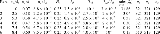
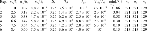
We consider a single rotation regime,
 ${\mathcal{B}}_{i}=0.25$
, and a range of dimensionless amplitudes
 ${\it\eta}_{0}/h_{1}\in [0.07,0.60]$
and aspect ratios
 ${\it\eta}_{0}/{\it\lambda}_{k}\in [8.8\times 10^{-4},7.5\times 10^{-3}]$
that allow
 ${\mathcal{T}}_{sk}\in [3.6,34.6]$
,
 ${\mathcal{T}}_{{\it\nu}k}\in [10^{-1},4\times 10^{4}]$
and initial minimum values of
 ${\mathcal{J}}$
between
 $\min \{{\mathcal{J}}_{0}\}=31.86$
, for
 ${\it\eta}_{0}/h_{1}=0.07$
, and
 $\min \{{\mathcal{J}}_{0}\}=0.13$
, for
 ${\it\eta}_{0}/h_{1}=0.60$
. With these parameters, we have performed six numerical experiments using spatial and temporal scales similar to those used in recent laboratory experiments carried out in a rotating table by Ulloa et al. (Reference Ulloa, de la Fuente and Niño2014). The dimensions of the domain are
 $L_{x}\times L_{y}\times L_{z}=1.95\times 1.95\times 0.2~\text{m}^{3}$
, and in its interior there is a circumscribed cylinder of radius
 $R=0.9~\text{m}$
and depth
 $H=h_{1}+h_{2}=0.07~\text{m}+0.13~\text{m}=0.2~\text{m}$
. The difference of densities is
 ${\rm\Delta}{\it\rho}={\it\rho}_{2}-{\it\rho}_{1}=15~\text{kg}~\text{m}^{-3}$
, the effective thickness of the interfacial transition is
 ${\it\delta}_{i}\approx 0.02~\text{m}$
, and the inertial frequency
 $f=0.361~\text{Hz}$
, with an IKW period of
 $T_{k}=60.45~\text{s}$
and a total simulation time
 $T_{ns}=3T_{k}=182~\text{s}$
. Figure 2 shows that the initial transition layer is resolved by about 12–14 grid points. The horizontal wavelength of the most unstable mode for a smooth, sheared density transition is about
 ${\rm\pi}$
times the interface thickness (see e.g. Kundu & Cohen Reference Kundu and Cohen2004, § 11.7, p. 506). This corresponds to about 10–11 times our horizontal grid spacing and so the most unstable mode is resolved on our spatial grid, though significantly smaller motions are not. Table 2 summarizes the parameters used in the numerical experiments.
Density,
 ${\it\rho}(z)/{\it\rho}$
, and buoyancy frequency,
 ${\mathcal{N}}(z)/\text{max}({\mathcal{N}})$
, profiles in the initial condition of a discontinuous two-layer stratification
 ${\it\delta}_{i}=0$
(grey line) and a smooth two-layer stratification
 ${\it\delta}_{i}>0$
(red line) after a vertical diffusion over a time interval
 $t_{{\it\delta}_{i}}$
. The blue circles denote the equidistant grid points along the transition layer.

Glossary of symbols used in the text.

3. Dynamic regimes
Figure 3 illustrates the time series of a density profile at
 $r/R=0.98$
and
 ${\it\theta}=0$
where
 ${\it\eta}_{i}(t=0,0.98\,R,0)\approx {\it\eta}_{0}$
, and the power spectral density (PSD) of the density interface displacement
 ${\it\eta}_{i}(t,0.98\,xR,0)$
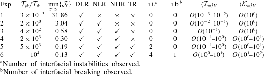
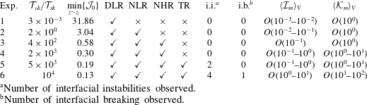
. The IKW response is classified into four distinct regimes: the damped linear (DLR), nonlinear (NLR), nonlinear/non-hydrostatic (NHR) and laminar–turbulent transition regime (TR). The regimes have been defined in terms of their dynamical characteristics
 $({\mathcal{T}}_{sk},{\mathcal{T}}_{{\it\nu}k},{\mathcal{J}})$
and via visual inspection of the density field evolution, similar to the terms in which Horn, Imberger & Ivey (Reference Horn, Imberger and Ivey2001) classified the degeneration of large-scale internal waves in a non-rotating basin. We examine each regime in the following subsections.
(a,c,e,g,i,k) Time series of density field along the vertical profile where the maximum wave amplitude is achieved. (b,d,f,h,k,l) PSD of vertical displacement of density interface
 ${\it\eta}_{i}$
: ▾, Kelvin wave frequency; – ⋅ – ⋅ –, inertial frequency
 $(f/{\it\omega}_{k})$
; – – –, initial buoyancy frequency
 $({\mathcal{N}}_{0}/{\it\omega}_{K})$
; TR, transition regime. (a,b) Exp. 1,
 ${\it\eta}_{0}/h_{1}=0.07$
; (c,d) exp. 2,
 ${\it\eta}_{0}/h_{1}=0.18$
; (e,f) exp. 3,
 ${\it\eta}_{0}/h_{1}=0.38$
; (g,h) exp. 4,
 ${\it\eta}_{0}/h_{1}=0.47$
; (i,j) exp. 5,
 ${\it\eta}_{0}/h_{1}=0.54$
; (k,l) exp. 6,
 ${\it\eta}_{0}/h_{1}=0.60$
.

Summary of the dimensionless parameters of the experimental sets.
3.1. Damped linear regime (DLR)
The DLR is characterized by the evolution of an IKW that retains most of its initial linear features, with negligible nonlinear steepening and strongly controlled by viscosity. This regime describes the results of experiment 1 shown in figure 3(a,b); in this case,
 ${\it\eta}_{0}/h_{1}=0.07~({\it\eta}_{0}/{\it\delta}_{i}\approx 1.0)$
,
 ${\mathcal{T}}_{{\it\nu}k}/{\mathcal{T}}_{sk}\approx 3\times 10^{-3}<1$
and
 $\min \{{\mathcal{J}}_{0}\}\approx 31.86$
, which suggests an extremely viscous flow with a negligible steepening capacity and a strong hydrodynamic stability in the density interface. Therefore a linear and damped IKW dynamics along the
 $3T_{k}$
periods is expected. The PSD in figure 3(b) shows a single strong energy peak at
 ${\it\omega}/{\it\omega}_{k}=1$
, indicating that the initial IKW mode stored the energy of the flow.
3.2. Nonlinear regime (NLR)
The NLR is characterized by weak nonlinear degeneration, without dispersion of the IKW (in the KdV theory sense). This regime starts with the IKW steepening, as a consequence of a wave amplitude large enough to induce significant changes in the wave celerity, leading the wavefront and the formation of a solitary-type wave (Fedorov & Melville Reference Fedorov and Melville1995; de la Fuente et al.
Reference de la Fuente, Shimizu, Imberger and Niño2008). This regime describes the results of experiment 2 shown in figure 3(c,d); in this case
 ${\it\eta}_{0}/h_{1}=0.18$
,
 ${\mathcal{T}}_{{\it\nu}k}/{\mathcal{T}}_{sk}\approx 1.9>1$
and
 $\min \{{\mathcal{J}}_{0}\}\approx 3.04$
, and therefore we expect a weakly nonlinear steepening controlled by viscosity and a stable flow around the density interface. In fact, figure 3(c) shows a slightly steep wavefront after the first wave period and a solitary-type wave structure around
 $t/T_{k}\approx 2.45$
. The PSD in figure 3(d) shows a wider energy cascade due to transfer of energy involved in the weakly nonlinear degeneration, with a main energy peak at
 ${\it\omega}/{\it\omega}_{k}=1$
, and two lower peaks of sub-inertial frequencies attributed to sub-azimuthal Kelvin waves (see the dot-dashed line).
3.3. Nonlinear and non-hydrostatic regime (NHR)
Nonlinear steepening and non-hydrostatic dispersion of the initial IKW (in the KdV theory sense) characterize the NHR. As the wave steepens, its azimuthal length scale decreases until the non-hydrostatic terms can be important enough to balance the nonlinear steepening, avoiding the wave breaking (Helfrich & Melville Reference Helfrich and Melville2006) and leading the degeneration of the IKW into a package of solitary-type waves (Grimshaw Reference Grimshaw1985). This process induces an important energy cascade from the basin scale to smaller scales. The NHR regime is identified in experiments 3–6 (see figures 3
e–l). In these experiments the Reynolds number increases from
 ${\mathcal{T}}_{{\it\nu}}/{\mathcal{T}}_{s}\approx 4\times 10^{2}$
, for
 ${\it\eta}_{0}/h_{1}=0.38$
, to
 ${\mathcal{T}}_{{\it\nu}k}/{\mathcal{T}}_{sk}\approx 10^{4}$
, for
 ${\it\eta}_{0}/h_{1}=0.60$
. Increasing
 ${\mathcal{T}}_{{\it\nu}}/{\mathcal{T}}_{s}$
corresponds to increasing nonlinearity and concentration of energy at smaller scales. Experiments 3 and 4 show hydrodynamic stable flows in the density interface region, with
 $\min \{{\mathcal{J}}_{0}\}\approx 0.58$
and
 $\min \{{\mathcal{J}}_{0}\}\approx 0.30$
, respectively, whereas experiments 5 and 6 show evidence of the emergence of hydrodynamic interfacial instabilities, with
 $\min \{{\mathcal{J}}_{0}\}\approx 0.20$
and
 $\min \{{\mathcal{J}}_{0}\}\approx 0.13$
, respectively.
3.4. Laminar–turbulent transition regime (TR)
The TR is characterized by the growth and occurrence of interfacial instabilities. Depending on how energetic the shear flow is, the instabilities can grow and generate turbulent patches in the density interface region or can be damped. The hydrodynamic stability of the IKW sheared flow can be studied via the gradient Richardson number,
 ${\mathcal{J}}$
, whose critical value
 ${\mathcal{J}}=0.25$
(Miles Reference Miles1961) is neither a necessary nor a sufficient condition to trigger interfacial instabilities in our sheared-type flow, but it is still a very useful criterion that can give us an order of magnitude. In our results only two experiments show the presence of interfacial instabilities, experiments 5 and 6, with
 $\min \{{\mathcal{J}}_{0}\}\approx 0.20$
and
 $\min \{{\mathcal{J}}_{0}\}\approx 0.13$
, respectively. Only they have initial
 ${\mathcal{J}}<0.25$
. Both experiments exhibit the emergence of Kelvin–Helmholtz-type billows on the wavefront of strongly nonlinear IKWs (
 ${\mathcal{T}}_{{\it\nu}k}/{\mathcal{T}}_{sk}\sim 5\times 10^{3}{-}10^{4}$
). However, the results of experiment 5 show fast damping of the interfacial instabilities, while the results of experiment 6 show a complex spatial and temporal dynamic, in which large scales, attributed to the IKW and internal solitary-type waves, coexist and interplay with turbulent small scales, associated with interfacial instabilities/breaking and turbulent patches.
Results of experiment 6: evolution in time
 $t/T_{k}\in [0,3]$
of the vertical velocity
 $w$
at the density interface region
 ${\it\rho}(t,\boldsymbol{x})={\rm\Delta}{\it\rho}/2$
. (a)
 $t/T_{k}=0$
, (b)
 $t/T_{k}=0.128$
, (c)
 $t/T_{k}=0.25$
, (d)
 $t/T_{k}=0.5$
, (e)
 $t/T_{k}=0.75$
, (f)
 $t/T_{k}=1.0$
, (g)
 $t/T_{k}=1.5$
, (h)
 $t/T_{k}=1.75$
, (i)
 $t/T_{k}=2.0$
, (j)
 $t/T_{k}=2.25$
, (k)
 $t/T_{k}=2.75$
, (l)
 $t/T_{k}=3.0$
.

The first three regimes have been analysed in previous numerical (de la Fuente et al. Reference de la Fuente, Shimizu, Imberger and Niño2008; Sakai & Redekopp Reference Sakai and Redekopp2010) and experimental studies (Wake, Ivey & Imberger Reference Wake, Ivey and Imberger2005; Ulloa et al. Reference Ulloa, de la Fuente and Niño2014), whereas the TR on IKWs has been observed only in field data (Lorke Reference Lorke2007; Preusse et al. Reference Preusse, Peeters and Lorke2010) and to date in numerical experiments.
4. Internal Kelvin wave: transition from laminar to turbulent regime
Hereafter we focus on the spatial and temporal evolution of the IKW in the TR (analysing results of experiment 6), aiming to link the dynamic wave response with turbulent activity. Figure 4 shows the evolution of the vertical velocity,
 $w(t,r,{\it\theta},z)$
, at the density interface
 $z_{i}$
to illustrate the strongly nonlinear dynamics of the IKW in experiment 6. Here
 $z_{i}(t)$
is defined as the vertical position of the
 ${\it\rho}(t,\boldsymbol{x})={\rm\Delta}{\it\rho}/2$
iso-scalar surface. Figure 4(a) shows the initial condition of the IKW (
 $t/T_{k}=0$
). The degeneration of the IKW begins with the emergence of instabilities of Kelvin–Helmholtz (KH) type on the wavefront that starts to steepen at
 $t/T_{k}=0.128$
(see figure 4
b); it is in this region where the minimum Richardson number,
 ${\mathcal{J}}\approx 0.13$
, is achieved. Figures 4(c) and 4(d) (
 $t/T_{k}\in [0.25,0.5]$
) show the formation of a turbulent patch induced by the breakdown of the KH-type billows; this patch evidences a slight spread along the azimuthal and radial axes. Figure 4(d) shows the formation of the first solitary-type wave around
 $t/T_{k}\in [0.5,0.625]$
, while figures 4(e) and 4(f) show a solitary wave train confined to the near-shore region around
 $t/T_{k}\in [0.75,1.0]$
. After the first IKW period (see figure 4
f,g) the leading wave starts to interact with the pre-existing turbulent patch. This interaction is accompanied by the regrowth of interfacial instabilities upstream of the wavefront and a subsequent interfacial turbulent wake on the solitary wave train (see figure 4
g). The regrowth of interfacial instabilities generate a new turbulent patch that holds the same azimuthal location while it is vertically advected upward and downward by the solitary wave train (see figure 4
h). During and after the interaction between the large internal waves and the turbulent patch, inertial waves of different scales are radiated to the offshore region (see figure 4
h–k). At
 $t/T_{k}=3$
(see figure 4
l) there is no longer evidence of the initial IKW; the internal waves in the near-shore region have decayed in amplitude, whilst a range of smaller length scales have been excited in the interior. During the first three IKW periods we observe that different nonlinear processes coexist, enhancing the degeneration of the initial long wave and promoting a forward energy cascade.
4.1. Spatiotemporal distribution of turbulence
Figure 5 shows the vertical average of the turbulence intensity parameter,
 $\langle {\mathcal{I}}_{m}\rangle _{H}$
; the dashed line defines the radial position of the internal Rossby radius of deformation,
 $R_{i}$
, from the boundary to the interior. Figure 5(a) shows the initial distribution of
 $\langle {\mathcal{I}}_{m}\rangle _{H}$
induced by the IKW itself. Kinetic energy dissipation is concentrated within
 $R_{i}$
and decays to low values towards the centre of the domain. The nonlinear dynamics of the IKW induces distinct zones of elevated values in the near-shore region, associated with turbulent patches produced by the breakdown of interfacial instabilities (see figure 5
b–d). As the initial IKW degenerates, the turbulence intensity increases at the front of each solitary-type wave along the shore region (see figure 5
d–f) achieving values of
 $\langle {\mathcal{I}}_{m}\rangle _{H}\sim \mathit{O}(10^{2})$
, while most of the offshore region shows a low activity with values of
 $\langle {\mathcal{I}}_{m}\rangle _{H}\sim \mathit{O}(10^{-1})$
. However, after the first period, and particularly after the strong reactivation of the pre-existing turbulent patch, there is a steady increase of
 $\langle {\mathcal{I}}_{m}\rangle _{H}$
to the interior of
 $R_{i}$
, with values in the range
 $\mathit{O}(10^{0})\leqslant \langle {\mathcal{I}}_{m}\rangle _{H}\leqslant \mathit{O}(10^{1})$
(see figure 5
f–h). This process is again observed after the second period (see figure 5
j). After three periods elevated values of
 $\langle {\mathcal{I}}_{m}\rangle _{H}$
are distributed throughout the domain (see figure 5
k,l). Nevertheless, there are clear differences in the intensity between the near-shore and interior regions, where the internal Rossby radius of deformation (dashed line) seems to define a transition length scale of the turbulent activity along the radial component.
Results of experiment 6: spatiotemporal distribution of the turbulence intensity,
 $\langle {\mathcal{I}}_{m}\rangle _{H}$
. (a)
 $t/T_{k}=0$
, (b)
 $t/T_{k}=0.128$
, (c)
 $t/T_{k}=0.25$
, (d)
 $t/T_{k}=0.5$
, (e)
 $t/T_{k}=0.75$
, (f)
 $t/T_{k}=1.0$
, (g)
 $t/T_{k}=1.5$
, (h)
 $t/T_{k}=1.75$
, (i)
 $t/T_{k}=2.0$
, (j)
 $t/T_{k}=2.25$
, (k)
 $t/T_{k}=2.75$
, (l)
 $t/T_{k}=3.0$
.

The azimuthal distribution of the turbulence intensity parameter has features of baroclinic instabilities. This is also observed in figure 6, which shows the relative vertical vorticity,
 ${\bf\omega}\boldsymbol{\cdot }\hat{\boldsymbol{k}}$
, normalized by
 $f$
at
 $z/H=0.8$
(horizontal plane) and the density interface structure
 ${\it\rho}(t,\boldsymbol{x})={\rm\Delta}{\it\rho}/2$
in purple. Initially we observe the formation of one turbulent patch in the shore region around
 $t/T_{k}=0.25$
(see figure 6
c), which grows and spreads along the shore until approximately the first period (see figure 6
d–f). After the first period, the initial turbulent patch is separated into two (see figure 6
d,h,i) that also remain trapped on the shore, and a third vortex structure grows on the shore region during the second period (see figure 6
k,l). It is observed that turbulent patches tend to aggregate in large horizontal motions that scale with
 $R_{i}$
. Figure 6(m) shows a close-up of the vertical vorticity at
 $t/T_{k}=3$
, where three large-scale vortex-type motions are identified in the near-shore region (see dashed ellipses). We can study the existence of baroclinic instability via a simplified model. Pedlosky (Reference Pedlosky1970) considered a quasi-geostrophic two-layer model in an inviscid flow rotating on an
 $f$
-plane, with uniform velocities
 $U_{1}$
and
 $U_{2}$
in each layer
 $(U_{1}\neq U_{2})$
. The flow is unstable to disturbances with horizontal wavelengths,
 ${\it\lambda}$
, larger than
 ${\rm\pi}R_{i}$
(see e.g. Pedlosky Reference Pedlosky1987, Chapter 7, p. 556). Then, considering the azimuthal wavelength of the IKW,
 ${\it\lambda}_{k}=2{\rm\pi}R$
, and the internal Rossby radius here adopted, it is obtained that the flow induced by the IKW admits the growth of baroclinic instabilities because
 ${\rm\pi}R_{i}/{\it\lambda}_{k}={\mathcal{B}}_{i}/2=0.125$
. In addition, the interaction between the vortex-type motions and the vertical shear flow driven by the IGW could be supporting the emergence of baroclinic instabilities (Sakai Reference Sakai1989; Gula, Plougonven & Zeitlin Reference Gula, Plougonven and Zeitlin2009; Flór, Scolan & Gula Reference Flór, Scolan and Gula2011). Note that these large-scale vortex motions are not observed in the interior of the basin.
Results of experiment 6: spatiotemporal distribution of the vertical vorticity,
 $({\bf\omega}/f)\boldsymbol{\cdot }\hat{\boldsymbol{k}}$
, at
 $z/H=0.80$
. (a)
 $t/T_{k}=0$
, (b)
 $t/T_{k}=0.128$
, (c)
 $t/T_{k}=0.25$
, (d)
 $t/T_{k}=0.5$
, (e)
 $t/T_{k}=0.75$
, (f)
 $t/T_{k}=1.0$
, (g)
 $t/T_{k}=1.5$
, (h)
 $t/T_{k}=1.75$
, (i)
 $t/T_{k}=2.0$
, (j)
 $t/T_{k}=2.25$
, (k)
 $t/T_{k}=2.75$
, (l)
 $t/T_{k}=3.0$
, (m)
 $t/T_{k}=3.0$
.

Figure 7 shows the time series of extreme and bulk values of the turbulence intensity parameter, within and outside
 $R_{i}$
. The red vertical lines identify events (
 $e_{i}$
) with high turbulent activity (local maxima) in the time series of experiment 6 (–
 $\bullet$
–), whose horizontal positions can be identified in figure 5(b,d,g,i,j). In figure 7(a) the values of
 $\min \{{\mathcal{I}}_{m}\}$
are comparable for all experiments except experiments 1 and 2 (blue lines), with
 $\min \{{\mathcal{I}}_{m}\}\sim \mathit{O}(10^{3})$
. Values of
 $\max \{{\mathcal{I}}_{m}\}$
, however, increase with increasing nonlinearity, causing the separation of the time series between
 $\mathit{O}(10^{-1})\leqslant \max \{{\mathcal{I}}_{m}\}\leqslant \mathit{O}(10^{2})$
(red lines). In the case of experiment 6, peak turbulence intensity values are
 $\mathit{O}(10^{5})$
times the background laminar value. These results show a significant heterogeneity of
 ${\mathcal{I}}_{m}$
in both time and space. We have divided the domain into two volumes:
 $V_{in}$
and
 $V_{out}$
denote the volumes within and outside
 $R_{i}$
, respectively, and over these volumes bulk quantities of
 ${\mathcal{I}}_{m}$
have been calculated. Within
 $R_{i}$
(see figure 7
b), time series of
 $\langle {\mathcal{I}}_{m}\rangle _{V_{in}}$
show distinct differences between each experiments. The highest values and the most interesting temporal fluctuations are observed in experiment 6 (–
 $\bullet$
–). Outside
 $R_{i}$
(see figure 7
c), time series show that
 $\langle {\mathcal{I}}_{m}\rangle _{V_{out}}$
tends to grow as a function of time, and shows only one peak at
 $e_{2}$
attributed to the formation of the first turbulent patch; figure 5(d) shows that this event (
 $e_{2}$
) affects a small region outside
 $R_{i}$
. Comparing both volumes, early in time, the distinction between the turbulent activity within and outside
 $R_{i}$
is quite important, but by the later times in the experiments,
 ${\mathcal{I}}_{m}$
is only about a factor of 3 higher (see figure 7
b,c for the most energetic case) and the tendency is to reduce the difference between both regions.
Evolution in time (scaled by
 $T_{K}$
) of (a) the maximal and minimal values of the turbulence intensity parameter, (b) the bulk turbulence intensity parameter within
 $R_{i}$
,
 $\langle {\mathcal{I}}_{m}\rangle _{V_{in}}$
, and (c) the bulk turbulence intensity parameter outside
 $R_{i}$
,
 $\langle {\mathcal{I}}_{m}\rangle _{V_{out}}$
. Legend: –
 $\bullet$
–, exp. 6; –
 $+$
–, exp. 5; –▼–, exp. 4; –
 $\times$
–, exp. 3; –▪–, exp. 2; –♦–, exp. 1.

4.2. Turbulence intensity and effective diffusivity
Figures 8(a) and 8(b) show time series of the bulk averages of the turbulence intensity parameter,
 $\langle {\mathcal{I}}_{m}\rangle _{V}$
, and the diffusivity parameter,
 $\langle {\mathcal{K}}_{m}\rangle _{V}$
, respectively.
Evolution in time (scaled by
 $T_{K}$
) of (a) the bulk turbulence intensity parameter,
 $\langle {\mathcal{I}}_{m}\rangle _{V}$
, and (b) the bulk diffusivity parameter,
 $\langle {\mathcal{K}}_{m}\rangle _{V}$
. Panel (c) exhibits
 $\langle {\mathcal{K}}_{m}\rangle _{V,T}$
versus
 $\langle {\mathcal{I}}_{m}\rangle _{V,T}$
. Legend: –
 $\bullet$
–, exp. 6; –
 $+$
–, exp. 5; –▼–, exp. 4; –
 $\times$
–, exp. 3; –▪–, exp. 2; –♦–, exp. 1.

The temporal structure of
 $\langle {\mathcal{I}}_{m}\rangle _{V}$
(see figure 8
a) is forced by the turbulent activity in the near-shore region (see peaks denoted by vertical dashed lines) but with lower magnitudes because of the low turbulent activity on the offshore region. Meanwhile, the time series of
 $\langle {\mathcal{K}}_{m}\rangle _{V}$
can be clustered into three groups (see figure 8
b): a first group with experiments 1–3, a second group with experiments 4–5 and a third group with experiment 6. The first group contains experiments with the lowest and almost constant value of
 $\langle {\mathcal{K}}_{m}\rangle _{V}$
, the second includes experiments with weak fluctuations of
 $\langle {\mathcal{K}}_{m}\rangle _{V}$
, and the third group has the highest values and the strongest fluctuations of
 $\langle {\mathcal{K}}_{m}\rangle _{V}$
. Experiment 6 is unique in that it yields substantially increased values of
 $\langle {\mathcal{K}}_{m}\rangle _{V}$
that are clearly correlated with individual breaking events (–
 $\bullet$
– and vertical dashed line in figure 8
b). The temporal structure of
 $\langle {\mathcal{K}}_{m}\rangle _{V}$
indicates that episodic increases of the bulk diffusivity parameter are not directly correlated with the bulk-averaged turbulence intensity.
Figure 8(c) shows the volumetric and temporal averages,
 $\langle \cdot \rangle _{V,T}$
, of
 ${\mathcal{I}}_{m}$
and
 ${\mathcal{K}}_{m}$
. Red symbols correspond to
 $\langle {\mathcal{K}}_{m}\rangle _{V,T}$
against
 $\langle {\mathcal{I}}_{m}\rangle _{V,T}$
while the clusters of symbols around each red symbol correspond to
 $\langle {\mathcal{K}}_{m}\rangle _{V}(t)$
against
 $\langle {\mathcal{I}}_{m}\rangle _{V}(t)$
(data shown in figure 8
a,b). Further, the standard deviations (s.d.) of the bulk values
 $\langle \cdot \rangle _{V}$
over time are shown (bars in the red symbols). We only see significant temporal variability in experiment 6, shown by –
 $\bullet$
– in figure 8(b) and the cluster of circles in figure 8(c). The large deviations seen in experiment 6 are a consequence of having approximately steady values of turbulence intensity (see figure 8
a) but with very episodic elevated mixing (see figure 8
b), suggesting that an instantaneous and local sampling of dissipation can be very misleading in terms of predicting the instantaneous mixing rate. On the other hand, averaging over all the events we identify a simple relation between
 $\langle {\mathcal{K}}_{m}\rangle _{V,T}$
and
 $\langle {\mathcal{I}}_{m}\rangle _{V,T}$
. For values of
 $\mathit{O}(10^{-2})\leqslant \langle {\mathcal{I}}_{m}\rangle _{V,T}\leqslant \mathit{O}(10^{-1})$
we find that
 $\langle {\mathcal{K}}_{m}\rangle _{V,T}\sim \mathit{O}(10^{0})$
, i.e. that the total diffusivity is not substantially elevated over that expected by laminar diffusion. For
 $\mathit{O}(10^{-1})\leqslant \langle {\mathcal{I}}_{m}\rangle _{V,T}\leqslant \mathit{O}(10^{1})$
, however, the observed diffusivity is greater than that expected in a laminar flow and increases approximately linearly with turbulence intensity. The data fit a power law
 $\langle {\mathcal{K}}_{m}\rangle _{V,T}\sim a\{\langle {\mathcal{I}}_{m}\rangle _{V,T}\}^{b}$
, with parameters
 $a=12.2$
and
 $b=1.1$
. In the next subsection we describe the Kelvin wave evolution in the near-shore region and analyse the vertical distribution of
 ${\mathcal{I}}_{m}$
during the events
 $e_{2}$
and
 $e_{3}$
.
Results of experiment 6: evolution in time
 $t/T_{k}\in [0,3]$
of the stratification,
 ${\mathcal{N}}^{2}/{\mathcal{N}}_{0}^{2}$
, in the area
 ${\it\theta}\in [0,2{\rm\pi}]$
,
 $z/H\in [0,1]$
at
 $r/R=0.98$
. (a)
 $t/T_{k}=0$
, (b)
 $t/T_{k}=0.128$
, (c)
 $t/T_{k}=0.25$
, (d)
 $t/T_{k}=0.5$
, (e)
 $t/T_{k}=0.75$
, (f)
 $t/T_{k}=1.0$
, (g)
 $t/T_{k}=1.128$
, (h)
 $t/T_{k}=1.5$
, (i)
 $t/T_{k}=2.0$
, (j)
 $t/T_{k}=2.25$
, (k)
 $t/T_{k}=2.75$
, (l)
 $t/T_{k}=3.0$
.

4.3. Flow evolution in the near-shore region
Figure 9 shows a summary of the vertical stratification in experiment 6,
 ${\mathcal{N}}^{2}/{\mathcal{N}}_{0}^{2}$
(where
 ${\mathcal{N}}_{0}^{2}\equiv \max \{{\mathcal{N}}^{2}(t=0)\}$
), in the area
 ${\mathcal{A}}_{{\it\theta}}$
defined by
 $z/H\in [0,1]$
,
 ${\it\theta}\in [0,2{\rm\pi}]$
and
 $r/R=0.98$
, for 12 different times
 $t/T_{k}\in [0,3]$
. The region
 ${\mathcal{A}}_{{\it\theta}}$
allows us to observe the IKW evolution near the boundary where the wave displacements are maximal and where the maximal values of the turbulent activity are observed (see figure 5). Figure 9(b) shows KH-type instabilities in the early stages of the experiment (
 $t/T_{k}\approx 0.128$
) because of the strong initial shear near the crest of the IKW. Figure 9(c) shows the collapse or breakdown of the shear instabilities at
 $t/T_{k}\approx 0.25$
. This process induces the formation of a turbulent patch and a local thickening of the density interface region that propagates along the shore region (see figures 9
d and 5
c). Simultaneously, the IKW has begun to steepen and form a solitary wave train (see figure 9
d–f). After the first period, the leading wave of the solitary wave train interacts with the pre-existing stirred region (see figure 9
g). The interaction generates interfacial breaking near the trough of the leading wave and a turbulent patch that subsequently spreads along the shore, over the solitary wave train (see figure 9
g,h). This sequence of events is also observed after the second period (see figure 9
j), where interfacial instabilities on the trough and tail of the leading wave can be seen. After
 $t/T_{k}\approx 3$
, the initial IKW has evolved into a solitary wave train that covers the area
 ${\mathcal{A}}_{{\it\theta}}$
and a significant thickening and weakening of the density interface as a consequence of vertical mixing is observed (see figure 9
k,l).
Results of experiment 6: evolution in time
 $t/T_{k}\in [0.25,0.75]$
of the turbulence intensity parameter (in log scale) and radial vorticity in the region
 ${\it\theta}\in [0,{\rm\pi}]$
,
 $z/H\in [0,1]$
at
 $r/R=0.98$
, during the peak of
 $\langle {\mathcal{I}}_{m}\rangle _{V}$
, denoted by
 $e_{2}$
in figures 5(d), 7 and 8. (a)
 $t/T_{k}=0.25$
, (b,c)
 $t/T_{k}=0.31$
, (d,e)
 $t/T_{k}=0.38$
, (f,g)
 $t/T_{k}=0.44$
, (h,i)
 $t/T_{k}=0.50$
, (j,k)
 $t/T_{k}=0.56$
, (l,m)
 $t/T_{k}=0.63$
, (n,o)
 $t/T_{k}=0.69$
, (p,q)
 $t/T_{k}=0.75$
. VE: vortex ejection.

4.3.1. Turbulent patch and detrainment of vortices
Figure 10 shows the turbulence intensity parameter,
 ${\mathcal{I}}_{m}$
, and the radial vorticity scaled by the initial maximum buoyancy frequency,
 $({\bf\omega}\boldsymbol{\cdot }\hat{r}/|{\mathcal{N}}_{0}|)$
, in the region
 ${\mathcal{A}}_{{\it\theta}}$
, within the window time
 $t/T_{k}\in [0.25,0.75]$
. During this time the first two peaks of
 $\langle {\mathcal{I}}_{m}\rangle _{V}$
are registered (see figure 7(a),
 ${\it\epsilon}_{1}$
–
 ${\it\epsilon}_{2}$
). Figure 10(a) shows the turbulent activity during the breakdown of KH-type billows around
 $t/T_{k}\approx 0.25$
. The maximum magnitudes of
 ${\mathcal{I}}_{m}~({\sim}10^{1}{-}10^{2})$
are identified in the density interface and the upper layer, near the crest and over the wavefront. We identify high-intensity spots of
 ${\mathcal{I}}_{m}$
(in red) that are ejected from the interfacial turbulent patch towards the top layer (blue arrow in figure 10
a). Figure 10(b,d,f,h) illustrates the evolution (red arrows) of two red spots with
 $10^{2}\leqslant {\mathcal{I}}_{m}\leqslant 10^{3}$
. The radial vorticity field (see figure 10
c,e,g,i) shows that these spots correspond to a coherent pair of counter-rotating vortices escaping from the interface region (blue arrow in figure 10
c) by their mutual interaction, carrying small-scale turbulent fluid within their circulating cores into the ambient, non-turbulent water, thus enhancing the turbulent activity in the top layer (see figures 10
j,l,n,p and 10
k,m,o,q). This process is correlated with a local peak of the bulk turbulence intensity (event
 $e_{2}$
in figure 8
a), but not with a local peak of the effective diffusivity parameter (see figure 8
b). In this event, most of the higher spots of turbulence intensity are located near the top boundary, not in the mixing interface; therefore we expect a weaker response of the effective diffusivity parameter.
Results of experiment 6: evolution in time
 $t/T_{k}\in [1.12,1.44]$
of the density field and turbulence intensity parameter during the breaking wave process in the region
 ${\it\theta}\in [0,{\rm\pi}]$
,
 $z/H\in [0,1]$
at
 $r/R=0.98$
. (a,b)
 $t/T_{k}=1.12$
, (c,d)
 $t/T_{k}=1.19$
, (e,f)
 $t/T_{k}=1.25$
, (g,h)
 $t/T_{k}=1.31$
, (i,j)
 $t/T_{k}=1.38$
, (k,l)
 $t/T_{k}=1.44$
.

4.3.2. Interfacial breaking and turbulent wake
Figure 11 shows the density field and the turbulence intensity during the highest peaks of the turbulence activity parameters observed in experiment 6 (see events
 $e_{3}$
in figure 8
a,b). During this time interval the solitary-type waves encounter and interact with the pre-existing turbulent patch shown in figure 10. The leading solitary-type wave induces a compression of the isopycnals in the density interface, increasing the buoyancy effects in the wavefront
 ${\mathcal{N}}^{2}\sim |\partial _{z}{\it\rho}|$
, but also enhancing the shear and the turbulent activity,
 ${\it\epsilon}_{m}\sim |\partial _{z}^{m}U|^{2}$
, on the flat density region, upstream of the leading wave, from where interfacial instabilities start to re-emerge (see figure 11
a,b). As the leading solitary wave crosses the sheared region, cores of interfacial fluid are ejected and transported through the top layer flow (see figure 11
c,d). These processes induce local convection, which in turn enhances the turbulent activity on the internal face of the leading wave. Figure 11(e,f) shows a strong interfacial breaking on the trough of the leading wave. The interaction between this new source of turbulence and the solitary wave train induces an interfacial turbulent wake that is spread over the wave train. The turbulent wake is characterized by the growth and collapse of Kelvin–Helmholtz-type billows that lead to local unstable density conditions, which in turn trigger baroclinic-type instabilities by free convection (Matsumoto & Hoshino Reference Matsumoto and Hoshino2004; van Haren Reference van Haren2015) (see figure 11
g–l). The wave breaking process and the subsequent turbulent wake is schematized in 12; similar schematics have been previously introduced by Moum et al. (Reference Moum, Farmer, Smyth, Armi and Vagle2003) and Carr et al. (Reference Carr, Fructus, Grue, Jensen and Davies2008). The results suggest that the coupling of shear and convective flows plays an important role in the emergence of interfacial instabilities and breaking in steepened wavefronts (Preusse et al.
Reference Preusse, Freistühler and Peeters2012a
,Reference Preusse, Stastna, Freistühler and Peeters
b
).
Schematic of the breaking wave process.

5. Summary and discussion
Direct numerical simulations of the Boussinesq equations with a hyper-viscosity/diffusivity (H-VD) approach have been conducted to examine the transition from a laminar to a turbulent regime in a flow induced by the gravest IKW in a continuous two-layer cylindrical domain at laboratory scale.
A range of values of the steepening parameter
 ${\mathcal{T}}_{sk}$
, the damping parameter
 ${\mathcal{T}}_{{\it\nu}k}$
and the Richardson number
 ${\mathcal{J}}$
, all related to the initial wave amplitude
 ${\it\eta}_{0}$
, have been explored for a single Burger number
 ${\mathcal{B}}_{i}=0.25$
. Under this rotating regime, the IKW structure is strongly confined to the shore (Stocker & Imberger Reference Stocker and Imberger2003). The results show the existence of four dynamic regimes and two regimes of turbulent activity.
The first three dynamic regimes have been analysed in previous numerical studies (de la Fuente et al. Reference de la Fuente, Shimizu, Imberger and Niño2008; Sakai & Redekopp Reference Sakai and Redekopp2010), here called damped linear (DLR), nonlinear (NLR) and non-hydrostatic (NHR) regimes. These three regimes can also be identified in laboratory experiments conducted by Ulloa et al. (Reference Ulloa, de la Fuente and Niño2014), which studied the evolution of internal wavefields composed by rotating, basin-scale IGW. In particular, for similar dimensionless numbers, numerical and experimental results show clear similarity (e.g. compare figure 5a in Ulloa et al. (Reference Ulloa, de la Fuente and Niño2014) with figure 2(k) of this paper). However, despite the similarities, our numerical results cannot be directly contrasted with those laboratory results because they substantially differ in the initial and boundary conditions. In the laboratory experiments the flow was induced by linear tilting of the density interface, and energy damping was governed by wall-friction. Here we present a fourth regime called the laminar–turbulent transition regime (TR). The TR is characterized by the growth of interfacial instabilities and the formation of turbulent patches as a consequence of the IKW degeneration. Observation of the TR motivates the analysis of the turbulent activity involved in the IKW evolution.
The first regime of the turbulent activity is related to the linear and weakly nonlinear dynamics of the IKW. Increasing
 ${\it\eta}_{0}$
to transition from the LR to the weakly nonlinear NHR produces only a moderate increase of the low values of the bulk turbulence intensity parameter
 $\langle {\mathcal{I}}_{m}\rangle _{V}$
. It does not, however, significantly increase the overall rate of fluid mixing measured by the bulk effective diffusivity parameter
 $\langle {\mathcal{K}}_{m}\rangle _{V}$
(see the results of experiments 1–3 in figure 8). In this regime the sheared flow induced by the IKW and its weakly nonlinear degeneration is fully suppressed by the buoyancy, thus avoiding the transition from laminar to turbulent flow. The second regime of turbulent activity is related to the strong nonlinear dynamics of the IKW. The results show a substantial increase in turbulent activity as the flow evolves from the strong NHR to the TR (see the results of experiments 4–6 in figure 8). The strong degeneration of the IKW and the intensification of the shear flow in the wavefront of the leading wave destroy locally and intermittently the interface stability within the Rossby radius from the boundary, triggering the formation of intermittent turbulent patches from the growth and breakdown of Kelvin–Helmholtz-type billows. On the other hand, buoyancy imposes stability in the interior regions, though the turbulent activity there tends to increase as a consequence of the inertial gravity wave radiation from the near-shore to the offshore region (see figures 4 and 5). In this second regime, the nonlinear degeneration of the IKW and the turbulent episodes observed in experiments 4–6 are directly correlated with increases in the turbulence activity parameter, showing a power dependence between
 $\langle {\mathcal{I}}_{m}\rangle _{V}$
and
 $\langle {\mathcal{K}}_{m}\rangle _{V}$
(see figure 8
c). Table 3 summarizes the IKW regimes.
Regimes observed in the IKW evolution.
a Number of interfacial instabilities observed.
b Number of interfacial breaking observed.
We have identified four sources of turbulence in the TR: (i) interfacial instabilities driven by shear flows, (ii) the transport of vorticity from the interfacial region to well-mixed layers driven by the mutual interaction of vortex pairs (with opposite sign), (iii) interfacial breakings, associated with the interaction of convective and shear flows over steep solitary-type waves and (iv) baroclinic-type instabilities presumably supported by the combination of vortex-type motions and shear flow in the near-shore region. The analysis of the emergence of interfacial instabilities in internal solitary waves (ISWs) has been addressed mainly via numerical study in a two-layer fluid, in a two-dimensional channel (Barad & Fringer Reference Barad and Fringer2010; Carr, King & Dritschel Reference Carr, King and Dritschel2011; Almgren, Camassa & Tiron Reference Almgren, Camassa and Tiron2012; Preusse et al.
Reference Preusse, Stastna, Freistühler and Peeters2012b
). The numerical experiments of Carr et al. (Reference Carr, King and Dritschel2011) and Almgren et al. (Reference Almgren, Camassa and Tiron2012) have shown that the growth of Kelvin–Helmholtz-type billows near the trough and tail of ISW amplitude (compare figures 7 and 8 by Carr et al. (Reference Carr, King and Dritschel2011) and Almgren et al. (Reference Almgren, Camassa and Tiron2012), respectively, with our figure 9
i,j) is close to the thickness of the top layer,
 ${\it\eta}_{0}/h_{1}\approx 1$
. In addition, the propagation of shear instabilities can disturb the tail and interact with a solitary wave train, giving rise to a turbulent wake in the density interface region, as shown by Barad & Fringer (Reference Barad and Fringer2010) (see their figures 3 and 4 and our figures 9
h and 11
g,i,k). Parts of these previous results have been supported by laboratory experiments (Grue et al.
Reference Grue, Jensen, Rusas and Sveen1999, Reference Grue, Jensen, Rusas and Sveen2000). Moreover, recent laboratory results have shown that convective instabilities in ISWs due to small-scale overturns may aid shear-induced instabilities on the wavefront (Carr et al.
Reference Carr, Fructus, Grue, Jensen and Davies2008; Fructus et al.
Reference Fructus, Carr, Grue, Jensen and Davies2009), giving feedback to the unstable state of the flow and enhancing the turbulence and mixing in the wave vicinity. In this context, our numerical study extends the analysis to nonlinear internal waves in enclosed rotating water bodies, such as medium or large lakes.
Field studies in stratified medium or large lakes have identified important sources of turbulence in the density interface attributed to shear instabilities (Kelvin–Helmholtz-type billows) riding over the slope of IKWs (Lorke Reference Lorke2007; Preusse et al. Reference Preusse, Peeters and Lorke2010). Furthermore, density inversion and interfacial breakings at the trough of a solitary wave train of large amplitudes have also been associated with the nonlinear degeneration of basin-scale IKWs (Preusse et al. Reference Preusse, Peeters and Lorke2010, Reference Preusse, Freistühler and Peeters2012a ,Reference Preusse, Stastna, Freistühler and Peeters b ). Both nonlinear processes have been observed in the TR of experiment 6. However, the interaction between interfacial turbulent patches and steep internal waves has not been studied and detected in detail in stratified lakes. This process can be a periodic source of turbulence and mixing in stratified lakes. In addition, the results suggest that the turbulence intensity is linked to the internal Rossby radius, and its horizontal distribution could be driven by the behaviour of the vertical vorticity (mainly observed in the near-shore region) and radial vorticity (mainly generated in the density interface region by shear flow), both processes as a consequence of the evolution and degeneration of the IKW.
The classification of the ‘dynamic regimes’ can be adopted for further use, but it is important to note that the regimes were established for a particular configuration of stratification (
 $h_{1}/H=0.35$
) and rotation (
 $B_{i}=0.25$
) and, indeed, the conditions to achieve them (LR, NL, NHR, TR) can change in terms of
 $h_{1}/H$
and
 $B_{i}$
(see e.g. Horn et al.
Reference Horn, Imberger and Ivey2001; Boegman et al.
Reference Boegman, Ivey and Imberger2005; Ulloa et al.
Reference Ulloa, de la Fuente and Niño2014).
To analyse the effect of rotation in the spatial distribution of turbulence as a consequence of the IKW degeneration, further studies are required. However, if the rotating regime changes (e.g. due to seasonal variations), for example to higher Burger numbers (larger
 $R_{i}$
), the radial velocity component plays a more active role in the IKW propagation and the IKW can store more available potential energy within
 $R_{i}$
. Therefore, variations in the rotating regime could change both the thresholds of dynamics regimes and the spatial distribution of turbulence induced by the IKW evolution.
As in Thomson (Reference Thomson1879) and Csanady (Reference Csanady1967), our study adopts the simplest representation possible for a rotating, stratified lake: a cylindrical basin with uniform depth. Moreover, to highlight the processes that promote wave steepening, degeneration and instability, we have excluded the effects of bottom friction. Real lakes, of course, have irregular shapes, frictional bottom boundary layers and shoaling bathymetry. How these features influence and modify the wave dynamics discussed here are important practical issues (see e.g. Beletsky et al. Reference Beletsky, O’Connor, Schwab and Dietrich1997; Boegman et al. Reference Boegman, Imberger, Ivey and Antenucci2003; Sakai & Redekopp Reference Sakai and Redekopp2010) that warrant further work.
Acknowledgements
The authors acknowledge support from the Civil Engineering Department, Universidad de Chile, and the Scripps Institution of Oceanography at the University of California San Diego. This work was supported by the US National Science Foundation (grant OCE-1155121) and XSEDE computing resources (grant TG-OCE 120004). Powered@NLHPC: this research was partially supported by the supercomputing infrastructure of the NLHPC (ECM-02), Center for Mathematical Modeling, Universidad de Chile. We thank R. Barkan, H. Pham, O. Sepúlveda and the four anonymous referees for helpful discussions and suggestions. K.B.W. acknowledges support from a Fulbright Fellowship. The first author acknowledges financial support from the CONICYT doctoral fellowship 21110069 and the Postgraduate Department Scholarship, Universidad de Chile (Research Internship Abroad, 2012).
Appendix A. Derivation of the turbulence activity parameter
We can derive the equation of the kinetic energy budget by taking the scalar product of the velocity field
 $\boldsymbol{v}$
with the momentum equation (see (2.1)). Then
 $$\begin{eqnarray}\partial _{t}\mathscr{E}_{k}+(\boldsymbol{v}\boldsymbol{\cdot }\boldsymbol{{\rm\nabla}})\mathscr{E}_{k}=-\frac{\boldsymbol{v}}{{\it\rho}_{0}}\boldsymbol{\cdot }(\boldsymbol{{\rm\nabla}}p+{\it\rho}g\hat{\boldsymbol{k}})+{\it\nu}_{m}\boldsymbol{v}\boldsymbol{\cdot }{\rm\nabla}^{2m}(\boldsymbol{v}),\end{eqnarray}$$
where
 $\mathscr{E}_{k}\equiv (\boldsymbol{v}\boldsymbol{\cdot }\boldsymbol{v})/2$
is the kinetic energy per mass unit. Rearranging terms, the local time rate of change of kinetic energy can be expressed as follows:
 $$\begin{eqnarray}\partial _{t}\mathscr{E}_{k}=-\boldsymbol{{\rm\nabla}}\boldsymbol{\cdot }\left\{\boldsymbol{v}\left(\mathscr{E}_{k}+\frac{p}{{\it\rho}_{0}}\right)-{\it\nu}_{m}{\rm\nabla}^{h-1}(\boldsymbol{v}\boldsymbol{\cdot }{\rm\nabla}^{m}\boldsymbol{v})\right\}-\frac{{\it\rho}}{{\it\rho}_{0}}gw-{\it\nu}_{m}|{\rm\nabla}^{m}\boldsymbol{v}|^{2}.\end{eqnarray}$$
The first term of the right-hand side of (A 2) gives the rate change of the kinetic energy resulting from advection, pressure and hyper-viscous diffusion of energy, the second term gives the reversible rate of exchange with potential energy due to buoyancy flux, while the third term gives the irreversible rate of hyper-viscous kinetic energy dissipation. Averaging (A 2) over a closed volume
 $V$
, we obtain the following kinetic energy budget:
 $$\begin{eqnarray}\partial _{t}\langle \mathscr{E}_{k}\rangle _{V}=-\frac{1}{V}\int _{V}\left\{gw\frac{{\it\rho}}{{\it\rho}_{0}}\right\}\text{d}V-\frac{1}{V}\int _{V}\{{\it\nu}_{m}|{\rm\nabla}^{m}\boldsymbol{v}|^{2}\}\,\text{d}V.\end{eqnarray}$$
We are interested in the second term of (A 3):
 $$\begin{eqnarray}{\it\epsilon}_{m}={\it\nu}_{m}|{\rm\nabla}^{m}\boldsymbol{v}|^{2}.\end{eqnarray}$$
From
 ${\it\epsilon}_{m}$
and
 ${\it\nu}_{m}$
, the hyper-viscous Kolmogorov length scale can be calculated using the same arguments that set the ordinary (
 $m=1$
) Kolmogorov scale, resulting in
 $$\begin{eqnarray}\ell _{K}\equiv \left\{\frac{{\it\nu}_{m}^{3}}{{\it\epsilon}_{m}}\right\}^{1/(6m-2)}.\end{eqnarray}$$
This scale defines where viscous forces balance inertial forces and the cascade is ultimately dissipated. The activity parameter is fundamentally the ratio of the Ozmidov scale and the Kolmogorov scale. The Ozmidov scale depends on the kinetic energy dissipation and the buoyancy frequency, and it is defined as follows:
 $$\begin{eqnarray}\ell _{O}\equiv \left\{\frac{{\it\epsilon}_{m}}{{\mathcal{N}}^{3}}\right\}^{1/2}.\end{eqnarray}$$
This is the buoyancy scale at which the buoyant forces balance the inertial forces. A turbulence activity parameter will be a ratio, to some power (
 $p$
) for convenience, of these two scales, i.e. a measure of how much bandwidth there is in the flow between the Ozmidov scale and the Kolmogorov scale (Barry et al.
Reference Barry, Ivey, Winters and Imberger2001):
 $$\begin{eqnarray}{\mathcal{I}}_{m,p}\equiv \left\{\frac{\ell _{O}}{\ell _{K}}\right\}^{p}=\left\{\frac{{\it\epsilon}_{m}}{{\it\nu}_{m}^{3}}\right\}^{p/(6m-2)}\left\{\frac{{\it\epsilon}_{m}}{{\mathcal{N}}^{3}}\right\}^{p/2}.\end{eqnarray}$$
In the viscous case (
 $m=1$
), the turbulence activity parameter has been defined using
 $p=4/3$
. Thus
 $$\begin{eqnarray}{\mathcal{I}}_{m}\equiv \left\{\frac{\ell _{O}}{\ell _{K}}\right\}^{4/3}=\frac{{\it\epsilon}}{{\mathcal{N}}^{2}{\it\nu}}.\end{eqnarray}$$
If we keep the power
 $p=4/3$
for the hyper-viscous version of the turbulence intensity parameter, we obtain the following expression:
 $$\begin{eqnarray}{\mathcal{I}}_{m}\equiv \frac{1}{{\mathcal{N}}^{2}}\left\{\frac{({\it\epsilon}_{m})^{m}}{{\it\nu}_{m}}\right\}^{2/(3m-1)}.\end{eqnarray}$$
Appendix B. Derivation of the diffusivity parameter
We are interested in estimating how the mass diffusivity changes as a consequence of the evolution of an IKW in a two-layer flow. For this we will study the scales associated with the fluid mixing due to the flow and molecular action. We can analyse the fluid mixing via the time rate of change of the background potential energy per mass unit,
 $\mathscr{E}_{b}={\it\rho}gz_{\ast }/{\it\rho}_{0}$
:
 $$\begin{eqnarray}\partial _{t}\mathscr{E}_{b}=\frac{g}{{\it\rho}_{0}}\partial _{t}\{z_{\ast }(\boldsymbol{x},t){\it\rho}(\boldsymbol{x},t)\}=\frac{g}{{\it\rho}_{0}}\{z_{\ast }\partial _{t}{\it\rho}+{\it\rho}\partial _{t}z_{\ast }\},\end{eqnarray}$$
where
 $z_{\ast }$
is the reference height in the minimum potential energy state of a fluid parcel at position
 $(\boldsymbol{x},t)$
(Winters et al.
Reference Winters, Lombard, Riley and D’Asaro1995; Winters & D’Asaro Reference Winters and D’Asaro1996). From the mass transport equation (see (2.1)), we can obtain the term
 $\partial _{t}{\it\rho}$
and replace it in (B 1), yielding
 $$\begin{eqnarray}\partial _{t}\mathscr{E}_{b}=-\frac{g}{{\it\rho}_{0}}z_{\ast }\{\boldsymbol{{\rm\nabla}}(\boldsymbol{v}{\it\rho})-{\it\kappa}_{m}{\rm\nabla}^{2m}{\it\rho}\}+\frac{g{\it\rho}}{{\it\rho}_{0}}\partial _{t}z_{\ast }.\end{eqnarray}$$
Because the
 $z_{\ast }$
vertical coordinate depends implicitly on the density distribution
 ${\it\rho}(\boldsymbol{x},t)$
, we can write
 $$\begin{eqnarray}z_{\ast }\boldsymbol{{\rm\nabla}}{\it\rho}=\boldsymbol{{\rm\nabla}}{\it\xi}\quad \text{where }{\it\xi}=\int ^{{\it\rho}}z_{\ast }(\hat{{\it\rho}})\,\text{d}\hat{{\it\rho}},\end{eqnarray}$$
noting that
 $\boldsymbol{{\rm\nabla}}z_{\ast }=(\text{d}z_{\ast }/\text{d}{\it\rho})\boldsymbol{{\rm\nabla}}{\it\rho}$
. Using (B 3) and rearranging terms, the background potential energy budget can be written as follows:
 $$\begin{eqnarray}\partial _{t}\mathscr{E}_{b}=-\frac{g}{{\it\rho}_{0}}\boldsymbol{{\rm\nabla}}\{\boldsymbol{v}{\it\xi}-{\it\kappa}_{m}\boldsymbol{{\rm\nabla}}(z_{\ast }{\rm\nabla}^{2m-1}{\it\rho})\}-\frac{g}{{\it\rho}_{0}}{\it\kappa}_{m}\left(\frac{\text{d}{\it\rho}}{\text{d}z_{\ast }}\right)^{-1}|{\rm\nabla}^{m}{\it\rho}|^{2}+\frac{g{\it\rho}}{{\it\rho}_{0}}\frac{\partial z_{\ast }}{\partial t}.\end{eqnarray}$$
Averaging
 $\partial _{t}\mathscr{E}_{b}$
over a closed volume
 $V$
, the first and third terms of the right-hand side of (B 4) are zero due to the no-flux boundary conditions and the mathematical construction of
 $z_{\ast }$
, respectively (Winters et al.
Reference Winters, Lombard, Riley and D’Asaro1995). Hence, the background potential energy budget in a closed domain is reduced to the following expression:
 $$\begin{eqnarray}\partial _{t}\langle \mathscr{E}_{b}\rangle _{V}=\frac{1}{V}\int _{V}-\left\{\frac{g}{{\it\rho}_{0}}{\it\kappa}_{m}\left(\frac{\text{d}{\it\rho}}{\text{d}z_{\ast }}\right)^{-1}|{\rm\nabla}^{m}{\it\rho}|^{2}\right\}\text{d}V.\end{eqnarray}$$
Notice that the background density gradient,
 $\text{d}{\it\rho}/\text{d}z_{\ast }$
, is a negative or null quantity, therefore
 $-\text{d}{\it\rho}/\text{d}z_{\ast }$
is a null or positive quantity, and therefore
 $\partial _{t}\langle \mathscr{E}_{b}\rangle _{V}$
is always positive. The expression integrated in (B 5) corresponds to the diapycnal flux given our
 $m$
operators,
 ${\it\phi}_{hd}$
, which can be expressed in terms of the ‘buoyancy’,
 $b$
, writing the density as
 ${\it\rho}={\it\rho}_{0}(1-g^{-1}b)$
:
 $$\begin{eqnarray}{\it\phi}_{hd}={\it\kappa}_{m}\frac{|{\rm\nabla}^{m}b|^{2}}{\text{d}b/\text{d}z_{\ast }}.\end{eqnarray}$$
When the flow is turbulent, the buoyancy field is stirred and filamented and the numerator greatly exceeds the denominator. If we move to the laminar limit and imagine that the fluid is not at all stirred or filamented, but rather exists in its minimum potential energy state, then we can define a reference laminar diffusive flux for comparison. We call this flux
 ${\it\phi}_{\ast }$
, where
 $$\begin{eqnarray}{\it\phi}_{\ast }={\it\kappa}_{m}\frac{|\text{d}^{m}b/\text{d}z_{\ast }^{m}|^{2}}{\text{d}b/\text{d}z_{\ast }}.\end{eqnarray}$$
We can now define an ‘enhancement’ parameter, measuring the increase in diffusive flux, due to turbulent stirring and straining, relative to the laminar, diffusive flux in a fluid with the same background buoyancy profile that is not stirred or strained:
 $$\begin{eqnarray}{\mathcal{K}}_{m}\equiv \frac{{\it\phi}_{hd}}{{\it\phi}_{\ast }}=\frac{|{\rm\nabla}^{m}b|^{2}}{\left|\text{d}^{m}b/\text{d}z_{\ast }^{m}\right|^{2}}.\end{eqnarray}$$
Note that this reduces to the Cox number when
 $m=1$
and always represents a ratio of turbulent diffusive flux to laminar diffusive flux for the same collection of fluid parcels, i.e. for a fluid with the same buoyancy profile state.