2.1. Experimental facility

The present experimental investigation was carried out in the closed-circuit type minimum turbulence level (MTL) wind tunnel situated at KTH Royal Institute of Technology in Stockholm. This low-speed tunnel has a working section 7 m in length with cross-sectional area $1.2 \times 0.8\,\mathrm {m}^2$. The tunnel provides a maximum speed 70 m s$^{-1}$ in an empty test section. The free-stream turbulence intensity is lower than 0.025 % in the streamwise direction at a nominal speed 25 m s$^{-1}$. The inbuilt PID controller system linked to the heat exchanger can control the air temperature within ${\pm }0.05\,^{\circ }$C inside the working section (Lindgren & Johansson Reference Lindgren and Johansson2002, for more information, cf.).

Measurements were conducted on a flat plate 4.2 m in length with a 160 mm long asymmetric LE (see figure 1). The LE is 20 mm thick and is designed to produce a minimal LE pressure gradient region. This LE was first used in the experimental work of Klingmann et al. (Reference Klingmann, Boiko, Westin, Kozlov and Alfredsson1993) and later in the FST investigations of Matsubara & Alfredsson (Reference Matsubara and Alfredsson2001), Fransson et al. (Reference Fransson, Matsubara and Alfredsson2005) and Fransson & Shahinfar (Reference Fransson and Shahinfar2020). The compliant ceiling of the test section is used to adjust the pressure gradient on the test plate. A 450 mm long trailing edge flap was added downstream of the flat plate in order to tune the position of the stagnation line at the LE.

Figure 1.

Brief schematic of the experimental set-up (dimensions are in mm).

Four turbulence generating grids were used in the present experiments to tailor different FST conditions at the LE, namely the FST intensity ($Tu=u_{{rms}}/U_\infty$) and the FST integral length scale ($\varLambda _{x}$). Each grid was mounted upstream of the LE with a relative distance $x_{{grid}}$ between the grid and the LE to generate the test cases studied. The grids are characterized by their mesh width $M$, bar diameter $d$, and solidity $\sigma =d/M(2-d/M)$ (the grids used in this study have the same solidity of 0.36). In all the cases, the grids are placed at least 20 mesh widths upstream of the LE in order to allow the generated turbulence to be homogeneous with a low level of anisotropy at the LE. Twenty mesh widths are often used as a rule of thumb for a minimum distance to accomplish homogeneous turbulence, but this can be longer for some grids. The different grids are summarized in table 1.

Table 1.

Grid data, FST conditions at the LE, and transition parameters. The grid numbers G17, G19 and G15 are similar to those in Fransson & Shahinfar (Reference Fransson and Shahinfar2020). Note that in DNS, the values at the LE are extrapolated.

2.2. Measurements and instrumentation

A DANTEC Dynamics anemometer system (Streamline CTA 90N10 Frame – 90C10 modules) coupled with an NI 6215 DAQ system was used for hot-wire data acquisition. In this study, the signals were acquired for a sampling time of 120 s with sampling frequency 20 kHz. The hot-wire probes were calibrated in situ against a Prandtl tube by placing them at the same streamwise location in the free stream. The dynamic pressure values obtained from the Prandtl tube and the ambient conditions were read through a differential manometer (Furness FCO560).

Experiments include both free-stream and BL measurements using a dual-probe set-up with two hot-wire probes. The probes are mounted on a wing traverse facilitating the streamwise, wall-normal and spanwise measurements, with one probe being traversable in the spanwise direction relative to the other (as shown with Cartesian coordinates $x, y, z$, respectively, in figure 1). Single-point velocity measurements, transition location, and two-point correlation measurements were performed inside the BL.

2.3. Comparative study with DNS

The transitional BL data produced from DNS of Zaki (Reference Zaki2013) over a flat plate with an elliptic LE can be accessed openly through the Johns Hopkins Turbulence Database (JHTDB 2021b). The present experiment EXP1 has been designed to match this DNS flow case by tuning the LE pressure gradient and the FST conditions. In the simulations, the inflow is perturbed by synthetic turbulence introduced in the form of Fourier modes in a periodic domain. Detailed information on the simulation domain, inflow, discretization algorithm and data stored can be found in the dataset description (JHTDB 2021a) on the JHTDB site.

In the DNS, the reference length scale is $L_{ref}$, which is specified to be the half-thickness of the plate. The Reynolds number based on the non-dimensional inflow parameters $L_{s}=1$ (length scale) and $U_{s}=1$ (velocity scale) is $Re_{L,s}=U_{s}L_{s}/\nu _s=800$, giving a non-dimensional kinematic viscosity $\nu _s=1.25\times 10^{-3}$. The data stored on the JHTDB site are available in the streamwise range $x_s=x/L_{ref}=30.2\unicode{x2013}1000$. The values of the streamwise integral length scale and turbulence intensity extrapolated at the LE position, i.e. at $x_{s}=0$, are $\varLambda _{x,s}=\varLambda _x/L_{ref}=2.66$ and $Tu_s=3.12\,\%$, respectively. Now, in order to design an experimental case that matches the DNS, the following points should be addressed: (1) choice of speed in experiments; (2) matching the LE pressure distribution (cf. § 3.1); (3) choice of the turbulence generating grid that produces the same energy spectrum at the LE (cf. § 3.2); (4) securing that the experimental Reynolds number matches $Re_{L,s}$. Point (3) is not so easy to match experimentally, but as will be shown later in the paper, it is essential in order to obtain the same BL receptivity. This matching will not only guarantee the same $Tu$ and $\varLambda _x$ at the LE, it will also produce the same turbulence intensity decay and growth of the integral length scale in the free stream.

Let us consider the reference experimental condition for the velocity scale $U_{ref}$ and length scale $L_{ref}$, choices that will decide the experimental dimensional condition as $U=U_sU_{ref}$, $L=L_sL_{ref}$ and $\nu =\nu _s\,L_{ref}U_{ref}$. From here, a reasonable velocity has to be chosen that can be changed for final tuning since it will not affect the experimental $Tu$ or $\varLambda _{x}$. For a velocity $U_{ref}=6.2$ m s$^{-1}$, which corresponds to a tuned value is a reasonable speed for transition experiments in the MTL wind tunnel, the velocity in the experiments then simply becomes $U=6.2$ m s$^{-1}$. The choice will produce a relatively thick BL that can be spatially well-resolved without any effort, and the length of the plate in the tunnel is relatively long such that high enough Reynolds numbers can be obtained. This allows having a turbulent BL at the end of the measurement domain. With grid G0 (see table 1), the FST condition at the LE position corresponds to $Tu=3.13\,\%$ and $\varLambda _{x}=5.31$ mm. As a direct consequence of integral length scale-matching, the conversion factor for lengths between DNS and experiments becomes $L = L_{ref}=\varLambda _{x}/\varLambda _{x,s}=2$ mm. With this choice, the Reynolds number based on $L$ and $U$ can be calculated as $Re_L = UL/\nu \approx 805$, which is close to the DNS value of $Re_{L,s}$. The kinematic viscosity in EXP1 was $\nu =1.541\times 10^{-5}$ m$^2$ s$^{-1}$, which is a constant set by the atmospheric conditions inside the test section of the wind tunnel, used in calculating $Re_L$. The kinematic viscosities for EXP2, EXP3, EXP4 were $\nu =1.562\times 10^{-5}$, $1.538\times 10^{-5}$, $1.553\times 10^{-5}$ m$^2$ s$^{-1}$, respectively.

2.4. Intermittency detection method

The location and extent of transition can be characterized using a quantity known as the intermittency factor ($\gamma$). This parameter describes the state of the flow, i.e. the amount of time for which the flow remains turbulent. A value of zero indicates fully laminar flow, while a value of unity implies fully turbulent flow. The long-established conditional sampling approach (Antonia & Bradshaw Reference Antonia and Bradshaw1971; Hedley & Keffer Reference Hedley and Keffer1974; Muck Reference Muck1980) facilitates drawing a distinction between laminar/turbulent states using the factor $\gamma$. This sequential approach consists of four critical steps: (1) choice of detector function $\mathcal {D}(t)$ to sensitize the turbulent signatures; (2) choice of criterion function $\mathcal {C}(t)$ to emphasize high-frequency components; (3) determining the adaptive threshold level $\mathcal {C}^{th}$; (4) constructing an indicator function $\mathcal {I}(t)$ whose temporal mean is the intermittency $\gamma$. In this work, the above-mentioned steps are implemented to calculate $\gamma$ from velocity–time signals as per the recent, relatively robust method proposed in the experimental study of Mamidala et al. (Reference Mamidala, Weingärtner and Fransson2022), wherein the Hilbert transform and adaptive threshold algorithm are utilized on velocity–time signals corresponding to the wall-normal distance where the $u_{rms}$ peak value appears inside the BL for each streamwise location. This is, in our opinion, an improved version of the method applied in Fransson et al. (Reference Fransson, Matsubara and Alfredsson2005) and Fransson & Shahinfar (Reference Fransson and Shahinfar2020).

The detector function $\mathcal {D}(t)$ is merely a high-pass filtered velocity–time signal. The cut-off frequency $f_{cut}$ for the high-pass filter has a constraint based on the local viscous length scale $\delta =\sqrt {x\nu /U_\infty }$, written as $f_{cut}=n\times U_\infty /\delta$, where $n$ is a constant. The criterion function $\mathcal {C}(t)$ is based on the convolution of the Hilbert transform of $\mathcal {D}(t)$ over successive smoothing intervals. To calculate intermittency, one needs to construct an indicator function $\mathcal {I}(t)$ with a threshold $\mathcal {C}^{th}$ applied on $\mathcal {C}(t)$ as

(2.1)\begin{equation} \mathcal{I}(t)=\begin{cases} 1, & \text{if } \mathcal{C}(t) \geq \mathcal{C}^{th}, \\ 0, & \text{if } \mathcal{C}(t) < \mathcal{C}^{th}. \end{cases} \end{equation}

As an illustration, the turbulent event detection algorithms used for DNS and EXP1 signals are depicted in figures 2(a,c,e) and 2(b,d,f), respectively. The velocity signals correspond to the wall-normal peak location of the $u_{rms}$-profile at $x = 500$ mm. Note that the parameter $n$ for the cut-off frequency used in $\mathcal {D}(t)$ is 0.04, and the threshold value is $\mathcal {C}^{th} = 0.15$ for both the DNS and experiments signals. These values are based on visual inspection of the velocity–time signals and then kept constant throughout all analysed cases in the present work. The calculated intermittency values are very close to each other with $\gamma = 0.21$ and 0.22 for the DNS and the EXP1 cases, respectively, despite the DNS signal being less than 0.4 s long while all experiments signals are 30 s long.

Figure 2.

Illustration of the intermittency detection method. (a,c,e) DNS velocity signals, and (b,d,f) EXP1 velocity signals, processed in the same way. The signals correspond to $x = 500$ mm at the wall location of the $u_{rms}$ peak.

3.1. Matching no. 1: pressure gradient

The pressure gradient was adjusted to a close-to-zero pressure gradient flow along the streamwise extent of the plate utilizing the movable ceiling of the wind tunnel. Since the LE is a critical zone of the BL receptivity to free-stream turbulence, which recently has shown high sensitivity to the LE pressure gradient variations (cf. Mamidala et al. Reference Mamidala, Weingärtner and Fransson2022), care was taken to fine-tune the location of the stagnation line on the LE. To match the pressure coefficient ($C_p$) distribution from the DNS, in this set-up, the trailing edge flap angle was tuned to $17.5^\circ$. In both DNS and experiments, $C_p$ is calculated based on an inviscid and incompressible flow assumption using the mean velocity at the wall-normal location of $y/\delta _{99}=3$ (i.e. following a streamline) as

(3.1)\begin{equation} C_p=1-\left(\frac{U(x)}{U_\infty}\right)^2. \end{equation}

Here, $\delta _{99}$ corresponds to the 99 % BL thickness. Note that at $x=0$, a constant wall-normal height is used (next downstream location) since $\delta _{99}$ is zero at the LE. In figure 3, the $C_p$ distribution for the DNS case is compared with experiments. The overall agreement is good. It can be inferred that the integral length scale has a negligible influence on mean $C_p$ (which is consistent with Mamidala et al. Reference Mamidala, Weingärtner and Fransson2022). The suction peak in the DNS is minimal ($C_{p, min} \approx -0.04$) when compared to the DNS of Ovchinnikov, Choudhari & Piomelli (Reference Ovchinnikov, Choudhari and Piomelli2008), for instance, where the $C_p$ distribution shows a relatively strong suction peak ($C_{p, min} \approx -0.4$). Note that a strong suction peak leads to a region of adverse pressure gradient, which is known to destabilize the BL, eventually causing increased disturbance growth rates in transition studies.

Figure 3.

Comparison of $C_p$ distributions in DNS with experiments. The inset corresponds to the LE region.

An account of the sensitivity of the LE pressure distribution to the LE receptivity process, for the present experiments, is given in Mamidala (Reference Mamidala2022) (cf. p. 145), which elucidates the importance of matching the full LE pressure distribution. The main conclusion is that all experiments cases (EXP1–EXP3), with the same $Tu$ but different $\varLambda _x$, show high sensitivity to LE pressure gradient variations on the transition location.

3.2. Matching no. 2: FST condition

Free-stream turbulence is best assessed by its energy spectrum, but the characteristic FST parameters are often used to describe the FST conditions conveniently. In FST induced transition, the FST Reynolds number $Re_{fst}$, the turbulence intensity $Tu$ and the streamwise integral length scale $\varLambda _x$ expressed as a Reynolds number according to $Re_\varLambda =U_\infty \varLambda _x/\nu$ at the LE have been identified as the most important parameters (see e.g. Fransson & Shahinfar Reference Fransson and Shahinfar2020). These parameters are related to each other as $Re_{fst}=Tu\times Re_\varLambda$. In the experimental case EXP1, not only the FST parameters $Tu$ and $\varLambda _x$ at the LE are replicated to match the DNS, but the entire energy spectrum at the LE (see § 2.3). For isotropic turbulence, the free-stream turbulence intensity can be written as

(3.2)\begin{equation} Tu=\frac{\sqrt{\overline{u^2}}}{U_\infty} = \frac{u_{rms}}{U_\infty}, \end{equation}

where $u_{rms}$ is the root-mean-square value of the streamwise velocity component. Equation (3.2) is adopted as a relevant estimate for comparing DNS and experiments, since here a single hot-wire probe is used to obtain the streamwise velocities. In figure 4(a), the decay of turbulence intensity in the streamwise direction is compared for DNS and EXP1. Note that in experiments, the data are measured on the spanwise centreline $z=0$ at $y=100$ mm, which is enough for statistical convergence, while in the DNS, the turbulence decay shown is spanwise-averaged.

Figure 4.

FST characterisation at the LE. (a) Decay of $Tu$ with downstream distance. (b) Downstream growth of $\varLambda _x$. (c) Evolution of FST dissipation length scale normalized by local BL displacement thickness. (d) One-dimensional energy spectra of streamwise velocity signals compared at $x=62$ mm (first available position in DNS).

From the hot-wire velocity signals, the longitudinal integral length scale in the free stream is calculated using Taylor's hypothesis as

(3.3)\begin{equation} \varLambda_x=U_\infty\int_{0}^{\tau^*}R_{uu}(\tau)\,\mathrm{d}\tau, \end{equation}

where the truncated lag value $\tau ^{*}$ corresponds to the first crossing of the abscissa of the autocorrelation $R_{uu}$ of the velocity signal.

Close to homogeneous isotropic turbulence, the longitudinal integral length scale of turbulence $\varLambda _x$ is expected to grow in proportion with $x^{1/2}$ (see e.g. Kurian & Fransson Reference Kurian and Fransson2009, and references therein). This is observed for all experiments cases, but the DNS case shows a peculiar behaviour with initially a slower growth from the LE and then a larger growth from around $Re_x = 2.5\times 10^5$ (see figure 4b). This can possibly be due to the fact that the turbulence used in DNS is synthetic. It should be pointed out that the $\varLambda _x$ evolution is mostly not addressed in past DNS studies (Jacobs & Durbin Reference Jacobs and Durbin2001; Brandt et al. Reference Brandt, Schlatter and Henningson2004; Ovchinnikov et al. Reference Ovchinnikov, Choudhari and Piomelli2008) or even overlooked (cf. figure 8b in Brinkerhoff & Yaras Reference Brinkerhoff and Yaras2015). However, in a recent investigation by Durovic (Reference Durovic2022), the sampling time issue was addressed, and it was pinpointed that it is important to check the generated synthetic FST, to see whether it is realistic enough without any spurious artefacts.

It is noteworthy that for EXP1, the transverse length scale obtained from the spanwise correlation in the free stream at the LE becomes $\varLambda _z=2.67$ mm, which is close to half of $\varLambda _x$, which agrees with theoretical isotropic turbulence results.

Conventionally, the free-stream dissipation length scale $L_\epsilon$ can be defined as

(3.4)\begin{equation} L_\epsilon=\frac{k^{3/2}}{-U_\infty({\rm d}k/{{\rm d}x})}, \end{equation}

where $k$ is the turbulent kinetic energy. In figure 4(c), the evolution of the length scale ratio in the free stream to the BL, i.e. $L_\epsilon /\delta _1$, is shown ($\delta _1$ is the local BL displacement thickness). Note that in experiments, only the streamwise measure $L_{u}$ is used for comparison. In the DNS, the ratio $L_\epsilon /L_u$ is approximately a constant value 0.54 throughout the length of the plate, which is less than the theoretical value for isotropic turbulence $\sqrt {2/3}\approx 0.82$, suggesting that the free stream is not isotropic (see § 4.3.1 in Jacobs Reference Jacobs2000).

As addressed earlier, it is important to have homogeneity in both the spanwise and wall-normal directions of the FST, particularly if the inhomogeneity is periodic; the length scale may shadow the natural receptivity process by providing a preferential length scale. Figures 5(a,b), which show the $Tu$ and $\varLambda _x$ distributions in the vertical and spanwise directions, respectively, comply that the free-stream turbulence generated in the experiments is homogeneous. However, in DNS, it can be seen that the integral length scale fluctuates spuriously in the free stream (in both the $y$ and $z$ directions). The standard deviations for the mean for $Tu$ and $\varLambda _x$ in the wall-normal and spanwise directions are listed in table 2.

Figure 5.

Incoming FST conditions at the LE ($x=0$) in the free stream: (a) in the wall-normal direction (DNS $z/L=120$, EXP1 $z=0$ mm); (b) in the spanwise direction (DNS: $y/L=25$, EXP1 $y=100$ mm). Note that in DNS, the values are extrapolated at the LE.

Table 2.

Mean standard deviation values for FST conditions at the LE in the wall-normal and spanwise directions.

$^{a}$Corresponding deviations at $x_s = 30.2$, i.e. at the downstream location where the first DNS time signals are available (i.e. no extrapolation to the LE is involved).

Finally, another fundamental comparison is the full free-stream energy spectrum. Since in the DNS the data are stored only on the plate, the streamwise location $x=62$ mm has been chosen for the comparison. The one-dimensional energy spectra obtained from streamwise velocity signals are plotted in logarithmic scale in figure 4(d). There is a fair agreement between the DNS and EXP1 spectra, and it is noteworthy that the absolute values of $E_{u}(f)$ are close at low frequencies but start deviating from $f = 10^3$ Hz where the energy content is relatively low. From figure 4(d), as $f\to 0$, it becomes clear that the values of $E_{u}(f)$ are higher for EXP2 and EXP3 cases and lower for $f \gtrsim 10^2$ Hz, but with a more developed $-5/3$ region. For truly homogeneous and isotropic turbulence, the longitudinal length scale $\varLambda _x$ can also be obtained from its energy spectrum as

(3.5)\begin{equation} \varLambda_x = \left[\frac{E_{u}(f)\,U_\infty}{4u_{rms}^2}\right]_{f\rightarrow0} \end{equation}

(see e.g. Hinze Reference Hinze1987, p. 65). From the experimental spectrum of EXP1 at the streamwise location $x=62$ mm, $\varLambda _x$ is deduced as 5.5 mm (using (3.5)), which fits reasonably well onto the length scale evolution shown in figure 4(b).

4.1. Comparison no. 1: BL parameters and skin-friction evolution

Figure 6(a) depicts the streamwise development of the BL displacement and momentum thicknesses $\delta _1$ and $\delta _2$, respectively. The experimental data accord reasonably well in comparison to simulations for both displacement and momentum thicknesses up to about $Re_x\sim 4\times 10^5$. However, for $Re_x > 4\times 10^5$ the growths of these BL parameters are clearly less in EXP1 compared to DNS. A possible explanation can be found going back to the external pressure gradient, which shows a slight favourable pressure gradient in the region $2\times 10^5< Re_x < 5\times 10^5$, which would diminish the growth of the BL with some downstream delay. The reason is that the pressure gradient was tuned without any turbulence generating grid in the tunnel. With the grid, the BL transitions at $Re_{tr}=2.5\times 10^4$ and starts growing faster than without the grid, which is not compensated for by adjusting the ceiling of the test section further. In figure 6(b), the evolutions of non-dimensional parameters $\delta _1/\delta$, $\delta _2/\delta$ and BL shape factor $H$ are shown. Note that $\delta$ is the local BL scale corresponding to $\sqrt {x\nu /U_\infty }$. It is clear from figure 6(b) that a Blasius BL, indicated with dashed lines for the different parameters, is never obtained in a BL subject to FST, at least not for this high $Tu$ level, despite a fairly close to zero pressure gradient flow (DNS perfectly zero downstream of $Re_x\approx 4\times 10^4$). It can be observed that the values of $H$ close to the LE are higher than the Blasius value 2.59 simply due to the inherent LE pressure gradient imposing inflectional velocity profiles in both experiments and simulations. In the case of turbulent BL flow, the shape factor lies in the vicinity of the value 1.49 but is expected to reduce as a fully turbulent BL eventually is established at higher $Re_x$. Note that $H$ of EXP1 and DNS compares well downstream of $Re_x\sim 2\times 10^5$; the difference can possibly be attributed to minor differences in mean $C_p$ distributions in the LE region (see figure 3) and/or differences in $\varLambda _x$ evolution. For additional comparison, the $H$ values from the T3A experiment of Roach & Brierley (Reference Roach and Brierley1992) are also plotted in figure 6(b).

Figure 6.

Comparison of BL parameters: (a) displacement thickness $\delta _1$ and momentum thickness $\delta _2$; (b) non-dimensional quantities $\delta _1/\delta$, $\delta _2/\delta$ and shape factor $H$. Solid lines correspond to DNS. For the shape factor, T3A represents the data of Roach & Brierley (Reference Roach and Brierley1992). The dotted lines show the Blasius values $\delta _1/\delta =1.721$, $\delta _2/\delta =0.664$ and $H = 2.59$.

A critical remark on the DNS data is that all mean velocity profiles from the LE show an overshoot, meaning that the free-stream velocity value far away from the wall is smaller than what is encountered at the BL edge. This overshoot gradually diminishes with the downstream distance; at $x = 62$ mm, the overshoot is 1.2 % of the free-stream velocity, and it is reduced to below 0.5 % downstream of $x = 580$ mm. All BL parameters in the DNS were calculated using the entire profiles, with the free-stream velocity calculated by averaging the last 20 points in the free stream.

It is well-known that the downstream evolution of the skin-friction coefficient $C_f$ as plotted in figure 7 versus the momentum thickness Reynolds number $Re_{\delta _2}$ in linear scale imparts a clearer sense of the onset and extent of BL transition than the BL parameters. The established laminar and turbulent solutions for $C_f$ are highlighted as dashed lines. The laminar part is the Blasius solution $C_f=0.664^2/Re_{\delta _2}$, and the turbulent part is the logarithmic skin-friction law based on experimental investigation of Österlund et al. (Reference Österlund, Johansson, Nagib and Hites1999), given as $C_f=2\times [(1/0.38)\times \log (Re_{\delta _2})+4.08]^{-2}$. In the present experiments, $C_f$ was not measured independent of the velocity measurements; instead, the $C_f$ evolution is estimated from the momentum-integral equation for an incompressible flow

(4.1)\begin{equation} \frac{C_f}{2}=\frac{\mathrm{d}\delta_{2}}{\mathrm{d} x} + \frac{\delta_2}{u_e}\,(H + 2)\,\frac{\mathrm{d}u_e}{\mathrm{d} x}, \end{equation}

where $u_e$ is the BL edge velocity. For the DNS data, the second term is less than approximately ${\pm }2.5\,\%$ of the first term throughout the $x$ range, which motivates the $C_f$ to be estimated as

(4.2)\begin{equation} \frac{C_f}{2}=\frac{\mathrm{d}\delta_{2}}{\mathrm{d} x}. \end{equation}

This is a feasible approach in experiments when the friction velocity is not measured directly. Here, a central difference scheme has been used on the central points in figure 6(a), and a forward/backward scheme on the edges to calculate $C_f$ in figure 7. Since the experiments give $\delta _2$ only at discrete $x$ locations, one will never capture the abrupt $C_f$ increase at transition. For a fairer comparison, $C_f$ has been calculated using (4.2) with the DNS data using the same $x$ locations as in EXP1. The solid line DNS result comes directly from the friction velocity. For larger $Re_{\delta _2}$, the experimental data become quite scattered, which can be expected by looking carefully at the $\delta _2$ data points in figure 6(a) (cf. $x > 1300$ mm).

Figure 7.

Skin-friction coefficient $C_f$ versus the momentum thickness Reynolds number $Re_{\delta _2}$. The dashed curves indicate the laminar and turbulent $C_f$ relations in the text.

One way to get close to full agreement with the solid line DNS result is by choosing appropriate functions of $\delta _2(x)$ and then curve fitting them to the data. Once the fitted functions look representative for the data, one can calculate $\mathrm {d}\delta _2 / \mathrm {d} x$ analytically. In figure 8, the result of such a procedure is shown where three functions have been used with overlap, one for the laminar part, one for the transitional part, and one for the turbulent part. Here, the experimental data are compared with the previous works of Roach & Brierley (Reference Roach and Brierley1992), Jacobs & Durbin (Reference Jacobs and Durbin2001) and Wu et al. (Reference Wu, Moin, Wallace, Skarda, Lozano-Durán and Hickey2017). For the compared $C_f$ data of the T3A case (Roach & Brierley Reference Roach and Brierley1992), obtained from Preston-tube measurements, the turbulence intensity at the LE can be extrapolated from the given $Tu$ decay to 3.14 % (see also table 1 in Steelant & Dick Reference Steelant and Dick2001), which is close to the current EXP1 case, however for an unknown $\varLambda _x$. Furthermore, it should be emphasized that the simulations of Jacobs & Durbin (Reference Jacobs and Durbin2001) and Wu et al. (Reference Wu, Moin, Wallace, Skarda, Lozano-Durán and Hickey2017) did not include a LE, but the inlet FST intensities are similar to Roach & Brierley (Reference Roach and Brierley1992). It can be seen that the $C_f$ from the DNS case (Zaki Reference Zaki2013) and the EXP1 case develop similarly except in the turbulent region where the $C_f$ values are slightly lower for EXP1. This can again be attributed to the slight favourable pressure gradient downstream of $Re_x=2\times 10^4$, which diminishes the growth of the momentum thickness leading to a somewhat smaller $\mathrm {d}\delta _{2}/\mathrm {d} x$. The laminar region and the transition onset for the EXP1 case certainly appear to be consistent with Roach & Brierley (Reference Roach and Brierley1992), Jacobs & Durbin (Reference Jacobs and Durbin2001) and Zaki (Reference Zaki2013). However, the data of Wu et al. (Reference Wu, Moin, Wallace, Skarda, Lozano-Durán and Hickey2017) clearly have an earlier onset which, according to the authors, could be due to the fact that they matched the FST intensity only with T3A experiments and not the length scale, which on the other hand is unknown in the T3A case since it was never measured. There is, however, a hand-waving estimation of the integral length scale for the T3A case based on an estimation of the dissipation length scale (Savill Reference Savill1993; Johnson & Ercan Reference Johnson and Ercan1999), which circulates but which is not repeated here since it does not come from the original source (Roach & Brierley Reference Roach and Brierley1992). Considering the earlier onset of transition of the Wu et al. (Reference Wu, Moin, Wallace, Skarda, Lozano-Durán and Hickey2017) data, despite the slightly lower $Tu$ level, it is expected that their $\varLambda _x$ is significantly longer than in EXP1 and the DNS by Zaki (Reference Zaki2013) since for this relatively short $\varLambda _x$, the $\mathrm {d}Re_{tr}/\mathrm {d}(\varLambda _x/\delta _{tr})$ is expected to be negative, which would move the transition location upstream (cf. Fransson & Shahinfar Reference Fransson and Shahinfar2020). Known numerical values of the FST conditions for the different cases in figure 8 are given in table 3.

Figure 8.

Skin-friction coefficient $C_f$ versus the momentum thickness Reynolds number $Re_{\delta _2}$. The dashed curves indicate the laminar and turbulent $C_f$ relations in the text.

Table 3.

FST conditions for the compared cases in figures 7 and 8. In the simulations without LE, the conditions at the inlet of the simulation domain are taken.

$^{a}$The $U_\infty$ is chosen in the present comparison, and $\varLambda _x$ is calculated as outlined in § 2.3.

$^{b}$This value is the averaged free-stream velocity along the plate.

$^{c}$The extrapolated $Tu$ level at the LE from the full $Tu$ decay function.

4.2. Comparison no. 2: intermittency factor evolution

Figure 9 shows the streamwise intermittency distributions for all cases. The procedure outlined in § 2.4 has been adopted in evaluating the cases. To obtain the transition location $x_{tr}$ defined at $\gamma =0.5$ for the experimental cases, a sigmoid function in the form $\gamma (x)=1-\exp [-\mathcal {\alpha }\,(x-\mathcal {\beta })^{c}]$ is fitted to each individual $\gamma$ distribution, where $\mathcal {\alpha },\mathcal {\beta },c$ are the curve fitted coefficients. This shape of the intermittency function is based on the theoretical work by Narasimha (Reference Narasimha1957), Dhawan & Narasimha (Reference Dhawan and Narasimha1957) and Johnson & Fashifar (Reference Johnson and Fashifar1994), but where the exponent $c$ comes out as 2 and 3, respectively. In several comparisons with these models (see e.g. Fransson et al. Reference Fransson, Matsubara and Alfredsson2005; Fransson & Shahinfar Reference Fransson and Shahinfar2020), it is, however, shown that one obtains a better fit to the data for a larger $c$ value, which is why it is here part of the curve fitting procedure. The respective transition locations $x_{tr}$ at $\gamma =0.5$ are tabulated in table 1. As illustrated in figure 9, transition happens earlier for larger integral length scales, and the agreement between DNS and EXP1 is excellent despite minor differences in $C_p$ distributions and the FST evolution (in particular for $\varLambda _x$). Worth recalling here is that the DNS $\gamma$ distribution has been calculated using the same MATLAB® code as for the experimental cases following the method outlined in § 2.4. The largest deviation takes place at transition onset, i.e. for $\gamma < 0.1$, but the agreement has still to be judged as good. From $\gamma = 0.2$ the agreement is remarkable, and at transition (i.e. at $\gamma = 0.5$) the EXP1 and DNS give interpolated transition locations $x_{tr} = 624$ and 620 mm, respectively. For EXP2, EXP3, EXP4, the corresponding transition locations are 481, 465, 1792 mm, respectively. All values are summarized in table 1 along with their respective FST characteristic parameters. EXP4 is the case that seems to be an outlier here but will be addressed in depth in § 5.1.

Figure 9.

Direct comparison of $\gamma$ distributions between DNS and EXP1 along with all other experimental cases. Dashed lines indicate a sigmoid fit to each individual $\gamma$ distribution in the experiments.

4.3. Comparison no. 3: wall-normal BL profiles

In this subsection, wall-normal profiles up to fourth-order velocity moment measured in the laminar, transitional and turbulent regions are compared. Wall-normal velocity profiles of mean $U$ and disturbance amplitude $u_{rms}$ are shown in figures 10(a) and 10(b), respectively, for the EXP1 case and compared with DNS. For convenience, the velocities are normalized by the local free-stream speed $U_\infty$. The mean velocity profiles corresponding to the EXP1 case agree well with the DNS (solid lines) across the entire $x$ range, except for the two first profiles at $x = 100$ and 200 mm where the two profiles deviate. The EXP1 profiles seem to have larger shape factors, which is consistent with figure 6(b). The shape factor comparison showed differences down to $Re_x \sim 2\times 10^5$, which explains the mismatch of the most upstream mean velocity profiles.

Figure 10.

The downstream evolution of wall-normal profiles: (a) mean velocity $U/U_\infty$, and (b) r.m.s. velocity $u_{rms}/U_\infty$, through laminar to turbulent transition for the case EXP1 compared to DNS (solid lines). The abscissa is normalized with its local displacement thickness $\delta _1$. Corresponding $\gamma$ values can be found in figure 9.

In experiments, the peak values in the $u_{rms}$ profiles in the transition to turbulent region are nominally lower than the DNS (see figure 10b), which cannot be attributed to a limited spatial resolution of the hot wire since the viscous length of the wire is $L_w^+=11\unicode{x2013}15$ for these low $Re_x$. The near-wall peak intensity in the r.m.s. profiles steadily increases and then diminishes as it approaches the turbulent state. Apart from this, the peak $u_{rms}$ location moves closer to the wall with increasing $Re_x$. This behaviour is known and has been reported in a number of previous works but is anyway highlighted in a separate figure here since it includes the direct comparison between experiments and DNS; see figure 11. In this figure, all the experiment cases are added and show the location of the disturbance peak (figure 11a) and the peak value (figure 11b). It is noteworthy that in all the profiles shown in figures 10(a,b), some quantitative differences were observed between the DNS and EXP1 cases. If the data from the DNS are chosen at only a single spanwise coordinate, e.g. $z/L=0$, then wall-normal undulations are noticeable, especially in the free stream and around the $u_{rms}$ peak, which is removed after spanwise averaging. This suggests that the time span of the simulation is too short for local convergence, whereas in the experiments, this is not a problem.

Figure 11.

(a) The wall-normal location of the peak value in $u_{rms}$. (b) The downstream evolution of the peak value in $u_{rms}$.

Most transition studies attempt only to evaluate the spatial distributions of $U$ and $u_{rms}$, i.e. the first and second moments of velocity, respectively. However, in this investigation, direct comparisons of higher-order moments, such as the third and fourth moments of velocity, namely the skewness $\mathcal {S}_u$ and kurtosis $\mathcal {K}_u$, have also been compared. For these direct comparisons, including a more thorough comparison of first- and second-order moments, the interested reader is referred to Mamidala (Reference Mamidala2022) pp. 140 and 141 (figures 13 and 14, respectively).

4.4. Comparison no. 4: BL streak spacing

The two-point hot-wire correlation results in the experiments of Klebanoff (Reference Klebanoff1971), Kendall (Reference Kendall1985) and later Kosorygin & Polyakov (Reference Kosorygin and Polyakov1990) reveal that the two-point correlation coefficients in span inside the BL show a clear minimum in an FST environment. This minimum $\Delta z_{min}$, determined at a wall-normal location of the $u_{rms}$ maximum, is associated with the averaged spanwise separation between adjacent streamwise streaks. More precisely, $\Delta z_{min}$ is the distance to the first maximum anticorrelation and can be interpreted as a measure of the half-spanwise wavelength of the streaks, i.e. $\lambda _z/2$.

In this study, the spanwise correlation $R_{uu}(z)$ from DNS and experiments is obtained using different methods. In DNS, first, at each single time step $t_i$, the spatial autocorrelation $R_{uu}(z)$ is calculated at the $y$ location of the corresponding $u_{rms}$ peak. Then the time-averaged value of $R_{uu}(z)$ is used to evaluate the $z$ location of $\min \{R_{uu}(z)\}$. This method is adopted to eliminate spurious undulations in $R_{uu}(z)$, which exist for certain time steps in DNS as $z\rightarrow \infty$. In experiments, two hot-wire probes are needed to measure this spanwise cross-correlation. Practically, the signals from two probes are measured simultaneously by placing one fixed probe and one movable probe along the span. This is a long-adopted procedure since the first experiments of Klebanoff (Reference Klebanoff1971). In the laminar region, where the signals have no signs of intermittency, the two-point cross-correlation can be performed straightforwardly. But if the hot-wire signals contain any turbulent signatures, then they should be removed from the signals (similar to Yoshioka, Fransson & Alfredsson Reference Yoshioka, Fransson and Alfredsson2004). The conditional correlation function is obtained by extracting the laminar portions of the fixed probe, and only these periods are used to determine the cross-correlation. Otherwise, even though a clear minimum exists inside the BL, it is not evident since the high-frequency content of a turbulent spot can show a high correlation value.

Figure 12(a) shows the downstream development of $R_{uu}(z)$ measured inside the BL. The cross-correlation functions from the EXP1 (filled symbols) are compared with spanwise autocorrelations from DNS (solid lines) at the marked $x$ locations in the plot. Before transition onset ($\gamma =0.05$), which is equivalent to $x=355$ mm, the minima in $R_{uu}(z)$ from the experiments are slightly smaller than the DNS values, while moving downstream, good agreement is observed. The dashed lines in figure 12(a) correspond to the free-stream correlation function. The downstream growth of streamwise streaks is shown in figure 12(b). As is evident, for the smallest integral length scale (DNS & EXP1), the streak spacing increases up to 35 %, whereas for the larger $\varLambda _x$ case (EXP3), the streak growth is extenuated. Note that for the analysed cases in figures 12(a,b), $\Delta z_{min}$ is evaluated only up to a moderate level $\gamma =0.25\,\%$, i.e. up to where transition has been initiated.

Figure 12.

(a) Spanwise correlation functions of the streamwise velocity at various $x$ locations. Filled $\circ$ symbols indicate EXP1; solid lines indicate DNS; dashed lines indicate DNS in free stream. (b) Downstream evolution of half-spanwise wavelength of streaks versus $Re_x$.

4.5. Comparison no. 5: integrated energy

In this subsection, the early disturbance growth due to FST is addressed. Looking at the data by Brandt et al. (Reference Brandt, Schlatter and Henningson2004) (figure 4a), it is clear that the initial disturbance growth is larger for the smallest $\varLambda _x$, suggesting that the smallest scales penetrate the BL edge more easily. This result does not contradict the ‘shear-sheltering’ concept, though, since a particular FST energy spectrum has its scales with its characteristic integral length scale ($\varLambda _x$), which might not match the optimal scale for the fastest route to transition that nature is expected to take in its strive for disorder (increased entropy). Instead, it seems to be a matter of scale-matching since transition can move both upstream and downstream for increasing $\varLambda _x$ depending on the energy spectrum (Fransson & Shahinfar Reference Fransson and Shahinfar2020).

The role of the streaks and their spanwise wavelength ($\lambda _z$) in the FST transition scenario is believed to be important for the transition onset by the present authors. The ratio $\lambda _z / \varLambda _x$ decreases with $Re_{{fst}}$, which indicates that $\varLambda _x$ is important in setting $\lambda _z$ of the streaks (see eq. (3.7) in Fransson & Shahinfar Reference Fransson and Shahinfar2020; Mamidala Reference Mamidala2022). This also proves that it is the large scale in the FST that has the most impact on the formation of the streaks, but the growth of the streak amplitude inside the BL will depend on the scale-matching, which seems to have its optimum around $(\varLambda _x / \delta _{{tr}})_{{opt}} = 12.5$ at transition onset (Mamidala et al. Reference Mamidala, Weingärtner and Fransson2022), where $\delta _{{tr}}$ is the BL scale at transition. It is noteworthy that $\lambda _z$ strongly correlates with $\varLambda _x$ and that the optimal scale ratio can be interpreted as a BL structure aspect ratio in the cross-sectional plane.

In figure 13(a), the disturbance growth, in terms of the ratio of maximum fluctuation of the streamwise velocity $u_{rms}^{max}$ to the fluctuation in the free stream at LE $u_{rms}^0$, is displayed for all the experimental cases and compared against the DNS. In the region $Re_x<1\times 10^5$ (highlighted in light green), the slopes of all growth curves are almost the same (almost linear and parallel), and for smaller integral length scales, the ratio $u_{rms}^{max}/u_{rms}^0$ is larger in this region very similar to Brandt et al. (Reference Brandt, Schlatter and Henningson2004). It is noteworthy that the DNS and EXP1 data grow in the same manner; however, they branch out subsequently, with the EXP1 data showing a lower disturbance level. However, the DNS and EXP1 follow the same trend and have their disturbance maxima around the same $Re_x$. The result from figure 13(a) affirms the result of Brandt et al. (Reference Brandt, Schlatter and Henningson2004) through experimental validation, suggesting that small scales can penetrate the BL more easily in the early stage of disturbance growth. Brandt et al. (Reference Brandt, Schlatter and Henningson2004) argue that the free-stream turbulence decays faster for smaller integral length scales, and therefore it is less effective in continuously forcing the streaks along the plate. Their data show that the longer integral length scales overtake the smaller length scale in terms of disturbance growth further downstream, where the BL is thicker, which is also seen in the present experiments.

Figure 13.

Disturbance growth versus $Re_x$, showing: (a) the $u_{rms}$ peak evolution, and (b) the integrated energy. Note that in each plot, the highlighted region in light green is zoomed in and displayed in the inset.

The streamwise evolution of the integrated energy $E_{int}$ of the disturbances is presented in figure 13(b). Here, the integral parameter $E_{int}$ is obtained by integrating the squared $u_{rms}$ profiles in the wall-normal direction as

(4.3)\begin{equation} E_{int}=(1/U_\infty^2)\int (u_{rms}^2-u_{fst}^2)\, \mathrm{d}(y/\delta_1), \end{equation}

where $u_{fst}$ is the disturbance amplitude in the free stream. Note that in this paper, the disturbance energy is not obtained from the commonly known definition of energy as $u_{rms}^2/U_\infty ^2$, since $E_{int}$ brings out an integrated effect. It can be observed that EXP1 and DNS compare well with each other except for the lower maximum $E_{int}$-value in EXP1. Quite similar to the aforementioned ratio $u_{rms}^{max}/u_{rms}^0$, the energy content is larger closer to the LE (highlighted in light green) for a smaller FST length scale. For EXP1, the growth of this energy parameter is linear, while the longer $\varLambda _x$ cases show a quadratic behaviour. This agrees with experiments of Fransson et al. (Reference Fransson, Matsubara and Alfredsson2005) and simulations of Ovchinnikov et al. (Reference Ovchinnikov, Choudhari and Piomelli2008). Fransson et al. (Reference Fransson, Matsubara and Alfredsson2005) associate this with the receptivity process, which needs a certain downstream distance before completion and the disturbances adjust to the BL. Ovchinnikov et al. (Reference Ovchinnikov, Choudhari and Piomelli2008) term it as ‘receptivity distance’, which is essential for length scale adjustment between the free stream and the BL. According to Zaki & Saha (Reference Zaki and Saha2009), the integrated disturbance amplitude is related to the penetration of FST into the BL. Likewise, the integrated energy $E_{int}$ can also be connected to the penetration of disturbances. It is clear from figure 13(b) that for small $\varLambda _x$, $E_{int}$ is initially higher, indicating that the FST disturbances penetrate the BL more easily for small $\varLambda _x$, as concluded previously from the $u_{rms}^{max}/u_{rms}^0$ evolution.

4.6. Comparison no. 6: pre-multiplied power spectral density

In this subsection, the pre-multiplied Welch power spectral density (PSD) is compared at some selected downstream locations throughout the BL. In figure 14 the $x$ locations are given in the plots, and the corresponding Reynolds number range is $Re_x = (80\unicode{x2013}620)\times 10^3$. Recall that the transition location is defined as where $\gamma = 0.5$ corresponds to $x\approx 620$ mm (or $Re_x \approx 260\times 10^3$). The frequency is non-dimensionalized with the free-stream velocity and the local BL displacement thickness. As expected, the energy content increases in maximum intensity and broadens out in the wall-normal direction. The location of the peak value in terms of both $y/\delta _1$ and $\mathcal {F}$ is highlighted in figures 15(a) and 15(b), respectively. The agreement with the DNS data has to be considered very good. The type of contour plots shown in figure 14 is frequently plotted for canonical turbulent BLs and compared with other works. In transition studies, it is not common (the present authors are not aware of any), but it does not really make sense unless the transition location matches as it does in this comparative study.

Figure 14.

Comparison of contour maps of the pre-multiplied wall-normal power spectra $\mathcal {F}\phi _{11}$ in DNS and EXP1. The filled contour plots correspond to EXP1, and the dashed contour lines correspond to DNS.

Figure 15.

(a) The wall-normal location of the peak value of $\mathcal {F}\phi _{11}$. (b) The downstream evolution of the peak value of $\mathcal {F}\phi _{11}$.

5.1. Importance of full FST energy spectrum (experiments)

Here, we want to elucidate the importance of matching the full FST energy spectrum at the LE if the aim is to perform a direct comparison between two cases, be it between DNS and experiments or between two experiments or two DNS. Only matching the turbulence intensity and the FST integral length scale can give very different $Tu$ decays and $\varLambda _x$ increments, which will affect the continuous downstream FST forcing on the BL edge very differently, but maybe more importantly, the LE receptivity, which probably depends on the entire FST spectrum rather than representative integral parameters. In figure 16, the two cases EXP1 and EXP4 are compared with each other, with seemingly similar FST conditions at the LE if one looks only at the $Tu$ level ($\approx$3 %) and $\varLambda _x$ ($\approx$5.0 mm). However, since the energy spectra are very different, even crossing each other, as shown in figure 16(c), there is a mismatch in the downstream evolution of $Tu$ and $\varLambda _x$ (see figures 16(a) and 16(b), respectively) which causes completely different BL disturbance evolution (cf. figure 16d). Noteworthy is the peculiar case EXP4, which shows an initial disturbance energy growth followed by a decay until it decides to grow and transition to turbulence. Comparing the initial decay of $Tu$ (figure 16a), one can see that the EXP4 case has dropped by 100 % already at $Re_x = 0.8 \times 10^5$, while the corresponding drop for EXP1 is approximately 35 %, and that at $Re_x = 4\times 10^5$, the $Tu$ level is approximately 50 % larger in EXP1 compared to EXP4. The LE values of $\varLambda _x$ differ with only approximately 10 % between the two cases, but the difference in the downstream growth is immense, leading to a difference of 75 % at $Re_x = 4\times 10^5$. As a result, the transitional Reynolds number is 175 % larger for EXP4 compared to EXP1.

Figure 16.

Direct comparison between EXP1 and EXP4: (a) $Tu$-decay; (b) $\varLambda _x$-increment; (c) full energy spectra; (d) $E_{int}$-evolution. Note the different $Re_x$ range in (b). Dashed lines correspond to $Re_x=0.8\times 10^5$.

In the work by Fransson & Shahinfar (Reference Fransson and Shahinfar2020), it was proposed that it would be enough to know the LE FST condition in terms of $Tu$ and $\varLambda _x$ in order to be able to predict the transition location. In figure 3 of Fransson & Shahinfar (Reference Fransson and Shahinfar2020), it is clear that the $Tu$ and $\varLambda _x$ downstream evolutions, for their different turbulence generating grids, have pretty similar behaviour, i.e. the curves from different grids are merely shifted with the LE $Tu$ value. This is likely to be the reason why that proposed transition prediction method was shown to work so well. Figure 16(d) illustrates the importance of the LE energy spectrum, and shows that LE $Tu$ and $\varLambda _x$ values are not enough to characterize the FST condition for transition prediction unless the $Tu$ decay does not severely differ more than with its absolute value.

5.2. FST BL penetration (DNS)

There are quite a few studies reporting correlation data throughout BLs subject to FST. From the experiments of Charnay, Mathieu & Comte-Bellot (Reference Charnay, Mathieu and Comte-Bellot1976), Hancock & Bradshaw (Reference Hancock and Bradshaw1989), Thole & Bogard (Reference Thole and Bogard1996) and Sharp, Neuscamman & Warhaft (Reference Sharp, Neuscamman and Warhaft2009), the $uv$ autocorrelation coefficient $R_{uv}$ has a strong negative minimum approximately $-0.45$ inside the BL for low $Tu$ levels, which becomes less negative for higher $Tu$ levels. The strong negative minimum is due to the general nature of the wall-normal velocity component of the free-stream fluid entering the BL, which induces a positive increment on the streamwise velocity component. However, if one wants to discuss penetration depth, then the two-point velocity correlation would be more appropriate since it correlates signals at different points of the flow field.

To elucidate more on the notion of penetration depth, as an example, the two-point velocity correlation maps of different correlation coefficients are compared from DNS data calculated with the reference velocity signal denoted by superscript $\ast$ at a fixed location outside the BL. The coefficients $C_{{u^{\ast }u}}$, $C_{{v^{\ast }v}}$ and $C_{{v^{\ast }u}}$ are plotted in figures 17(a), 17(b) and 17(c), respectively, with the location of the reference signal indicated by a cross-marker outlined by a circle. The data used to calculate the correlation coefficients in figure 17 correspond to the data in the $xy$-plane of window $A$ in figure 18.

Figure 17.

Two-point correlation maps from DNS: (a) $C_{{u^{\ast }u}}$, (b) $C_{{v^{\ast }v}}$, and (c) $C_{{v^{\ast }u}}$. The dashed white line corresponds to $\delta _{99}$. A cross-marker outlined in a circle indicates the reference point, which is in the middle of the window at $y/\delta _1=4$ (here, $y/\delta _{99}\approx 1.5$). The white bullets represent the maximum value 0.28 and minimum value $-0.43$ of $C_{{v^{\ast }u}}$.

Figure 18.

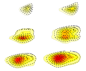
Contour plot of mean velocity $U/U_\infty$ from DNS. Dashed and dotted lines correspond to $\delta _{99}$ and $2\delta _{99}$, respectively. Marked squares in black represent the interrogation windows considered.

Consistent with Nolan & Walsh (Reference Nolan and Walsh2012) and Balamurugan & Mandal (Reference Balamurugan and Mandal2017), both $C_{{u^{\ast }u}}$ and $C_{{v^{\ast }v}}$ maps have their maxima at the location of the reference signal location since the time lag between the two signals is zero. However, one may observe that the $C_{{v^{\ast }u}}$ map has a negative minimum inside the BL, which simply indicates that a vertical perturbation towards the wall at the reference location directly induces a positive velocity perturbation inside the BL. Hence next, the spatial development of $C_{{v^{\ast }u}}$ is examined in both the streamwise and wall-normal directions. The interrogation windows investigated are shown in the contour plot of $U/U_\infty$ in figure 18.

For simplicity, the focus will first be on the three windows denoted A, B and C in figure 18. In all the contour maps of $C_{{v^{\ast }u}}$ displayed in figure 19, the dashed lines indicate the wall-normal locations of $y=\delta _{99}$. The wall-normal coordinates are normalized by corresponding BL thicknesses $\delta _{99}$, and $x$ coordinates are normalized by length scale $L$ (from DNS). The $v$ component of the velocity at the reference point (cross-marker outlined by a circle) is used to correlate the $u$ component of all the other spatial points to obtain the correlation maps. The minimum of $C_{{v^{\ast }u}}$ is highlighted as a filled white bullet. In addition, if only window A is considered, then the reference point is moving from $y/\delta _{99}=1.8$ (top) to 1.5 (middle), to 1 (lower). Moving downstream, i.e. from window A to window C, the physical distances from the BL edge to the reference points taken from window A are maintained constant.

Figure 19.

Two-point velocity correlation $C_{{v^{\ast }u}}$ maps from DNS. The dashed white line in each plot corresponds to $y=\delta _{99}$; the cross-marker outlined by the circle represents the reference point; a white circle represents the minimum value of $C_{{v^{\ast }u}}$. In each case from windows A to C, the reference point (cross-marker) is kept at the same physical distance above the BL edge.

Looking at window A with the reference location moving closer to the wall (from top to bottom) in figure 19, the magnitude of the peak minimum is increasing, and its location gradually moves closer to the wall. One may also observe a small upstream shift of this peak minimum. Regarding the positive maxima, it is of less interest since it is always located outside the BL, but it is also expected since a vertical perturbation towards the wall will slow down the streamwise velocity component and cause a negative perturbation and hence a positive correlation. Similar behaviour is visible in both windows B and C, which are located downstream of window A. It is noteworthy that the negative correlation value of $C_{{v^{\ast }u}}$ seems to be weakest in the intermediate window B. Moreover, the $y$ location of this minimum value consistently shifts towards the $\delta _{99}$ line going downstream from A to C. Here, the penetration depth $\varDelta _y$ is defined as the distance between $\delta _{99}$ and the location of the peak minimum in $C_{{v^{\ast }u}}$. It can be deduced that the normalized penetration depth $\varDelta _y/\delta _{99}$ can drop even though the physical penetration depth increases with the downstream direction since the BL grows. Note that in the DNS, since $y$ is normalized by the reference length $L$, $\varDelta _y$ is also normalized by $L$.

Figures 20(a,b) display the negative minimum value of $C_{{v^{\ast }u}}$ and the penetration depth $\varDelta _y$ as the reference $v^\ast$ signal moves away from the wall. As expected, both these quantities diminish for all windows, i.e. as a clockwise eddy moves away from the BL edge, the induced $u$ component inside the BL weakens, and the penetration naturally becomes shorter. In figure 20(c), only the reference signal at the BL edge, i.e. $y/\delta _{99}=1$, is considered. The FST penetration depth is plotted as its true value ($\varDelta _y$), normalized by local BL thickness ($\varDelta _y/\delta _{99}$) and integral length scale ($\varDelta _y/\varLambda _x$) versus the downstream distance. It is explicit that the true depth grows approximately 90 % from $Re_x = 0.3\times 10^5$ to $1.6\times 10^5$, and that it seems to scale with $\delta _{99}$, suggesting that the penetration depth is approximately 20 % of $\delta _{99}$. Since $\varLambda _x$ grows less than $\delta _{99}$ for this FST condition, the ratio $\varDelta _y/\varLambda _x$ grows slightly with the downstream distance. This can be an important result for future receptivity studies when the continuous FST forcing along the streamwise direction on the BL is compared with the LE receptivity.

Figure 20.

Minima of $C_{{v^{\ast }u}}$ and $\varDelta _y$ are plotted in (a,b) as a function of the reference signal location, respectively. (c) Downstream evolution of the penetration depth with the reference signal at the BL edge.