1 Introduction
Coherent structures within the turbulent boundary layer are known to be dominated by energetic large scales at high Reynolds numbers. They are populated in the outer region of the boundary layer and carry a significant portion of the turbulent kinetic energy, which contributes to almost half of the Reynolds shear stress in the boundary layer (Guala, Hommema & Adrian Reference Guala, Hommema and Adrian2006; Balakumar & Adrian Reference Balakumar and Adrian2007). These large-scale structures are also found to exhibit a footprint in the near-wall region affecting the near-wall structures (Hutchins & Marusic Reference Hutchins and Marusic2007a ). This has significant relevance in an engineering context since drag-reduction control strategies are usually based on manipulating the near-wall structures (Smits, McKeon & Marusic Reference Smits, McKeon and Marusic2011) and factors influencing these structures will have implications towards effective control strategies.
Bandyopadhyay & Hussain (Reference Bandyopadhyay and Hussain1984) examined the interaction between the large and small scales in various shear flows, including boundary layers, mixing layers, wakes and jets. They found significant coupling between these scales across all shear flows by correlating the low-frequency component (i.e. low-pass-filtered time-series data from hot-wire measurements) with a signal similar to the envelope of the high-frequency component. Later, Hutchins & Marusic (Reference Hutchins and Marusic2007a ) showed that the large scales tend to modulate the amplitude of the small-scale fluctuations. Mathis, Hutchins & Marusic (Reference Mathis, Hutchins and Marusic2009) expanded upon this nonlinear interaction and defined the modulation by a correlation coefficient between the large-scale streamwise fluctuating velocity and an envelope of the small-scale fluctuations to quantify the level of modulation across the boundary layer. Ganapathisubramani et al. (Reference Ganapathisubramani, Hutchins, Monty, Chung and Marusic2012), on the other hand, explored the dependence of the level of modulation on the strength of the large-scale fluctuations. In addition, they showed significant frequency modulation of the small-scale fluctuations by the large scales. Drawing from these studies, a predictive model for the near-wall turbulence was proposed with only large-scale information input (Marusic, Mathis & Hutchins Reference Marusic, Mathis and Hutchins2010; Mathis, Hutchins & Marusic Reference Mathis, Hutchins and Marusic2011a ).
The previous studies of Hutchins & Marusic (Reference Hutchins and Marusic2007a ) and Mathis et al. (Reference Mathis, Hutchins and Marusic2009, Reference Mathis, Hutchins and Marusic2011a ) consider canonical turbulent boundary layers, whereas Jacobi & McKeon (Reference Jacobi and McKeon2011a ,Reference Jacobi and McKeon b , Reference Jacobi and McKeon2013) and Duvvuri & McKeon (Reference Duvvuri and McKeon2015) introduced a synthetic large scale into the boundary layer to generalise the influence of large-scale structures on the small scales. Jacobi & McKeon (Reference Jacobi and McKeon2013) showed that very-large-scale motions are the primary modulating scale. Furthermore, Duvvuri & McKeon (Reference Duvvuri and McKeon2015) indicated that exciting the turbulent boundary layer by a large-scale input modifies the phase relationships naturally existing between the scales. These relationships are quantified by skewness and the amplitude modulation coefficient as previously suggested by Chung & McKeon (Reference Chung and McKeon2010) and later confirmed by Ganapathisubramani et al. (Reference Ganapathisubramani, Hutchins, Monty, Chung and Marusic2012). While the studies of Jacobi & McKeon (Reference Jacobi and McKeon2013) and Duvvuri & McKeon (Reference Duvvuri and McKeon2015) introduce a single large scale into the boundary layer, we input a wide range of large scales that are introduced from outside the boundary layer in the free stream. In this paper, we explore the effects of an external disturbance, namely free-stream turbulence (FST), on the turbulent boundary layer. Specifically, the focus is given towards the influence on the scale interactions.
FST exists above almost all naturally and industrially occurring turbulent boundary layers (Sharp, Neuscamman & Warhaft Reference Sharp, Neuscamman and Warhaft2009); therefore, in an engineering context, it is important to investigate how the turbulent boundary layer responds to FST. For the turbulent boundary layer, increased FST is widely known to cause increased skin friction and enhanced heat transfer (Blair Reference Blair1983; Hancock & Bradshaw Reference Hancock and Bradshaw1983; Castro Reference Castro1984). The focus of previous studies was to find parameters to correlate the increases of skin friction and heat transfer with FST. Hancock & Bradshaw (Reference Hancock and Bradshaw1983) concluded that the effect of FST was dependent not only on the turbulence intensity level but also on a characteristic length scale of FST, which they defined as the dissipation length scale. They formed an FST parameter using both the turbulence intensity and the length scale to define the overall effect of the FST on turbulent boundary layers. Blair (Reference Blair1983) added a damping term to this parameter to account for low-Reynolds-number effects. Later, Thole & Bogard (Reference Thole and Bogard1996) presented boundary layer statistics for FST levels up to
 $20\,\%$
and confirmed the validity of the log law in the mean profiles of the boundary layer for these high turbulence levels by direct measurements of total shear stress. Stefes & Fernholz (Reference Stefes and Fernholz2004) complemented the study of Thole & Bogard (Reference Thole and Bogard1996) by providing skin-friction data and measurements in the vicinity of the wall at relatively higher Reynolds numbers at FST levels up to
 $13\,\%$
. They also presented mean and fluctuating velocity distributions for the boundary layer and showed that there were considerable changes in the outer region of the boundary layer, such as the increase in the velocity fluctuations.
FST adds multiple length scales into the boundary layer and changes the nature of momentum and energy transport through scale interactions. Sharp et al. (Reference Sharp, Neuscamman and Warhaft2009) examined these scale interactions. They suggested that, depending on its level, FST can penetrate into the boundary layer as well as affect the small near-wall scales. However, the nearest wall-normal measurement location presented in their study is approximately
 $y^{+}\approx 50$
, where
 $y^{+}=yU_{\unicode[STIX]{x1D70F}}/\unicode[STIX]{x1D708}$
and
 $y$
is the wall-normal distance,
 $U_{\unicode[STIX]{x1D70F}}$
is the skin-friction velocity and
 $\unicode[STIX]{x1D708}$
is the kinematic viscosity. Therefore, the near-wall information is needed to establish a clear relationship between the near-wall turbulence and FST level and also to determine the extent of the FST penetration into the near-wall region. Currently, the mechanism on how FST interacts with the outer region of the boundary layer and how this in turn affects the near-wall turbulence, specifically in the context of scale interactions, is not well understood. With these motivations in hand, this paper aims to contribute towards the understanding of the scale interactions in a turbulent boundary layer in the presence of FST. Here we provide measurements of a turbulent boundary layer using hot-wire anemometry. The measurements could reach the wall down to
 $y^{+}\approx 5$
, which has the potential to reveal the near-wall information needed in the literature for a turbulent boundary layer under the effect of FST. The free stream is also characterised in detail by hot-wire measurements, and different FST conditions of increasing turbulence levels are investigated in detail in the paper.
2 Experiments
2.1 Facility
The experiments were performed in a suction-type wind tunnel at the University of Southampton. The test section of the tunnel is 4.5 m long and has a cross-section of
 $0.9~\text{m}\times 0.6~\text{m}$
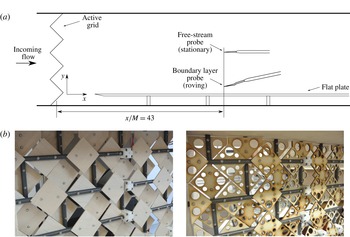
. A turbulent boundary layer was established on a 4.2 m long flat plate mounted 0.135 m above the floor of the test section. The plate had a sharp leading edge (machined from aluminium) that was followed by a Compocel® sandwich panel of parallel 1 mm thick aluminium sheets bonded to an 8 mm thick aluminium honeycomb core. A 0.5 m long flap followed at the trailing edge of the plate. The flap was used to position the stagnation point on the measurement side of the plate. The leading edge of the plate was positioned 0.3 m downstream of the active grid. The active grid was placed between the contraction and the test section of the tunnel. Although the grid-generated FST could trip the boundary layer to a turbulent state, the leading edge was also equipped with a tripping wire that was necessary for measurements made at low FST levels.
The design of the active grid used to generate the FST was based on that of Makita (Reference Makita1991) and similar later designs such as those found in Mydlarski & Warhaft (Reference Mydlarski and Warhaft1996), Kang, Chester & Meneveau (Reference Kang, Chester and Meneveau2003), Larssen & Devenport (Reference Larssen and Devenport2011) and Hearst & Lavoie (Reference Hearst and Lavoie2015). The active grid has a square mesh of length (
 $M$
) of 81 mm. To account for the rectangular test section, the active grid has
 $11\times 7$
rods, each with a diameter of 10 mm. Square wings of length 55.86 mm are attached to the rods, as shown in figure 1(b). Two sets of square wings have been used: one solid set and the other of the same outer dimension but with reduced solidity using circular cut-outs (see figure 1(b), left and right, respectively). The maximum frontal blockage by the solid wings is 100 % and this has been reduced to 75 % for the circular cut-out wings. Each of the rods could be rotated independently using stepper motors. The motors were daisy-chained and controlled through a Matlab routine. By using a combination of different rotational schemes and free-stream velocities
 $U_{0}$
, and with the two different sets of wings, a wide range of FST cases was possible. The turbulence intensity levels considered ranged from approximately 7 % to 13 %.
(a) Schematic of the test section. (b) Different sets of wings used during the experiment: solid wings (left) and cut-out wings (right).

2.2 Experimental methods
Measurements of the streamwise flow velocity in the boundary layer and in the free stream were made using two single-component hot-wire anemometers. Each hot-wire probe was located at the mid-span of the boundary layer plate and
 $43M$
downstream of the active grid. One probe was held stationary at 27 cm above the flat plate in the free stream, whereas the other could be traversed from the wall,
 $y=0$
, to the free stream, as shown in figure 1(a). The single wire traversing the boundary layer was an Auspex A55P05 boundary layer probe that had 10 mm long prongs spanned by a 3 mm long and
 $5~\unicode[STIX]{x03BC}\text{m}$
diameter tungsten wire with a central 1.05 mm active region shouldered on either side by copper-plated sections. The single wire located in the free stream was an Auspex A55P01 probe with the same active sensor length as the boundary layer probe. The resulting length-to-diameter ratio of each probe was 210, following the recommendation by Ligrani & Bradshaw (Reference Ligrani and Bradshaw1987) and Hutchins et al. (Reference Hutchins, Nickels, Marusic and Chong2009). A Dantec StreamLine Pro Constant Temperature Anemometer (CTA) system was used to operate the hot-wire probes with an overheat ratio set to 1.8. The output of the CTA system was low-pass-filtered at 10 kHz and was sampled at a rate of 20 kHz, to prevent aliasing, by a 16-bit National Instruments USB-6212 BNC analogue-to-digital data acquisition board, connected to a PC. Measurements of the streamwise velocity in the boundary layer were acquired at 28 wall-normal locations for a sampling period of 6 minutes. The streamwise velocity in the free stream was acquired simultaneously. The hot wires were statically calibrated using a 14-point velocity calibration ranging between 1.4 and
 $14~\text{m}~\text{s}^{-1}$
. The reference velocity was determined using a Pitot static tube connected to a Furness FCO510 0–200 Pa pressure transducer. The temperature of the free stream was acquired by a T-type Omega thermocouple throughout the experiments. Although the ambient temperature variation remained within
 $\pm 0.9\,^{\circ }\text{C}$
, the hot-wire output signals were corrected with respect to the reference temperature of the calibration (see Bruun Reference Bruun1995). Regardless, calibrations were performed immediately before (pre-) and after (post-) each experiment to linearly correct for drift between pre- and post-calibrations. The calibrations were performed while the wings of the grid were aligned with the free-stream direction, i.e. similar to a static mesh grid having turbulence levels of approximately 2 %–2.5 %. This calibration method was validated against a test with the grid removed and agreed within
 $\pm 1\,\%$
. Therefore, calibrations in all experiments reported were performed without removing the active grid.
The friction velocity was measured using the Preston tube method. For this method, the pressure difference was measured between two tubes: one is placed in contact with the wall and is open to the oncoming flow, whereas the other is a static pressure port drilled through the surface of the plate at the same streamwise location. This pressure difference was measured using a Furness FCO510 0–200 Pa pressure transducer. The total pressure tube was given a minor curvature and fixed with tape at the centre of its 15 cm length to ensure that the tube opening was in contact with the plate at all times. The tube placed in contact with the wall had a diameter of 2.76 mm and the static port diameter was 1 mm. This method is dependent on the assumption of the log-law validity (Patel Reference Patel1965), which will be shown to be valid for the boundary layers considered in this study. This method also required a calibration relating friction velocities derived from the log law to the difference between the total pressure measured by the Preston tube and the static pressure measured from the static port. For this calibration,
 $U_{\unicode[STIX]{x1D70F}}$
was measured using the Clauser chart method for the no-FST case over a range of
 $Re_{\unicode[STIX]{x1D70F}}$
that corresponded to the range of measured FST cases during the course of this study. Then, an in-house calibration was devised to relate these
 $U_{\unicode[STIX]{x1D70F}}$
values to the pressure differences measured simultaneously using Preston tubes. We have found excellent agreement (within the experimental uncertainty) with our own calibration and the calibration by Patel (Reference Patel1965) for Preston tube measurements. The results from the Preston tube were also validated by oil-film interferometry measurements, which were carried out later under the same conditions.
Free-stream parameters for the study cases at
 $x=43M$
:
 $U_{0}$
, mean streamwise velocity;
 $\sqrt{\overline{u_{0}^{2}}}/U_{0}~(\%)$
, turbulence intensity;
 $Re_{\unicode[STIX]{x1D706}_{0}}$
, Reynolds number based on the Taylor microscale;
 $L_{0}/M$
and
 $L_{0}^{\ast }/M$
, integral length scale ratios based on
 $M$
;
 $\unicode[STIX]{x1D706}_{0}$
, Taylor microscale;
 $\unicode[STIX]{x1D702}_{0}$
, Kolmogorov scale. Detailed definitions of the parameters are given in the text.

3 Results
3.1 Free-stream conditions
The FST cases were generated using the active grid by rotating the shafts at specified rotation rates during specified periods. Two different sets of wings, i.e. solid wings and cut-out wings, were used as described previously to achieve a range of turbulence intensity values from approximately 7 % to 13 %. The motor schemes of the active grid were reproduced from various active grid studies in the literature (Kang et al. Reference Kang, Chester and Meneveau2003; Larssen & Devenport Reference Larssen and Devenport2011). A total of 20 FST cases were documented during the course of this study (see table 1 and table 3 in the Appendix). Detailed analysis is generally limited to only the four cases given in table 1 for the sake of brevity and because the phenomena of interest to this study can be adequately described from this reduced set. However, we include trends determined from the inclusive set of 20 cases when broader points are made. For the cases investigated in detail (given in table 1) the operation parameters of the active grid were reproduced from Larssen & Devenport (Reference Larssen and Devenport2011) (test case 14 in their study). It involves setting a uniformly distributed rotational speed in the range of 2–6 Hz for each rod’s motor once every second while adjacent motors rotate in the opposite direction.
The characteristics of the four FST cases investigated in this paper are summarised in table 1. Using the solid or reduced blockage sets of wings mainly resulted in different levels of turbulence intensity. Cases A and B were generated using cut-out wings, resulting in what we will refer to as ‘low-range’ turbulence intensity levels of approximately 7–8 %. Cases C and D were generated using solid wings, resulting in what we will refer to similarly as ‘high-range’ turbulence intensity levels of approximately 12–13 %. The parameters are obtained from the measurements acquired at
 $43M$
downstream of the grid. The subscript 0 is used to denote the free-stream values throughout the paper. Quantities with this subscript were obtained from the stationary probe in the free stream. The instantaneous velocity in the streamwise direction is denoted by the sum of the mean and fluctuating components,
 $U+u$
. The Reynolds number
 $Re_{\unicode[STIX]{x1D706}_{0}}$
based on the Taylor microscale
 $\unicode[STIX]{x1D706}_{0}$
is defined as
 $\sqrt{\overline{u_{0}^{2}}}\unicode[STIX]{x1D706}_{0}/\unicode[STIX]{x1D708}$
, where
 $\unicode[STIX]{x1D706}_{0}$
is calculated as
 $\sqrt{(15\unicode[STIX]{x1D708}\overline{u_{0}^{2}}/\unicode[STIX]{x1D716})}$
. Within this definition, the turbulence energy dissipation rate
 $\unicode[STIX]{x1D716}$
is calculated from the spatial gradient of the streamwise velocity fluctuations as
 $15\unicode[STIX]{x1D708}\overline{(\unicode[STIX]{x2202}u_{0}/\unicode[STIX]{x2202}x)^{2}}$
, the formulation of which invokes Taylor’s hypothesis to obtain the spatial gradient from the temporal gradient calculated from the hot-wire measurements. To improve the estimate of the gradient quantities in a turbulent flow from hot-wire measurements, higher-order differencing schemes are suggested (Hearst et al.
Reference Hearst, Buxton, Ganapathisubramani and Lavoie2012); therefore seven-point centred differencing schemes were employed in this study to calculate the velocity gradients. Using the dissipation rate
 $\unicode[STIX]{x1D716}$
, the Kolmogorov scale (
 $\unicode[STIX]{x1D702}_{0}$
) can be calculated from
 $(\unicode[STIX]{x1D708}^{3}/\unicode[STIX]{x1D716})^{1/4}$
. There are several ways to define the integral length scale (
 $L_{0}$
) in a turbulent flow. A common definition is to use the value of the integrated normalised autocorrelation to the first zero crossing. However, it was found that the low-frequency energy content caused by the active grid prevented the autocorrelation from reaching zero. For this reason, a value of 0.1 was chosen in the present study to determine the extent of the integration region, which was above the asymptotic limit reached in all cases. Another common method to calculate the integral length scale often used in active grid studies is from the wavenumber at which the pre-multiplied spectra peak. Since this method is associated with significant scatter, Mydlarski & Warhaft (Reference Mydlarski and Warhaft1996) introduced the relation
 $L_{0}^{\ast }=0.9\overline{u_{0}^{2}}/\unicode[STIX]{x1D716}$
. The integral length scale using each of the aforementioned methods is included in table 1 for comparison purposes. As will become clear later, this study is particularly interested in the most energetic free-stream scales, which differ from the tabulated integral length scales.
The decay of turbulence downstream of a grid is governed by a power law as
 $\overline{u_{0}^{2}}/U_{0}^{2}=A(x/M)^{n}$
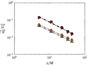
, as given in Mydlarski & Warhaft (Reference Mydlarski and Warhaft1996). For each of the four cases described in table 1, figure 2 shows the decay of the variance of streamwise velocity fluctuations,
 $\overline{u_{0}^{2}}$
. The measurements were performed along the test section midway between the test-section ceiling and the measurement side of the plate from approximately
 $x/M=5$
until the fixed downstream location for the boundary layer profiles,
 $x/M=43$
. For these cases, an exponent of
 $n=1.25$
adequately describes the observed decay shown in figure 2. This value is consistent with similar active grid studies from the literature (Mydlarski & Warhaft Reference Mydlarski and Warhaft1996; Kang et al.
Reference Kang, Chester and Meneveau2003). The vertical shift in figure 2 between the two different sets of lines, i.e. different constants of
 $A$
in the power-law equation, is caused by the solidity, i.e. the open area ratio, of the grid. Regardless, it can be deduced that the decay of turbulence is similar for each of the different FST cases. This suggests that the similarities and/or differences between different boundary layer cases presented in this study are not related to the rate of turbulence decay.
Decay of the normalised variance of the streamwise velocity fluctuations for the FST cases: filled triangle case A; filled diamond case B; filled right triangle case C; and filled square case D.

At the downstream location of the boundary layer profiles,
 $43M$
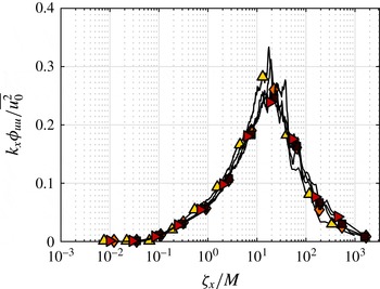
, figure 3 shows the pre-multiplied energy spectra of the streamwise velocity fluctuations in the free stream normalised by the local free-stream variance,
 $k_{x}\unicode[STIX]{x1D719}_{uu}/\overline{u_{0}^{2}}$
, with the streamwise wavelength
 $\unicode[STIX]{x1D701}_{x}$
normalised by the grid mesh length
 $M$
for the FST cases. The non-dimensional spectra are similar for each case and exhibit significant collapse. The characteristic wavelength of the spectral peak occurs at approximately
 $20M$
, which is several times longer than the integral length scales given in table 1. Given that the length scale of approximately
 $20M$
represents the most energetic scale, it is also chosen as the representative scale of turbulence in the free stream.
Normalised pre-multiplied energy spectra of streamwise velocity fluctuations,
 $k_{x}\unicode[STIX]{x1D719}_{uu}/\overline{u_{0}^{2}}$
, of the free stream for the FST cases versus streamwise wavelength
 $\unicode[STIX]{x1D701}_{x}$
of the free stream with respect to grid mesh length
 $M$
: filled triangle case A; filled diamond case B; filled right triangle case C; and filled square case D.

3.2 Boundary layer characteristics
A zero-pressure-gradient turbulent boundary layer was established under the influence of FST on a smooth flat plate as described previously in § 2.1. Herein, the characteristics of the turbulent boundary layers developed under the influence of different FST conditions, primarily those described in table 1 and with the inclusive dataset described in table 3 in the Appendix (where appropriate or relevant), will be discussed for the rest of the paper. In addition, in the instances where comparison is possible, they will be presented together with the baseline case taken without the presence of the active grid, which will be referred to as ‘no-FST’.
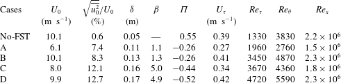
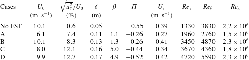
Table 2 is a summary of the turbulent boundary layer parameters for the no-FST case and for the four FST cases chosen for this paper. Table 2 is an extension of table 1 for the parameters of the boundary layers developed under the effect of the corresponding FST cases. The definitions of the parameters presented in table 2 are given in the following paragraphs.
There are several common approaches to define the thickness of the boundary layer. A common method is to report this thickness as the height at which the mean streamwise velocity in the boundary layer is equal to a fraction of the mean free-stream velocity, such as
 $\unicode[STIX]{x1D6FF}_{95}$
,
 $\unicode[STIX]{x1D6FF}_{99}$
or
 $\unicode[STIX]{x1D6FF}_{995}$
, corresponding to the height where the mean free-stream velocity reaches 95 %, 99 % or 99.5 % of
 $U_{0}$
, respectively. However, high fluctuations in the free stream due to the presence of the grid resulted in a wide scatter around the mean free-stream velocity, which could lead to the uncertainty associated with identifying the boundary layer thickness using these definitions. For this reason, the boundary layer thickness
 $\unicode[STIX]{x1D6FF}$
was defined using an integral method, which was found to be a more robust method for this study. The boundary layer thickness is calculated using the iterative integral method given by Perry & Li (Reference Perry and Li1990) as
 $\unicode[STIX]{x1D6FF}=\unicode[STIX]{x1D6FF}^{\ast }U_{0}/(C_{1}U_{\unicode[STIX]{x1D70F}})$
, where
 $\unicode[STIX]{x1D6FF}^{\ast }=\int _{0}^{\infty }(1-(U/U_{0}))\,\text{d}y$
is the displacement thickness,
 $C_{1}=\int _{0}^{1}((U_{0}-U)/U_{\unicode[STIX]{x1D70F}})\,\text{d}y/\unicode[STIX]{x1D6FF}$
and
 $U_{\unicode[STIX]{x1D70F}}$
is the skin-friction velocity obtained from Preston tube measurements. For a canonical boundary layer, this method results in typically 20 % higher
 $\unicode[STIX]{x1D6FF}$
values than that defined using
 $\unicode[STIX]{x1D6FF}_{99}$
(Perry & Li Reference Perry and Li1990).
Hancock & Bradshaw (Reference Hancock and Bradshaw1983) introduced the FST parameter,
 $\unicode[STIX]{x1D6FD}$
, defined as
 $(\sqrt{\overline{u_{0}^{2}}}/U_{0})/(L_{e}/\unicode[STIX]{x1D6FF}_{995}+2)$
, where the turbulence intensity
 $(\sqrt{\overline{u_{0}^{2}}}/U_{0})$
is given as a percentage and
 $L_{e}$
is a turbulence length scale defined from the decay power law of the grid turbulence (Castro Reference Castro1984). The purpose of this parameter is to account for the overall effect of FST by including the level of the turbulence and the characteristic length scale. Hancock & Bradshaw (Reference Hancock and Bradshaw1983) had a
 $\unicode[STIX]{x1D6FD}$
range of 0.62–1.72, Thole & Bogard (Reference Thole and Bogard1996) had a range of 2–4.6 and Sharp et al. (Reference Sharp, Neuscamman and Warhaft2009) presented results with
 $\unicode[STIX]{x1D6FD}$
values of 1.5 and 2.3. It should be noted that Thole & Bogard (Reference Thole and Bogard1996) used the
 $\unicode[STIX]{x1D6FF}_{99}$
definition instead of
 $\unicode[STIX]{x1D6FF}_{995}$
for the boundary layer thickness. Likewise, the present study invokes a different definition of the thickness, i.e. the
 $\unicode[STIX]{x1D6FF}$
definition given above, to calculate the
 $\unicode[STIX]{x1D6FD}$
values presented in table 2. The next tabulated parameter
 $\unicode[STIX]{x1D6F1}$
values represent the Coles wake parameter as defined by Coles (Reference Coles1956). Finally, the Reynolds numbers based on the skin-friction velocity
 $U_{\unicode[STIX]{x1D70F}}$
, the momentum thickness
 $\unicode[STIX]{x1D703}=\int _{0}^{\infty }(U/U_{0})(1-(U/U_{0}))\,\text{d}y$
and the streamwise distance
 $x$
are given in table 2 as
 $Re_{\unicode[STIX]{x1D70F}}=U_{\unicode[STIX]{x1D70F}}\unicode[STIX]{x1D6FF}/\unicode[STIX]{x1D708}$
,
 $Re_{\unicode[STIX]{x1D703}}=U_{0}\unicode[STIX]{x1D703}/\unicode[STIX]{x1D708}$
and
 $Re_{x}=U_{0}x/\unicode[STIX]{x1D708}$
, respectively.
Turbulent boundary layer parameters for FST cases at
 $x=43M$
, with the baseline no-FST case:
 $U_{0}$
, mean streamwise velocity of the free stream;
 $\sqrt{\overline{u_{0}^{2}}}/U_{0}~(\%)$
, FST intensity;
 $\unicode[STIX]{x1D6FF}$
, boundary layer thickness;
 $\unicode[STIX]{x1D6FD}$
, Hancock & Bradshaw (Reference Hancock and Bradshaw1983) FST parameter;
 $\unicode[STIX]{x1D6F1}$
, Coles wake parameter;
 $U_{\unicode[STIX]{x1D70F}}$
, skin-friction velocity;
 $Re_{\unicode[STIX]{x1D70F}}$
, Reynolds number based on skin-friction velocity;
 $Re_{\unicode[STIX]{x1D703}}$
, Reynolds number based on momentum thickness;
 $Re_{x}$
, Reynolds number based on streamwise distance. Detailed definitions of the parameters are given in the text.
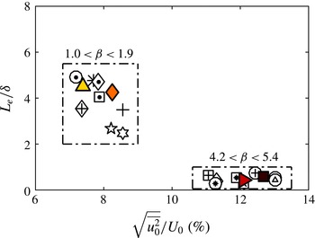
Turbulence length scale ratio defined by Hancock & Bradshaw (Reference Hancock and Bradshaw1983) with FST turbulence level: filled triangle case A; filled diamond case B; filled right triangle case C; and filled square case D. Conditions of the cases for all other data markers can be found in table 3 in the Appendix.

Parameter ranges. Plots of (a)
 $Re_{\unicode[STIX]{x1D70F}}$
versus
 $Re_{\unicode[STIX]{x1D706}_{0}}$
and (b)
 $Re_{\unicode[STIX]{x1D703}}$
versus turbulence intensity level (
 $\sqrt{\overline{u_{0}^{2}}}/U_{0}~(\%)$
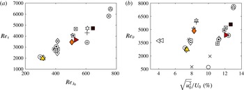
): filled triangle case A; filled diamond case B; filled right triangle case C; and filled square case D. Previous studies plotted in panel (b): open left triangle Hancock & Bradshaw (Reference Hancock and Bradshaw1983), open circle Thole & Bogard (Reference Thole and Bogard1996), cross Sharp et al. (Reference Sharp, Neuscamman and Warhaft2009). Conditions of the cases for all other data markers can be found in table 3 in the Appendix.

A length scale ratio (
 $L_{e}/\unicode[STIX]{x1D6FF}$
), originally proposed by Hancock & Bradshaw (Reference Hancock and Bradshaw1983) (albeit using
 $\unicode[STIX]{x1D6FF}_{995}$
), is defined for the FST cases. Figure 4 shows this length scale ratio with respect to the FST intensity. This plot and subsequent parameter plots are populated with the inclusive dataset summarised by table 2 and table 3 in the Appendix to reveal the trends (or lack of) between the relevant parameters. Referring back to figure 4, the cases can be grouped in two different
 $\unicode[STIX]{x1D6FD}$
ranges, which is mainly dependent on the wing type used. The four cases given in table 2 are chosen to be representative of these two distinct groups.
The extent of the parameter domain for
 $Re_{\unicode[STIX]{x1D706}_{0}}$
,
 $Re_{\unicode[STIX]{x1D70F}}$
and
 $Re_{\unicode[STIX]{x1D703}}$
is shown in figure 5. Referring to figure 5(a),
 $Re_{\unicode[STIX]{x1D70F}}$
appears to linearly increase with
 $Re_{\unicode[STIX]{x1D706}_{0}}$
. It must be noted that, although a distributed range of
 $Re_{\unicode[STIX]{x1D706}_{0}}$
has been obtained in the experiments, the range of turbulence intensities that were achieved is more clustered. This is primarily because the turbulence intensity values were related to the solidity of the wings of the active grid, as previously discussed. However, the variation of the Taylor microscale appears to be dependent on the actuation scheme of the active grid. Regardless, the approximate linear relationship between
 $Re_{\unicode[STIX]{x1D706}_{0}}$
and
 $Re_{\unicode[STIX]{x1D70F}}$
is reasonably clear from figure 5(a). The four cases chosen for this paper (table 2) also well manifest this linear relationship. It should also be noted that the
 $Re_{\unicode[STIX]{x1D70F}}$
range covered for the present study is not as wide as desired. Figure 5(b) shows the relationship between the turbulence intensity of the free stream (
 $\sqrt{\overline{u_{0}^{2}}}/U_{0}~(\%)$
) and
 $Re_{\unicode[STIX]{x1D703}}$
. Figure 5(b) shows that, for each of the low- and high-range FST groups,
 $Re_{\unicode[STIX]{x1D703}}$
increases with the level of FST. However, comparing the two different groups, a similar range of
 $Re_{\unicode[STIX]{x1D703}}$
is observed, although the level of FST is markedly different. This suggests that similar boundary layer characteristics may be developed under the effect of different FST levels and characteristics, which is further supported by the inclusion of several relevant examples from the literature. It can also be seen that the present study achieves higher
 $Re_{\unicode[STIX]{x1D703}}$
values with higher turbulence levels compared to those previous studies.
Development of boundary layer parameters. (a) Shape factor (
 $H$
) with
 $Re_{\unicode[STIX]{x1D703}}$
and (b)
 $Re_{\unicode[STIX]{x1D703}}$
with
 $Re_{x}$
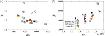
: filled triangle case A; filled diamond case B; filled right triangle case C; and filled square case D. No-FST case (open down triangle) and relevant data from Hancock & Bradshaw (Reference Hancock and Bradshaw1983) (open left triangle) are also plotted in panel (a). Conditions of the cases for all other data markers can be found in table 3 in the Appendix.

The shape factor,
 $H=\unicode[STIX]{x1D6FF}^{\ast }/\unicode[STIX]{x1D703}$
, is relevant to the evolution of the boundary layer and is a measure of the ‘fullness’ of the boundary layer. Owing to penetration of FST and therefore mixing in the boundary layer, there is higher momentum flux towards the wall and this increases the fullness of the velocity profile. That in turn means a decrease in the shape factor
 $H$
, as also shown in various previous studies (Hancock & Bradshaw Reference Hancock and Bradshaw1983; Castro Reference Castro1984; Stefes & Fernholz Reference Stefes and Fernholz2004; Brzek et al.
Reference Brzek, Torres-Nieves, Lebrón, Cal, Meneveau and Castillo2009). This is demonstrated in figure 6(a), which shows that the shape factor is reduced by the presence of FST in comparison to the no-FST case, which exhibits a typical value of approximately 1.4 for a turbulent boundary layer. Furthermore, the high-range turbulence intensity cases, i.e. cases with solid wings, typically have even lower values of
 $H$
compared to the low-range turbulence intensity cases, i.e. cases with cut-out wings. This suggests that there is higher FST penetration into the boundary layer for the higher turbulence intensity cases. The data of Hancock & Bradshaw (Reference Hancock and Bradshaw1983), which have low turbulence intensity of approximately 3–4 % generated by a static grid, are also shown in figure 6(a). The shape factors of their cases reside between the no-FST case and those of the comparatively higher FST cases of the present study, which supports the systematic reduction of the shape factor with increase in FST level. Furthermore, it is known that
 $H$
is a slowly decreasing function of
 $Re_{\unicode[STIX]{x1D703}}$
for a canonical turbulent boundary layer (Monkewitz, Chauhan & Nagib Reference Monkewitz, Chauhan and Nagib2008) and this observation also appears to be valid for the FST cases shown in figure 6(a).
Thus far, we have shown data that demonstrate the variation of different boundary layer parameters with different FST conditions. The aforementioned results were obtained by altering the velocity of the free stream, the active grid actuation scheme and its blockage. However, in order to examine the development of the boundary layer, it is perhaps more relevant to compare the state of the boundary layer at a fixed unit Reynolds number. In order to compare this, the boundary layer state (in this case
 $Re_{\unicode[STIX]{x1D703}}$
) is plotted against the Reynolds number based on the downstream distance of the test plate,
 $Re_{x}$
, in figure 6(b). This representation takes into account the decay of the FST and the growth of the boundary layer in some ways and can be used to compare cases at the same
 $Re_{x}$
for different intensity values of FST. If the power-law decay rate of the FST is the same across different cases (as previously shown), then this plot shows the development of the boundary layer up to a fixed value of
 $Re_{x}$
. Figure 6(b) shows that, for the same
 $Re_{x}$
(indicated by dashed arrows in the direction of increasing turbulence intensity), higher turbulence intensity in the free-stream results in higher
 $Re_{\unicode[STIX]{x1D703}}$
. It can also be observed that one could change
 $Re_{x}$
and obtain the same
 $Re_{\unicode[STIX]{x1D703}}$
by modifying the FST intensity. It should be noted that the four FST cases given in table 2 enable the comparison of the effects of different FST levels on the boundary layer for a fixed
 $Re_{x}$
, say cases B and D, and the effects of different
 $Re_{x}$
for similar FST levels, say cases A and B and/or cases C and D.
Variation of skin-friction coefficient
 $C_{f}$
with
 $Re_{\unicode[STIX]{x1D703}}$
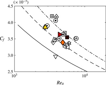
: filled triangle case A; filled diamond case B; filled right triangle case C; and filled square case D. Also plotted are: open down triangle no-FST case; open left triangle Hancock & Bradshaw (Reference Hancock and Bradshaw1983); (——) Fernholz & Finley (Reference Fernholz and Finley1996) correlation; and (- - - -) fitted line for low-range turbulence intensity cases and (–.) fitted line for high-range turbulence intensity cases based on Fernholz & Finley (Reference Fernholz and Finley1996) correlation. Conditions of the cases for all other data markers can be found in table 3 in the Appendix.

It has been well established that the presence of FST increases the skin friction in the boundary layer (Blair Reference Blair1983; Hancock & Bradshaw Reference Hancock and Bradshaw1983; Castro Reference Castro1984; Stefes & Fernholz Reference Stefes and Fernholz2004). For a smooth-wall zero-pressure-gradient boundary layer without FST, the skin-friction coefficient is given as a function of Reynolds number,
 $Re_{\unicode[STIX]{x1D703}}$
, through a semi-empirical relation by Fernholz & Finley (Reference Fernholz and Finley1996). The baseline case from this study is captured by their relation, as shown in figure 7, whereas the FST cases result in larger values of the skin-friction coefficient compared to this relation. Figure 7 also appears to show that the empirical relation of Fernholz & Finley (Reference Fernholz and Finley1996) seems to hold for the FST cases, however, with different offset values for the two different turbulence ranges shown in the plot as fitted lines. At a constant
 $Re_{\unicode[STIX]{x1D703}}$
of, say, 6000 from figure 7, where there are data for three different turbulence intensities (one of Hancock & Bradshaw (Reference Hancock and Bradshaw1983) and two of the present study cases of low- and high-range turbulence), it can be seen that an increase in the FST intensity causes an increase in the skin-friction coefficient.
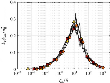
The preceding analysis demonstrated the significance of FST on the properties of the boundary layer. We now consider outer-variable scaling of the free-stream velocity fluctuations, since the boundary layer thickness and the FST appeared to be coupled (see table 2). Figure 8 shows the pre-multiplied energy spectra of the streamwise velocity fluctuations in the free stream normalised by local free-stream variance,
 $k_{x}\unicode[STIX]{x1D719}_{uu}/\overline{u_{0}^{2}}$
. The streamwise wavelength,
 $\unicode[STIX]{x1D701}_{x}$
, appears on the abscissa normalised by
 $\unicode[STIX]{x1D6FF}$
. Each case appears to be forced from the free stream at a similar length scale of approximately
 $10\unicode[STIX]{x1D6FF}$
. This suggests that the external disturbance experienced by the boundary layer is most energetic at approximately
 $10\unicode[STIX]{x1D6FF}$
and the response to forcing at this dominant scale for different levels of forcing (i.e. FST level) can be examined in detail by comparing the boundary layer subjected to these different cases. The following sections will examine the influence of FST on the statistical as well as the spectral characteristics of a turbulent boundary layer.
Normalised pre-multiplied energy spectra of streamwise velocity fluctuations,
 $k_{x}\unicode[STIX]{x1D719}_{uu}/\overline{u_{0}^{2}}$
, of the free stream for the FST cases with streamwise wavelength,
 $\unicode[STIX]{x1D701}_{x}$
, of the free stream with respect to boundary layer thickness,
 $\unicode[STIX]{x1D6FF}$
: filled triangle case A; filled diamond case B; filled right triangle case C; and filled square case D.

3.3 Mean velocity
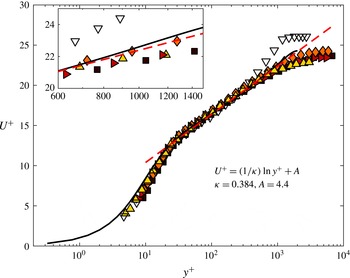
The inner-normalised mean streamwise flow velocity is shown in figure 9 for the study cases together with the baseline case. The skin-friction velocity in all cases was determined using the Preston tube method. A remarkable feature of the mean velocity profiles of turbulent boundary layers subjected to FST is the persistence of the log-law region for FST levels up to 20 % (Thole & Bogard Reference Thole and Bogard1996). The inner-scaled profiles (figure 9) here also confirm the validity of the log law. It shows a clear collapse below the outer region with log-law coefficients of von Kármán constant
 $\unicode[STIX]{x1D705}=0.384$
and constant
 $A=4.4$
; these coefficient values follow from Marusic et al. (Reference Marusic, Monty, Hultmark and Smits2013). This suggests that the effect of FST on the mean flow in the inner region is to alter the value of the skin-friction velocity. However, once this change is accounted for, there is self-similarity in the logarithmic region and below. This indicates a proportional effect of the FST in the mean flow and robustness of the law of the wall even when subjected to large external disturbances. This collapse in the mean profiles has also been interpreted by Hancock & Bradshaw (Reference Hancock and Bradshaw1989) as the mean flow being less affected by FST. The mean velocity profiles deviate from similarity to the baseline no-FST case as the FST cases have an extended logarithmic region compared to the no-FST case. From figure 9, the deviation point of the profiles from the log law is obvious for the no-FST case, whereas for the FST cases deviation from that curve occurs at much higher wall-normal positions (in wall units), therefore implying an extended region that is defined by the logarithmic law. The inset in figure 9 shows a close-up view of the profiles, which highlights the similar extension of the logarithmic region for the FST cases. Within the measurement uncertainty, the profiles exhibit a logarithmic region that extends up to
 $y^{+}\approx 700$
. This has important implications for the overlap region argument of the turbulent boundary layer. It can be deduced that the validity of the law of the wall, i.e.
 $U^{+}=f(y^{+})$
, is not dictated here by the outer scales in the boundary layer, and FST can be said to affect these outer scales in such a way that the law of the wall can extend up to higher wall-normal positions in wall units. It is assumed for a canonical turbulent boundary layer that the logarithmic law is valid up to
 $y^{+}=0.2Re_{\unicode[STIX]{x1D70F}}$
; therefore, looking at the extended
 $y^{+}$
values from figure 9, a Reynolds-number analogy between the present FST cases and canonical boundary layers can be made. This would imply that the present FST cases represent a high-Reynolds-number flow without FST at
 $Re_{\unicode[STIX]{x1D70F}}$
of approximately 3500.
Inner-normalised mean velocity profiles: filled triangle case A; filled diamond case B; filled right triangle case C; and filled square case D; open down triangle no-FST case; (- - - -) log law with coefficients
 $\unicode[STIX]{x1D705}=0.384$
and
 $A=4.4$
; (——) DNS channel flow data at
 $Re_{\unicode[STIX]{x1D70F}}\approx 2000$
from Hoyas & Jiménez (Reference Hoyas and Jiménez2006). The inset shows a close-up of the profiles for the range of
 $600<y^{+}<1500$
.

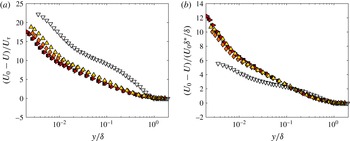
Velocity defect profiles normalised by (a) inner velocity scaling and (b) outer velocity scaling proposed by Zagarola & Smits (Reference Zagarola and Smits1998): filled triangle case A; filled diamond case B; filled right triangle case C; filled square case D; and open down triangle no-FST case.

The extension of the logarithmic region is intimately connected to the suppression of the wake region under the effect of FST. In a canonical boundary layer like the no-FST case, the profile is bounded by the onset of intermittency resulting in a well-defined wake region; however, for a turbulent boundary layer under the FST effect, there is no intermittent region since the free stream is also turbulent and thus the wake region almost vanishes. For this reason, turbulent boundary layers under the FST effect can be said to have similarities with a turbulent channel flow where there is significant turbulence in the outer region at the centreline of the channel. Direct numerical simulation (DNS) data of a turbulent channel flow at
 $Re_{\unicode[STIX]{x1D70F}}\approx 2000$
from Hoyas & Jiménez (Reference Hoyas and Jiménez2006) have been added on the mean profile plot for comparison. The suppression of the wake region with respect to the no-FST case is also obvious from their data and shows similarities to the present FST cases. This lack of a wake in the channel is primarily due to the presence of a turbulent core. In addition to a turbulent core, the presence of a favourable pressure gradient (FPG) in channel flows would also tend to suppress the wake region (Nagib & Chauhan Reference Nagib and Chauhan2008); however, this pressure gradient effect is likely to be weak especially at higher Reynolds number. Having said that, the presence of an FPG will indeed reduce the wake strength in external flow (i.e. boundary layers) due to the acceleration of the free stream. In fact, Stefes & Fernholz (Reference Stefes and Fernholz2004) made an analogy between the FST effect on the wake region of the turbulent boundary layer and the effect of an FPG on a turbulent boundary layer. Consequently, external flows with an FPG such as sink flows (Jones, Marusic & Perry Reference Jones, Marusic and Perry2001) can also produce a mean flow that is similar to the ones presented in the current study; however, the turbulence properties are likely to be different.
The velocity defect profiles in two different scalings are given in figure 10. The suppression of the wake region can be clearly observed from both scalings. For the first scaling shown in figure 10(a), the velocity defect is either very small or absent in the outer region of the boundary layer when compared with the no-FST case. This results in reduced wake strength, as expected for a turbulent boundary layer under the effect of FST (Thole & Bogard Reference Thole and Bogard1996; Sharp et al.
Reference Sharp, Neuscamman and Warhaft2009). Correspondingly, the Coles wake parameter
 $\unicode[STIX]{x1D6F1}$
that quantifies the wake strength reduces in the presence of FST and even becomes negative for strong FST cases, as shown in table 2. In figure 10(b), the outer velocity scale proposed by Zagarola & Smits (Reference Zagarola and Smits1998) is considered following the observations by Brzek et al. (Reference Brzek, Torres-Nieves, Lebrón, Cal, Meneveau and Castillo2009). Although the scaling effectively removes Reynolds-number variations in the mean velocity defect law for various flows (Klewicki Reference Klewicki2010), it has been shown by Brzek et al. (Reference Brzek, Torres-Nieves, Lebrón, Cal, Meneveau and Castillo2009) that it does not completely eliminate the effects of high FST. Therefore, the Zagarola & Smits scaling does not offer any improvement compared to inner scaling for the velocity defect similarity of the FST cases with respect to the no-FST case; however, the various FST cases appear to collapse. This scaling is proportional to the mass flux deficit, i.e.
 $\unicode[STIX]{x1D6FF}^{\ast }$
, and, since the mass flux deficit does not vary among different FST cases, the similarities between different cases can therefore be justified. Although Brzek et al. (Reference Brzek, Torres-Nieves, Lebrón, Cal, Meneveau and Castillo2009) observed an improved collapse with the Zagarola & Smits scaling, an overall collapse as shown in figure 10(b) was not achieved. This is probably due to the fact that the mass flux in their case is also under the influence of surface roughness.
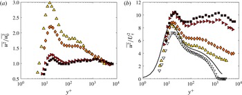
Variance profiles of streamwise velocity fluctuations, (a) free-stream variance-normalised and (b) inner-normalised: filled triangle case A; filled diamond case B; filled right triangle case C; and filled square case D. The no-FST case (open down triangle) and DNS channel flow data at
 $Re_{\unicode[STIX]{x1D70F}}\approx 2000$
from Hoyas & Jiménez (Reference Hoyas and Jiménez2006) (solid line) are also plotted in panel (b).

3.4 Streamwise broadband turbulence intensity and energy spectra
The broadband turbulence intensity, i.e. variance, profiles of the streamwise velocity fluctuations are given in figure 11 for two different normalisations. For the first case, the variance profiles are normalised by the corresponding variance of the free-stream fluctuations (figure 11
a). Within the boundary layer, the normalisation does not collapse these profiles. Rather, this normalisation may be interpreted as a gain of the turbulence level in the boundary layer compared to the FST whereby the turbulent fluctuations outside the boundary layer amplify the fluctuations within the boundary layer. Therefore, in the free stream the amplification is exactly
 $\overline{u^{2}}/\overline{u_{0}^{2}}=1$
. Within the boundary layer the amplification may vary up to the wall owing to the penetration of FST. Using this analogy, we can further say that the level of amplification and the distribution vary with the level of the free-stream disturbance. For example, it is shown in figure 11(a) that for higher turbulence levels a more uniform amplification throughout the boundary layer exists. In contrast, for the lower turbulence range, the near-wall turbulence peak remains a dominant feature. Therefore, the highest amplification probably occurs when the free stream is laminar and when the fluctuations in the near-wall region are governed solely by the near-wall cycle. This suggests a possible saturation limit for the turbulence within the boundary layer when subjected to external disturbances. Because a relative effect of the FST at each wall-normal location can be observed, the investigation of the energy distribution throughout the boundary layer with spectral analysis will be used to clarify how the energy of the FST affects the different regions of the boundary layer.
The inner-normalised variance profiles are presented in figure 11(b) in comparison with the no-FST case and with the DNS data from Hoyas & Jiménez (Reference Hoyas and Jiménez2006) for a turbulent channel flow. The response of the fluctuating component of the streamwise velocity in the boundary layer to the change in the FST level is not consistent, which is similarly found in figure 11(a). Immediately evident from figure 11(b) are the behaviour of the near-wall peak and the emergence of an outer peak for these laboratory-scale flows. In the following sections, we examine both these features in greater detail.
3.4.1 Near-wall region
For canonical turbulent boundary layers, the near-wall turbulence production, governed by the near-wall cycle of streaks and quasi-streamwise vortices, peaks at
 $y^{+}\approx 15$
as documented in many studies to date (Smits et al.
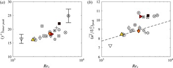
Reference Smits, McKeon and Marusic2011). In the present study, the location of the near-wall peak appears to propagate away from the wall (for inner scaling) with increasing Reynolds number, as shown in figure 12(a) for the inclusive dataset summarised in table 2 and in table 3 in the Appendix. The error bars represent the largest uncertainty in locating the wall to justify the discrepancy of the present cases from the expected
 $y^{+}\approx 15$
location. The outward movement of the near-wall peak, in wall units, has important implications in terms of the extent of the penetration and the governance of the near-wall turbulence production. Similar behaviour can be found in the comparable data shown by Stefes & Fernholz (Reference Stefes and Fernholz2004); however, they did not mention this gradual movement of the peak location. Regardless, the current study does not have a sufficient range of conditions to identify a definitive relationship between FST and the movement of the near-wall peak.
Variation of (a) the location and (b) the amplitude of the near-wall peak of the inner-normalised variance of the streamwise velocity fluctuations with Reynolds number: filled triangle case A; filled diamond case B; filled right triangle case C; filled square case D; and open down triangle no-FST case. Conditions of the cases for all other data markers can be found in table 3 in the Appendix. Error bars shown in panel (a) correspond to 10 % uncertainty in
 $y^{+}$
; dashed line in panel (b) is the curve fit,
 $(\overline{u^{2}}/U_{\unicode[STIX]{x1D70F}}^{2})_{peak}=1.036+0.965\ln (Re_{\unicode[STIX]{x1D70F}})$
, given by Hutchins & Marusic (Reference Hutchins and Marusic2007b
).

The near-wall peak amplitude increases with the turbulence intensity level of the free stream. Similar attributes in the near-wall peak are also encountered in high-Reynolds-number boundary layers for increasing Reynolds numbers,
 $Re_{\unicode[STIX]{x1D70F}}$
(Smits et al.
Reference Smits, McKeon and Marusic2011). For these types of flow, the energy in the outer region grows as the Reynolds number increases, implying that the fluctuations of the outer-region structures become stronger and comparable to the fluctuations of the near-wall structures (Hutchins & Marusic Reference Hutchins and Marusic2007a
). This induces a growing influence of the energetic outer region on the near-wall region and explains the increase in the near-wall peak amplitude. A possible analogy with high-Reynolds-number flows in this respect implies similar interactions between the structures of the near wall and the large structures in the outer region for the present FST cases. The difference here in this study compared to a high-Reynolds-number flow without FST is that the outer large scales here are introduced by large scales of the free stream that penetrate into the boundary layer. The trend in the near-wall peak amplitude for the FST cases is given in figure 12(b), which is again populated with the inclusive dataset summarised in table 2 and in table 3 in the Appendix. Also included is the relation given by Hutchins & Marusic (Reference Hutchins and Marusic2007b
) for the variation of the near-wall peak with
 $Re_{\unicode[STIX]{x1D70F}}$
. For low-range turbulence intensity cases, the data appear scattered about the relationship given by Hutchins & Marusic (Reference Hutchins and Marusic2007b
) whereas the high-range turbulence intensity cases appear consistently above that relation. Regardless, it is evident that for FST cases, like in high-Reynolds-number flows, the increase in the near-wall peak can also be attributed to the increasing influence of the large scales on the near-wall region as they become more energetic with increasing Reynolds number.
It is also worth mentioning that the increase in the fluctuation levels in the near-wall peak varies among the different cases. The difference in the peak levels with respect to the no-FST case is more prominent between the low- and high-range turbulence intensity cases (e.g. between cases B and D or between cases A and C) than between the similar intensity cases (e.g. between cases A and B or between cases C and D). This is due to higher penetration of FST into the boundary layer in higher FST cases, a point that will be made clear from examining the spectra. This also indicates that the increase in the level of fluctuations in the near-wall region is mostly governed by the level of turbulence in the free stream.
Figure 11(b) also shows that the near-wall peak for case A is similar to that of a turbulent channel flow at a comparable Reynolds number. However, the channel flow has an FST of only approximately 2 % (i.e. the streamwise turbulence intensity at the centreline of the channel). This indicates that, although the FST cases do not have an outer wake region in the mean flow due to loss of intermittency, analogous to the channel flow, a much higher FST appears to be necessary for the near-wall peak to have the same intensity as a channel flow at the same
 $Re_{\unicode[STIX]{x1D70F}}$
. This suggests that the near-wall region of the boundary layer damps out the outer disturbances much more than in a channel flow.
3.4.2 Outer region
The outer region of the boundary layer is directly affected by the presence of FST, in comparison to that of the near-wall region, as shown in figure 11(b). The variance of the no-FST case levels off at approximately zero since the free stream has near-zero turbulence whereas the FST cases level off at non-zero free-stream fluctuation values. For each of the FST cases, starting from the level of FST at the edge of the boundary layer, the fluctuations in the outer region are amplified. The amplification there appears higher for high-range turbulence intensity cases. This reflects the growing energy level in the free stream. Similarly, in high-Reynolds-number flows, the outer scales become more energetic as the Reynolds number increases and this is reflected in the emergence of an outer peak in the streamwise velocity spectra (Hutchins & Marusic Reference Hutchins and Marusic2007a ). Also, the increasing magnitude and constancy of the plateau-like region in the variance profiles is observed to coincide with that peak (Klewicki Reference Klewicki2010). Therefore, in an attempt to investigate the energy distribution for the present cases, spectral analysis is performed and interesting similarities with high-Reynolds-number flows are observed.
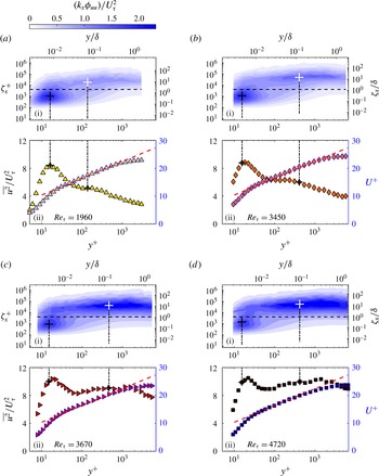
Figure 13 shows contour maps of the inner-normalised pre-multiplied energy spectra of the streamwise velocity fluctuations that are plotted against wall distance
 $y$
and streamwise wavelength
 $\unicode[STIX]{x1D701}_{x}~(=2\unicode[STIX]{x03C0}/k_{x})$
, for the FST cases with their corresponding mean velocity and variance profiles. Figure 13(a)–(d) are in order of increasing turbulence intensity levels. They are also in increasing order of friction Reynolds numbers, with
 $Re_{\unicode[STIX]{x1D70F}}=1960$
, 3450, 3670 and 4720, respectively. For each of the contour maps, two distinct peaks in the energy are observed, which will be referred to as the inner and outer spectral peaks and indicated by black and white
 $+$
symbols, respectively. The inner spectral peak corresponds to the near-wall cycle of streaks and quasi-streamwise vortices. The location of that peak is found to be fixed in inner coordinates at
 $y^{+}\approx 15$
and
 $\unicode[STIX]{x1D701}_{x}^{+}\approx 1000$
from all the spectral plots as also previously found in Hutchins & Marusic (Reference Hutchins and Marusic2007a
,Reference Hutchins and Marusic
b
) for a canonical turbulent boundary layer. The vertical dashed lines following the inner spectral peak also show the corresponding wall-normal location in variance profiles presented in plot (ii) for each case. As the FST level increases, it can be seen that the near-wall spectral peak remains rooted at
 $y^{+}=15$
. However, the near-wall broadband peak in the variance seems to move outwards, as observed previously in figure 12(a). The disparity between these two peak locations can be related to the low-wavenumber content of the FST in the near-wall region. The footprint of the outer broadband peak in the near-wall region is essentially causing the inner broadband peak to occur further away from the wall. Apart from indicating how far the penetration can go down to very near the wall, it can also be deduced that the extent of the penetration depends on the level of turbulence. This is consistent with the observed increase in the near-wall peak amplitude (figure 11
b) with increasing FST level.
(i) Contour maps of the inner-normalised pre-multiplied energy spectra of the streamwise velocity fluctuations,
 $k_{x}\unicode[STIX]{x1D719}_{uu}/U_{\unicode[STIX]{x1D70F}}^{2}$
, for: (a) case A filled triangle; (b) case B filled diamond; (c) case C filled right triangle; and (d) case D filled square. The ordinates show streamwise wavelength,
 $\unicode[STIX]{x1D701}_{x}$
, in both inner (left) and outer (right) scaling. The abscissas show the wall-normal location,
 $y$
, also plotted in both inner (bottom) and outer (top) scaling. The
 $+$
symbols indicate inner (black) and outer (white) spectral peaks. The horizontal dashed line represents the location of the cut-off wavelength at
 $\unicode[STIX]{x1D701}_{x}^{+}\approx 4000$
. (ii) Corresponding mean (blue outlined markers) and variance profiles. Dashed red line: log law with coefficients
 $\unicode[STIX]{x1D705}=0.384$
and
 $A=4.4$
. Dot-dashed vertical lines and the
 $+$
symbols represent the locations corresponding to the spectral peaks indicated on (i).

As mentioned previously, there is a second distinct spectral peak in the outer region indicated with a white
 $+$
symbol on spectral plots. The emergent outer spectral peaks for FST cases seem to increase in magnitude with increasing Reynolds number, i.e. with increasing FST levels. A similar behaviour is also known to occur for the canonical turbulent boundary layer with increasing Reynolds number. This similarity could have implications in mimicking high-Reynolds-number flows that are difficult to achieve without a purpose-built facility, by using FST with much lower Reynolds numbers.
For the high-range turbulence cases, two distinct broadband peaks are observed in the variance profiles; here, however, we focus on the peak that corresponds to a location inside the logarithmic region. The origin of the other broadband peak further from the wall would require a large database of high FST cases to give detailed consideration and it is therefore not discussed here. Within the logarithmic region, the broadband turbulence peak coincides with the plateau-like region in the variance profiles. For sufficiently high-Reynolds-number flows, i.e. having sufficient scale separation, the wall-normal location of that peak has been shown to nominally coincide with the centre of the log region as shown by Hutchins & Marusic (Reference Hutchins and Marusic2007a
). They also related the outer peak with the large-scale structures in the log region. For FST cases, a similar behaviour is observed where there appears to be a nominal spectral peak in the log region. Furthermore, the peak energy in this region occurs about a wavelength of
 $10\unicode[STIX]{x1D6FF}$
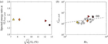
, which is also the most energetic wavelength in the free stream. This behaviour was also observed by Sharp et al. (Reference Sharp, Neuscamman and Warhaft2009) where they presented the pre-multiplied energy spectra of the boundary layer at different wall-normal locations and the free stream together and they concluded that the energetic wavelengths in the outer region were associated with the most energetic scales of the free stream. Given the relationship between the free-stream energetic scales and the outer spectral peak, we can look at the ratio of their corresponding spectral energies at the outer peak wavelength. In this way, we could obtain a wavelength-specific gain of the turbulence level compared to FST, as given in figure 14(a). This is similar to the broadband gain that is previously presented in figure 11(a). Likewise, it is deduced that the level of amplification varies with the level of the free stream and high-range FST cases tend to amplify less.
For canonical turbulent boundary layers, the location of the outer spectral peak has been shown to gradually move outwards in wall units,
 $y^{+}$
, with increasing
 $Re_{\unicode[STIX]{x1D70F}}$
and this movement is also found to be proportional to
 $Re_{\unicode[STIX]{x1D70F}}^{1/2}$
(Klewicki et al.
Reference Klewicki, Fife, Wei and McMurtry2007; Mathis et al.
Reference Mathis, Hutchins and Marusic2009). The location of the outer spectral peak for the inclusive set of FST cases shows agreement with this trend, as plotted in figure 14(b). Despite the good agreement, it should be noted that the range of
 $Re_{\unicode[STIX]{x1D70F}}$
covered in this study is limited and it is therefore very difficult to decipher this relationship without the guidance from previous work in this area.
(a) Spectral energy ratio between the FST and the boundary layer at the outer peak wavelength and (b) variation of the wall-normal location of the outer peak of the inner-normalised variance of the streamwise velocity fluctuations with Reynolds number: filled triangle case A; filled diamond case B; filled right triangle case C; and filled square case D. Conditions of the cases for all other data markers can be found in table 3 in the Appendix. The dashed line in panel (b) represents the relation
 $3.9Re_{\unicode[STIX]{x1D70F}}^{1/2}$
from Mathis et al. (Reference Mathis, Hutchins and Marusic2009) for the wall-normal location of the outer peak based on the definition of the log region as
 $100<y^{+}<0.15Re_{\unicode[STIX]{x1D70F}}$
.

3.5 Scale separation and amplitude modulation
Despite not having measurements very close to the wall, Sharp et al. (Reference Sharp, Neuscamman and Warhaft2009) suggested that the FST can reach deep into the boundary layer and have a direct effect on the inner scales of the boundary layer. The previous section demonstrated that the direct effect indeed reaches down to the wall and in fact moves the near-wall peak farther away from the wall. It is perhaps also important to examine any other effect of FST on near-wall turbulence. Decomposing the scales as large and small scales using a sharp spectral cut-off filter, Mathis et al. (Reference Mathis, Hutchins and Marusic2009) found that the near-wall turbulence is modulated by the energetic outer region of the flow in a canonical high-Reynolds-number boundary layer. We aim to carry out a similar analysis for the FST cases. A filter at a cut-off wavelength (
 $\unicode[STIX]{x1D701}_{x}^{+}$
) of 4000 (the horizontal dashed line in figure 13) represents a reasonable demarcation between the large- and small-scale components of the streamwise fluctuating velocity signal. This also corresponds to
 $\unicode[STIX]{x1D701}_{x}/\unicode[STIX]{x1D6FF}\approx 1{-}2$
for all the cases. The robustness of the decoupling procedure is shown in Mathis et al. (Reference Mathis, Hutchins and Marusic2009) for various different cut-off wavelengths; therefore, in terms of investigating the interactions between the large and small scales, the choice of cut-off wavelength is not expected to have a considerable effect.
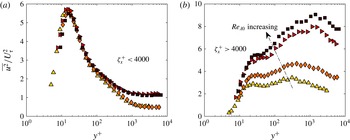
Variance profiles of scale-decomposed streamwise velocity fluctuations. (a) Small scales and (b) large scales based on a cut-off wavelength filter of
 $\unicode[STIX]{x1D701}_{x}^{+}=4000$
: filled triangle case A; filled diamond case B; filled right triangle case C; and filled square case D.

Figure 15 shows the inner-normalised variance profiles of scale-decomposed streamwise velocity fluctuations. These two separate variance profiles can be considered as the two components that add up to the variance profiles presented in figure 11(b). The contribution from the small scale to the total variance of the streamwise velocity fluctuations (figure 15 a) does not seem to change with different turbulence intensity levels across most of the boundary layer; however, overall, the effect of small scales seems to diminish to the edge of the boundary layer for all FST cases. The small-scale variance profiles have essentially eliminated any superposed effect of large-scale motions on the measured statistics. The fact that the small-scale contributions collapse for different cases after filtering out the superposition of large scales indeed confirms the direct penetration effect of FST on the near-wall region as also suggested by Sharp et al. (Reference Sharp, Neuscamman and Warhaft2009).
The large-scale variance profiles exhibit an increase in the near-wall region, reaching a local maximum (
 $y^{+}\approx 15{-}30$
), and increase further farther away from the wall. Overall, large-scale contribution increases across almost all wall-normal locations with increasing FST levels. Apart from gradual movement of the local peak turbulence intensity location, there is also amplitude increase of the local peak with increasing FST levels. This is also observed in high-Reynolds-number flows as the increasing effect of large scales on the near-wall region with increasing Reynolds number and this is found to be an indication of a growing outer-layer influence on the near-wall region (Hutchins & Marusic Reference Hutchins and Marusic2007b
; Smits et al.
Reference Smits, McKeon and Marusic2011).
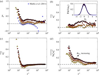
Variation of (a) the skewness factor
 $S_{u}$
, in comparison with the data from Mathis et al. (Reference Mathis, Hutchins and Marusic2009), and dominant terms of the scale-decomposed skewness (b)
 $\overline{\overline{{u_{L}^{+}}^{3}}}$
, (c)
 $\overline{\overline{{u_{S}^{+}}^{3}}}$
and (d)
 $3\overline{\overline{u_{L}^{+}{u_{S}^{+}}^{2}}}$
across the boundary layer: filled triangle case A; filled diamond case B; filled right triangle case C; and filled square case D. The inset for panel (b) shows a probability density function (p.d.f.) of the large scales,
 $u_{L}$
, for a representative case (case D) at
 $y^{+}\approx 100$
in comparison with a Gaussian distribution (blue smooth line).

Any modulation effect involved in the interactions between the scales is not directly inferred from these two plots as the modulation can be symmetric. More insights about the modulating effect of the large scales could be obtained from skewness analysis. Mathis et al. (Reference Mathis, Marusic, Hutchins and Sreenivasan2011b
) confirmed that the amplitude modulation coefficient (
 $R$
) defined by Mathis et al. (Reference Mathis, Hutchins and Marusic2009) as the correlation coefficient between the large-scale fluctuations and the filtered envelope of the small-scale fluctuations is similar to the cross-term of the scale-decomposed skewness,
 $3\overline{\overline{u_{L}^{+}{u_{S}^{+}}^{2}}}$
. They even suggested to alternatively use this cross-term to quantify the level of amplitude modulation instead of the amplitude modulation coefficient. Therefore, in the present study, the cross-term of the scale-decomposed skewness factor will be used to diagnose the modulating effects of the large scales. In order to do this, the expansion of
 $S_{u}$
, as first used by Schlatter & Örlü (Reference Schlatter and Örlü2010) for wall-bounded flows and as outlined in Mathis et al. (Reference Mathis, Marusic, Hutchins and Sreenivasan2011b
), is followed. Using a scale-decomposed signal of the fluctuating streamwise velocity signal as
 $u^{+}=u_{L}^{+}+u_{S}^{+}$
,
 $S_{u}$
can be expanded in the form
 $$\begin{eqnarray}\displaystyle S_{u}=\overline{\overline{{u_{L}^{+}}^{3}}}+3\overline{\overline{{u_{L}^{+}}^{2}u_{S}^{+}}}+3\overline{\overline{u_{L}^{+}{u_{S}^{+}}^{2}}}+\overline{\overline{{u_{S}^{+}}^{3}}} & & \displaystyle\end{eqnarray}$$
with
 $\overline{\overline{X}}=\overline{X}/(\overline{{u^{+}}^{2}})^{3/2}$
for any quantity
 $X$
(refer to equations (2) to (4) in Mathis et al. (Reference Mathis, Marusic, Hutchins and Sreenivasan2011b
)).
Figure 16 shows the total skewness and the three dominant terms (the first, third and fourth terms on the right-hand side of (3.1)) that contribute to this skewness for different FST cases. The cross-term
 $3\overline{\overline{{u_{L}^{+}}^{2}u_{S}^{+}}}$
is close to zero and does not contribute to the skewness factor and hence is not shown.
The total skewness factor is compared in figure 16(a) with the results of Mathis et al. (Reference Mathis, Marusic, Hutchins and Sreenivasan2011b
) that were obtained from a turbulent boundary layer without FST at
 $Re_{\unicode[STIX]{x1D70F}}=2800$
. It is seen from figure 16(a) that the skewness profile of case A, being the lowest turbulence intensity case with
 $Re_{\unicode[STIX]{x1D70F}}=1960$
, has values closer to their study. The similarity of the trend in the profiles starts to fail due to the presence of an intermittent region in their case of a turbulent boundary layer without FST whereas this intermittent region does not exist in a turbulent boundary layer under the FST effects. For turbulent boundary layers without FST, it is shown by Metzger & Klewicki (Reference Metzger and Klewicki2001) that the local minimum of the skewness in the near-wall region increases and becomes positive with increasing Reynolds number. Although the Reynolds numbers under consideration in the present study are not comparable to the highest value in their study, a similar trend in the local minima in the near-wall region is also observed for FST cases with increasing FST levels. This could be further supporting evidence for a possible analogy between the turbulent boundary layers under the FST effect and the high-Reynolds-number turbulent boundary layers without FST. The positive local minima observations here for the FST cases are similarly found in the results from Sharp et al. (Reference Sharp, Neuscamman and Warhaft2009).
The contributions from the large-scale term
 $\overline{\overline{{u_{L}^{+}}^{3}}}$
(figure 16
b) are almost always positive and seem to increase with FST levels. The positiveness of the large-scale contributions can be attributed to the fact that the distribution of large scales in a grid-generated turbulence is slightly positively skewed (Mydlarski & Warhaft Reference Mydlarski and Warhaft1996). This is also illustrated in figure 16(b) with the inset plot for the probability density function of large scales for case D as a representative case; it is seen that the distribution is slightly positively skewed when compared to a Gaussian distribution. It is also worth noting that similar turbulence intensity cases (cases A and B or cases C and D) have similar large-scale contributions. The substantial amount of contributions for all cases seems to occur around the assumed start of the log region and above, i.e.
 $y^{+}>30$
. This region of dominance is expected to be due to the large scales in FST and their penetration and the presence in the log region of the boundary layer.
Figure 16(c) shows that the small-scale term
 $\overline{\overline{{u_{S}^{+}}^{3}}}$
exhibits little variation across the majority of the boundary layer among the different FST cases. The only place where there is any noticeable difference occurs around the near-wall region. The small-scale terms are actually found to locally contribute to the rise of the local minima of the skewness in the near-wall region (Mathis et al.
Reference Mathis, Marusic, Hutchins and Sreenivasan2011b
). Figure 16(c) shows that increasing the large-scale FST affects the small-scale contribution and this effect increases with increasing FST levels.
The final dominant term,
 $3\overline{\overline{u_{L}^{+}{u_{S}^{+}}^{2}}}$
, shown in figure 16(d), indicates that the amplitude modulation effect increases with increasing levels of FST. There also appears to be some collapse of the wall-normal location of the cross-term with increasing turbulence intensity. This suggests that there could be a finite limit to the levels of amplitude modulation that can be achieved. This trend with increasing FST levels is similar to the Reynolds-number trend of a canonical boundary layer in Mathis et al. (Reference Mathis, Marusic, Hutchins and Sreenivasan2011b
). This could imply that the present FST cases could be a limiting trend for a high-Reynolds-number flow where the turbulence intensity in the outer region is dominant. However, owing to lack of available data, this is only proposed as a hypothesis.
Only for the two lower FST levels can the cross-term be seen to dip below zero in the outer region; however, it rises back above zero immediately after. This zero-crossing location has some implications on the phase relationship between the large and small scales of the flow. Chung & McKeon (Reference Chung and McKeon2010) noted that the amplitude modulation coefficient,
 $R$
, can be interpreted as a phase relationship between the large and small scales. Duvvuri & McKeon (Reference Duvvuri and McKeon2015) showed that the phase relation naturally existing in the flow between the scales can be modified by introducing synthetic scales. They suggested that the envelope of all small scales can be in phase or out of phase with the synthetic large scale depending on its location with respect to the location of the critical layer (this is the layer where the wave speed of the disturbance is equal to the local mean velocity).
Duvvuri & McKeon (Reference Duvvuri and McKeon2015) found the zero-crossing location of their amplitude modulation coefficient to be approximately
 $y/\unicode[STIX]{x1D6FF}\approx 0.1$
(their
 $\unicode[STIX]{x1D6FF}$
definition is based on the location where
 $U=0.99U_{0}$
), which is very close to their critical layer location of
 $y/\unicode[STIX]{x1D6FF}\approx 0.07$
. For the present cases, only the two lower turbulence intensity cases exhibit a zero crossing at approximately
 $y/\unicode[STIX]{x1D6FF}\approx 0.15$
. This is further away from the wall compared to the single synthetic scale case. If we continue to interpret the zero crossing as an indicator for the critical layer, then the critical layer for these two FST cases is farther from the wall. This suggests that the critical layer tends to move towards the free stream for higher intensity disturbances (and/or disturbances that are over a range of scales).
It can be seen that, for higher FST cases, there is no zero crossing in the amplitude modulation coefficient. This suggests that the small and large scales remain in phase throughout the entire boundary layer when the forcing exceeds a certain amplitude. This implies that, for broadband, high-intensity forcing in the free stream, it might not be possible to match the wave speed of a given disturbance to the mean velocity within the boundary layer, and therefore the small and large scales remain in phase throughout the entire layer. However, the wave speed of the disturbances in these FST cases is not known. Therefore, it is not possible to validate this observation at this time.
It was shown by Mathis et al. (Reference Mathis, Hutchins and Marusic2009) that single-point measurements provide a reasonable estimate of the degree of amplitude modulation in the near-wall region, with respect to a separate synchronised measurement at the outer peak, for a canonical turbulent boundary layer. However, the applicability of this to boundary layers forced by FST is yet to be established. A detailed study of the correlation between FST scales and the near-wall small scales requires simultaneous multi-point measurements, which is currently being pursued as a follow-up study.
4 Conclusions
The characteristics of a turbulent boundary layer under the effect of FST have been investigated. An active grid was used to generate the turbulence in the free stream. In this study, FST cases were generated by rotating the grid rods at a specific motor scheme while running the wind tunnel at different inlet velocities. This resulted in four different FST cases that have similar length scales of
 $10\unicode[STIX]{x1D6FF}$
but different turbulence intensity levels, ranging from approximately 7 % to 13 %.
The effects of FST on the skin-friction and boundary layer integral parameters are found to be consistent with the previous studies (Hancock & Bradshaw Reference Hancock and Bradshaw1983; Castro Reference Castro1984; Stefes & Fernholz Reference Stefes and Fernholz2004). Particular attention has been given to the scale interactions in the boundary layer in the presence of FST as an external disturbance. In order to do this, the present study has provided very near-wall boundary layer measurements with single-component hot-wire anemometry and this also promises insight for future investigations towards understanding the scale interactions in a turbulent boundary layer. By examining the energy spectra of the streamwise velocity fluctuations in the boundary layer, it has been inferred that the FST penetrates into the boundary layer and can go very near the wall. This has led to an overall increase in the streamwise velocity fluctuations in the boundary layer and the influence has been more prominent with increasing strength of the turbulence level in the free stream. The near-wall peak amplitude has also kept increasing with the turbulence level. This has been found analogous to the trend in high-Reynolds-number canonical flows with increasing Reynolds number. Similar to these flows, this trend has also been attributed to the increasing influence of energetic large scales in the outer region on the near-wall with increasing Reynolds number. We have also observed that the wall-normal location of the near-wall broadband peak moves gradually outwards in wall units. Further studies and examinations are needed to validate this observation since it challenges the idea of having a fixed location (
 $y^{+}\approx 15$
) for the peak turbulence production in the near-wall region, which has been accepted in turbulence studies to date.
The boundary layer forms a secondary peak in the logarithmic region under the effect of FST. This has been found similar to outer peak formation in high-Reynolds-number flows when there is enough scale separation. The strength of that peak has been observed to increase with increasing Reynolds number, directly related to the turbulence level in the free stream for this particular study, and to move gradually outwards in wall units as also encountered in high-Reynolds-number canonical flows. All these similarities raise the potential for turbulent boundary layers under the effect of FST to represent high-Reynolds-number flows but at much lower Reynolds numbers, which might help to overcome the limitations of the available experimental facilities.
The scales in the boundary layer have been decomposed using a cut-off wavelength filter as previously done by Hutchins & Marusic (Reference Hutchins and Marusic2007a
) and Mathis et al. (Reference Mathis, Hutchins and Marusic2009). By investigating the scales separately, the increasing effect of large scales on the near-wall region with increasing Reynolds number has been made clear. In addition to low-wavenumber energy (related to large scales) superimposed in the near-wall region, there is also a modulating interaction between the scales, which has been revealed by a skewness analysis. The cross-term of the scale-decomposed skewness factor,
 $3\overline{\overline{u_{L}^{+}{u_{S}^{+}}^{2}}}$
, has been used as a tool to investigate modulation effects of large scales on the envelope of the small-scale fluctuations. As the large scales become more energetic with increasing Reynolds number, their modulation effect on the small scales has been observed to increase. Introducing a wide range of large scales into the flow, the phase relations between the scales are also expected to alter following the observations by Duvvuri & McKeon (Reference Duvvuri and McKeon2015). Future efforts will be directed towards understanding the phase relations between the FST and the boundary layer scales as well as to further investigate modulating interactions between these scales.
Acknowledgements
We gratefully acknowledge the financial support from the European Research Council (ERC grant agreement no. 277472), EPSRC (grant ref no. EP/I037717/1), NSERC (postdoctoral fellowship for R.E.H.) and the Zonta International Foundation (Amelia Earhart fellowship for E.D.). We are extremely grateful to Dr R. Bleischwitz for his major role in the design and construction of the active grid. We also thank L. E. Blay for carrying out oil-film interferometry measurements that validated the use of the Preston tube to estimate skin friction. All data supporting this study are openly available from the University of Southampton repository at http://dx.doi.org/10.5258/SOTON/396902.
Appendix
Table 3 contains parameters for the 16 FST cases studied but not included in table 1, which together make up the entire dataset.
Free-stream and boundary layer parameters for FST cases apart from cases A–D. The measurements were performed at
 $43M$
downstream of the active grid. Cases from
 $+$
to

 $\oplus$
to

 $U_{0}$
, mean streamwise velocity of the free stream;
 $\sqrt{\overline{u_{0}^{2}}}/U_{0}~(\%)$
, turbulence intensity of the free stream;
 $Re_{\unicode[STIX]{x1D706}_{0}}$
, Reynolds number based on Taylor microscale;
 $L_{e}/\unicode[STIX]{x1D6FF}$
, turbulence length scale ratio defined by Hancock & Bradshaw (Reference Hancock and Bradshaw1983);
 $\unicode[STIX]{x1D6FF}$
, boundary layer thickness;
 $\unicode[STIX]{x1D6FD}$
, FST parameter defined by Hancock & Bradshaw (Reference Hancock and Bradshaw1983);
 $H$
, shape factor;
 $U_{\unicode[STIX]{x1D70F}}$
, skin-friction velocity;
 $Re_{\unicode[STIX]{x1D70F}}$
, Reynolds number based on skin-friction velocity;
 $Re_{\unicode[STIX]{x1D703}}$
, Reynolds number based on momentum thickness;
 $Re_{x}$
, Reynolds number based on streamwise distance,
 $x$
. Detailed definitions of the parameters are given in §§ 3.1 and 3.2.