1. Introduction
The flow of complex fluids along slender conduits or through porous media plays a key role in a number of industrial and geophysical settings, ranging from injection moulding to the recovery of oil. In particular, viscoplastic fluids present the awkward feature of a yield stress, which can cause the fluid to clog up the conduit or medium and interfere with flow. Recent interest in this problem has been spurred by a number of applications in the petroleum and hydraulic fracture industries involving the flow, leakage, injection or extraction of viscoplastic fluids, including waxy crude oils, cements and proppant-laden slurries.
The Hele-Shaw cell, which traditionally consists of two parallel flat plates separated by a thin gap, provides a simple experimental and theoretical model geometry in which to study flow along slender conduits or through porous media. With a Newtonian fluid in the cell, standard analysis based on the thinness of the gap reduces the problem to that of potential flow, which provides the foundation for Henry Selby Hele-Shaw’s classical visualizations of potential flow around obstacles (e.g. Homsy et al. Reference Homsy, Aref, Breuer, Bush, Clanet, Fermigier, Hochgreb, Koseff, Munson and Powell2008). The equivalent analysis for a viscoplastic fluid leads to a nonlinear elliptic filtration problem, which incorporates the clogging effect of stagnant unyielded plugs of fluid (e.g. Bernadiner & Protopapas Reference Bernadiner and Protopapas1994). This problem first received detailed attention in the Russian literature of the 1960s and 1970s, which was largely concerned with the application of analytical techniques (specifically the hodograph transform) to build exact solutions for certain idealized problems (e.g. Alishaev, Entov & Segalov Reference Alishaev, Entov and Segalov1969, Entov Reference Entov1970, Bernadiner & Protopapas Reference Bernadiner and Protopapas1994). Subsequent studies in the area have explored the viscoplastic version of the Saffman–Taylor instability (Pascal Reference Pascal1981; Coussot Reference Coussot1999) and the dynamics of displacement fronts (Bittleston, Ferguson & Frigaard Reference Bittleston, Ferguson and Frigaard2002; Pelipenko & Frigaard Reference Pelipenko and Frigaard2004). The latest developments have been directed at bridging the gap between viscoplastic flow dynamics on the pore scale and a macroscopic analogue of Darcy’s law (Chevalier et al. Reference Chevalier, Chevalier, Clain, Dupla, Canou, Rodts and Coussot2013, Reference Chevalier, Rodts, Chateau, Chevalier and Coussot2014; Talon & Bauer Reference Talon and Bauer2013; Bleyer & Coussot Reference Bleyer and Coussot2014).
The purpose of the present paper is to investigate the flow of viscoplastic fluid in a Hele-Shaw cell. Our study has two main themes. First, we explore viscoplastic flow around isolated blockages or localized changes in the width of the cell. This set-up mirrors classical visualization of potential flow around obstacles (e.g. Homsy et al. Reference Homsy, Aref, Breuer, Bush, Clanet, Fermigier, Hochgreb, Koseff, Munson and Powell2008) or flow in the presence of low- or high-permeability intrusions in porous media (e.g. Phillips Reference Phillips2009). Second, we investigate viscoplastic flow in more complicated geometries, either by placing arrays of obstructions in the cell or by taking the slot width to be a suitable random function of position, thereby ‘roughening’ the cell. Studies of Newtonian flow in a thin gap with a regular array of obstructions have appeared previously in the physiological and hydrological literature (Lee Reference Lee1969; Tsay & Weinbaum Reference Tsay and Weinbaum1991; Zimmerman & Bodvarsson Reference Zimmerman and Bodvarsson1996), and randomly roughened cells have been used experimentally and theoretically to model rock fractures (e.g. Yeo Reference Yeo2001; Brush & Thomson Reference Brush and Thomson2003; Zhang, Nemcik & Ma Reference Zhang, Nemcik and Ma2013). Both geometries also provide simple models of a heterogeneous porous medium. The equivalent problem of the flow of viscoplastic fluid in these geometries has relevance to a number of industrial and geophysical settings, including the transport of proppant slurries in hydraulic fractures (e.g. Dontsov & Peirce Reference Dontsov and Peirce2014; Lecampion & Garagash Reference Lecampion and Garagash2014), the plumbing of mud volcanoes and related geological problems (Huuse et al. Reference Huuse, Jackson, Van Rensbergen, Davies, Flemings and Dixon2010), and the flow of drilling mud and cement around centralizing posts in narrow well bores (Bittleston et al. Reference Bittleston, Ferguson and Frigaard2002) or into local fractures in the surrounding rock (e.g. Majidi et al. Reference Majidi, Miska, Yu, Thompson and Zhang2010; Gustafson, Claesson & Fransson Reference Gustafson, Claesson and Fransson2013).
In § 2, we derive and summarize the mathematical formulation for viscoplastic flow in a Hele-Shaw cell. Section 3 contains an outline of how the problem can be analysed using a hodograph transformation to build some useful exact solutions. In § 4, we present numerical solutions for viscoplastic flow around isolated blockages of the cell with circular or elliptical cross-section, and in § 5, we present related results when partial contractions or expansions in cell width act as the obstruction to flow. In § 6, we explore more complicated geometries in which arrays of obstructions are placed in the cell or where the cell has a random thickness. We find that the yield stress of the fluid can lead to dramatic channelization of the flow in such cases, and we develop a method to locate flow channels given the width of the cell.
2. Mathematical model
We consider the steady flow of an incompressible viscoplastic fluid down a narrow slot of spatially varying width. We assume that the slot is symmetrical about its midplane and use a Cartesian coordinate system to describe the geometry. We align the slot midplane with
 $z=0$
, and locate the sidewalls at
 $z=\pm h(x,y)$
. The fluid has velocity
 $\boldsymbol{u}(\boldsymbol{x},t)$
, pressure
 $p(\boldsymbol{x},t)$
and a stress tensor
 ${\it\tau}_{jk}-p{\it\delta}_{jk}$
. As a constitutive law, we use the Bingham model (e.g. Balmforth, Frigaard & Ovarlez Reference Balmforth, Frigaard and Ovarlez2014):
 $$\begin{eqnarray}\dot{{\it\gamma}}_{jk}=0\quad \text{if }{\it\tau}\leqslant {\it\tau}_{Y}\end{eqnarray}$$
and the fluid is rigid, or
 $$\begin{eqnarray}\displaystyle {\it\tau}_{jk}=\left({\it\mu}+\frac{{\it\tau}_{Y}}{\dot{{\it\gamma}}}\right)\dot{{\it\gamma}}_{jk}\quad \text{if }{\it\tau}>{\it\tau}_{Y} & & \displaystyle\end{eqnarray}$$
and the fluid is yielded, where
 $$\begin{eqnarray}\displaystyle \dot{{\it\gamma}}_{jk}=\frac{\partial u_{j}}{\partial x_{k}}+\frac{\partial u_{k}}{\partial x_{j}},\quad \dot{{\it\gamma}}=\sqrt{\frac{1}{2}\mathop{\sum }_{j,k}\dot{{\it\gamma}}_{jk}\dot{{\it\gamma}}_{jk}},\quad {\it\tau}=\sqrt{\frac{1}{2}\mathop{\sum }_{j,k}{\it\tau}_{jk}{\it\tau}_{jk}}, & & \displaystyle\end{eqnarray}$$
 ${\it\mu}$
is the viscosity and
 ${\it\tau}_{Y}$
is the yield stress. We assume that there is no penetration and no slip on the walls of the slot, such that
 $\boldsymbol{u}=0$
on
 $z=\pm h(x,y)$
.
2.1. Reduction
For slow flow down a relatively narrow slot, the shear stresses
 $({\it\tau}_{xz},{\it\tau}_{yz})$
dominate the force balance, so that
 $$\begin{eqnarray}\displaystyle \frac{\partial p}{\partial x}=\frac{\partial {\it\tau}_{xz}}{\partial z},\quad \frac{\partial p}{\partial y}=\frac{\partial {\it\tau}_{yz}}{\partial z},\quad \frac{\partial p}{\partial z}=0. & & \displaystyle\end{eqnarray}$$
Hence, given the symmetry about the midplane of the slot (
 $z=0$
),
 $$\begin{eqnarray}\displaystyle p=p(x,y),\quad ({\it\tau}_{xz},{\it\tau}_{yz})=z\left(\frac{\partial p}{\partial x},\frac{\partial p}{\partial y}\right). & & \displaystyle\end{eqnarray}$$
In this geometry, one also expects the shear across the slot to dominate the deformation rate tensor, and so
 $$\begin{eqnarray}\displaystyle \left(\begin{array}{@{}c@{}}{\it\tau}_{xz}\\ {\it\tau}_{yz}\end{array}\right)\approx \left({\it\mu}+\frac{{\it\tau}_{Y}}{\dot{{\it\gamma}}}\right)\left(\begin{array}{@{}c@{}}\partial u/\partial z\\ \partial v/\partial z\end{array}\right)\quad \text{if }{\it\tau}\approx \sqrt{{\it\tau}_{xz}^{2}+{\it\tau}_{yz}^{2}}>{\it\tau}_{Y}, & & \displaystyle\end{eqnarray}$$
where
 $$\begin{eqnarray}\displaystyle \dot{{\it\gamma}}\approx \sqrt{(\partial u/\partial z)^{2}+(\partial v/\partial z)^{2}}. & & \displaystyle\end{eqnarray}$$
However, given (2.5),
 $\sqrt{{\it\tau}_{xz}^{2}+{\it\tau}_{yz}^{2}}$
inevitably falls below the yield stress near
 $z=0$
, which suggests that the flow is plug-like over the central section of the cell, with
 $\partial u/\partial z\approx \partial v/\partial z\approx 0$
. After integrating (2.5b
) with (2.6), we find
 $$\begin{eqnarray}\displaystyle \left(\begin{array}{@{}c@{}}u\\ v\end{array}\right)=-\frac{1}{2{\it\mu}}[\max (h-Y,0)^{2}-\max (|z|-Y,0)^{2}]\left(\begin{array}{@{}c@{}}p_{x}\\ p_{y}\end{array}\right), & & \displaystyle\end{eqnarray}$$
where the ‘yield surface’ is
 $$\begin{eqnarray}\displaystyle Y=\frac{{\it\tau}_{Y}}{(p_{x}^{2}+p_{y}^{2})^{1/2}}. & & \displaystyle\end{eqnarray}$$
Here, and in subsequent expressions, the
 $x$
and
 $y$
subscripts indicate partial derivatives.
Equation (2.8) demonstrates the plug-like character of the flow in
 $|z|<Y$
for
 $h>Y$
. Despite this, and as will become clearer later, the plug flow is nevertheless able to deform along the
 $x$
–
 $y$
plane. The fluid within
 $|z|<Y<h$
cannot therefore be truly rigid, but is a ‘pseudo-plug’ (Walton & Bittleston Reference Walton and Bittleston1991; Balmforth & Craster Reference Balmforth and Craster1999), where the shear stresses no longer dominate the stress state. Instead, the fluid is held just above the yield stress by a combination of shear and extensional stresses. On the other hand, if
 $Y\rightarrow h$
, the channel becomes fully plugged up, flow halts and the fluid is genuinely unyielded.
We now place the equations into dimensionless form. Let
 $U$
denote the mean flow speed down the slot, and
 $H$
denote the typical half-width. The characteristic length scale
 $L\gg H$
along the slot is set by the natural dimension of each obstacle when we place isolated or multiple obstructions in the slot, or by the length of the spatial domain for our roughened slots, as discussed in § 2.3 below. We then remove dimensions by defining the scaled variables,
 $$\begin{eqnarray}\displaystyle \hspace{-20.00003pt}(\hat{x},{\hat{y}})=\frac{(x,y)}{L},\quad (\hat{z},{\hat{h}},{\hat{Y}})=\frac{(z,h,Y)}{H},\quad (\hat{u} ,\hat{v})=\frac{(u,v)}{U},\quad \hat{p}=\frac{H^{2}p}{3{\it\mu}UL}. & & \displaystyle\end{eqnarray}$$
We also define a dimensionless streamfunction
 $\hat{{\it\psi}}$
for the flux,
 $$\begin{eqnarray}\displaystyle \left(\begin{array}{@{}c@{}}-\hat{{\it\psi}}_{{\hat{y}}}\\ \hat{{\it\psi}}_{\hat{x}}\end{array}\right)=\int _{0}^{{\hat{h}}}\left(\begin{array}{@{}c@{}}\hat{u} \\ \hat{v}\end{array}\right)\,\text{d}\hat{z}, & & \displaystyle\end{eqnarray}$$
in order to satisfy the slot-integrated continuity equation.
From (2.8) and (2.11), and after dropping the hat decoration, we find
 $$\begin{eqnarray}\displaystyle \left(\begin{array}{@{}c@{}}{\it\psi}_{y}\\ -{\it\psi}_{x}\end{array}\right)=\frac{Q}{S}\left(\begin{array}{@{}c@{}}p_{x}\\ p_{y}\end{array}\right), & & \displaystyle\end{eqnarray}$$
where the magnitudes of the flux
 $Q\equiv \sqrt{{\it\psi}_{x}^{2}+{\it\psi}_{y}^{2}}$
and pressure gradient
 $S\equiv \sqrt{p_{x}^{2}+p_{y}^{2}}$
are related by
 $$\begin{eqnarray}\displaystyle Q={\textstyle \frac{1}{2}}[\max (h-Y,0)]^{2}(2h+Y)S, & & \displaystyle\end{eqnarray}$$
and the dimensionless
 $Y$
and Bingham number
 $B$
are
 $$\begin{eqnarray}\displaystyle Y=\frac{B}{S},\quad B=\frac{H{\it\tau}_{Y}}{3{\it\mu}U}. & & \displaystyle\end{eqnarray}$$
Equation (2.13) explicitly contains the yield condition for the full slot:
 $Q>0$
for
 $h>Y$
or
 $B/h<S$
. Formally, we may invert (2.13) to give, for some function
 $S(Q;B,h)$
,
 $$\begin{eqnarray}\displaystyle \left(\begin{array}{@{}c@{}}p_{x}\\ p_{y}\end{array}\right)=\frac{S(Q;B,h)}{Q}\left(\begin{array}{@{}c@{}}{\it\psi}_{y}\\ -{\it\psi}_{x}\end{array}\right). & & \displaystyle\end{eqnarray}$$
2.2. The function
 $S(Q;B,h)$

The pressure gradient function
 $S(Q;B,h)$
is a critical ingredient in our model for the viscoplastic Hele-Shaw flow. The function has the limiting forms
 $$\begin{eqnarray}\displaystyle S(Q;B,h)\sim \frac{B}{h}+\frac{1}{h^{2}}\sqrt{\frac{2}{3}BQ}\quad \text{for }Q\rightarrow 0 & & \displaystyle\end{eqnarray}$$
and
 $$\begin{eqnarray}\displaystyle S(Q;B,h)\sim Qh^{-3}\quad \text{for }Q\gg 1, & & \displaystyle\end{eqnarray}$$
the second of which coincides with the Newtonian function
 $S(Q;B=0,h)=Qh^{-3}$
.
The relation
 $S=S(Q;B,h)$
can also be viewed as a form of Darcy’s law, which establishes the link between flows in Hele-Shaw cells and porous media. For the Hele-Shaw cell,
 $S(Q;B,h)$
encodes the fluid rheology and can be adjusted to accommodate different constitutive laws. For example, if we use the Herschel–Bulkley model, with
 ${\it\tau}_{jk}=(K\dot{{\it\gamma}}^{n}+{\it\tau}_{Y})\dot{{\it\gamma}}_{jk}/\dot{{\it\gamma}}$
if
 ${\it\tau}>{\it\tau}_{Y}$
, rather than the Bingham law, then (2.13) is replaced by
 $$\begin{eqnarray}\displaystyle Q=\frac{1}{n+1}[\max (h-Y),0)]^{1+1/n}[(n+1)h+nY]S^{1/n}, & & \displaystyle\end{eqnarray}$$
where
 $n$
is the power-law index, and the non-dimensionalization must be reworked to replace
 ${\it\mu}$
in (2.10) and (2.14b
) by a characteristic viscosity
 ${\it\mu}_{\ast }=(K/3)(2+1/n)^{n}(U/H)^{n-1}$
, where
 $K$
is the consistency of the fluid. A key point here is that both of the forms of
 $S(Q;B,h)$
in (2.13) and (2.18) contain a threshold below which flow ceases, which is the hallmark of a yield-stress fluid.
Our formulation matches that implicit in previous studies of viscoplastic displacement and Saffman–Taylor fingering (Pascal Reference Pascal1981; Coussot Reference Coussot1999; Bittleston et al.
Reference Bittleston, Ferguson and Frigaard2002). In the more general setting of a porous medium, one can hypothesize that the formulation still holds, and
 $S(Q;B,h)$
also builds in information regarding the geometry of the porous matrix (Vradis & Protopapas Reference Vradis and Protopapas1993). A main objective is then to determine the form of
 $S(Q;B,h)$
, which is sometimes referred to as a nonlinear filtration law (e.g. Barenblatt, Entov & Ryzhik Reference Barenblatt, Entov and Ryzhik1989). There have been attempts to empirically determine
 $S(Q;B,h)$
from laboratory experiments (e.g. Bernadiner & Protopapas Reference Bernadiner and Protopapas1994; Chevalier et al.
Reference Chevalier, Chevalier, Clain, Dupla, Canou, Rodts and Coussot2013, Reference Chevalier, Rodts, Chateau, Chevalier and Coussot2014) or from microscale numerical simulations (e.g. Talon & Bauer Reference Talon and Bauer2013; Bleyer & Coussot Reference Bleyer and Coussot2014).
2.3. Summary of the model and flow geometries
By setting equal the mixed partial derivatives of the pressure in (2.15), we arrive at the governing equation of the model, which is a nonlinear elliptic problem for the streamfunction,
 $$\begin{eqnarray}\displaystyle \boldsymbol{{\rm\nabla}}\boldsymbol{\cdot }\left(\frac{S}{Q}\boldsymbol{{\rm\nabla}}{\it\psi}\right)\equiv (Q^{-1}S{\it\psi}_{x})_{x}+(Q^{-1}S{\it\psi}_{y})_{y}=0 & & \displaystyle\end{eqnarray}$$
(cf. Entov Reference Entov1970; Bittleston et al. Reference Bittleston, Ferguson and Frigaard2002). We describe some general features of (2.19) and two relevant exact solutions in the following section. In the remainder of the paper, we solve (2.19) numerically using an augmented Lagrangian method, the details of which are provided in appendix A.
In §§ 4 and 5, we study flow around an isolated obstruction, in the form of either a complete blockage of the cell or a localized step change in its width
 $h(x,y)$
. The length scale,
 $L$
, is then given by the characteristic dimension of the obstruction (its radius, in the case of a circular obstacle), and
 $H$
is set to be the uniform half-width of the slot outside these obstacles (so that
 $h=1$
there). We use a computational domain that is much larger than the obstruction and demand that the solution match to a far-field uniform flow in the positive
 $x$
direction, which is unity given our scaling by the mean flow speed
 $U$
. Hence,
 ${\it\psi}\rightarrow -y$
for
 $x^{2}+y^{2}\gg 1$
. The corresponding pressure gradient
 $S\rightarrow S_{\infty }$
satisfies
 $Q=1$
in (2.13), where
 $S_{\infty }=S(1;B,1)$
. It is important to note that
 $S_{\infty }>B$
, in order that there is a flow with unit flux down the uniform slot. In other words, the fluid is always driven sufficiently to prevent the slot from plugging up away from the obstruction.
In § 6, we consider problems in which the cell is periodic in either direction. For a cell containing a periodic array of obstacles,
 $H$
and
 $L$
are again selected as above. For a periodic cell with roughened walls, however, we focus on square domains, with
 $L$
chosen to be the domain length, and
 $H$
to be the average half-width (so
 $h(x,y)$
has unit mean). If the cell is periodic only in the
 $y$
direction, we again set
 ${\it\psi}\rightarrow -y$
in the far field. If the cell is periodic in the flow direction, we can no longer explicitly impose a far-field flow; instead, we scale the mean flux in the
 $x$
direction to unity, by setting
 ${\it\psi}(x,0)=0$
and
 ${\it\psi}(x,D)=D$
, where
 $D$
is the length of the domain in the
 $y$
direction.
It should be noted that, in all of these cases, the scaling of the problem demands that there is always a unit mean flux passing through the domain; the mean pressure gradient that must be imposed in order to drive this flux is determined by the solution. One could instead imagine fixing the cell geometry and fluid rheology, then seeking the mean flux that results from a given pressure drop, as in the standard statement of Darcy’s law. For this latter formulation, if the fluid has a yield stress, one must exceed a critical threshold in the driving pressure force in order to initiate motion. With our choice of scalings, the problem of onset corresponds to the limit
 $B\rightarrow \infty$
, with the limiting mean pressure drop across the cell, scaled by
 $B$
, being analogous to the threshold value.
3. Hodography
3.1. Hodograph transform
For a uniform slot with
 $h=1$
, given the polar coordinate representation of the pressure gradient and flux,
 $$\begin{eqnarray}\displaystyle \left(\begin{array}{@{}c@{}}p_{x}\\ p_{y}\end{array}\right)=S(Q;B,1)\left(\begin{array}{@{}c@{}}\cos {\it\theta}\\ \sin {\it\theta}\end{array}\right)\quad \text{and}\quad \left(\begin{array}{@{}c@{}}{\it\psi}_{x}\\ {\it\psi}_{y}\end{array}\right)=Q\left(\begin{array}{@{}c@{}}\sin {\it\theta}\\ -\!\cos {\it\theta}\end{array}\right), & & \displaystyle\end{eqnarray}$$
we may introduce the transformation
 $(x,y)\rightarrow (Q,{\it\theta})$
in the manner of the usual hodograph transform. The result is a linear elliptic problem for the streamfunction (see Entov Reference Entov1970):
 $$\begin{eqnarray}\displaystyle \frac{Q^{2}}{S}\left(\frac{S^{2}}{QS^{\prime }}{\it\psi}_{Q}\right)_{Q}+{\it\psi}_{{\it\theta}{\it\theta}}=0, & & \displaystyle\end{eqnarray}$$
along with
 $$\begin{eqnarray}\displaystyle p_{{\it\theta}}=-\frac{S^{2}}{QS^{\prime }}{\it\psi}_{Q},\quad p_{Q}=\frac{S}{Q^{2}}{\it\psi}_{{\it\theta}} & & \displaystyle\end{eqnarray}$$
and
 $$\begin{eqnarray}\displaystyle \,\text{d}x+\,\text{i}\,\text{d}y=\text{e}^{\,\text{i}{\it\theta}}\left(\frac{\,\text{d}p}{S}-\,\text{i}\frac{\,\text{d}{\it\psi}}{Q}\right), & & \displaystyle\end{eqnarray}$$
where
 $S^{\prime }=\partial S/\partial Q$
, and
 $Q$
and
 ${\it\theta}$
subscripts indicate partial derivatives. Streamlines, which have
 $\,\text{d}{\it\psi}=0$
, are given by
 $$\begin{eqnarray}\displaystyle (\text{d}x,\,\text{d}y)=\frac{\,\text{d}p}{S}(\cos {\it\theta},\sin {\it\theta}). & & \displaystyle\end{eqnarray}$$
3.2. Separable solutions in a uniform slot (
$h=1$
)

A family of interesting separable solutions of (3.2) is given by
 ${\it\psi}=a(Q)\sin m{\it\theta}$
, with parameter
 $m$
(cf. Alishaev et al.
Reference Alishaev, Entov and Segalov1969; see also Atkinson & El-Ali Reference Atkinson and El-Ali1992). For the amplitude
 $a(Q)$
, we must solve the ordinary differential equation,
 $$\begin{eqnarray}\displaystyle \frac{Q^{2}}{S}\left(\frac{S^{2}}{QS^{\prime }}a_{Q}\right)_{Q}-m^{2}a=0, & & \displaystyle\end{eqnarray}$$
subject to the limits
 $a\propto Q^{m}$
as
 $Q\rightarrow \infty$
(where
 $S\rightarrow Q$
) and
 $$\begin{eqnarray}\displaystyle a\rightarrow a_{m}(S-B)^{3}=a_{m}\left(\frac{2BQ}{3}\right)^{3/2}\quad \text{as }Q\rightarrow 0, & & \displaystyle\end{eqnarray}$$
for some constant
 $a_{m}$
. To arrive at (3.7), we have chosen the solution corresponding to finite pressure from (3.3), and used the limiting form of
 $S(Q)$
from (2.16).
One relevant separable solution is given by
 $m=2$
, which describes viscoplastic stagnation-point flow. In this case we demand
 ${\it\psi}\rightarrow -Q^{2}\sin 2{\it\theta}/4$
for
 $Q\gg 1$
, which corresponds to a far-field Newtonian stagnation-point flow with
 $p=Q^{2}\sin 2{\it\theta}/4$
,
 $(x,y)=-Q(\cos \!{\it\theta},-\!\sin \!{\it\theta})/2$
and
 ${\it\psi}=2xy$
. Solving (3.6) numerically gives
 $a_{2}\approx -0.1811B^{-1}$
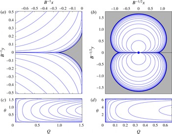
. The streamline pattern of the separable solution is shown in figure 1(a). The key detail of this solution is the appearance of a plug in the vicinity of the origin, which is where the pressure gradient
 $S$
falls below
 $B$
. The yield surfaces bordering this region can be constructed analytically: here, the amplitude is given by (3.7), and so
 $$\begin{eqnarray}\displaystyle p\sim B^{3}a_{2}\cos 2{\it\theta}, & & \displaystyle\end{eqnarray}$$
implying that the corresponding limiting streamline from (3.5) is given by
 $$\begin{eqnarray}\displaystyle (x,y)={\textstyle \frac{1}{3}}B^{2}a_{2}(\cos 3{\it\theta}+3\cos {\it\theta},\sin 3{\it\theta}-3\sin {\it\theta}). & & \displaystyle\end{eqnarray}$$
Thus, for
 ${\it\theta}\rightarrow 0$
,
 $(x,y)\rightarrow (4B^{2}a_{2}/3,0)\approx (-0.2415B,0)$
, which gives the upstream length of the plug (which is also the plug half-length along the wall at
 $x=0$
).
Streamlines for the separable solutions with (a,c)
 $m=2$
and (b,d)
 $m=1/2$
. The plug regions are shaded; (c,d) show the streamlines on the hodograph plane.

A second relevant solution is given by
 $m=1/2$
. In this case, we adopt the limiting solution
 ${\it\psi}\sim -\sqrt{Q}\sin {\it\theta}/2$
for
 $Q\gg 1$
, which corresponds to Newtonian flow around a disk moving through a quiescent ambient with
 $p=-\sqrt{Q}\cos {\it\theta}/2$
,
 $(x,y)=Q^{-1/2}(\cos {\it\theta}/2,\sin {\it\theta}/2)$
and
 ${\it\psi}=-y/(x^{2}+y^{2})$
(in the right half-plane; the flow is symmetric about the
 $y$
axis). The numerical solution of (3.6) then gives
 $a_{1/2}\approx 0.629B^{-5/2}$
, and sample streamlines are shown in figure 1(b). The yield surface, which is again given by the limit
 $Q\rightarrow 0$
, is
 $$\begin{eqnarray}\displaystyle (x,y)={\textstyle \frac{2}{3}}B^{2}a_{1/2}\!\left(\cos {\textstyle \frac{3}{2}}{\it\theta}-3\cos {\textstyle \frac{1}{2}}{\it\theta},\sin {\textstyle \frac{3}{2}}{\it\theta}-3\sin {\textstyle \frac{1}{2}}{\it\theta}\right)\!. & & \displaystyle\end{eqnarray}$$
In order to satisfy the boundary condition on the surface of the disk,
 $x^{2}+y^{2}=1$
, the yield surface must be relatively far away, so that the solution reduces to the Newtonian limit at the disk. Thus, this solution corresponds to viscoplastic flow with a weak yield stress (
 $B\ll 1$
) around a moving disk, and, from (3.10), the yield surface is at a distance of
 $O(B^{-1/2})$
.
4. Circular and elliptical blockages in a uniform cell
We begin our numerical study with a discussion of flow around full obstacles in the cell. At the boundary of the obstacle we impose no normal flux. However, the tangential flow along the boundary cannot be made to vanish due to the Hele-Shaw approximation.
4.1. Flow around a disk
Flow around a disk in a slot with half-width
 $h=1$
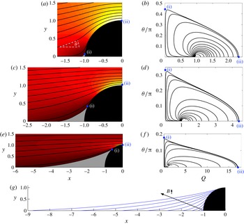
. (a–f) Streamlines with a colour map of
 $Q$
in the
 $(x,y)$
plane (a,c,e), and streamlines in the hodograph plane (b,d,f), for (a,b)
 $B=0.64$
, (c,d)
 $B=20$
, (e,f)
 $B=3200$
. The disk is shaded black and the plugs are shown in grey. The different ranges for the horizontal axes should be noted. Points marked (i) in each plot correspond to
 $(Q,{\it\theta})=(0,{\it\theta}_{\ast })$
, where the plug intersects the disk, and those marked (ii) correspond to
 $(x,y)=(0,1)$
, where the flux is maximum and the flow horizontal. (g) Yield surfaces for several values of
 $B$
separated by a factor of
 $4$
between
 $B=0.2$
and
 $B=5.1\times 10^{4}$
.

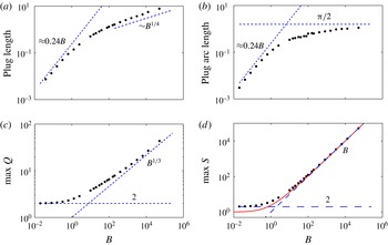
Flow around a disk. (a) The upstream length of the plug ahead of the front of the disk, (b) the arclength along the disk from
 $y=0$
to the edge of the plug, (c) the maximum flux and (d) the maximum pressure gradient, all plotted against
 $B$
. The dashed lines show the theoretical predictions for
 $B\ll 1$
(see § 3.2) and
 $B\gg 1$
(see appendix B). The red solid line in (d) shows the pressure gradient in the far field
 $S_{\infty }(B)\equiv S(1;B,1)$
.

Numerical solutions for flow around a circular blockage are shown for different values of the yield stress
 $B$
in figure 2. The flow is symmetrical about both coordinate axes, and so solutions are shown over only one quadrant. With a finite yield stress, plugs appear at the front and back of the obstacle (denoted by the shaded regions in the figure) spanning a fraction of the disk surface. As
 $B$
is increased, these plugs lengthen in the flow direction, to become much longer than the diameter of the obstacle, and widen such that an increasingly large fraction of the disk lies within the yield surface (figure 2
g).
Figure 2(b,d,f) displays streamlines on the hodograph plane; the yield surface is given by a section of the
 $Q=0$
axis between
 ${\it\theta}=0$
(where the incoming or outgoing streamline along the
 $x$
axis intersects the tip of the plugs) and
 ${\it\theta}={\it\theta}_{\ast }$
, corresponding to the border of the plug on the disk. The streamline leaving
 $(Q,{\it\theta})=(0,{\it\theta}_{\ast })$
represents the fluid path along the yielded surface of the disk and delineates the periphery of the flow region on the hodograph plane in
 $Q>0$
. The point where this bounding streamline intersects the
 $Q$
axis corresponds to the edge of the disk at its widest point
 $(x,y)=(0,\pm 1)$
, and is where the flux is largest. Somewhat surprisingly, as the yield stress is increased the maximum flux increases, which indicates that fluid with a larger yield stress travels more rapidly, at least locally. In the physical plane, the flux is enhanced in increasingly narrow high-speed boundary layers that arise around the widest section of the disk, as can be observed in the colour plots of
 $Q$
(e.g. figure 2
e).
Figure 3 shows a collection of numerical results over a range of values of
 $B$
. For
 $B\ll 1$
, the plugs shrink to narrow regions surrounding the fore and aft points of the disk, and the obstacle appears locally to be a plane wall. The length of the plug in the flow direction converges to
 $0.24B$
in this limit (figure 3
a), which is the result for the separable stagnation-point-flow solution calculated in § 3.2 and shown in figure 1. The arclength of the plug along one quarter of the disk converges to the same value (figure 3
b), as expected from the symmetry of the stagnation-point flow. The flow away from the plugs reduces to the Newtonian result
 ${\it\psi}=y/(x^{2}+y^{2})-y$
for
 $B\ll 1$
, as illustrated by the limiting values of the maximum flux and pressure gradient (figure 3
c,d), which both equal
 $2$
and occur at the widest points of the disk.
For
 $B\gg 1$
, the length of the plugs grows like
 $B^{1/4}$
and the arclength on a quarter of the disk approaches
 ${\rm\pi}/2$
(figure 3
a,b). The maximum flux increases like
 $B^{1/3}$
(figure 3
c) and the maximum magnitude of the pressure gradient increases like
 $B$
(figure 3
d), as it must in order to achieve any flow through the cell as a whole. All of these observations are rationalized by the scaling analysis in appendix B, which identifies three characteristic regions of the flow based on an analysis of the hodograph plane: a relatively long inflow or outflow away from the disk, a narrow high-speed boundary layer around the widest part of the obstacle, and the flow in the vicinity of the yield surface.
4.2. Flow around an ellipse
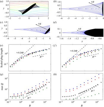
Computations of the flow past elliptical blockages are summarized in figure 4. We scale the semimajor axis of the ellipse to unity; the figure shows results for different eccentricities
 $e$
and inclination angles
 ${\it\alpha}$
of the semimajor axis with respect to the incoming flow. The qualitative features of the flow patterns for different values of
 $B$
are similar to the case of a circular obstacle. When
 $B>0$
, plugs appear at the front and back of the obstacle, and, in the limit
 $B\rightarrow 0$
, they again shrink to small wedges centred on the Newtonian stagnation points with a shape given by the separable solution in figure 1. As
 $B$
is increased, the plug regions again become much longer than the cross-sectional width of the obstacle and span much of the surface of the ellipse (figure 4
b–d). For a tilted ellipse, the plugs bend around as they lengthen to align with the direction of the incident flow (figure 4
c). Thus, for
 $B\gg 1$
, the detailed shape of the obstacle is largely hidden within the shadow of the plug region, and one expects the eccentricity and orientation of the ellipse to matter only in how they dictate the cross-sectional width of the obstruction. Indeed, if one rescales lengths so as to set to unity the cross-sectional width perpendicular to the incident flow (figure 4
e,f), the plug extent converges towards the same scaling for
 $B\gg 1$
, irrespective of
 $e$
and
 ${\it\alpha}$
.
Flow around elliptical obstacles in a slot with half-width
 $h=1$
. (a) Streamlines for flow past an ellipse with
 $e=0.99$
incident at an angle of
 ${\it\alpha}={\rm\pi}/4$
, for
 $B=20.48$
. (b–d) Yield surfaces for values of
 $B$
between
 $B=0.02$
and
 $B=2.1\times 10^{4}$
for an elliptical obstacle with
 $e=0.99$
, inclined at three different angles (
 ${\it\alpha}={\rm\pi}/2$
(b),
 ${\rm\pi}/4$
(c), 0 (d)) to the incoming flow. (e–h) Measurements of the upstream length of the plug region scaled by the cross-sectional width of the obstacle perpendicular to the flow direction, and the maximum flux, for ellipses with eccentricity (e,g)
 $e=0.9$
and (f,h)
 $e=0.99$
, and incident angle
 ${\it\alpha}=0$
(green),
 ${\it\alpha}={\rm\pi}/4$
(red) and
 ${\it\alpha}={\rm\pi}/2$
(blue). The stars show results for a circular disk (figure 3) and the dashed lines indicate asymptotic scalings (see § 3.2 and appendix B).

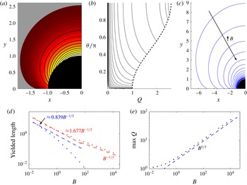
Flow around a disk moving in the positive
 $x$
direction through a uniform slot (
 $h=1$
). (a) Streamlines with a colour map of
 $Q$
in the
 $(x,y)$
plane for
 $B=1.28$
and (b) corresponding streamlines in the hodograph plane; the dashed line indicates the edge of the disk. The disk is shaded black and the plug region is shown in grey. (c) Yield surfaces for varying
 $B$
between
 $B=0.02$
and
 $B=1\times 10^{4}$
. (d) The length of the yielded region along the upstream (
 $y=0$
; blue) and cross-stream (
 $x=0$
; red) axes, together with the limiting values for
 $B\ll 1$
(see § 3.2), and (e) the maximum flux. The asymptotic scalings for
 $B\gg 1$
are also shown dashed in (d) and (e).

As for the circular obstruction, the maximum flux limits to the Newtonian values for
 $B\rightarrow 0$
and scales as
 $Q\sim B^{1/3}$
for large
 $B$
in narrow high-speed boundary layers at the extremities of the obstacle. Because these boundary layers must align with the local geometry, an imprint of the shape of the obstacle remains in the measured maximum flux, which prevents any collapse in figure 4(g,h) for
 $B\gg 1$
. For a given eccentricity, the maximum flux increases with orientation from head-on flow (
 ${\it\alpha}=0$
) to broadside-on (
 ${\it\alpha}={\rm\pi}/2$
) flow.
4.3. A moving disk
The solution for flow around a disk moving through a quiescent Newtonian fluid in a Hele-Shaw cell is simply a translation of the flow past a stationary disk, with the feature that
 $Q=1$
on the surface of the disk. This result no longer applies for a viscoplastic fluid, due to the nonlinearity of the problem. In particular, unyielded plugs arise sufficiently far from the object due to the waning stresses exerted on the fluid, leading to localized flow around the object; see figure 5(a). In the
 $(Q,{\it\theta})$
hodograph plane, the boundary corresponding to the surface of the disk,
 $x^{2}+y^{2}=1$
, deforms away from
 $Q=1$
for
 $0\leqslant {\it\theta}\leqslant {\rm\pi}/2$
into a non-trivial curve bounding the flow region (figure 5
b).
The shape of the yield surface in these solutions (figure 5
c) shows some qualitative similarities with the corresponding surfaces for two-dimensional flow of viscoplastic fluid around cylinders or axisymmetric flow around spheres (Beris et al.
Reference Beris, Tsamopoulos, Armstrong and Brown1985), although, unlike in those situations, here there are no plugs attached to the disk itself. For
 $B\ll 1$
, the yielded region is relatively large, scaling as
 $B^{-1/2}$
in both spatial directions (figure 5
d), in accord with the separable hodograph solution shown in figure 1(b). For
 $B\gg 1$
, the yielded zone shrinks to become a narrow boundary layer shrouding the disk, with a width that scales like
 $B^{-1/3}$
(figure 5
d). This scaling demands that the maximum flux reaches values of order
 $B^{1/3}$
(figure 5
e), in order to maintain the imposed
 $O(1)$
flux. Both scalings can again be rationalized by a scaling analysis of equations in the hodograph domain, similar to that undertaken in appendix B.
5. Cell contractions and expansions
A sudden contraction or expansion in the width provides a different kind of obstacle to flow along a Hele-Shaw cell, by impeding or diverting viscous flow but not directly blocking it. In the context of flow through a porous medium, a change in width is equivalent to a change in the permeability of the medium, and step changes in permeability over a disk or lens provide a classical model of flow around and through various geological formations (e.g. Phillips Reference Phillips2009).
In this section, we focus predominantly on viscoplastic flow through circular contractions and expansions. We set
 $h=1$
outside and
 $h={\it\xi}$
inside the obstacle, such that
 ${\it\xi}$
dictates the contraction or expansion ratio. At the border of the obstacle, we smooth out the jump in slot thickness over a narrow layer of the order of tens of gridpoints, such that the border remains relatively sharp, but the coefficients in (2.19) remain smooth and no special jump conditions are required when numerically computing the solution for
 ${\it\psi}$
. This procedure is equivalent to enforcing the continuity of normal flux in the limit of a genuine step change in
 $h(x,y)$
. For comparison, we note that the corresponding streamfunction for Newtonian flow impinging on a circular contraction or expansion can be determined analytically and is
 $$\begin{eqnarray}\displaystyle {\it\psi}=\frac{(1-{\it\xi}^{3})y}{(1+{\it\xi}^{3})(x^{2}+y^{2})}-y\quad \text{if }x^{2}+y^{2}<1, & & \displaystyle\end{eqnarray}$$
while within the obstacle the solution has uniform flux in the
 $x$
direction:
 ${\it\psi}=2{\it\xi}^{3}y/({\it\xi}^{3}+1)$
.
5.1. Contractions
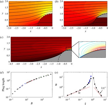
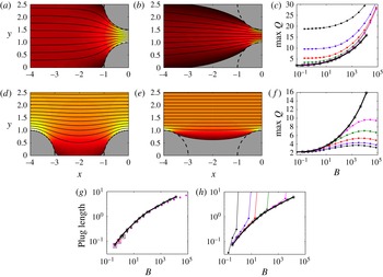
Figure 6(a–c) displays solutions for viscoplastic flow incident on a circular cell contraction with a dimensionless width of
 $2{\it\xi}=1$
(the contraction is half as wide as the surrounding slot). When the fluid has a relatively low yield stress (figure 6
a), the flow remains yielded everywhere. Within the contraction, the fluid has an almost uniform flux, reflecting the remnant of this feature of the Newtonian solution. When the fluid has a slightly higher yield stress (figure 6
b), the contraction begins to plug up, with stagnant zones appearing at its peripheries. For larger values of
 $B$
, the contraction becomes fully plugged (figure 6
c). In this situation, the blockage prompts the formation of wedge-shaped plugs outside the contraction and the flow pattern is very similar to the corresponding solution for a full circular obstacle, as illustrated by the upstream length of the plug (figure 6
d). There is, however, a subtle difference in the boundary conditions in the high-speed boundary layers above and below the obstacle. A full barrier across the cell prevents any normal flow but allows tangential slip within the Hele-Shaw approximation. By contrast, a plugged contraction is bordered by a yield surface along which
 $Q=0$
, which corresponds to a no-slip boundary. This feature is illustrated in the inset of figure 6(c), which shows how the flux decreases to zero at the edge of the plugged contraction. The flux gradient arises over the layer where the change in slot thickness is smoothed in the numerical computations, and reduces the maximum flux in comparison to that for a full obstacle, for which the flux peaks at the edge of the disk.
(a–c) Streamlines and colour maps of
 $Q$
for flow past a circular contraction of width
 $2{\it\xi}=1$
, for (a)
 $B=0.8$
, (b)
 $B=6.4$
and (c)
 $B=205$
. The plugs are shaded. The inset in (c) shows the contours of
 $Q$
in the thin boundary layer that arises at the widest points of the disk, where, unlike in the case of a full obstacle, the flux decreases to zero at the edge of the plugged contraction. (d) Upstream length of the plug ahead of the disk for
 ${\it\xi}=0.1$
(black),
 ${\it\xi}=0.25$
(blue),
 ${\it\xi}=0.5$
(red) and
 ${\it\xi}=0.75$
(green). The stars show corresponding results for a full obstruction (i.e.
 ${\it\xi}=0$
, from figure 3). (e) The critical Bingham number above which a plug first appears (black) or the disk becomes fully plugged up (blue), including results for expansions (
 ${\it\xi}>1$
) as well as contractions
 $({\it\xi}<1)$
. The red lines denote asymptotic predictions for
 ${\it\xi}\ll 1$
and
 ${\it\xi}\gg 1$
, as marked.

The critical Bingham number for which a plug first appears is plotted as a function of the degree of contraction
 ${\it\xi}$
in figure 6(e), along with the value of
 $B$
above which the contraction is completely plugged. The window of yield stresses over which the obstacle is partially plugged is relatively small. For
 ${\it\xi}=1$
, there is no obstacle and hence no plugs form. Conversely, for
 ${\it\xi}\rightarrow 0$
, an arbitrarily small yield stress will plug up the contraction, in line with the result that plugs are always present for a complete obstruction when
 $B>0$
. For
 ${\it\xi}\rightarrow 0$
, the limiting critical Bingham number for the obstacle to plug up can be predicted by observing that the Newtonian solution (5.1) has a constant pressure gradient of
 $S=2/(1+{\it\xi}^{3})$
within the contraction, whereas the yield condition is
 $Y=B/S={\it\xi}$
. Hence,
 $B\rightarrow 2{\it\xi}$
if
 ${\it\xi}\rightarrow 0$
, as seen in figure 6(e).
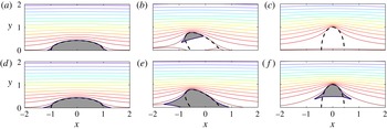
It should be noted that the features of the solutions in figure 6 are not specific to a circular contraction: solutions for an elliptical contraction are plotted in figure 7, which shows how the orientation of the ellipse affects the critical yield stress at which the contraction begins to plug up. Once the contraction is fully blocked, the solutions are much like their counterparts for a complete blockage. Thus, for
 $B\gg 1$
, both blockages and contractions arrest motion along an increasingly long strip whose thickness is dictated by the width of the obstacle perpendicular to the flow. In other words, at the onset of motion (the limit
 $B\rightarrow \infty$
) the obstacle blocks off an entire strip of the whole cell.
Streamlines for flow past an elliptical contraction of width
 $2{\it\xi}=1$
(dashed), for
 $B=12.8$
(a–c) and
 $B=51.2$
(d–f). The ellipse has eccentricity
 $e=0.9$
, and is aligned at an angle (a,d)
 ${\it\alpha}=0$
, (b,e)
 ${\it\alpha}={\rm\pi}/4$
, and (c,f)
 ${\it\alpha}={\rm\pi}/2$
to the incoming flow. The plugs are shaded.

5.2. Expansions
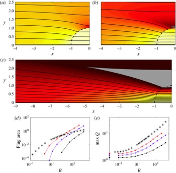
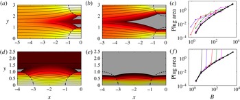
Results for flow past circular expansions are shown in figure 8. For sufficiently low values of
 $B$
(figure 8
a), there are no plugs and the flow resembles the Newtonian solution; fluid is diverted through the expansion, and the flow is slowest just above and below the expansion. For larger
 $B$
(figure 8
b), plugs appear in these low-speed regions. As
 $B$
is increased further, the plugs extend significantly upstream and downstream and invade the expansion (figure 8
c). For large values of
 $B$
, the plugs divert far more fluid through the expansion than for
 $B=0$
, and establish a surprisingly far-field influence of the obstacle relative to the Newtonian problem.
Figure 8(d) shows that the area of the plug increases with both the expansion ratio
 ${\it\xi}$
and
 $B$
, and, rather counterintuitively, indicates that expansions lead to a larger plugged region than contractions and full blockages for sufficiently large values of
 $B$
. The maximum flux increases with
 ${\it\xi}$
and
 $B$
(figure 8
e), and, for
 $B\gg 1$
, appears to show the same scaling as for flow past a full blockage, although it now occurs through the centre of the expansion. In the limit
 $B\rightarrow \infty$
, the area of the buffering plugs diverges, which indicates that, at the onset of motion, the expansion funnels all of the flow through its core, and leaves plugged wedges of fluid extending from either side.
(a–c) Streamlines and colour maps of flow past a circular expansion with width
 $2{\it\xi}=3$
, for (a)
 $B=0.8$
, (b)
 $B=36.2$
and (c)
 $B=4634$
. Plug regions are shaded. (d) Plug area and (e) maximum flux, plotted against
 $B$
, for
 ${\it\xi}=1.2$
(black),
 ${\it\xi}=1.5$
(blue) and
 ${\it\xi}=2$
(red). The stars show corresponding results for a full obstruction (i.e.
 ${\it\xi}=0$
; from figure 3). The points at
 $B=0$
indicate the Newtonian solution.

The critical values of
 $B$
at which the plugs first appear are shown in figure 6(e). For
 ${\it\xi}\rightarrow \infty$
, plugs are present for all
 $B>0$
, because the Newtonian solution (5.1) features stagnation points at
 $(x,y)=(0,\pm 1)$
in this limit. In fact, locally, the top and bottom of the expansion appear to be plane boundaries with purely normal flow, and a matched asymptotic expansion for
 $B\ll 1$
can be used to show that the local viscoplastic flow is given by the stagnation-point solution of § 3.2, but rotated by
 $45^{\circ }$
. We can predict the critical value of
 $B$
at which the plug appears in this limit by noting that the Newtonian pressure gradient
 $S$
outside the disk approaches
 $2/{\it\xi}^{3}$
at
 $(x,y)=(0,\pm 1)$
. Hence,
 $Y=B/S\rightarrow 1$
when
 $B\rightarrow 2/{\it\xi}^{2}$
, as shown in figure 6(e).
6. More complicated geometries
6.1. Arrays of obstacles
A natural extension of the results for isolated obstacles in §§ 4 and 5 is to consider arrays of such obstacles, and examine whether multiple objects interfere constructively or destructively in the flow patterns. Accordingly, in this section we present results for periodic arrays of circular contractions and expansions, separated vertically or horizontally by a distance
 ${\it\Lambda}$
. We focus on linear arrays orientated either with the flow direction or perpendicular to it, and then briefly discuss two-dimensional arrays in a square or staggered arrangement.
Flow past periodic arrays of circular contractions with
 ${\it\xi}=0.1$
. (a,b) Streamlines and a colour map of
 $Q$
for contractions arranged perpendicular to the flow with
 ${\it\Lambda}=1/2$
and (d,e) aligned with the flow with
 ${\it\Lambda}=2$
, for (a,d)
 $B=1.6$
and (b,e)
 $B=409.6$
. Plug regions are shaded. (c,f) Maximum flux, and (g,h) length of the plug upstream of the obstacle for perpendicular arrays (c,g)
 ${\it\Lambda}=1/8$
(black),
 ${\it\Lambda}=1/4$
(blue),
 ${\it\Lambda}=1/2$
(red),
 ${\it\Lambda}=1$
(green) and
 ${\it\Lambda}=2$
(pink); and for aligned arrays (f,h)
 ${\it\Lambda}=1$
(black),
 ${\it\Lambda}=2$
(blue),
 ${\it\Lambda}=4$
(red),
 ${\it\Lambda}=8$
(green) and
 ${\it\Lambda}=16$
(pink). Results for an isolated contraction are shown by black stars and a solid line. In (g), the squares indicate the lowest value of
 $B$
for which a plug exists. In (h), when the downstream plug of one obstacle intersects the upstream plug of the next obstacle, the length of the plug diverges.

We first consider periodic arrays of contractions (figure 9). When arranged perpendicular to the flow (figure 9
a,b), the contractions channel the flow into the gaps between them, raising the maximum flux (figure 9
c) and delaying the plugging up of those obstacles (figure 9
g), effects that are enhanced if
 ${\it\Lambda}$
is reduced. However, once contractions have been blocked and the plugs extend upstream and downstream, the size of the plug for each member of the array (figure 9
g) is little different than if the contraction were isolated. Thus, arranging the contractions perpendicular to the flow has a relatively minor effect on the flow patterns.
Flow past infinite arrays of circular expansions with
 ${\it\xi}=2$
. (a,b) Streamlines and a colour map of
 $Q$
for expansions arranged perpendicular to the flow with
 ${\it\Lambda}=1$
and (d,e) aligned with the flow with
 ${\it\Lambda}=2$
, for (a,d)
 $B=18.1$
and (b,e)
 $B=409.6$
. Plug regions are shaded. (c,f) Area of the plug regions, for perpendicular arrays (c)
 ${\it\Lambda}=1/4$
(blue),
 ${\it\Lambda}=1/2$
(red),
 ${\it\Lambda}=1$
(green) and
 ${\it\Lambda}=2$
(pink); and for aligned arrays (f)
 ${\it\Lambda}=1$
(black),
 ${\it\Lambda}=2$
(blue),
 ${\it\Lambda}=4$
(red),
 ${\it\Lambda}=8$
(green) and
 ${\it\Lambda}=16$
(pink). Results for an isolated expansion are plotted as black stars and a solid line. When the downstream plug of one obstacle reaches the upstream plug of the next obstacle, the area of the plug diverges.

A more significant effect is observed if contractions are aligned in the direction of the flow (figure 9
d,e). In this case, the presence of neighbouring contractions lowers the maximum flux (figure 9
f) and increases the length of the plugs (figure 9
h). More importantly, above a critical value of
 $B$
, which decreases with the separation distance
 ${\it\Lambda}$
, the plugs of neighbouring contractions merge, at which point the effective plug length diverges with an uninterrupted stagnant zone bridging the gaps between the contractions.
We next address periodic arrays of expansions (figure 10). When expansions are arranged perpendicular to the flow (figure 10
a,b), the convergence of flow into the expansions weakens the flow between them, which results in plugs that are larger and form at lower yield stresses than for an isolated expansion (figure 10
c). For larger values of
 $B$
, neighbouring pairs of plugs merge together (figure 10
b), but the presence of the expansions impedes the combined plugs from growing too large.
As for contractions, a more significant effect is observed if expansions are aligned with the direction of the flow (figure 10
d,e). Above a critical value of
 $B$
, which increases with the separation distance
 ${\it\Lambda}$
, the plugs merge to form an uninterrupted stagnant layer (figure 10
f) and flow becomes channelized through the expansions. Even below this threshold, although the plug area is similar to that for an isolated expansion, there is a significant reduction in the flow through the part of the slot that is not aligned with the expansion (e.g. dark shaded area in figure 10
d).
Thus, for linear arrays, periodic contractions or expansions interfere most effectively when aligned with the flow direction (i.e. in series), rather than when arrayed perpendicular to the flow (i.e. in parallel). In terms of plug area, the interference of periodic arrays is constructive, and stronger for expansions than contractions. In the limit
 $B\rightarrow \infty$
, or equivalently at the onset of motion, arrays aligned periodically in the flow direction channelize the flow through the gaps between contractions or within the expansions themselves.
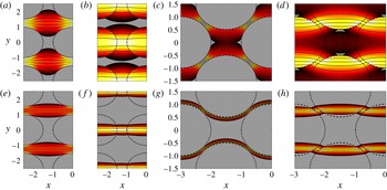
Many of these results carry over to fully two-dimensional arrays of obstacles: as illustrated in figure 11, on raising
 $B$
, plugs fill the contractions, appear around the regions where the flow is slowest in the Newtonian solutions, and then expand to merge horizontally, thereby channelizing the flow. For yet larger
 $B$
, the channels become thinner and wend their way around the topography, in such a manner as to preferentially sample the widest parts of the slot. This channelization allows the flow either to avoid contractions, rendering the net resistance dependent only on the tortuosity of the path taken, or to pass through expansions, which lowers the resistance to flow.
Solutions for flow past arrays of circular obstacles at
 $B=3.2$
(a–d) and
 $B=820$
(e–h). Streamlines and colour maps of
 $Q$
for sample (a,b,e,f) square and (c,d,g,h) staggered arrays; (a,c,e,g) show solutions for contractions with
 ${\it\xi}=0.2$
; (b,d,f,h) show solutions for expansions with
 ${\it\xi}=2$
.

6.2. Randomly roughened cells
A significantly more complex geometry is provided by a cell with randomly roughened walls. To generate a ‘rough’ conduit, we consider a periodic domain of unit length in the
 $x$
direction and take the half-thickness
 $h$
to be a suitable random function of spatial position. More specifically, we introduce a roughness function
 $F$
given by a random Fourier series in both directions, each truncated at a wavenumber
 $k_{t}$
, and set
 $$\begin{eqnarray}\displaystyle \hspace{-20.00003pt}h=1+{\it\sigma}F,\quad F(x,y)=\text{Re}\,\left\{\mathop{\sum }_{m=-k_{t}}^{k_{t}}\mathop{\sum }_{n=-k_{t}}^{k_{t}}\frac{a_{mn}\exp [2{\rm\pi}\text{i}(mx+ny)]}{\max [1,(m/k_{\ast })^{{\it\alpha}}]\max [1,(n/k_{\ast })^{{\it\alpha}}]}\right\}, & & \displaystyle\end{eqnarray}$$
where the complex coefficients
 $a_{mn}$
are randomly selected from a uniform distribution on
 $[-A,A]$
, with
 $A$
chosen such that
 $F^{2}$
has a spatial average of unity. The parameter
 ${\it\sigma}$
controls the amplitude of the roughness around the average cell half-width of
 $1$
. The parameters
 $k_{\ast }$
and
 ${\it\alpha}$
control the smoothing of the roughness, such that the Fourier coefficients decay with a power of
 ${\it\alpha}$
for wavenumbers greater than
 $k_{\ast }$
. It should be noted that the assumptions in § 2 of a thin slot remain valid provided that the slope of the roughness is small relative to the aspect ratio of the cell, such that
 ${\it\sigma}k_{\ast }\ll L/H$
.
Density maps of flux
 $Q$
from one realization of flow along a cell with randomly roughened walls (
 ${\it\alpha}=2$
,
 $k_{t}=30$
and smoothing scale
 $k_{\ast }=10$
). Different Bingham numbers of (a,d,g)
 $B=0.01$
, (b,e,h)
 $B=100$
and (c,f,i)
 $B=10^{5}$
are plotted, and the roughness has standard deviation (a,b,c)
 ${\it\sigma}=0.05$
, (d,e,f)
 ${\it\sigma}=0.1$
and (g,h,i)
 ${\it\sigma}=0.3$
. The inset in (a) shows a greyscale density plot of the roughness
 $F(x,y)$
of the channel over the range
 $0\leqslant x\leqslant 0.5$
,
 $0.5\leqslant y\leqslant 1$
.

Figure 12 shows density maps of the flux for one realization of the slot with
 ${\it\alpha}=2$
,
 $k_{t}=30$
and
 $k_{\ast }=10$
, for three choices of both
 ${\it\sigma}$
and
 $B$
. When the yield stress is very low (a,d,g), the solutions are little different than if the flow were Newtonian: the roughness triggers the development of structure in the flow patterns with a scale comparable to the smoothing length
 $k_{\ast }^{-1}$
. When the amplitude of the roughness is sufficiently large (g–i), the slot almost closes off in several locations and incipient channels can be discerned in the flow field.
More dramatically, when the yield stress is increased, the flow fully channelizes into localized conduits. These channels are present even for smaller levels of roughness (i.e.
 ${\it\sigma}=0.05$
; a–c) provided that the yield stress is sufficiently high, and follow paths with little deviation from the flow direction. For cells with a larger amplitude of roughness, the channels migrate further from the flow direction, but in none of the cases is there an obvious correlation with distinctive features of the ‘topography’ in
 $h(x,y)$
(shown in part of figure 12
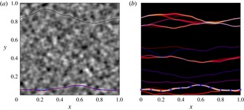
a, and again in more detail in figure 14 below). We attribute the channelization to the accidental alignment of either contractions or expansions in the flow direction; that is, plugged lines of contractions and high-speed conduits through aligned expansions conspire to create the channel network. However, the lack of any obvious correlation between the geometries of the network and topography indicates that the conspiracy is relatively subtle, and the factors that dictate the locations of the channels demand more analysis. It should be noted that similar channelization to that shown in figure 12 has previously been observed in lattice Boltzmann simulations of two-dimensional flow of Bingham fluids through complex networks (Talon & Bauer Reference Talon and Bauer2013).
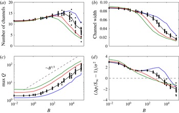
Averages over
 $20$
different realizations of the roughness with the same parameter settings as figure 12, showing (a) the average number of channels, (b) the average width of the channels, (c) the maximum flux
 $Q$
and (d) the relative deviation of the average pressure drop across the cell,
 ${\rm\Delta}p$
, from the value for a uniform cell,
 $S_{\infty }$
, scaled by
 ${\it\sigma}^{2}$
. The method of calculation of
 ${\rm\Delta}p$
is described in appendix C. Negative values indicate that the effective permeability (
 $1/{\rm\Delta}p$
) is increased relative to a uniform cell. Data are shown for
 ${\it\sigma}=0.05$
(blue),
 ${\it\sigma}=0.1$
(black),
 ${\it\sigma}=0.2$
(red) and
 ${\it\sigma}=0.3$
(green). Dots show individual realizations for
 ${\it\sigma}=0.1$
.

Optimal paths for the realization of the topography from figure 12. (a) Density map of the topography overlain by the break-through channels for
 ${\it\sigma}=0.05$
(solid),
 ${\it\sigma}=0.1$
(dashed) and
 ${\it\sigma}=0.3$
(short dashed). (b) A density map of
 $Q$
from the numerical flow solution for
 ${\it\sigma}=0.1$
and
 $B=10^{5}$
, as in figure 12(f), overlain by a selection of optimal paths (thin blue lines). The stars indicate the break-through channel.

Further details of solutions for multiple realizations are presented in figure 13. To define ‘channels’ in these solutions we identify distinct regions in the
 $y$
direction at each streamwise position
 $x$
for which
 $Q>1$
. The average number and width of such regions over
 $x$
provide the mean channel number and width. Once plugs appear, the number of channels and their width decrease as
 $B$
is increased (figure 13
a–b), leading to large areas of stagnant or near-stagnant flow for high yield stress (cf. figure 12
c,f,i). Simultaneously, the flow through the channels becomes faster, with the maximum fluxes scaling with
 $B^{1/3}$
(figure 13
c). Figure 13(d) shows a scaled average pressure drop across the cell. The definition of a mean pressure drop is complicated by the presence of stagnant plugs in the flow, inside which the pressure is formally undefined. We determine the pressure drop by a suitable integration along streamlines, thereby avoiding plugged regions, as described in appendix C.
Given the scaling of the problem, the inverse of the pressure drop
 $1/{\rm\Delta}p$
defines an effective permeability. In a uniform cell,
 ${\rm\Delta}p=S_{\infty }(B)$
, which increases with
 $B$
, reflecting how the rheology of the fluid controls the pressure force required to achieve flow. Even when one roughens the walls of the cell, this rheological effect dominates the pressure drop, such that
 ${\rm\Delta}p\propto S_{\infty }$
for large
 $B$
. In figure 13(d), we therefore use the scaled relative pressure drop
 $({\rm\Delta}p-S_{\infty })/S_{\infty }$
to remove the dominant rheological effect. For low
 $B$
, the relative pressure drop is positive, indicating that the effective permeability of the roughened cell is lower than that of the uniform cell. However, for higher
 $B$
when the flow has channelized,
 $({\rm\Delta}p-S_{\infty })/S_{\infty }<0$
. Thus, a channelized rough conduit is more permeable than a uniform cell.
To collapse the results for different scales of roughness, we further scale the relative pressure drop by
 ${\it\sigma}^{2}$
, which corresponds to the dependence expected for a Newtonian fluid in a cell with low-amplitude roughness (Zimmerman & Bodvarsson Reference Zimmerman and Bodvarsson1996). The scaling with
 ${\it\sigma}^{2}$
arises because the flow encounters variations in the width with zero spatial average, which demands that resistance is modified at second order. On the other hand, for larger values of
 $B$
, the fluid is diverted into channels that are, on average, wider than the mean cell width, leading to a deviation from the scaling of the relative pressure drop with
 ${\it\sigma}^{2}$
(figure 13
d).
The results of this section suggest that, in the limit
 $B\rightarrow \infty$
, a network of a small number of infinitely narrow channels survives. As discussed in § 2.3, this limit corresponds to the flow at the initiation of motion. In fact, when the slot has no spatial symmetry (other than the base periodicity), multiple channels are unlikely to support equal pressure drops, and so it is natural to anticipate that channels continue to disappear, with all but one vanishing in the asymptotic limit
 $B\rightarrow \infty$
(as in figure 12
i). In the following section, we show that this ‘break-through’ channel can be constructed more directly using an optimization procedure.
6.3. Break-through channels
6.3.1. The optimization problem
The infinitely narrow channel that opens up in the limit
 $B\rightarrow \infty$
is characterized by
 $Y\rightarrow h$
all the way along its length, or
 $S\sim B/h(x,y)$
. At first sight (since
 $S^{2}\equiv p_{x}^{2}+p_{y}^{2}$
), this suggests that the pressure satisfies the eikonal equation. However, the limiting channel constitutes a curve on the
 $(x,y)$
plane, and
 $S\sim B/H$
applies only along its course. Thus, if the curve is parameterized by its arclength
 $s$
, we have
 $$\begin{eqnarray}\displaystyle \frac{\,\text{d}p}{\,\text{d}s}=\frac{B}{h(x(s),y(s))},\quad \left(\frac{\,\text{d}x}{\,\text{d}s}\right)^{2}+\left(\frac{\,\text{d}y}{\,\text{d}s}\right)^{2}=1, & & \displaystyle\end{eqnarray}$$
and the scaled pressure drop across this pathway is
 $$\begin{eqnarray}\displaystyle \frac{1}{B}{\rm\Delta}p=\frac{1}{B}[p(x(s),y(s))]_{s=0}^{\ell }=\int _{0}^{\ell }\frac{\,\text{d}s}{h(x(s),y(s))}, & & \displaystyle\end{eqnarray}$$
where
 $\ell$
is the total path length. The path with the lowest pressure drop can therefore be determined by searching for the minimum of the functional
 $$\begin{eqnarray}\displaystyle \int _{0}^{\ell }\left[\frac{1}{h}-{\it\lambda}(s)(1-x_{s}^{2}-y_{s}^{2})\right]\,\text{d}s, & & \displaystyle\end{eqnarray}$$
where
 ${\it\lambda}(s)$
is a Lagrange multiplier.
For our periodic unit cells, the path must have the endpoints
 $[x(0),y(0)]=[0,y_{0}]$
and
 $[x(\ell ),y(\ell )]=[1,y_{0}]$
, for some
 $0\leqslant y_{0}\leqslant 1$
. This condition translates to the imposition of homogeneous boundary conditions when considering the variations of the channel path about the optimal solution. The Euler–Lagrange equations for the optimal path are then
 $$\begin{eqnarray}\displaystyle 2({\it\lambda}x_{s})_{s}+\frac{h_{x}}{h^{2}}=2({\it\lambda}y_{s})_{s}+\frac{h_{y}}{h^{2}}=0, & & \displaystyle\end{eqnarray}$$
along with the constraint
 $x_{s}^{2}+y_{s}^{2}=1$
. Multiplying the first relation in (6.5) by
 ${\it\lambda}x_{s}$
and the second by
 ${\it\lambda}y_{s}$
, then adding the results, leads to
 $({\it\lambda}-h^{-1})_{s}=0$
. Hence, we take
 ${\it\lambda}=h^{-1}$
to obtain
 $$\begin{eqnarray}\displaystyle x_{{\it\xi}{\it\xi}}+\frac{y_{{\it\xi}}}{h}(h_{x}y_{{\it\xi}}-h_{y}x_{{\it\xi}})=y_{{\it\xi}{\it\xi}}+\frac{x_{{\it\xi}}}{h}(h_{y}x_{{\it\xi}}-h_{x}y_{{\it\xi}})=0, & & \displaystyle\end{eqnarray}$$
where
 ${\it\xi}=s/\ell$
. By using the variable
 ${\it\xi}$
, we may avoid the unknown path length
 $\ell$
, and the boundary conditions become
 $[x(0),y(0)]=[0,y_{0}]$
and
 $[x(1),y(1)]=[1,y_{0}]$
. Although in general it is straightforward to construct numerical solutions to (6.6) for an arbitrary starting position
 $y_{0}$
, these solutions are typically unacceptable because they are not smooth periodic functions in
 $x$
, i.e.
 $x_{s}(0)\neq x_{s}(1)$
and
 $y_{s}(0)\neq y_{s}(1)$
. Only certain special choices of
 $y_{0}$
will lead to acceptable periodic solutions. The set of possible solutions, characterized by these special values of
 $y_{0}$
, correspond to local extrema of the pressure drop (6.2a
), and we identify the solution with the lowest pressure drop as the break-through channel. It should be noted that one can formulate the optimal-path problem using the alternative parameterization
 $y=f(x)$
, which leads to a lower-order system of Euler–Lagrange equations. We use (6.6), however, to avoid any issues with the parameterization becoming multivalued.
The optimization problem that underlies (6.6) amounts to finding the path across the periodic domain that minimizes
 $[h(x(s),y(s))]^{-1}$
, or equivalently maximizes the sampling of local expansions of the slot. However, in view of the path integral, the optimization simultaneously seeks to minimize the path length. Thus, the optimal solutions are those that minimize the deviations from straight lines in the flow direction while preferentially sampling slot expansions. For example, a long winding path that traverses all of the widest sections of the slot is unlikely to give the lowest pressure drop, unless the variations in the width of the cell are very large.
6.3.2. Optimal paths
We begin with a brief outline of some instructive asymptotic limits of the optimization problem. First, if
 $h=h(x)$
, (6.6) has the solutions
 $x({\it\xi})={\it\xi}$
and
 $y({\it\xi})=y_{0}$
, i.e. straight lines parallel to the flow direction. All values of
 $y_{0}$
are acceptable in this instance, as expected when the slot is uniform in
 $y$
and unplugs everywhere simultaneously at the critical pressure drop
 $B^{-1}{\rm\Delta}p=\int _{0}^{1}[h(x)]^{-1}\,\text{d}x$
. Second, if
 $h=h(y)$
, the optimal paths are again straight lines with
 $x({\it\xi})={\it\xi}$
and
 $y({\it\xi})=y_{0}$
, although the only possible values of
 $y_{0}$
satisfy
 $h_{y}(y_{0})=0$
. Thus, unsurprisingly, the first channel opens along the widest expansion of the slot.
Another informative limit is when the conduit is almost uniform, such that
 $h=1+{\it\sigma}F(x,y)$
with
 ${\it\sigma}\ll 1$
. To find the solution in this limit, we set
 $$\begin{eqnarray}\displaystyle x={\it\xi}+{\it\sigma}^{2}x_{2}({\it\xi})+\cdots \quad \text{and}\quad y=y_{0}+{\it\sigma}y_{1}({\it\xi})+{\it\sigma}^{2}y_{2}({\it\xi})+\cdots \,. & & \displaystyle\end{eqnarray}$$
Substituting these sequences into (6.6) gives, to leading order in
 ${\it\sigma}$
,
 $$\begin{eqnarray}\displaystyle y_{1{\it\xi}{\it\xi}}+F_{y}({\it\xi},y_{0})=0,\quad x_{2{\it\xi}{\it\xi}}+y_{1{\it\xi}}F_{y}({\it\xi},y_{0})=0. & & \displaystyle\end{eqnarray}$$
Thus,
 $$\begin{eqnarray}\displaystyle y_{1}={\it\Phi}({\it\xi},y_{0}),\quad x_{2}=-\int _{0}^{{\it\xi}}{\it\Phi}_{{\it\xi}}^{2}\,\text{d}{\it\xi}, & & \displaystyle\end{eqnarray}$$
if
 $F_{y}({\it\xi},y_{0})={\it\Phi}_{{\it\xi}{\it\xi}}({\it\xi},y_{0})$
. Not all of these solutions are acceptable, however, as higher-order corrections may not be periodic. In particular, we must constrain the starting value
 $y_{0}$
by demanding that
 $$\begin{eqnarray}\displaystyle 0=[\,y_{2{\it\xi}}]_{{\it\xi}=0}^{{\it\xi}=1}=\int _{0}^{1}[F({\it\xi},y_{0}){\it\Phi}_{{\it\xi}{\it\xi}}-F_{x}({\it\xi},y_{0}){\it\Phi}_{{\it\xi}}-F_{yy}({\it\xi},y_{0}){\it\Phi}]\,\text{d}{\it\xi}. & & \displaystyle\end{eqnarray}$$
Solutions of (6.10) pick out specific values of
 $y_{0}$
at which channels are initiated. The channels are nearly straight lines, aligned with the pressure gradient; the minimization of the path length overwhelms the preference for local expansions in this limit.
The break-through channels for the realization of the roughness in figure 12 are shown in figure 14(a), overlain on a map of the topography; a selection of some other optimal channels is shown in figure 14(b). The full set of optimal-path solutions and their dependence on
 ${\it\sigma}$
for this realization are excessively convoluted, due to the complexity of the roughness. A more transparent illustration of typical optimal-path solutions is provided by a simpler realization of (6.1) with
 ${\it\alpha}=4$
,
 $k_{\ast }=3$
and
 $k_{t}=20$
, as shown in figure 15(a). Numerical flow solutions at large Bingham number for three values of the roughness amplitude
 ${\it\sigma}$
are shown in figure 15(b–d). For the largest value of
 ${\it\sigma}$
, only one channel remains at this value of
 $B$
, while for smaller
 ${\it\sigma}$
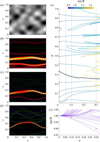
there is still a network of channels. Solutions of (6.6) for the optimal pathways are overlain in these figures, including those corresponding to elevated as well as reduced pressure drops. In each case, the channel with the smallest pressure drop lies along the centre of the dominant channel from the numerical flow solution.
Optimal paths for a realization of the topography (6.1) with
 $k_{\ast }=3$
,
 ${\it\alpha}=4$
and
 $k_{t}=20$
, as shown in (a). (b–d) Density maps of
 $Q$
from full numerical solutions with
 $B=10^{5}$
, overlain by optimal paths, for (b)
 ${\it\sigma}=0.05$
, (c)
 ${\it\sigma}=0.1$
and (d)
 ${\it\sigma}=0.3$
. Stars indicate the path with the lowest pressure drop. Blue (green) indicates
 ${\rm\Delta}p<B$
(
 ${\rm\Delta}p>B$
). (e) An almost complete bifurcation diagram of the optimal paths, coloured according to the scaled pressure drop
 ${\rm\Delta}p/B$
along that path, as a function of the roughness amplitude
 ${\it\sigma}$
. The stars show the path with the lowest pressure drop. The red circles indicate the starting locations for
 ${\it\sigma}\rightarrow 0$
, as given by (6.10). The vertical dashed lines indicate the locations of the three solutions shown in (b–d). (f) The scaled pressure drops of the optimal-path solutions shown in (e), together with the mean values of the full numerical solutions in (b–d) (dots; computed as indicated in appendix C).

In figures 14(b) and 15(b–d), there are a number of solutions that give a favourable pressure drop (i.e.
 ${\rm\Delta}p<\lim _{B\rightarrow \infty }S_{\infty }=B$
) as well as the break-through channel. As illustrated in both of these figures, some of these ‘secondary’ pathways actually pick out other channels in the networks of the flow solutions. In fact, the average pressure drop of the flow solutions in figure 15 is indeed higher than the pressure drops of several secondary channels (figure 15
f), which suggests that they could also open up in addition to the main break-through channel.
Although the optimal paths coincide with favourable topographic features at least somewhere along their lengths, they are very sensitive to the detailed topography, and it is difficult to anticipate from the density plot of
 $h(x,y)$
alone where the break-through channel appears (cf. figure 14
a). Moreover, a small change of parameters can lead to a sudden switch in the location of this pathway, as is evident in figure 14(a), where the break-through channels correspond to two distinct optimal solutions for different values of
 ${\it\sigma}$
. Sometimes, the geometry of a flow channel is also slightly different from any optimal solution, with fluid following one of the paths for part of its course before taking a wrong turn around a topographic feature and then aligning with a second path for the remainder of its journey (examples can be seen in figure 14
b).
An impression of the full richness of the solution structure for the simpler model topography is shown in figure 15(e). This figure shows an almost complete collection of the optimal channel paths, as a bifurcation diagram on the
 $({\it\sigma},y_{0})$
plane. For
 ${\it\sigma}\rightarrow 0$
, there are 15 acceptable values of
 $y_{0}$
, as indicated by circles on the bifurcation diagram. The corresponding pathways are almost straight lines on the physical plane, as illustrated for
 ${\it\sigma}=0.05$
in figure 15(b). Increasing the roughness amplitude
 ${\it\sigma}$
prompts a number of saddle-node bifurcations; two optimal solutions disappear near
 ${\it\sigma}=0.01$
, but many more appear for higher values of
 ${\it\sigma}$
, leading to over 50 solutions at
 ${\it\sigma}=0.33$
. For such high levels of roughness, there are evidently preferred routes through the topographic maze, with paths converging then diverging as one traverses the periodic domain (see, e.g., figure 15
d). The solution structure of the more complex topography of figure 12 is far richer still, with the bifurcation diagram for this case consisting of many more solution branches, which we have not mapped out in full.
We also note that it is possible to proceed a little further with the analysis of the break-through channel and explore the flow structure about the optimal path. A convenient way to proceed with this analysis is to return to (2.19) and then change coordinates from the Cartesian frame to an orthogonal pair based on the arclength of the optimal path. The main balances in the resulting equation for
 $B\gg 1$
furnish the scaling
 $Q\sim B^{1/3}$
and a channel width of
 $O(B^{-1/3})$
. Although the scaling of the flux matches the observation in figure 13(a), the detailed solution for the structure of the break-through channel is more subtle, with the problem boiling down to a boundary-layer equation like that found earlier for flows around obstacles (see appendix B).
We conclude with a cautionary remark on the validity of all of the solutions involving a cell with a variable width discussed in §§ 5–6. It is important to bear in mind that these solutions remain valid only within the Hele-Shaw approximation, namely when the topographic slopes are small. If the slopes are large, this approximation can break down, which, for viscoplastic fluids, can lead to the formation of ‘residual wall layers’ corresponding to localized plugs that fill topographic cavities (e.g. Roustaei & Frigaard Reference Roustaei and Frigaard2013). As long as the cell is sufficiently thin, however, this breakdown of the Hele-Shaw approximation can be avoided and our results remain relevant.
7. Conclusions
In this paper we have considered the flow of a viscoplastic fluid through a Hele-Shaw cell in the presence of obstructions or variations in the width of the cell. We first explored the flow patterns around circular or elliptical blockages placed in the slot, by analogy to Hele-Shaw’s classical visualizations of potential flow of Newtonian fluid around obstacles. When the fluid has a yield stress, vanishing pressure gradients near the blockage lead to local patches of stagnant fluid that extend ahead of and behind the object. As the Bingham number is increased, the stagnant regions become longer, which has the unexpected effect of funnelling the fluid past the sides of the object in increasingly fast-moving boundary layers. In addition to complete blockages of the cell, we considered obstructions to flow created by stepwise changes in the width of the cell, and again identified the flow patterns and stagnant regions. We also explored the flow around periodic arrays of these objects, which provided a stepping stone to the more complex geometry of a cell with rough walls.
A key result of our analysis is that the yield stress can substantially extend the influence of an obstacle both up- and downstream. Somewhat counterintuitively, local expansions of the slot are more effective at diverting viscoplastic flow than contractions. For arrays of obstacles, the flow can channelize when the obstructions align with the flow direction. In randomly roughened slots, this feature can occur naturally, leading to dramatic channelization and large regions of stagnant fluid when either the yield stress is relatively high or the pressure gradient is relatively weak. In the latter case, which corresponds to the situation at the onset of flow, we developed an optimization algorithm to determine the path of the channels through the otherwise stagnant fluid.
Previous studies of Newtonian flow in cells with arrays of obstructions or roughened walls have focused on the effect of the geometry or roughness on the hydraulic resistance of the cell, or, when interpreted as a simple model for a porous medium, the effective permeability of the matrix. For the viscoplastic problem, the rheology of the fluid, rather than the geometry of the cell, dominates the resistance, because the yield stress significantly modifies the pressure drop required to drive a given flux, even if the slot is uniform. Nevertheless, in addition to the dominant rheological effect, one can also examine the impact on the pressure drop of roughening the slot or placing obstacles within it. In particular, if the yield stress is large enough, the flow channelizes and fluid is diverted into conduits that are wider, on average, than the bulk of the slot. As a result, unlike in the Newtonian problem (e.g. Zimmerman & Bodvarsson Reference Zimmerman and Bodvarsson1996), topography leads to a lower pressure drop, or equivalently an enhanced permeability, relative to the uniform cell.
Acknowledgements
D.R.H. is grateful to the Killam Foundation for a Postdoctoral Fellowship.
Appendix A. Numerical method
Here we summarize the augmented Lagrangian numerical scheme used to solve (2.19). We do not discuss the derivation of the method, as it can be found in various previous papers on the subject (see, for example, Pelipenko & Frigaard (Reference Pelipenko and Frigaard2004)). Instead, we informally outline a physical interpretation of how the method works.
The numerical scheme takes the form of sequential iteration of an approximate solution
 ${\it\psi}_{n}$
via the introduction of two dummy vectors
 $\boldsymbol{q}_{n}$
and
 ${\bf\mu}_{n}$
, which converge towards
 $\boldsymbol{{\rm\nabla}}{\it\psi}$
and
 $(p_{y},-p_{x})$
respectively as
 $n\rightarrow \infty$
. At each step
 $n$
, the triad
 $[{\it\psi}_{n},\boldsymbol{q}_{n},{\bf\mu}_{n}]$
satisfy
 $$\begin{eqnarray}\displaystyle & \displaystyle {\bf\mu}_{n}={\bf\mu}_{n-1}+\tilde{r}(\boldsymbol{{\rm\nabla}}{\it\psi}_{n-1}-\boldsymbol{q}_{n-1}), & \displaystyle\end{eqnarray}$$
 $$\begin{eqnarray}\displaystyle & \displaystyle {\rm\nabla}^{2}{\it\psi}_{n}=\boldsymbol{{\rm\nabla}}\boldsymbol{\cdot }q_{n-1}-\frac{1}{r}\boldsymbol{{\rm\nabla}}\boldsymbol{\cdot }{\bf\mu}_{n}, & \displaystyle\end{eqnarray}$$
 $$\begin{eqnarray}\displaystyle & \displaystyle \boldsymbol{q}_{n}={\it\Theta}_{n}({\bf\mu}_{n}+r\boldsymbol{{\rm\nabla}}{\it\psi}_{n}), & \displaystyle\end{eqnarray}$$
where
 $r$
and
 $\tilde{r}$
are relaxation parameters, and
 ${\it\Theta}_{n}$
is determined by
 $$\begin{eqnarray}\displaystyle \left.\begin{array}{@{}c@{}}{\it\Theta}_{n}=0,\quad X_{n}\leqslant B/h,\\ S({\it\Theta}_{n}X_{n})+(r{\it\Theta}_{n}-1)X_{n}=0,\quad X_{n}>B/h,\end{array}\right\} & & \displaystyle\end{eqnarray}$$
with
 $X_{n}=|{\bf\mu}_{n}+r\boldsymbol{{\rm\nabla}}{\it\psi}_{n}|$
. The numerical scheme consists of the iterative solution of these equations until the variables have converged, given some initial guess
 $[{\it\psi}_{0},\boldsymbol{q}_{0},{\bf\mu}_{0}]$
.
The key strength of this numerical scheme lies in the reduction of a nonlinear elliptic equation (2.19) to an iterative procedure involving only the solution of a linear Poisson equation and a nonlinear algebraic equation. Formally, the algorithm can be derived by posing the variational form of (2.19) as a minimization problem over
 ${\it\psi}$
, and then iterating towards the solution of the resulting Euler–Lagrange equations rather than solving them directly. However, the details of this derivation cloud the physical intuition into how and why the scheme works. In essence, the method entails the coupled relaxation of the flux and the pressure gradient towards the true solution of (2.19), in such a manner as to avoid having to solve the nonlinear partial differential equation. (In fact, for notational convenience
 $\boldsymbol{q}_{n}$
is chosen to converge to the gradient of the streamfunction rather than to the flux, and
 ${\bf\mu}_{n}$
to the curl of the pressure rather than to the pressure gradient.) Crucially, the nonlinearity of the original equation is dealt with directly at each step in (A 4) as an algebraic relationship between the magnitude of the flux (i.e. of
 $\boldsymbol{q}_{n}$
) and the magnitude of the pressure gradient (i.e. of
 ${\bf\mu}_{n}$
). The direction of the pressure gradient is explicitly imposed to converge towards that of the flux, via (A 1), while the Poisson equation (A 2) ensures incompressibility in the eventual converged solution. As the variables converge, the conditions
 $X_{n}>B/h$
and
 $X_{n}<B/h$
in (A 4) reduce to conditions on whether
 $S=|\boldsymbol{{\rm\nabla}}p|=|{\bf\mu}_{n}|$
is greater than or less than
 $B/h$
, and thus whether the fluid is plugged or not.
We solved the system of equations using a finite-difference method. For the case of a full obstruction, when the boundary of the obstruction was also the boundary of the domain, we used either plane radial polar coordinates or elliptic polar coordinates, depending on the shape of the obstruction. In the case of a contraction or expansion (§ 5), we solved the equations across the whole domain in Cartesian coordinates. In all cases, the Poisson equation was solved at each step using a multigrid scheme. Following Pelipenko & Frigaard (Reference Pelipenko and Frigaard2004), we measured the residual in
 $\boldsymbol{q}_{n}$
as a means of determining convergence of all of the variables; we considered the solutions to have converged when
 $\int _{x,y}|\boldsymbol{q}_{n}-\boldsymbol{q}_{n-1}|\,\text{d}x\,\text{d}y<10^{-7}$
. Convergence was, in general, fairly slow: typically, between
 $100$
and
 $1000$
iterations were required, with a relaxation parameter of
 $r=0.5B^{1/3}$
. We determined the location of the yield surfaces in the converged solution by the contour
 $|{\bf\mu}|=(1+{\it\epsilon})B/h$
, where the small parameter
 ${\it\epsilon}=O(10^{-4})$
was introduced to account for the very slow convergence of solutions in the vicinity of the boundary of the plug regions. An estimate of the global error in the solutions was given by the numerical resolution: typical grid sizes were
 $O(10^{-3})$
, which we judged to be adequate based on comparison with some calculations with a higher resolution. We refer the reader to some further discussion of convergence and accuracy in Pelipenko & Frigaard (Reference Pelipenko and Frigaard2004) and references therein.
Appendix B. Large-
$B$
scalings for flow around an ellipse

For an elliptical obstacle placed in the flow, with semimajor and minor axes of
 $a$
and
 $b$
and orientated at an angle
 ${\it\alpha}$
with respect to the flow direction, we may parameterize the boundary in terms of
 ${\it\nu}$
by
 $$\begin{eqnarray}\displaystyle (x,y)=c\left(1+\frac{{\it\lambda}^{2}}{c^{2}}\right)[\cos ({\it\nu}+{\it\alpha}),\sin ({\it\nu}+{\it\alpha})], & & \displaystyle\end{eqnarray}$$
where
 $c=(a+b)/2$
and
 ${\it\lambda}=\sqrt{a^{2}-b^{2}}/2$
. Hence, on the boundary
 $$\begin{eqnarray}\displaystyle (\text{d}x,\,\text{d}y)=c\left[-\left(1+\frac{{\it\lambda}^{2}}{c^{2}}\right)\sin ({\it\nu}+{\it\alpha}),\left(1-\frac{{\it\lambda}^{2}}{c^{2}}\right)\cos ({\it\nu}+{\it\alpha})\right]\,\text{d}{\it\nu}, & & \displaystyle\end{eqnarray}$$
and so
 ${\it\nu}$
is related to the flow angle
 ${\it\theta}$
, defined in (3.1a,b
), by
 $$\begin{eqnarray}\displaystyle \tan {\it\theta}\tan ({\it\nu}+{\it\alpha})+\frac{c^{2}-{\it\lambda}^{2}}{c^{2}+{\it\lambda}^{2}}=0, & & \displaystyle\end{eqnarray}$$
giving
 ${\it\nu}={\it\nu}({\it\theta})$
. On the boundary of the obstacle,
 $\,\text{d}{\it\psi}=0$
and so
 $$\begin{eqnarray}\displaystyle -\!SG({\it\theta})\,\text{d}{\it\theta}=\,\text{d}p=p_{Q}\,\text{d}Q+p_{{\it\theta}}\,\text{d}{\it\theta}, & & \displaystyle\end{eqnarray}$$
from (3.3a,b )–(3.4) and (B 2), where
 $$\begin{eqnarray}\displaystyle G({\it\theta})=c{\it\nu}^{\prime }({\it\theta})\sqrt{1+\frac{{\it\lambda}^{4}}{c^{4}}-\frac{2{\it\lambda}^{2}}{c^{2}}\cos 2({\it\nu}+{\it\alpha})}. & & \displaystyle\end{eqnarray}$$
Hence, the boundary condition on the obstacle,
 $\,\text{d}{\it\psi}\equiv {\it\psi}_{Q}\,\text{d}Q+{\it\psi}_{{\it\theta}}\,\text{d}{\it\theta}=0$
, can be written as
 $$\begin{eqnarray}\displaystyle SG{\it\psi}_{Q}-\frac{(S{\it\psi}_{Q})^{2}}{QS_{Q}}=\frac{S}{Q^{2}}{\it\psi}_{{\it\theta}}^{2}. & & \displaystyle\end{eqnarray}$$
We consider general Hershel–Bulkley flow with power-law index
 $n$
, for which the function
 $S$
is given by (2.18). When
 $B\gg 1$
, we expect that
 $Y\rightarrow 1$
and so
 $S-B=O(BQ)^{n/(n+1)}$
. The first term in (3.2) is therefore expected to be of order
 $B^{1/(n+1)}Q^{-n/(n+1)}$
. Thus, over the region of the hodograph plane with
 $Q=O(1)$
, the inclination of the velocity field must be
 $O(B^{-1/2(n+1)})$
. Using (3.3a,b
) and (3.4), we also find that
 $p=O(B^{(2n+3)/(2n+2)})$
,
 $x=O(B^{1/(2n+2)})$
and
 $y=O(1)$
. In other words, the
 $(Q,{\it\theta})=O(1,B^{-1/(2n+2)})$
region of the hodograph plane corresponds to a far-field incoming or outgoing flow satisfying (3.2), with a simplified asymptotic
 $S(Q)$
function. The limiting form of the problem in the
 $(x,y)$
plane (2.19) is a little more complicated: the scalings of the derivatives of the streamfunction indicate that
 $|{\it\psi}_{y}|\gg |{\it\psi}_{x}|$
and (2.19) reduces to
 $$\begin{eqnarray}\displaystyle \left(\frac{{\it\psi}_{x}}{{\it\psi}_{y}}\right)_{x}-\left(\frac{{\it\psi}_{x}^{2}}{2{\it\psi}_{y}^{2}}\right)_{y}+B^{-1/(n+1)}\left[\left|\frac{(n+1){\it\psi}_{y}}{(2n+1)}\right|^{n/(n+1)}\right]_{y}\sim 0. & & \displaystyle\end{eqnarray}$$
No analytic progress seems possible at this stage.
When the far-field flow encounters the obstacle, the plug develops, which implies that the plug has length
 $O(B^{1/(2n+2)})$
. A consideration of the boundary condition in (B 6), however, indicates that the above scalings cannot continue to hold once the plug intersects the obstacle. In particular, the scaling of
 $Q$
must change to allow a balance to be achieved in (B 6). We find that fluxes increase to order
 $B^{1/(2n+1)}$
and the inclination of the velocity field weakens to order
 $B^{-1/(4n+2)}$
. The transformation back to the hodograph plane in (3.4) indicates that this
 $(Q,{\it\theta})=O(B^{1/(2n+1)},B^{-1/(4n+2)})$
region of the hodograph plane corresponds to narrow boundary layers surrounding the uppermost and lowermost points of the obstacle
 $(x_{m},y_{m})$
, where
 $p=O(B^{(4n+1)/(4n+2)})$
,
 $x-x_{m}=O(B^{-1/(4n+2)})$
and
 $y-y_{m}=O(B^{-1/(2n+1)})$
. In other words, all of the fluid that must pass around the obstacle does so within narrow boundary layers at the peripheries of the object, with local fluxes increasing to maintain the order-one mean flux. The problem in the hodograph plane remains (3.2) with the asymptotic
 $S(Q)$
relationship, and the problem in the
 $(x,y)$
plane (2.19) again reduces to (B 7). We conclude that the plug necessarily extends to close to the top and bottom of the obstacle, and maximum fluxes scale as
 $B^{1/(2n+1)}$
.
Appendix C. The average pressure drop of the flow solution
For the periodic domains considered in § 6, the computation of the mean pressure drop is made problematic by the appearance of stagnant plugs in which the stress state, and therefore the pressure gradient, is formally indeterminate. Nevertheless, within any yielded section of the flow,
 $\boldsymbol{{\rm\nabla}}p=(p_{x},p_{y})$
is known, and one can perform a path integral along a streamline
 $\mathscr{C}$
to establish the drop in pressure from one side of the domain to the other:
 $$\begin{eqnarray}\displaystyle {\rm\Delta}p=\int _{\mathscr{C}}\boldsymbol{{\rm\nabla}}p\boldsymbol{\cdot }\text{d}\boldsymbol{\ell }=\int _{0}^{1}\frac{SQ}{|{\it\psi}_{y}|}\,\text{d}x, & & \displaystyle\end{eqnarray}$$
where
 $\text{d}\boldsymbol{\ell }$
denotes the line element along the streamline. Averaging (C 1) in
 $y$
over all of the yielded sections of the flow then furnishes the mean pressure drop, avoiding the indeterminacy in the stagnant plugs.