


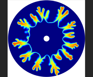



1. Introduction
Flow and transport in porous media occur in a wide variety of situations such as in oil industries (Homsy Reference Homsy1987), carbon dioxide sequestration (Huppert & Neufeld Reference Huppert and Neufeld2014), contamination transport in subsurface aquifers (Welty, Kane & Kauffman Reference Welty, Kane and Kauffman2003), lithium-ion batteries (Chung et al. Reference Chung, Shearing, Brandon, Harris and García2014), hydrogeology (Cardenas et al. Reference Cardenas2019) and biofilms (Davit et al. Reference Davit, Byrne, Osborne, Pitt-Francis, Gavaghan and Quintard2013), to name a few. When a less viscous fluid displaces a more viscous one in porous media, this unfavourable viscosity variation makes the system unstable and causes the displacing fluid to channel through the displaced one (Saffman & Taylor Reference Saffman and Taylor1958). This instability, which is known as viscous fingering (VF), is a fundamental fluid mechanics problem which has important practical applications such as in secondary oil recovery (Homsy Reference Homsy1987), chromatography separation (Rana et al. Reference Rana, Pramanik, Martin, De Wit and Mishra2019) and geothermal reservoir reinjection (Mcdowell, Zarrouk & Clarke Reference Mcdowell, Zarrouk and Clarke2016), to name a few. The first experimental study that reported this instability during the displacement of two miscible fluids in a porous medium was performed by Hill (Reference Hill1952). Several theoretical, computational and experimental studies have followed this seminal work to improve our understanding of the mechanism of VF and its controllability (Sharma et al. Reference Sharma, Nand, Pramanik, Chen and Mishra2020).
The miscible VF occurring in the displacement driven by radial source flows has attracted many researchers due to the large number of laboratory experiments that are performed in radial Hele-Shaw cells as well as the important aspect of spatially dependent base velocity unlike the constant base velocity in rectilinear flow (e.g. Paterson Reference Paterson1981; Tan & Homsy Reference Tan and Homsy1987; Yortsos Reference Yortsos1987; Sharma et al. Reference Sharma, Nand, Pramanik, Chen and Mishra2020, and references therein). The effects of three-dimensional disturbances, velocity-induced dispersion and concentration-dependent diffusion were studied by solving the stability problems using both a linear stability theory and direct numerical simulations (Riaz & Meiburg Reference Riaz and Meiburg2003a,Reference Riaz and Meiburgb; Riaz, Pankiewitz & Meiburg Reference Riaz, Pankiewitz and Meiburg2004). Pritchard (Reference Pritchard2004) revisited the radial fingering problem by considering double-diffusive effects due to heat and mass transfer and investigated the properties of each front contributing to the tendency of the flow instability by expanding the temperature and concentration disturbances as series of orthogonal functions. Linear stability analysis (LSA) and numerical simulations of VF during reinjection in geothermal reservoirs revealed that the key parameters governing the onset of VF instability and the finger structures are the Péclet number, the log-viscosity ratio and the permeability heterogeneity (Mcdowell et al. Reference Mcdowell, Zarrouk and Clarke2016). However, the effects of chemical reactions on the onset and the growth of the VF were not considered.
The effects of chemical reactions on VF instability have attracted the interest of several researchers (see De Wit (Reference De Wit2016, Reference De Wit2020) for recent reviews). Experiments revealed that viscosity changing chemical reactions (Nagatsu et al. Reference Nagatsu, Matsuda, Kato and Tada2007) and precipitation reactions (Nagatsu et al. Reference Nagatsu, Ishii, Tada and De Wit2014) can induce VF in a radial Hele-Shaw cell. In precipitation reaction systems that produced metallic carbonate precipitations (e.g. CaCO $_3$, BaCO
 $_3$), the ratio of the reactants’ concentration (i.e. the initial concentrations of the carbonate and the metallic ions), the species of the metallic ions and the injection flux played important roles in the pattern formation (Schuszter, Brau & De Wit Reference Schuszter, Brau and De Wit2016a,Reference Schuszter, Brau and De Witb; Schuszter & De Wit Reference Schuszter and De Wit2016). Experiments also revealed that the flow pattern controlled the morphology of barium carbonate (BaCO
 $_3$) precipitate particles (Schuszter & De Wit Reference Schuszter and De Wit2016). Very recent experiments captured that the interactions between chemical reactions and hydrodynamic instabilities controlled the morphology of the product and induced new dynamics phenomena (Balog et al. Reference Balog, Bittmann, Schwarzenberger, Eckert, De Wit and Schuszter2019; Escala et al. Reference Escala, De Wit, Carballido-Landeira and Muñuzuri2019).
Nonlinear numerical simulations of rectilinear displacements of  $A + B \rightarrow C$ chemical reaction fronts captured various types of VF motions depending on different combinations of physicochemical parameters (Gérard & De Wit Reference Gérard and De Wit2009; Nagatsu & De Wit Reference Nagatsu and De Wit2011; Nagatsu et al. Reference Nagatsu, Ishii, Tada and De Wit2014). Miscible displacements of reactive fronts in radial flow are scarcely explored theoretically. For example, a theoretical analysis of the properties of reaction–diffusion–advection fronts in the context of an
 $A + B \rightarrow C$ reactive miscible interface subjected to a passive radial advection (Brau, Schuszter & De Wit Reference Brau, Schuszter and De Wit2017) was followed by asymptotic solutions of this miscible reaction–diffusion–advection interface (Trevelyan & Walker Reference Trevelyan and Walker2018).
Recently, theoretical analyses discussed the effects of radial flow with chemical reaction on the solution thickness and dynamics of the reactive front without fingering instability (Brau & De Wit Reference Brau and De Wit2020; Tóth et al. Reference Tóth, Schuszter, Das, Lantos, Horváth, De Wit and Brau2020).
One of the first numerical studies exploring the effects of the reaction rate and the injection flux on the patterns of VF instability in a radial source flow of an  $A + B \rightarrow C$ reactive miscible interface was recently presented by Sharma et al. (Reference Sharma, Pramanik, Chen and Mishra2019). They showed that when the two reactant fluids have the same viscosity, either the inner region or the outer region of the reaction front became unstable when the reaction produced a more or less viscous product. These clearly indicate that the theoretical and numerical studies exploring the effects of chemical reactions on miscible VF in radial flows are very limited and better understandings of the experimental observations await. Specifically, a systematic analysis for understanding the effects of both the hydrodynamics as well as chemistry that incorporates the effects of viscosity mismatch between the reactants remains unexplored.
In the present study, the effects of chemical reaction on the onset of VF during miscible displacement due to the radial source flow in a homogeneous porous medium were analysed with a linear stability theory based on the normal modes analysis and the results are compared with nonlinear simulations (NLS). The stability equations were formulated in a similarity domain and they are solved numerically and also analytically for some specific cases. We asked: How does the physical hydrodynamics in the form of the viscosity ratios of the two reactants,  $R_{A}$ and
 $R_{B}$, influence the reaction-induced fingering dynamics?
We restrict our stability analysis for the limiting case of  $Da \tau \rightarrow \infty$, where
 $Da$ is the Damköhler number and
 $\tau$ is the dimensionless time. They are defined in § 2.1.
Based on the results of the LSA, we extended the numerical work of Sharma et al. (Reference Sharma, Pramanik, Chen and Mishra2019) by considering such physical hydrodynamics effects on the instability patterns. We found that both the LSA and NLS predicted that the critical parameters for instability decay with Péclet number following power-law relations. A novel finding of our current study in this limiting case is that the instability of the system can be explained in the parameter space of two new mobility ratios,  $R_{Phys} = -(R_{A} - \beta R_{B})$ and
 $R_{Chem} = -(R_{C} - R_{B} - R_{A})$. Here,
 $R_{C}$ is the viscosity ratio associated with the product and
 $\beta$ is the initial concentration ratio of reactant species
 $A$ and
 $B$.
The organization of the paper is as follows. In § 2, the governing equations of the full nonlinear problem and the equations of the base state are presented. An analytic solution of the base-state concentration profiles are not attainable for arbitrary values of  $Da$. However, a closed-form expression in terms of linear combinations of one of the reactants and the product concentration is presented with respect to a similarity variable. Further, we present analytic expressions for the base-state concentration profiles of all three species in the limits of no reaction and
 $Da\tau \rightarrow \infty$ for arbitrary values of Péclet number (
 $Pe$). In the asymptotic limit
 $Pe \gg 1$, these base-state profiles are further simplified and are shown graphically. The linearized perturbation equations are derived for performing the LSA in § 3 and their numerical solutions are discussed therein, followed by NLS in § 4. Further the linear stability results are compared with the NLS in § 5 along with conclusions and implications for future research.
2. Mathematical model
We consider flow of incompressible, Newtonian fluids in a two-dimensional porous medium initially filled with a fluid having a species  $B$ dissolved in it and having a concentration
 $C_{B0}$. We inject a solution of the same solvent fluid and a solute
 $A$ of concentration
 $C_{A0}$ radially from a source at
 $r = 0$ with a constant flux
 $Q$ as shown in figure 1. An irreversible second-order chemical reaction occurs between the two chemical species
 $A$ and
 $B$, and produces another species
 $C$:
 \begin{equation} A + B \xrightarrow{k_{r}} C, \end{equation}
where  $k_{r}$ is the rate of the chemical reaction.
Schematic diagram of a reactive system  $A + B \rightarrow C$ considered here.

The governing equations for the conservation of mass and the conservation of momentum, and the advection–diffusion–reaction mass balance equations for the species are (De Wit Reference De Wit2016; Sharma et al. Reference Sharma, Pramanik, Chen and Mishra2019)
 \begin{gather} \boldsymbol{\nabla} \boldsymbol{\cdot} \boldsymbol{U} = 0, \end{gather}
 \begin{gather}\boldsymbol{\nabla} P ={-}\frac{\mu}{K} \boldsymbol{U}, \end{gather}
 \begin{gather}\frac{\partial C_{A}}{\partial t} + \boldsymbol{U} \boldsymbol{\cdot} \boldsymbol{\nabla} C_{A} = D_A \nabla^2{C_{A}} - k_{r} C_{A} C_{B}, \end{gather}
 \begin{gather}\frac{\partial C_{B}}{\partial t} + \boldsymbol{U} \boldsymbol{\cdot} \boldsymbol{\nabla} C_{B} = D_B \nabla^2{C_{B}} - k_{r} C_{A} C_{B}, \end{gather}
 \begin{gather}\frac{\partial C_{C}}{\partial t} + \boldsymbol{U} \boldsymbol{\cdot} \boldsymbol{\nabla} C_{C} = D_C \nabla^2{C_{C}} + k_{r} C_{A} C_{B}, \end{gather}
where  $\boldsymbol {U} = (U, V)$ is the velocity vector,
 $\mu$ the viscosity,
 $K$ the permeability,
 $P$ the pressure,
 $C_i$ the concentration of chemical species
 $i$ and
 $D_i$ the diffusion coefficient of the chemical species
 $i$ (
 $i = A$,
 $B$ and
 $C$).
2.1. Non-dimensionalization
For a radial flow, the equations of motion are best described in polar  $(r, \theta )$ coordinates. We render the above system of equations dimensionless with the following scaling:
 \begin{gather} \tau = \frac{t}{2 {\rm \pi}K/Q}, \quad ( u, v ) = \frac{( U, V )}{Q/2 {\rm \pi}\sqrt{K}}, \end{gather}
 \begin{gather}( a, b, c ) = \frac{( C_{A}, C_{B}, C_{C} )}{C_{A0}}, \quad p = \frac{P}{\bar{\mu}Q/2 {\rm \pi}K}, \quad \mu = \frac{\tilde{\mu}}{\bar{\mu}}, \end{gather}
where  $\sqrt {K}$ is chosen as the characteristic length scale, such that
 $r \mapsto r/\sqrt {K}$. Here,
 $\bar {\mu }$ is the viscosity of the common solvent. Using these, the dimensionless equations can be written as
 \begin{gather} \frac{1}{r}\frac{\partial}{\partial r} ( r u ) + \frac{1}{r}\frac{\partial v}{\partial \theta} = 0, \end{gather}
 \begin{gather}\frac{\partial p}{\partial r} ={-}\mu u, \end{gather}
 \begin{gather}\frac{1}{r} \frac{\partial p}{\partial \theta} ={-}\mu v, \end{gather}
 \begin{gather}\frac{\partial a}{\partial \tau} + \frac{1}{r}\frac{\partial ( r u a )}{\partial r} + \frac{1}{r} \frac{\partial ( v a )}{\partial \theta} = \frac{1}{Pe} \left[ \frac{1}{r} \frac{\partial}{\partial r} \left( r \frac{\partial a}{\partial r} \right) + \frac{1}{r^2} \frac{\partial^2 a}{\partial \theta^2} \right] - Da ab, \end{gather}
 \begin{gather}\frac{\partial b}{\partial \tau} + \frac{1}{r}\frac{\partial ( r u b )}{\partial r} + \frac{1}{r} \frac{\partial ( v b )}{\partial \theta} = \frac{1}{Pe} \left[ \frac{1}{r} \frac{\partial}{\partial r} \left( r \frac{\partial b}{\partial r} \right) + \frac{1}{r^2} \frac{\partial^2 b}{\partial \theta^2} \right] - Da ab, \end{gather}
 \begin{gather}\frac{\partial c}{\partial \tau} + \frac{1}{r}\frac{\partial ( r u c )}{\partial r} + \frac{1}{r} \frac{\partial ( v c )}{\partial \theta} = \frac{1}{Pe} \left[ \frac{1}{r} \frac{\partial}{\partial r} \left( r \frac{\partial c}{\partial r} \right) + \frac{1}{r^2} \frac{\partial^2 c}{\partial \theta^2} \right] + Da ab. \end{gather}
The dimensionless parameters appearing in (2.5) are the Péclet number  $Pe$ and the Damköhler number
 $Da$, which are defined as (Riaz & Meiburg Reference Riaz and Meiburg2003a,Reference Riaz and Meiburgb; Trevelyan & Walker Reference Trevelyan and Walker2018)
 \begin{equation} Pe = \frac{Q}{2 {\rm \pi}D_A} \quad \mbox{and} \quad Da = \frac{2 {\rm \pi}k_{r} C_{A0} K}{Q}. \end{equation}
The Péclet number represents the ratio of the advective transfer rate to the diffusive one, and the Damköhler number represents the ratio of the mass transfer time scale to the reaction time scale. To complete the above model, the viscosity variation with the concentration is assumed to follow an Arrhenius relation:
 \begin{equation} \mu(a, b, c) = \exp ( R_{A} a + R_{B} b + R_{C} c ), \end{equation}
where  $R_{A}$,
 $R_{B}$ and
 $R_{C}$ are the log-viscosity ratios defined as
 \begin{equation} R_{A} = \ln \left( \frac{\mu(1,0,0)}{\mu(0,0,0)} \right), \quad R_{B} = \ln \left( \frac{\mu(0,1,0)}{\mu(0,0,0)} \right), \quad R_{C} = \ln \left( \frac{\mu(0,0,1)}{\mu(0,0,0)} \right). \end{equation}
To focus on the effects of the chemical reaction only, Sharma et al. (Reference Sharma, Pramanik, Chen and Mishra2019) assumed  $R_{A} = R_{B} = 0$, and therefore the physical hydrodynamic effects remained unexplored.
Note that the physicochemical effects on the viscosity profiles for the limiting cases of  $R_A = 0$ and
 $\beta = 1$ are identical to those shown by Hejazi et al. (Reference Hejazi, Trevelyan, Azaiez and De Wit2010).
2.2. Base state
The above equations admit the following base-state axisymmetric solutions. The base-state velocity field is  $( u_0, v_0 ) = ( 1/r, 0 )$, whereas the base concentrations are governed by (Brau et al. Reference Brau, Schuszter and De Wit2017; Trevelyan & Walker Reference Trevelyan and Walker2018)
 \begin{gather} \frac{\partial a_0}{\partial \tau} + \left( 1 - \frac{1}{Pe} \right) \frac{1}{r} \frac{\partial a_0}{\partial r} = \frac{1}{Pe} \frac{\partial^2 a_0}{\partial r^2} - Da a_0 b_0, \end{gather}
 \begin{gather}\frac{\partial b_0}{\partial \tau} + \left( 1 - \frac{1}{Pe} \right) \frac{1}{r} \frac{\partial b_0}{\partial r} = \frac{1}{Pe} \frac{\partial^2 b_0}{\partial r^2} - Da a_0 b_0, \end{gather}
 \begin{gather}\frac{\partial c_0}{\partial \tau} + \left( 1 - \frac{1}{Pe} \right) \frac{1}{r} \frac{\partial c_0}{\partial r} = \frac{1}{Pe} \frac{\partial^2 c_0}{\partial r^2} + Da a_0 b_0, \end{gather}
under the following conditions:
 \begin{gather} \left . \begin{array}{c@{}} a_0 - 1 = b_0 = c_0 = 0 \mbox{ at } r = 0, \\ a_0= b_0 - \beta = c_0 = 0 \mbox{ as } r \rightarrow \infty, \end{array} \right\} \quad \forall \, \tau > 0, \end{gather}
 \begin{gather}a_0 = b_0 - \beta = c_0 = 0 \mbox{ at } \tau = 0, \quad \forall\, r. \end{gather}
Here,  $\beta = C_{B0}/C_{A0}$ is the ratio of the reactants’ initial concentration. Defining (see Appendix A for details)
 \begin{equation} \phi_0 = \frac{a_0 - b_0 + \beta}{1 + \beta} = a_0 + c_0, \end{equation}
the system of (2.9) can be reduced to the following single equation:
 \begin{equation} \frac{\partial \phi_0}{\partial \tau} + \left( 1 - \frac{1}{Pe} \right) \frac{1}{r} \frac{\partial \phi_0}{\partial r} = \frac{1}{Pe} \frac{\partial^2 \phi_0}{\partial r^2}. \end{equation}
Further, the proper initial and boundary conditions are
 \begin{equation} \phi_0(r, 0) = 0, \quad \phi_0(0, \tau) = 1 \quad \mbox{and} \quad \phi_0(\infty, \tau) = 0. \end{equation}
Therefore, the complete base-state concentration for both the reactants and product can be obtained as follows. (i) Solve the initial boundary value problem consisting of a linear advection–diffusion equation and Dirichlet conditions, given by (2.12) and (2.13a–c). (ii) Find the base-state concentration for one of the three species  $A, B$ and
 $C$. (iii) Subsequently, using the relations from (2.11) one can obtain the base-state concentration of the remaining two species. We will see in §§ 2.2.1 and 2.2.2 that for the limiting cases of
 $Da = 0$ and
 $Da^{\ast }$
 $(= Da \tau ) \rightarrow \infty$, we have to solve only one initial boundary value problem for the unknown
 $\phi _0$. For
 $Da^{\ast } < \infty$, one needs to solve two initial boundary value problems – one for the variable
 $\phi _0$ and the other for one of the three species
 $A, B$ and
 $C$ – which is beyond the scope of this paper. Using the identity from (2.11), we obtain
 \begin{equation} \beta a_0 + b_0 + ( 1 + \beta ) c_0 = \beta, \end{equation}
relating the base-state concentration of the species  $A$,
 $B$ and
 $C$. The gradient of the base-state log-viscosity is
 \begin{equation} \frac{\partial \ln \mu_0}{\partial r} = ( R_{A} - \beta R_{B} ) \frac{\partial \phi_0}{\partial r} + ( R_{C} - R_{B} - R_{A} ) \frac{\partial c_0}{\partial r}. \end{equation}
We introduce a similarity transformation  $(r, \tau ) \mapsto (\xi , \tau )$, where the similarity variable is defined as
 $\xi = r^2 Pe /(4 \tau )$. Under this transformation, the steady state of
 $\phi _0$ satisfies
 \begin{equation} \xi \frac{\textrm{d}^2 \phi_0}{\textrm{d} \xi^2} + \left( \xi - \frac{Pe}{2} + 1 \right) \frac{\textrm{d}\phi_0}{\textrm{d}\xi} = 0, \end{equation}
and yields the following similarity solution:
 \begin{equation} \phi_0(\xi) = \frac{\varGamma ( Pe/2, \xi )}{\varGamma ( Pe/2 )} = \gamma ( Pe/2, \xi ). \end{equation}
Here,  $\varGamma ( \alpha , x ) = \int _x^{\infty } t^{\alpha - 1} \textrm {e}^{-t} \textrm {d}t$ is the upper incomplete gamma function,
 $\varGamma ( \alpha )$ is the gamma function and
 $\gamma ( \alpha , x )$ is the regularized upper incomplete gamma function. Combining (2.11) and (2.17), we obtain (Brau et al. Reference Brau, Schuszter and De Wit2017)
 \begin{equation} a_0 - b_0 ={-}\beta + ( 1 + \beta ) \gamma ( Pe/2, \xi ). \end{equation}
It is to be noted that the displacing front ( $\xi = Pe/2$) is different from the reaction front (
 $\xi _R$), which can be obtained by setting
 $a_0 - b_0 = 0$ in (2.18) and solving for
 $\xi$ yielding
 \begin{equation} \gamma ( Pe/2, \xi_R ) = \frac{\beta}{1 + \beta}. \end{equation}
Note that (2.16) is similar to (41) of Tan & Homsy (Reference Tan and Homsy1987) barring that  $Pe/2$ in the former is replaced by
 $Pe$ in the latter. Since we write the base-state concentration of the species in terms of
 $\phi _0(\xi )$ and our LSA is performed in terms of the similarity variable
 $\xi$, we will see in § 3 that the stiff nature of the stability equations becomes a problem for large
 $Pe$ as explained by Tan & Homsy (Reference Tan and Homsy1987). Therefore, following Tan & Homsy (Reference Tan and Homsy1987) we present our LSA for three different cases of
 $Pe$: (i) general values of
 $Pe$ up to
 $O(10)$, (ii) moderate
 $Pe$ (
 $Pe \gg 1$) and (iii) asymptotically large
 $Pe$ (
 $Pe \rightarrow \infty$).
For  $Pe \gg 1$, (2.17) reduces to
 \begin{equation} \phi_0(\zeta) = \tfrac{1}{2} \mbox{erfc}(\zeta) + O( P\textrm{e}^{{-}1/2} ), \end{equation}
where  $\zeta = ( \xi - Pe/2 )/\sqrt {Pe}$ and hence
 $\zeta = 0$ is the displacing front. For
 $Pe \geqslant 20$, (2.20) approximates (2.17) quite well (Tan & Homsy Reference Tan and Homsy1987; Kim Reference Kim2012). The reaction front
 $\zeta _R$, at which we have
 $a_0(\zeta _R) = b_0(\zeta _R)$, can be approximated as
 \begin{equation} \zeta_R = \mbox{erfc}^{{-}1}\left( \frac{2 \beta}{1 + \beta} \right). \end{equation}
The physical and chemical fronts, i.e. the displacing and the reaction fronts, coincide if and only if  $\beta = 1$.
2.2.1. Non-reactive case ( $Da = 0$)

In the non-reactive case ( $Da = 0$), no product is formed (
 $c_0 = 0$) and we have
 $Da^{\ast } = 0$. Therefore, from (2.11) and (2.15) we obtain
 \begin{gather} ( a_0, b_0 ) = ( \phi_0, \beta ( 1 - \phi_0 ) ), \end{gather}
 \begin{gather}\frac{\partial \ln \mu_0}{\partial r} = ( R_{A} - \beta R_{B} ) \frac{\partial \phi_0}{\partial r}. \end{gather}
Because in this limit the chemical reaction plays no role in the viscosity distribution, we define  $R_{Phys} = -( R_{A} - \beta R_{B} )$, and this limit of
 $Da^{\ast }$ will be used to analyse the case of non-reactive displacements (Kim Reference Kim2012).
2.2.2. Case of $Da^{\ast } \rightarrow \infty$

For the limiting cases of  $Da^{\ast } \rightarrow \infty$, such as CaCO
 $_3$ and BaCO
 $_3$ precipitation systems considered in Schuszter & De Wit (Reference Schuszter and De Wit2016), the two reactants do not coexist, i.e.
 $a_0(\xi \geqslant \xi _R) = 0$ and
 $b_0(\xi < \xi _R) = 0$. Therefore, the base concentration fields and the gradient of the log-viscosity can be obtained as
 \begin{gather} ( a_0, b_0, c_0 ) = \left\{ \begin{array}{@{}ll} ( (1 + \beta)\phi_0 - \beta, 0, \beta(1 - \phi_0) ) & \mbox{for } \xi \leqslant \xi_R, \\ ( 0 , \beta - (1+\beta)\phi_0, \phi_0 ) & \mbox{for } \xi > \xi_R , \end{array} \right. \end{gather}
 \begin{gather}\frac{\partial \ln \mu_0}{\partial r} = \left\{ \begin{array}{@{}ll} -( R_{Phys} - \beta R_{Chem} ) \dfrac{\partial \phi_0}{\partial r} & \mbox{for } \xi \leqslant \xi_R, \\ -( R_{Phys}+ R_{Chem} ) \dfrac{\partial \phi_0}{\partial r} & \mbox{for } \xi > \xi_R , \end{array} \right. \end{gather}
where  $R_{Chem} = - ( R_{C} - R_{B} - R_{A} )$.
The base concentration profiles given in (2.20) and (2.23a) are plotted in figure 2 with respect to the transformed self-similar variable  $\zeta$ for
 $\beta < 1$,
 $\beta = 1$ and
 $\beta > 1$. This figure depicts, as expected by the construction of the new variable
 $\zeta$, that the displacing front,
 $\zeta = 0$, is universal with respect to
 $\beta$. It also confirms that the reaction front depends on
 $\beta$ and it is different from the displacing front for
 $\beta \neq 1$. When the reactant species
 $A$ and
 $B$ have the same initial concentration (
 $\beta = 1$), the reaction front is the same as the displacing front and the product concentration becomes symmetric about this front (see figure 2b). On the other hand, when one of the reactant species is more concentrated than the other (i.e.
 $\beta > 1$ or
 $\beta < 1$), their diffusive fluxes are different, which results in an asymmetry behaviour of the displacing front. For
 $\beta \neq 1$, the reaction front and hence greater amount of product are situated in the region that is rich in the less concentrated species. Figures 2(a) and 2(c) depict that the reaction front is situated in the
 $B$-rich and
 $A$-rich regions, respectively, for
 $\beta < 1$ and
 $\beta > 1$. Depending upon these base-state concentration profiles, the VF instability can occur when the less viscous reactant
 $A$ pushes the more viscous product
 $C$, or less viscous product
 $C$ displaces the more viscous reactant
 $B$, or both. In the following sections, we present LSA as well as NLS for understanding these reactive VF instability cases.
Base-state concentrations  $a_0(\zeta ), b_0(\zeta )$ and
 $c_0(\zeta )$ along with
 $\phi _0(\zeta )$ are plotted in the limiting case of
 $Da^{\ast } \rightarrow \infty$ for different values of
 $\beta < 1$,
 $\beta = 1$ and
 $\beta > 1$: (a)
 $\beta = 0.5$, (b)
 $\beta = 1$ and (c)
 $\beta = 1.5$.

Since  $\partial \phi _0/\partial r$ is always negative regardless of
 $Da^{\ast }$, (2.23b) suggests that the instabilities of the inner and the outer interfaces of the product depend on the sign of
 $R_{Phys} - \beta R_{Chem}$ and
 $R_{Phys} + R_{Chem}$, respectively. In short, we expect inward and outward fingers at the inner and outer interfaces of the product when the inequalities
 \begin{gather} R_{Chem} < R_{Phys}/\beta, \end{gather}
 \begin{gather}R_{Chem} >{-}R_{Phys} \end{gather}
are satisfied, respectively. These stability conditions are equivalent to  $R_{C} > R_{A} ( 1 + \beta )/\beta$ and
 $R_{C} < R_{B} ( 1 + \beta )$, respectively. Note that both the inequalities hold simultaneously only when
 $R_{Phys} > 0$. In such cases, both the inward and outward fingers may appear when
 $-R_{Phys} < R_{Chem} < R_{Phys}/\beta$, or equivalently,
 $R_{A} (1 + \beta )/\beta < R_{C} < R_{B} (1 + \beta )$.
3. Linear stability analysis
3.1. Stability equations
Under the LSA, we introduce infinitesimal disturbances around the base-state solutions, such that  $u = u_0 + u_1$,
 $v = v_0 + v_1$,
 $p = p_0 + p_1$,
 $a = a_0 + a_1$,
 $b = b_0 + b_1$,
 $c = c_0 + c_1$, where the subscripts ‘0’ and ‘1’ correspond to the base state and the disturbance quantities, respectively. The resulting perturbed equations are
 \begin{gather} \frac{1}{r} \frac{\partial}{\partial r}( r u_1 ) + \frac{1}{r} \frac{\partial v_1}{\partial \theta} = 0, \end{gather}
 \begin{gather}\frac{\partial p_1}{\partial r} ={-}\mu_0 u_1 - \frac{1}{r} \left[ \left( \frac{\partial \mu}{\partial a} \right)_{(a_0, b_0, c_0)} a_1 + \left( \frac{\partial \mu}{\partial b} \right)_{(a_0, b_0, c_0)} b_1 + \left( \frac{\partial \mu}{\partial c} \right)_{(a_0, b_0, c_0)} c_1 \right], \end{gather}
 \begin{gather}\frac{1}{r} \frac{\partial p_1}{\partial \theta} ={-}\mu_0 v_1, \end{gather}
 \begin{gather}\frac{\partial a_1}{\partial \tau} + \frac{1}{r} \frac{\partial a_1}{\partial r} + \frac{\partial a_0}{\partial r}u_1 = \frac{1}{Pe} \left[ \frac{1}{r} \frac{\partial}{\partial r} \left( r \frac{\partial a_1}{\partial r} \right) + \frac{1}{r^2} \frac{\partial^2 a_1}{\partial \theta^2} \right] - Da ( a_0 b_1 + a_1 b_0 ), \end{gather}
 \begin{gather}\frac{\partial b_1}{\partial \tau} + \frac{1}{r} \frac{\partial b_1}{\partial r} + \frac{\partial b_0}{\partial r}u_1 = \frac{1}{Pe} \left[ \frac{1}{r} \frac{\partial}{\partial r} \left( r \frac{\partial b_1}{\partial r} \right) + \frac{1}{r^2} \frac{\partial^2 b_1}{\partial \theta^2} \right] - Da ( a_0 b_1 + a_1 b_0 ), \end{gather}
 \begin{gather}\frac{\partial c_1}{\partial \tau} + \frac{1}{r} \frac{\partial c_1}{\partial r} + \frac{\partial c_0}{\partial r}u_1 = \frac{1}{Pe} \left[ \frac{1}{r} \frac{\partial}{\partial r} \left( r \frac{\partial c_1}{\partial r} \right) + \frac{1}{r^2} \frac{\partial^2 c_1}{\partial \theta^2} \right] + Da ( a_0 b_1 + a_1 b_0 ). \end{gather}
The corresponding boundary conditions are
 \begin{gather} r u_1 \rightarrow 0, \quad a_1 \rightarrow 0, \quad b_1 \rightarrow 0 \quad \mbox{and} \quad c_1 \rightarrow 0 \mbox{ as } r \rightarrow 0, \end{gather}
 \begin{gather}u_1 \rightarrow 0, \quad a_1 \rightarrow 0, \quad b_1 \rightarrow 0 \quad \mbox{and} \quad c_1 \rightarrow 0 \mbox{ as } r \rightarrow \infty. \end{gather}
Eliminating pressure and the azimuthal velocity component, the linear stability equations (3.1a)–(3.1c) reduce to
 \begin{align} & \frac{\partial^2 \psi_1}{\partial r^2} + \left( \frac{1}{r} + R_{A} \frac{\partial a_0}{\partial r} + R_{B} \frac{\partial b_0}{\partial r} + R_{C} \frac{\partial c_0}{\partial r} \right) \frac{\partial \psi_1}{\partial r} + \frac{1}{r^2} \frac{\partial^2 \psi_1}{\partial \theta^2} \nonumber\\ & \quad ={-}\frac{1}{r^2} \frac{\partial^2}{\partial \theta^2} ( R_{A} a_1 + R_{B} b_1 + R_{C} c_1 ), \end{align}
where  $\psi _1 = r u_1$. In the spirit of
 $\phi _0$ defined in (2.11), we define
 \begin{equation} \phi_1 = \frac{a_1 - b_1}{1 + \beta} = a_1 + c_1 ={-}\frac{b_1 + c_1}{\beta}, \end{equation}
such that (3.1d)–(3.1f) can be reduced to a single advection–diffusion equation:
 \begin{equation} \frac{\partial \phi_1}{\partial \tau} + \frac{1}{r} \frac{\partial \phi_1}{\partial r} + \frac{\partial \phi_0}{\partial r}u_1 = \frac{1}{Pe} \left[ \frac{1}{r} \frac{\partial}{\partial r} \left( r \frac{\partial \phi_1}{\partial r} \right) + \frac{1}{r^2} \frac{\partial^2 \phi_1}{\partial \theta^2} \right]. \end{equation}
The proper boundary conditions associated with (3.3) and (3.5) are
 \begin{gather} \psi_1 = \phi_1 = 0 \mbox{ at } r = 0, \end{gather}
 \begin{gather}\psi_1 \rightarrow 0 \quad \mbox{and} \quad \phi_1 \rightarrow 0 \mbox{ as } r \rightarrow \infty. \end{gather}
From (3.4), we get the following auxiliary relation:
 \begin{equation} \beta a_1 + b_1 + ( 1 + \beta ) c_1 = 0. \end{equation}
Using the similarity transformation introduced in § 2,  $(r, \tau ) \mapsto (\xi , \tau )$, where the similarity variable is defined as
 $\xi = Pe ( r^2/4 \tau )$, (3.3) and (3.5) are transformed into
 \begin{align} & \frac{\partial}{\partial \xi} \left( \xi \frac{\partial \psi_1}{\partial \xi} \right) + \left( R_{A} \frac{\partial a_0}{\partial \xi} + R_{B} \frac{\partial b_0}{\partial \xi} +R_{C} \frac{\partial c_0}{\partial \xi} \right) \xi \frac{\partial \psi_1}{\partial \xi} + \frac{1}{4 \xi} \frac{\partial^2 \psi_1}{\partial \theta^2} \nonumber\\ & \quad ={-} \frac{1}{4 \xi} \frac{\partial^2}{\partial \theta^2} ( R_{A} a_1 + R_{B} b_1 + R_{C} c_1 ), \end{align}
 \begin{align} & \tau \frac{\partial \phi_1}{\partial \tau} = \mathcal{L}_{\xi} \phi_1 + \frac{1}{4 \xi} \frac{\partial^2 \phi_1}{\partial \theta^2} - \frac{1}{2} Pe \frac{\textrm{d} \phi_0}{\textrm{d} \xi} \psi_1, \end{align}
respectively. Here, the differential operator  $\mathcal {L}_{\xi }$ is defined as
 \begin{equation} \mathcal{L}_{\xi} = \frac{\partial}{\partial \xi} \left( \xi \frac{\partial}{\partial \xi} \right) + \left( \xi - \frac{Pe}{2} \right) \frac{\partial}{\partial \xi}. \end{equation}
For the limiting case of  $Pe \gg 1$, (3.8) become
 \begin{align} & \frac{\partial^2 \psi^{{\ast}}_1}{\partial \zeta^2} + \left( R_{A} \frac{\partial a_0}{\partial \zeta} + R_{B} \frac{\partial b_0}{\partial \zeta} +R_{C} \frac{\partial c_0}{\partial \zeta} \right) \frac{\partial \psi^{{\ast}}_1}{\partial \zeta} + \frac{1}{Pe} \frac{\partial^2 \psi^{{\ast}}_1}{\partial \theta^2} \nonumber\\ & \quad ={-} \frac{1}{Pe} \frac{\partial^2}{\partial \theta^2} ( R_{A}^{{\ast}} a_1 + R_{B}^{{\ast}} b_1 + R_{C}^{{\ast}} c_1 ) + O ( P\textrm{e}^{{-}1/2} ), \end{align}
 \begin{align} & 2 \tau \frac{\partial \phi_1}{\partial \tau} = \mathcal{L}_{\zeta} \phi_1 + \frac{1}{Pe} \frac{\partial^2 \phi_1}{\partial \theta^2} - \frac{\textrm{d} \phi_0}{\textrm{d} \zeta} \psi^{{\ast}}_1 + O ( P\textrm{e}^{{-}1/2} ), \end{align}
where
 \begin{equation} \mathcal{L}_{\zeta} = \frac{\partial^2}{\partial \zeta^2} + 2 \zeta \frac{\partial}{\partial \zeta} \end{equation}
and  $\psi ^{\ast }_1 = \psi _1 \sqrt {Pe}$,
 $R_{A}^{\ast } = R_{A} \sqrt {Pe}$,
 $R_{B}^{\ast } = R_{B} \sqrt {Pe}$ and
 $R_{C}^{\ast } = R_{C} \sqrt {Pe}$.
In the remainder of this section, we discuss linear stability in the limit  $Da^{\ast } \rightarrow \infty$ (see Appendix B for the non-reactive case, i.e.
 $Da^{\ast } = 0$). In this limit, both the advection and the diffusion terms remain significant in (3.1d)–(3.1f), provided
 \begin{equation} a_0 b_1 + a_1 b_0 = 0. \end{equation}
Recall that for  $Da^{\ast } \rightarrow \infty$, we have
 $a_0(\xi \geqslant \xi _R) = 0$ and
 $b_0(\xi < \xi _R) = 0$. Combining this with (3.12), we obtain
 $a_1 ( \xi \geqslant \xi _R ) = 0$ and
 $b_1 ( \xi < \xi _R ) = 0$. Hence, using (3.4), the concentration disturbance fields can be obtained as
 \begin{equation} ( a_1, b_1, c_1 ) = \left\{ \begin{array}{@{}ll} ( (1+\beta)\phi_1, 0, -\beta \phi_1 ) & \mbox{for } 0 \leqslant \xi \leqslant \xi_R \\ ( 0, -(1 + \beta)\phi_1, \phi_1 ) & \mbox{for } \xi > \xi_R . \end{array} \right. \end{equation}
In this limit, (3.8a) becomes
 \begin{align} & \frac{\partial}{\partial \xi} \left( \xi \frac{\partial \psi_1}{\partial \xi} \right) - ( R_{Phys} - \beta R_{Chem} ) \frac{\textrm{d} \phi_0}{\textrm{d} \xi} \xi \frac{\partial \psi_1}{\partial \xi} + \frac{1}{4 \xi} \frac{\partial^2 \psi_1}{\partial \theta^2} \nonumber\\ & \quad = ( R_{Phys} - \beta R_{Chem} ) \frac{1}{4 \xi} \frac{\partial^2 \phi_1}{\partial \theta^2} \quad \mbox{for } \xi \leqslant \xi_R,\end{align}
 \begin{align} & \frac{\partial}{\partial \xi} \left( \xi \frac{\partial \psi_1}{\partial \xi} \right) - ( R_{Phys} + R_{Chem} ) \frac{\textrm{d} \phi_0}{\textrm{d} \xi} \xi \frac{\partial \psi_1}{\partial \xi} + \frac{1}{4 \xi} \frac{\partial^2 \psi_1}{\partial \theta^2} \nonumber\\ & \quad = ( R_{Phys} + R_{Chem} ) \frac{1}{4 \xi} \frac{\partial^2 \phi_1}{\partial \theta^2} \quad \mbox{for } \xi > \xi_R. \end{align}
Similarly, (3.10a) becomes
 \begin{align} & \frac{\partial^2 \psi^{{\ast}}_1}{\partial \zeta^2} - ( R_{Phys} - \beta R_{Chem} ) \frac{\textrm{d} \phi_0}{\textrm{d} \zeta} \frac{\partial \psi^{{\ast}}_1}{\partial \zeta} + \frac{1}{Pe} \frac{\partial^2 \psi^{{\ast}}_1}{\partial \theta^2} \nonumber\\ & \quad = ( R_{Phys}^{{\ast}} - \beta R_{Chem}^{{\ast}} ) \frac{1}{Pe} \frac{\partial^2 \phi_1}{\partial \theta^2} + O ( P\textrm{e}^{{-}1/2} ) \quad \mbox{for } \zeta \leqslant \zeta_R, \end{align}
 \begin{align} & \frac{\partial^2 \psi^{{\ast}}_1}{\partial \zeta^2} - ( R_{Phys} + R_{Chem} ) \frac{\textrm{d} \phi_0}{\textrm{d} \zeta} \frac{\partial \psi^{{\ast}}_1}{\partial \zeta} + \frac{1}{Pe} \frac{\partial^2 \psi^{{\ast}}_1}{\partial \theta^2} \nonumber\\ & \quad = ( R_{Phys}^{{\ast}} + R_{Chem}^{{\ast}} ) \frac{1}{Pe} \frac{\partial^2 \phi_1}{\partial \theta^2} + O ( P\textrm{e}^{{-}1/2} ) \quad \mbox{for } \zeta > \zeta_R. \end{align}
Here,  $R_{Phys}^{\ast } = R_{Phys} \sqrt {Pe}$ and
 $R_{Chem}^{\ast } = R_{Chem} \sqrt {Pe}$. The corresponding boundary conditions associated with (3.8b) (or (B2) for
 $Da^{\ast } = 0$) and (3.14) are
 \begin{gather} \psi_1 = \phi_1 = 0 \mbox{ at } \xi = 0, \end{gather}
 \begin{gather} \psi_1 \rightarrow 0 \quad \mbox{and} \quad \phi_1 \rightarrow 0 \mbox{ as } \xi \rightarrow \infty, \end{gather}
whereas the boundary conditions associated with (3.10b) (or (B3) for  $Da^{\ast } = 0$) and (3.15) are
 \begin{gather} \psi^{{\ast}}_1 = 0 \quad \mbox{and} \quad \phi_1 = 0 \mbox{ at } \zeta ={-} \sqrt{Pe}/2, \end{gather}
 \begin{gather}\psi^{{\ast}}_1 \rightarrow 0 \quad \mbox{and} \quad \phi_1 \rightarrow 0 \mbox{ as } \zeta \rightarrow \infty. \end{gather}
3.2. Normal mode analysis
Since the coefficients of (3.8b) (or (B2) for  $Da^{\ast } = 0$) and (3.14) are independent of
 $\tau$ and
 $\theta$, under the normal mode analysis (Tan & Homsy Reference Tan and Homsy1987), the perturbation quantities
 $\phi _1$ and
 $\psi _1$ are expressed as
 \begin{gather} \phi_1(\xi, \theta, \tau) = \varPhi ( \xi ) \textrm{e}^{\textrm{i} n \theta} \tau^{\sigma}, \end{gather}
 \begin{gather}\psi_1(\xi, \theta, \tau) = \varPsi ( \xi ) \textrm{e}^{\textrm{i} n \theta} \tau^{\sigma}, \end{gather}
where  $n$ is the azimuthal wavenumber and growth exponent
 $\sigma$ is defined as
 $\tau ({\partial \phi _1}/{\partial \tau }) = \sigma \phi _1$. Using this normal mode decomposition, (3.8b) becomes
 \begin{equation} \sigma \varPhi = \mathcal{L}_{\xi} \varPhi - \frac{n^2}{4 \xi} \varPhi - \frac{1}{2} Pe \frac{\textrm{d}\phi_0}{\textrm{d} \xi} \varPsi, \end{equation}
associated with the equation for the velocity disturbance field:
 \begin{align}
&\frac{\textrm{d}}{\textrm{d} \xi} \left( \xi
\frac{\textrm{d} \varPsi}{\textrm{d} \xi} \right) - (
R_{Phys} - \beta R_{Chem} ) \frac{\textrm{d}
\phi_0}{\textrm{d} \xi} \xi \frac{\textrm{d}
\varPsi_1}{\textrm{d} \xi} - \frac{n^2}{4 \xi} \varPsi
\nonumber\\ & \quad ={-} ( R_{Phys} - \beta R_{Chem} )
\frac{n^2}{4 \xi} \varPhi \quad \mbox{for } \xi \leqslant
\xi_R, \end{align}
 \begin{align}
& \frac{\textrm{d}}{\textrm{d} \xi} \left( \xi \frac{\textrm{d}
\varPsi}{\textrm{d} \xi} \right) - ( R_{Phys} + R_{Chem} )
\frac{\textrm{d} \phi_0}{\textrm{d} \xi} \xi
\frac{\textrm{d} \varPsi_1}{\textrm{d} \xi} - \frac{n^2}{4
\xi} \varPsi \nonumber\\ &\quad ={-} ( R_{Phys} + R_{Chem} )
\frac{n^2}{4 \xi} \varPhi \quad \mbox{for } \xi > \xi_R.
\end{align}
The boundary conditions corresponding to (3.19)–(3.20) are
 \begin{equation} \varPsi \rightarrow 0 \quad \mbox{and} \quad \varPhi \rightarrow 0, \mbox{ as } \xi \rightarrow \pm \infty. \end{equation}
Similarly, for  $Pe \gg 1$, we can apply normal mode analysis as discussed below. Since the coefficients of the stability (3.10b), (B3) and (3.15) are independent of
 $\tau$ and
 $\theta$, the normal mode decomposition of
 $\psi ^{\ast }_1$ reads
 \begin{equation} \psi^{{\ast}}_1(\zeta, \theta, \tau) = \Psi^{{\ast}} ( \zeta ) \textrm{e}^{\textrm{i} n \theta} \tau^{\sigma}, \end{equation}
where  $\varPsi (\xi )$ and
 $\Psi ^{\ast }(\zeta )$ satisfy
 $\Psi ^{\ast } = \varPsi \sqrt {Pe}$. Using this normal mode decomposition for
 $\psi ^{\ast }_1$, along with that for
 $\phi _1$ given in (3.18a), the stability equations become
 \begin{equation} \sigma \varPhi = \frac{1}{2} \left( \mathcal{L}_{\zeta} - \frac{n^2}{Pe} \right) \varPhi - \frac{1}{2} \frac{\textrm{d}\phi_0}{\textrm{d} \zeta} \Psi^{{\ast}}, \end{equation}
associated with
 \begin{gather} \frac{\textrm{d}^2 \Psi^{{\ast}}}{\textrm{d} \zeta^2} - ( R_{Phys} - \beta R_{Chem} ) \frac{\textrm{d} \phi_0}{\textrm{d} \zeta} \frac{\textrm{d} \Psi^{{\ast}}}{\textrm{d} \zeta} - \frac{n^2}{Pe} \Psi^{{\ast}} ={-} \frac{n^2}{Pe} ( R_{Phys}^{{\ast}} - \beta R_{Chem}^{{\ast}} ) \varPhi \quad \mbox{for } \zeta \leqslant \zeta_R, \end{gather}
 \begin{gather}\frac{\textrm{d}^2 \Psi^{{\ast}}}{\textrm{d} \zeta^2} - ( R_{Phys} + R_{Chem} ) \frac{\textrm{d} \phi_0}{\textrm{d} \zeta} \frac{\textrm{d} \Psi^{{\ast}}}{\textrm{d} \zeta} - \frac{n^2}{Pe} \Psi^{{\ast}} ={-} \frac{n^2}{Pe} ( R_{Phys}^{{\ast}} + R_{Chem}^{{\ast}} ) \varPhi \quad \mbox{for } \zeta > \zeta_R. \end{gather}
The boundary conditions corresponding to (3.23)–(3.24) are
 \begin{equation} \Psi^{{\ast}} \rightarrow 0 \quad \mbox{and} \quad \varPhi \rightarrow 0, \mbox{ as } \zeta \rightarrow \pm \infty. \end{equation}
As mentioned in the introduction, contrary to its rectilinear counterpart, theoretical and numerical studies exploring the effects of chemical reactions for miscible VF in radial flows await understanding. In a rectilinear flow, the onset time of instability is captured in terms of frozen time-dependent growth rate using a quasi-steady-state approximation (Hejazi et al. Reference Hejazi, Trevelyan, Azaiez and De Wit2010). It is widely accepted that a quasi-steady-state approximation has its own limitation in the linear stability theory (Kim & Choi Reference Kim and Choi2011) and the same can be overcome by performing the stability analysis in a suitably defined similarity domain (Ben, Demekhin & Chang Reference Ben, Demekhin and Chang2002). In the present study, we have used a similarity transformation and have focused on capturing the critical parameters for the instability using asymptotic instability criterion ( $\tau \rightarrow \infty$) as follows. From (3.18a) and (3.18b), it is clear that the perturbations decay to zero as
 $\tau \rightarrow \infty$ when
 $\sigma < 0$; whereas they grows to infinity as
 $\tau \rightarrow \infty$ when
 $\sigma > 0$. A system is said to be asymptotically stable in the former case, and asymptotically unstable in the latter case (Drazin & Reid Reference Drazin and Reid2004; Chandrasekhar Reference Chandrasekhar2013). Therefore, the critical parameters corresponding to the linear stability theory are computed for
 $Da^* (= Da\tau ) \rightarrow \infty$. We demarcate the parameter space as stable and unstable corresponding to which
 $\sigma < 0$ and
 $\sigma > 0$, respectively. The boundary between these two regions indicates the critical parameters for the onset of instability. Furthermore, a radial flow is significantly different from a rectilinear flow and the LSAs in these two configurations have some critical differences (Tan & Homsy Reference Tan and Homsy1987). For brevity, we do not present any direct comparison between rectilinear and radial flows.
3.2.1. Shooting method
In general, in order to integrate the stability (3.19)–(3.20), a trial value of the eigenvalue  $\sigma$ and that of
 $\textrm {d}\varPsi /\textrm {d}\xi$,
 $\varTheta$ and
 $\textrm {d}\varTheta /\textrm {d}\xi$ at
 $\xi = \xi _R$ are assumed properly for given values of
 $R$,
 $n$ and
 $Pe$ (Kim Reference Kim2018). Since the boundary conditions (3.16) are all homogeneous, the value of
 $\varPsi$ at
 $\xi = \xi _R$ can be assigned arbitrarily. This procedure is based on the shooting method in which the boundary value problem is transformed into the initial value problem. The initial value problem is integrated numerically using the fourth-order Runge–Kutta method. Numerical shooting is done on both sides of the reaction front,
 $\xi = \xi _R$, i.e.
 $0 \leqslant \xi \leqslant \xi _R$ and
 $\xi _R \leqslant \xi < \infty$, such that the boundary conditions (3.16) are satisfied respectively in these two regions. On the right of the injection front, we enforce the boundary conditions (3.16b) to satisfy on a fictitious outer boundary. We use Newton–Raphson iteration to iteratively correct the trial values of
 $\sigma$,
 $\textrm {d}\varPsi /\textrm {d}\xi$,
 $\varTheta$ and
 $\textrm {d}\varTheta /\textrm {d}\xi$ at
 $\xi = \xi _R$ until the linear stability equations satisfy the boundary conditions (3.16) within a relative tolerance of
 $10^{-10}$. Then by increasing the fictitious outer boundary step by step, the above integration is repeated. Finally, the value of
 $\sigma$ is decided through extrapolation.
3.2.2. Spectral analysis
Following Pritchard (Reference Pritchard2004) and Kim (Reference Kim2012), here we obtain an analytic solution for the limiting case of  $Pe \rightarrow \infty$,
 $R_{Phys} \ll 1$ and
 $R_{Chem} \ll 1$, but finite
 $R_{Phys}^{\ast } = R_{Phys} \sqrt {Pe}$ and
 $R_{Chem}^{\ast }= R_{Chem} \sqrt {Pe}$. Under the Sturm–Liouville theory (Al-Gwaiz Reference Al-Gwaiz2008),
 $\varPhi$ can be expressed as
 \begin{equation} \varPhi ( \zeta ) = \sum_{i = 0}^{\infty} A_i \alpha_i \phi_i ( \zeta ), \end{equation}
where  $\phi _i( \zeta )$ are the eigenfunctions of the Sturm–Liouville equation,
 \begin{equation} \mathcal{L}_{\zeta} \phi_i ={-}2 \lambda_i \phi_i. \end{equation}
The solutions of the above equation are weighted  $i$th Hermite polynomials:
 \begin{equation} \phi_i ( \zeta ) = \textrm{e}^{-\zeta^2} H_i ( \zeta ) \quad \mbox{and} \quad i = ( \lambda_i - 1 ) = 0, 1, 2, \ldots \end{equation}
Here, the normalization factors  $\alpha _i$ are
 \begin{equation} \alpha_i = ( \sqrt{\rm \pi} 2^i \mathcal{G} ( i+1 ) )^{{-}1/2}, \quad i = ( \lambda_i - 1 ) = 0, 1, 2, \ldots \end{equation}
Combining (B5) (or equations (3.24)) with (3.26), it can be shown that  $\Psi ^{\ast } ( \zeta )$ follows a series expansion with the same coefficients as
 $\varPhi ( \zeta )$, and the former can be expressed as
 \begin{equation} \Psi^{{\ast}} ( \zeta ) = \sum_{i =0}^{\infty} A_i \alpha_i \psi_i ( \zeta ), \end{equation}
where  $\psi _i$ can be obtained by solving (
 $R_{Phys}, R_{Chem} \ll 1$)
 \begin{gather} \frac{\textrm{d}^2 \psi^{-}_i}{\textrm{d} \zeta^2} - k^2 \psi^{-}_i ={-}k^2 ( R_{Phys}^{{\ast}} - \beta R_{Chem}^{{\ast}} ) \textrm{e}^{-\zeta^2} H_i ( \zeta ) \quad \mbox{for } \zeta \leqslant \zeta_R, \end{gather}
 \begin{gather}\frac{\textrm{d}^2 \psi^{+}_i}{\textrm{d} \zeta^2} - k^2 \psi^{+}_i ={-}k^2 ( R_{Phys}^{{\ast}} + R_{Chem}^{{\ast}} ) \textrm{e}^{-\zeta^2} H_i ( \zeta ) \quad \mbox{for } \zeta > \zeta_R, \end{gather}
such that
 \begin{gather} \psi_i = \left\{ \begin{array}{@{}ll} \psi^{-}_i, & \zeta \leqslant \zeta_R \\ \psi^{+}_i, & \zeta > \zeta_R \end{array} \right. \quad \mbox{and} \end{gather}
 \begin{gather}\lim_{\zeta \rightarrow \zeta_R+} \psi^{+}_i = \psi^{-}_i ( \zeta_R ). \end{gather}
Here,  $k = n/\sqrt {Pe}$ is the scaled wavenumber. We analytically solve the second-order ordinary differential equation (C5) (or (3.31)) associated with the following boundary conditions:
 $\psi _i \rightarrow 0$ as
 $\zeta \rightarrow \pm \infty$. The solutions are summarized in Appendix C. Substituting the above solutions into (3.23), we obtain an eigenvalue problem:
 \begin{equation} \sigma \boldsymbol{a} = \boldsymbol{B} \boldsymbol{a}, \end{equation}
where
 \begin{gather} B_{mn} ={-}\frac{1}{2} ( 2 \lambda_{m} + k^2 ) \delta_{mn} + \frac{1}{2 \sqrt{\rm \pi}} C_{mn}, \quad m, n = 0, 1, 2, \ldots, \end{gather}
 \begin{gather}C_{mn} = \int_{-\infty}^{\infty} \alpha_m \alpha_n \phi_{m} ( \zeta ) \psi_{n} ( \zeta ) \textrm{d}\zeta, \quad m, n = 0, 1, 2, \ldots, \end{gather}
 \begin{gather}\boldsymbol{a} = \left[ A_0, A_1, A_2, \ldots \right]^\textrm{T}. \end{gather}
The growth rate of the perturbed quantities is bounded from above by the largest eigenvalues of  $\boldsymbol {B}$, i.e.
 \begin{equation} \sigma = \max \left\lbrace \mbox{eig} ( \boldsymbol{B} ) \right\rbrace. \end{equation}
Furthermore, we apply the numerical shooting method, discussed in § 3.2.1, to solve (3.23)–(3.24) and the corresponding boundary conditions (3.25).
3.3. Critical conditions for linear instability
The critical conditions for the linearly unstable modes are determined by analysing the neutral stability curves. For example, the critical values of  $R_{Chem}^{\ast }$ and
 $k$ (i.e.
 $R_{Chem, c}^{\ast }$ and
 $k_c$) are obtained from the neutral curves plotted in the
 $R_{Chem}^{\ast }$–
 $k$ plane. For the limiting case of
 $Pe \rightarrow \infty$, the neutral stability curves obtained by solving (3.23)–(3.25) using both the spectral analysis and the numerical shooting method are plotted in figure 3. This figure depicts that the critical value
 $|R_{Chem, c}^{\ast }|$ decreases as
 $\beta$ increases (e.g.
 $|R_{Chem, c}^{\ast }| = 45.48, 30.70$ and
 $21.93$ for
 $\beta = 1/2, 1$ and
 $2$, respectively), but the critical wavenumber
 $k_c$ does not change significantly with
 $\beta$ and remains near
 $1.30$. Recalling
 $R_{Chem}^{\ast } = R_{Chem} \sqrt {Pe}$ and
 $k = n/\sqrt {Pe}$, we approximate for
 $\beta = 1$,
 $R_{Chem} = 30.70/Pe^{1/2}$ and
 $n_c = 1.30 Pe^{1/2}$ as
 $Pe \rightarrow \infty$. Figure 3 also reveals that the numerical shooting method is in very good agreement with the spectral solutions.
Neutral stability curves obtained using spectral analysis (7-term and 9-term approximations) and numerical shooting method for  $R_{Phys}^{\ast } = 0$,
 $Pe \rightarrow \infty$,
 $Da^{\ast } \rightarrow \infty$, (a)
 $\beta = 1/2$, (b)
 $\beta = 1$ and (c)
 $\beta = 2$. The region above (below) each curve corresponds to the region of instability (stability). The values of
 $|R_{Chem}^{\ast }|$ and
 $k$ corresponding to the lowest point of the curve representing the numerical shooting method denote the critical values for the instability. These are denoted by
 $|R_{Chem, c}^{\ast }|$ and
 $k_c$ and are shown by horizontal and vertical dashed-dotted lines, respectively.

Next, we analyse the effects of  $\beta$ on the the critical values
 $R_{Chem, c}^{\ast }$ in terms of
 $R_{Phys}^{\ast }$ as shown in figure 4. This figure reveals that
 $R_{Chem, c}^{\ast }$ has non-trivial dependences on
 $\beta$ and
 $R_{Phys}^{\ast }$. First, we discuss when the initial concentrations of both the reactants are the same, i.e.
 $\beta = 1$. For
 $\beta = 1$, we have
 $\zeta _R = 0$. In this case, if
 $R_{Chem}^{\ast }$ has a negative value, we denote the eigenfunctions as
 $\psi _{i,n}$ and hence (3.31) can be reduced to
 \begin{gather} \frac{\textrm{d}^2 \psi^{-}_{i, n}}{\textrm{d} \zeta^2} - k^2 \psi^{-}_{i, n} ={-} k^2 \left( R_{Phys}^{{\ast}} - \left\lvert R_{Chem}^{{\ast}} \right\rvert \right) \textrm{e}^{-\zeta^2} H_i ( \zeta ) \quad \mbox{for } \zeta \leqslant 0, \end{gather}
 \begin{gather}\frac{\textrm{d}^2 \psi^{+}_{i, n}}{\textrm{d} \zeta^2} - k^2 \psi^{+}_{i, n} ={-}k^2 \left( R_{Phys}^{{\ast}} + \left\lvert R_{Chem}^{{\ast}} \right\rvert \right) \textrm{e}^{-\zeta^2} H_i ( \zeta ) \quad \mbox{for } \zeta > 0. \end{gather}
Similarly, for positive values of  $R_{Chem}^{\ast }$ we denote the eigenfunctions as
 $\psi _{i, p}$ and from (3.31) one can obtain
 \begin{gather} \frac{\textrm{d}^2 \psi^{-}_{i, p}}{\textrm{d} \zeta^2} - k^2 \psi^{-}_{i, p} ={-}k^2 \left( R_{Phys}^{{\ast}} + \left\lvert R_{Chem}^{{\ast}} \right\rvert \right) \textrm{e}^{-\zeta^2} H_i ( \zeta ) \quad \mbox{for } \zeta \leqslant 0, \end{gather}
 \begin{gather}\frac{\textrm{d}^2 \psi^{+}_{i, p}}{\textrm{d} \zeta^2} - k^2 \psi^{+}_{i, p} ={-}k^2 \left( R_{Phys}^{{\ast}} - \left\lvert R_{Chem}^{{\ast}} \right\rvert \right) \textrm{e}^{-\zeta^2} H_i ( \zeta ) \quad \mbox{for } \zeta > 0. \end{gather}
For the odd-mode instabilities, i.e.  $H_i ( - \zeta ) = -H_i ( \zeta )$,
 $\psi ^{-}_{i, n} = - \psi ^{+}_{i, p}$,
 $\psi ^{-}_{i, p} = -\psi ^{+}_{i, n}$ (see Appendix D for further details), and therefore
 $C_{mn}$ of the negative
 $R_{Chem}^{\ast }$ and the positive
 $R_{Chem}^{\ast }$ have opposite sign. In this case the stability condition is strongly dependent on the sign of
 $R_{Chem}^{\ast }$. Kim (Reference Kim2014) reported that the even modes are more unstable than the odd modes. For the even-mode instabilities, i.e.
 $H_i ( - \eta ) = H_i ( \eta )$,
 $\psi ^{+}_{i, n} = \psi ^{-}_{i, p}$ and
 $\psi ^{-}_{i, n} = \psi ^{+}_{i, p}$, and therefore
 $C_{mn}$ of the negative
 $R_{Chem}^{\ast }$ and the positive
 $R_{Chem}^{\ast }$ cases are the same. In other words, for the limiting case of
 $\beta = 1$, the critical conditions are independent of the sign of
 $R_{Chem}^{\ast }$, as shown in figure 4.
Variation of the critical parameter  $R_{Chem, c}^{\ast }$ with
 $R_{Phys}^{\ast }$ obtained from spectral analysis for
 $Da^{\ast } \rightarrow \infty$,
 $Pe \rightarrow \infty$ and different values of
 $\beta$. For
 $\beta = 1$, positive and negative
 $R_{Chem, c}^{\ast }$ are identical. For
 $\beta \neq 1$, positive and negative
 $R_{Chem, c}^{\ast }$ are not only different, but also have a non-trivial dependence on the sign of
 $R_{Phys}^{\ast }$.

The amount of product generated is proportional to  $\beta$. Therefore, irrespective of the signs of
 $R_{Phys}$ and
 $R_{Chem}$, the displacements become more unstable as
 $\beta$ increases. On the contrary, for fixed values of
 $\beta$, the fingering dynamics exhibits more non-trivial dependencies on
 $R_{Phys}$ and
 $R_{Chem}$. As expected, the dynamics is strongly dependent on the signs of both of these dimensionless parameters. First, we consider the case for which the physical front is neutrally stable, i.e.
 $R_{Phys} = 0$. Therefore, using the inequalities (2.24), it is easy to observe that the outward and the inward fingers are formed for
 $R_{Chem} > 0$ and
 $R_{Chem} < 0$, respectively. It is observed that the critical values
 $R_{Chem, c}^{\ast }$ for different
 $R_{Phys}$ have the same absolute values. However, for the stable (
 $R_{Phys} < 0$) and unstable (
 $R_{Phys} > 0$) physical fronts, the scenario is complex. For example, in the latter case, for
 $-R_{Phys} < R_{Chem} < R_{Phys}/\beta$, both the inward and outward fingering are simultaneously susceptible. With
 $\beta$ increasing, the upper limit of this interval diminishes to zero and hence the length of this interval decreases. Contrary to that, in the former case, a stable displacement is expected for
 $R_{Phys}/\beta < R_{Chem} < -R_{Phys}$. Clearly, the effects of
 $\beta$ on the critical parameter
 $R_{Chem, c}^{\ast }$ are significantly different when
 $R_{Phys}$ changes sign (see figure 4). In summary, we observe that for the case of
 $\beta < 1$, the positive
 $R_{Chem}$ systems are more unstable than the negative
 $R_{Chem}$ ones for
 $R_{Phys} < 0$, and vice versa for
 $R_{Phys} > 0$. This trend is reversed for the case of
 $\beta > 1$. Figure 4 implies that
 $R_{Chem, c}$ is a complex function of
 $\beta$,
 $R_{Phys}$ and
 $Pe$.
Similarly, the critical values of  $R_{Chem}$ and
 $n$ (i.e.
 $R_{Chem, c}$ and
 $n_c$) are obtained for (i) small and moderate values of
 $Pe$ and (ii)
 $Pe \gg 1$ from the numerical shooting solutions of (3.19)–(3.21) and (3.23)–(3.25), respectively. Figure 5(a) depicts the variation of this critical parameter with
 $Pe$ for small and moderate
 $Pe$ as well as
 $Pe \gg 1$. It is observed that for small and moderate
 $Pe$ (i.e.
 $Pe \lesssim 40$), the critical values for the finger formation in the outward-directing fingering system (
 $R_{Chem} > 0$) attain smaller values compared to those corresponding to the inward-directing fingering system (
 $R_{Chem} < 0$). This result is in qualitative agreement with NLS (cf. figures 8 and 9 of Sharma et al. (Reference Sharma, Pramanik, Chen and Mishra2019)). Corresponding to these critical values
 $R_{Chem, c}$, we also plot the critical wavenumber
 $n_c$ in figure 5(b). This figure also depicts that for
 $Pe \gg 1$,
 $R_{Chem, c}$ are visually indistinguishable corresponding to the positive and the negative values of
 $R_{Chem}$, and they follow power-law behaviour
 $R_{Chem, c} \sim Pe^{-1/2}$ obtained in the
 $Pe \rightarrow \infty$ asymptotic limit. Again for
 $Pe \gg 1$, the critical wavenumbers follow the power-law relation obtained in the
 $Pe \rightarrow \infty$ asymptotic limit, i.e.
 $n_c \sim Pe^{1/2}$ as
 $Pe \gg 1$.
Linear stability results obtained for purely chemical systems ( $R_{Phys} = 0$) with
 $\beta = 1$ and
 $Da^{\ast } \rightarrow \infty$ by solving (3.20) and (3.24) (for
 $Pe \gg 1$) using the numerical shooting method. Dependence of the critical parameters (a)
 $R_{Chem, c}$ and (b)
 $n_c$ on
 $Pe$. The straight lines correspond to the asymptotic behaviour of these critical parameters in the limit of
 $Pe \rightarrow \infty$ obtained from the spectral analysis discussed in § 3.2.2.

4. Nonlinear simulations
In § 3, we noted that  $R_{Phys}$ and
 $R_{Chem}$ are the two important parameters controlling fingering instabilities. Although LSA indicates asymptotic instability for infinitesimal perturbations, to explore the nonlinearities of fingering instability numerical simulations of the full nonlinear problem are essential. Equations (2.5) are solved in the Cartesian coordinate system using COMSOL Multiphysics (COMSOL 2019).
It is worth mentioning that COMSOL Multiphysics has been much used in fluid dynamics research over the last decade (Campana & Carvalho Reference Campana and Carvalho2014; Nejati, Dietzel & Hardt Reference Nejati, Dietzel and Hardt2015; Nama, Huang & Costanzo Reference Nama, Huang and Costanzo2017; Lerisson et al. Reference Lerisson, Ledda, Balestra and Gallaire2020). COMSOL Multiphysics can be used as a high-level programming environment to create one's own implementation of problems in question as there may not exist any commercial module in COMSOL to solve such problems (Nama et al. Reference Nama, Huang and Costanzo2017). Similarly in this study, we have also used COMSOL as a high-level programming environment. COMSOL has also been used recently to understand various physical aspects of miscible VF problems using the ‘two-phase Darcy law’ module of fluid flow interface (Sharma, Pramanik & Mishra Reference Sharma, Pramanik and Mishra2016, Reference Sharma, Pramanik and Mishra2017; Kumar & Mishra Reference Kumar and Mishra2019). Although this module works well for understanding classical miscible VF problems, it cannot be used to include chemical reactions in a very convenient manner. Therefore, we adopt a different model formalism and model the fluid flow using the ‘Darcy's law module’, which is coupled with the ‘transport of dilute species module’ for the transport of the reactants  $A$ and
 $B$ and the product
 $C$. The former describes a single-phase incompressible fluid dynamics in a porous medium, while the latter considers an advection–diffusion–reaction equation for a scalar species. These coupled nonlinear partial differential equations are solved in an annular region
 $\varOmega = \{(x, y) : r_{in} \leqslant \sqrt {x^2 + y^2} \leqslant r_{out}\}$, where
 $r_{out}$ is the outer radius of the annulus and
 $r_{in}$ is the inner radius of the annulus. We impose the following initial and boundary conditions:
 \begin{align} & a(x, y, \tau = 0) = c(x, y, \tau = 0) = 0, b(x, y, \tau = 0) = \beta \quad \mbox{in } \varOmega, \end{align}
 \begin{align} & a(x, y, \tau) = 1, b(x, y, \tau) = c(x, y, \tau) = 0, -\boldsymbol{u} \boldsymbol{\cdot} \boldsymbol{n} = \frac{Q}{2 {\rm \pi}\sqrt{x^2 + y^2}} \quad \mbox{on } \partial \varOmega_{in}, \end{align}
 \begin{align} & p(x, y, \tau) = 0, \boldsymbol{n} \boldsymbol{\cdot} ( Pe^{{-}1} \boldsymbol{\nabla} c_i ) = 0 (i = A, B, C) \quad \mbox{on } \partial \varOmega_{out}, \end{align}
where  $\boldsymbol {n}$ is the outward normal unit vector, and
 $\partial \varOmega _{in} : = \{(x, y) : \sqrt {x^2 + y^2} = r_{in} \}$,
 $\partial \varOmega _{out} : = \{(x, y) : \sqrt {x^2 + y^2} = r_{out} \}$, such that
 $\partial \varOmega = \partial \varOmega _{in} \cup \partial \varOmega _{out}$ forms the boundary of the computational domain.
In order to make our numerical solutions independent of the size of the computational domain, we performed the numerical simulations for different domain sizes and found that for  $r_{in} = 0.075$, fingering patterns are independent of the outer radius
 $r_{out}$ when
 $r_{out} \geqslant 1$. This choice of the inner and the outer radii of the annulus is independent of the sign of
 $R_{Chem}$ (see figure 6). For further validation of the numerical computations we reproduced figure 3 of Sharma et al. (Reference Sharma, Pramanik, Chen and Mishra2019).
Effects of the domain boundary on concentration distribution of the product  $C$ at
 $\tau = 1$ for
 $Pe = 3000$,
 $Da = 100$,
 $\beta = 1$,
 $R_{Phys} = 0$ (
 $R_{A} = R_{B} = 0$), and
 $R_{Chem} (= -R_{C}) = -7$ (a) and
 $R_{Chem} (= -R_{C}) = 7$ (b).

We used first- or second-order, variable step size, backward differentiation formulae. At each time step, the system of nonlinear algebraic equations is linearized employing the Newton method, and the resulting linearized system is solved by the PARDISO direct solver which is fast, robust and multi-core capable. We used a scaled absolute tolerance factor of  $5 \times 10^{-2}$ for the concentration and
 $1$ for the pressure, and a relative tolerance of
 $10^{-4}$.
A good qualitative agreement is observed using a free triangular mesh with the maximum and the minimum element sizes  $10^{-2}$ and
 $5 \times 10^{-4}$, respectively (see figure 7). Further refinement of the finite element meshes does not change the fingering patterns significantly. Therefore, all the numerical simulations reported in this paper are performed in an annular domain with
 $r_{in} = 0.075$,
 $r_{out} > 1$ and maximum and minimum element sizes
 $10^{-2}$ and
 $5 \times 10^{-4}$, respectively. Further details of grid independence tests are given in Appendix E. We also successfully reproduced the effects of
 $Pe$ on miscible fingering with pure chemical reaction, namely stronger instabilities for larger
 $Pe$ (see figure 8). This is again in qualitative agreement with existing results (Sharma et al. Reference Sharma, Pramanik, Chen and Mishra2019).
Temporal evolution of the concentration distribution of the product  $C$ for
 $Da = 100$,
 $Pe = 3000$,
 $\beta = 1, R_{A} = R_{B} = 0$, and
 $R_{C} = 7$ (a) and
 $R_{C} = -7$ (b).

Effects of Péclet number  $Pe$ on the concentration distribution of the product
 $C$ at
 $\tau = 1$ for
 $Da = 100$,
 $\beta = 1, R_{A} = R_{B} = 0$, and
 $R_{C} = 7$ (a) and
 $R_{C} = -7$ (b).

We notice that for sufficiently fast chemical reactions ( $Da \sim O(10)$), the onset of fingering and the magnitude of the critical parameter
 $R_{Chem, c}$ for fingering are independent of the direction (inward versus outward) of the fingering. Sharma et al. (Reference Sharma, Pramanik, Chen and Mishra2019) observed similar effects of
 $Da$ and reported that for
 $Da \gtrsim 80$, instability solely depends on the magnitude of the log-viscosity ratio
 $R_{C}$ but not its sign. Therefore, throughout this paper, we choose
 $Da = 100$ in our NLS and that allows us to compare the NLS results with the linear stability results, which are obtained in the asymptotic limit
 $Da^{\ast } \rightarrow \infty$.
For simplicity, we restrict our analysis to  $R_{B} = 0$. Therefore, our NLS results can be explained in terms of the two original dimensionless parameters
 $R_{A}$ and
 $R_{C}$. However, for a qualitative comparison between the NLS and LSA, we present our results in terms of the newly constructed dimensionless parameters
 $R_{Phys}$ and
 $R_{Chem}$. It is to be noted that the results presented here are qualitatively independent of choosing the combinations of
 $R_{A}, R_{B}, R_{C}$ for obtaining
 $R_{Phys}$ and
 $R_{Chem}$. A quantitative analysis of the effects of these parameters on the fingering dynamics will be the topic of future research.
4.1. Effects of $R_{Chem}$ and $R_{Phys}$ on fingering dynamics


In reactive systems, the effects of  $Da$ and
 $Pe$ are well understood (Sharma et al. Reference Sharma, Pramanik, Chen and Mishra2019). Very recently, it has been reported experimentally that a pH-sensitive clock reaction can induce VF even in a physically stable system, i.e. for
 $R_{Phys} < 0$ (Escala et al. Reference Escala, De Wit, Carballido-Landeira and Muñuzuri2019). Furthermore, the importance of the injection flow rate, the reactant species, the reactant concentrations, etc., on the pattern formation in precipitation reactions was experimentally captured (Schuszter & De Wit Reference Schuszter and De Wit2016; Schuszter et al. Reference Schuszter, Brau and De Wit2016b). When converted into our dimensionless formulation, these physicochemical effects correspond to the dimensionless parameters
 $Pe$,
 $Da$,
 $R_{Phys}$,
 $R_{Chem}$ and
 $\beta$. Therefore, in order to explain such experimental findings numerically, we performed simulations and found that
 $R_{Phys}$ and
 $R_{Chem}$ are important parameters along with the reactants’ concentration ratio
 $\beta$ in such reactive systems (see figure 9). For both positive and negative
 $R_{Chem}$ and all values of
 $\beta$, the displacement becomes more unstable as
 $R_{Phys}$ increases and we experience a transition from physically stable systems (
 $R_{Phys} < 0$) to physically unstable systems (
 $R_{Phys} > 0$) through physically neutral systems (
 $R_{Phys} = 0$). For the physically stable and neutral systems, fingering at the inner and the outer sides of the product ring respectively for
 $R_{Chem} < 0$ and
 $R_{Chem} > 0$ distorts only one side of this ring, while the other side remains almost circular. However, for
 $R_{Phys} > 0$, the combined effects of physically and chemically unstable scenarios result in more complex fingering patterns and hence distort the product ring on both sides. Further, irrespective of the signs of
 $R_{Phys}$ and
 $R_{Chem}$ we observe, the higher the value of
 $\beta$, the stronger is the instability. These results are in qualitative agreement with the predictions of the LSA and the physical mechanisms responsible for these effects are in line with those explained in § 3.3. In summary, the present NLS are helpful in explaining the complex precipitation pattern found experimentally (Nagatsu et al. Reference Nagatsu, Ishii, Tada and De Wit2014; Schuszter et al. Reference Schuszter, Brau and De Wit2016a,Reference Schuszter, Brau and De Witb; Schuszter & De Wit Reference Schuszter and De Wit2016).
Concentration of product  $C$ at
 $\tau = 1$ for
 $Pe = 3000$,
 $Da = 100$,
 $\beta < 1$,
 $\beta = 1$,
 $\beta >1$, and different values of
 $R_{Phys} = - (R_{A} - \beta R_{B})$ with positive and negative
 $R_{Chem} = -(R_{C} - R_{B} - R_{A})$. (a) For
 $R_{Chem} = -7$, we choose
 $(R_{A}, R_{B}, R_{C}) = (2, 0, 9), (0, 0, 7)$ and
 $(-2, 0, 5)$ for
 $R_{Phys} = -2$,
 $R_{Phys} = 0$ and
 $R_{Phys} = 2$, respectively. (b) For
 $R_{Chem} = 7$, we choose
 $(R_{A}, R_{B}, R_{C})=$
 $(2, 0, -5)$,
 $(0, 0, -7)$ and
 $(-2, 0, -9)$ for
 $R_{Phys} = -2$,
 $R_{Phys} = 0$ and
 $R_{Phys} = 2$, respectively.

4.2. Effects of $\beta$ on fingering dynamics

We define the interfacial length of the product as
 \begin{equation} I(\tau) = \iint _{\varOmega} |\boldsymbol{\nabla} c|\, \textrm{d}\varOmega. \end{equation}
Figure 10 shows the interfacial length for  $Da = 100$,
 $Pe = 3000$,
 $\beta = 0.5, 1, 1.5$ and different pairs of
 $R_{Phys}$ and
 $R_{Chem}$. Figures 10(a) and 10(c) depict the cases of
 $R_{Chem} = 7$ and
 $R_{Chem} = -7$ for the physically unstable displacement (
 $R_{Phys} = 2$), whereas in figures 10(b) and 10(d) we show the cases of
 $R_{Chem} = 7$ and
 $R_{Chem} = -7$ for the physically stable displacement (
 $R_{Phys} = -2$). The maiden deviation of
 $I(\tau )$ corresponding to the non-zero
 $R_{Phys}$ and
 $R_{Chem}$ from the respective reference curve (
 $R_{Phys} = 0$ and
 $R_{Chem} = 0$) denotes the onset of instability. For a fixed pair of
 $R_{Phys}$ and
 $R_{Chem}$, it is observed that not only is the interfacial length larger for a larger
 $\beta$, flow is more unstable and hence the instability sets in earlier for larger
 $\beta$. For
 $R_{Phys} = 2$, the onset of instability corresponding to
 $R_{Chem} = 7$ and
 $-7$ is almost identical for all three values of
 $\beta$ considered. Here
 $R_{Phys} = -2$,
 $R_{Chem} = \pm 7$ and
 $\beta = 0.5$ correspond to stable displacements, which are also observed in figure 9. Whereas for
 $R_{Phys} = -2$ and
 $\beta = 1, 1.5$, the onset of outward fingers (
 $R_{Chem} = 7$) is earlier than that of inward fingers (
 $R_{Chem} = -7$), which is also consistent with figure 9.
Evolution of interfacial length for  $\beta = 0.5, 1$ and
 $1.5$,
 $Da^{\ast } = 100$,
 $Pe = 3000$, and (a)
 $R_{Phys} = 2$,
 $R_{Chem} = 7$, (b)
 $R_{Phys} = -2$,
 $R_{Chem} = 7$, (c)
 $R_{Phys} = 2$,
 $R_{Chem} = -7$ and (d)
 $R_{Phys} = -2$,
 $R_{Chem} = -7$. The dash-dotted lines represent the corresponding stable displacement for
 $R_{Phys} = 0$,
 $R_{Chem} = 0$. The maiden deviation of each continuous line from the corresponding dash-dotted line denotes the onset of instability for the respective values of
 $\beta$.

5. Discussion and conclusions
The effects of chemical reaction on the onset and growth of the VF instability in a Hele-Shaw cell or in a homogeneous porous medium are analysed theoretically and numerically. The problem discussed in this paper offers rich parameter spaces spanned by several dimensionless parameters ( $\beta$,
 $R_{A}$,
 $R_{B}$,
 $R_{C}$,
 $Da$ and
 $Pe$).
We restrict the LSA to the asymptotic limit  $Da^{\ast } \rightarrow \infty$. Linear stability analysis based on the numerical shooting method as well as spectral analysis suggested that the important parameters for the onset of VF instability are the Péclet number
 $Pe$, the Damkhöler number
 $Da$, the reactants’ concentration ratio
 $\beta$ and the log-viscosity parameters attributed to the physical and chemical effects,
 $R_{Phys}$ and
 $R_{Chem}$, respectively. Furthermore, the effects of these parameters on the growth of the VF pattern were studied through NLS. In the present NLS, we identified shielding, tip-splitting and coalescence mechanisms, which are commonly found in experiments. In addition, we clearly showed that the physical parameters
 $\beta$ and
 $R_{Phys}$ make the fingering pattern more complex. These findings give important information for understanding experimental studies such as the precipitation pattern in confined geometries.
In the non-reactive cases (i.e.  $Da = 0$), we compute the critical values of
 $R_{Phys}$ (i.e.
 $R_{Phys, c}$) for different
 $Pe$ from NLS and compare them with the corresponding values obtained from LSAs (see figure 11a). It is observed that corresponding to both LSA and NLS,
 $R_{Phys, c}$ decreases as
 $Pe$ increases. Furthermore, this figure also depicts that for
 $Pe \sim O(10^2)$,
 $R_{Phys, c}$ obtained from the linear analysis (numerical shooting method) approaches
 $Pe \rightarrow \infty$ asymptotic behaviour (spectral analysis); namely
 $R_{Phys, c} \sim Pe^{-0.5}$ as
 $Pe \rightarrow \infty$. We fitted the numerically computed critical values for the entire range of
 $Pe$ explored using a least-squares fit to a power law and we obtained
 $R_{Phys, c} \propto Pe^{-0.53}$. Note that the
 $Pe \rightarrow \infty$ asymptotic results were originally reported by Kim (Reference Kim2012). However, to make the current paper self-explanatory, we reproduced these results in terms of the notations used in this paper and compare them with the NLS. Interestingly, for
 $Pe \sim O(10^2)$,
 $R_{Phys, c}$ obtained from NLS also follows the same power-law behaviour barring a different pre-factor. Again, a least-squares fit of the numerically computed critical parameter to a power law in
 $Pe$ gives a slightly different exponent:
 $R_{Phys, c} \propto Pe^{-0.56}$. This exponent is in agreement with a recent computational study that reported that the critical mobility ratio followed a power law in
 $Pe$ with an exponent
 $-0.55$ (Sharma et al. Reference Sharma, Nand, Pramanik, Chen and Mishra2020). The differences between the two power-law relations corresponding to LSA and NLS are attributed to the fact that the critical parameter
 $R_{Phys, c}$ in these two cases is calculated differently. In LSA, we defined
 $R_{Phys, c}$ as the minimum value of
 $R_{Phys}$ for which at least one mode of the infinitesimal disturbances became unstable. Whereas, in NLS,
 $R_{Phys, c}$ is defined to be the smallest
 $R_{Phys}$ for which interfacial length indicates fingering instability.
Dependence of the critical parameter (a)  $R_{Phys, c}$ on
 $Pe$ for the non-reactive system (
 $Da = 0$) and (b)
 $|R_{Chem, c}|$ on
 $Pe$ for pure reactive systems (
 $R_{Phys} = 0$) with
 $\beta = 1$. In the reactive cases, LSA is performed for
 $Da^{\ast } \rightarrow \infty$; NLS are performed with
 $Da = 100$. For the reactive cases, the straight lines correspond to
 $\sim Pe^{-0.50}$.

Next, we explore the dependence of the critical parameter  $R_{Chem, c}$ on
 $\beta$. In the asymptotic limits
 $Pe \rightarrow \infty$ and
 $Da^{\ast } \rightarrow \infty$, the absolute values of
 $R_{Chem, c}$ obtained from linear analysis for positive and negative
 $R_{Chem}$ are identical (see figure 4 in § 3.3). Therefore in these limits, we compute
 $R_{Chem, c}$ only for positive
 $R_{Chem}$ and these are plotted for
 $0.3 \leqslant \beta \leqslant 3$ and
 $R_{Phys} = 0$ in figure 12. A least-squares fit depicts that
 $\lvert R_{Chem, c} \rvert$ decays with
 $\beta$ as
 $\lvert R_{Chem, c} \rvert \sim \beta ^{-0.50}$ as
 $Pe \rightarrow \infty$,
 $Da^{\ast } \rightarrow \infty$. However, for NLS there is no evidence that
 $R_{Chem, c}$ is identical for both positive and negative values of
 $R_{Chem}$. Therefore for NLS, we compute
 $\lvert R_{Chem, c} \rvert$ with
 $Pe = 3000$,
 $Da = 100$ and both positive and negative values of
 $R_{Chem}$. Least-squares fitting of the computed data yields: (i) for
 $R_{Chem} > 0$,
 $\lvert R_{Chem, c} \rvert \sim \beta ^{-0.54}$ and (ii) for
 $R_{Chem} < 0$,
 $\lvert R_{Chem, c} \rvert \sim \beta ^{-0.57}$. The power-law behaviour of
 $\lvert R_{Chem, c} \rvert$ in both linear and nonlinear regimes indicates qualitative agreement between the LSA and NLS results. The measured difference between the power-law exponents of LSA and NLS can be attributed to the different methods chosen to calculate the critical parameters in LSA and NLS as explained earlier. These observations led to our following analysis. We suitably rescaled
 $\lvert R_{Chem, c} \rvert$ with
 $\beta$ for different values of
 $\beta$ and explored the dependencies of the rescaled critical parameters on
 $Pe$.
Dependence of the critical parameter  $R_{Chem, c}$ on
 $\beta$ captured from LSA for
 $Pe \rightarrow \infty$ and
 $Da^{\ast } \rightarrow \infty$, as well as NLS for fixed
 $Pe = 3000$ and
 $Da = 100$. For both LSA and NLS, we choose
 $R_{Phys} = 0$.

We computed  $|R_{Chem, c}|$ as a function of
 $Pe$ for both positive and negative
 $R_{Chem}$ and different values of
 $\beta$ from both LSA and NLS. As expected,
 $|R_{Chem, c}|$ decreases as
 $Pe$ increases. Similar to
 $R_{Phys, c}$, we obtain
 $|R_{Chem, c}| \sim Pe^{-0.5}$ as
 $Pe \rightarrow \infty$ and the pre-factors of these power-law relations are different for LSA and NLS. Furthermore, they depend on
 $R_{Phys}$ and
 $\beta$. Figure 11(b) depicts the variations of
 $|R_{Chem, c}|$ with
 $Pe$ for
 $R_{Phys} = 0$ and
 $\beta = 1$. However, when these critical values obtained from NLS are fitted for the entire range of
 $Pe$ explored, we obtain a different power-law relation. It is observed that rescaled critical values
 $|R_{Chem, c}| \sqrt {\beta }$ collapse on a power law:
 $|R_{Chem, c}| \sqrt {\beta } \sim Pe^{-0.50}$ (LSA; see figure 13) and
 $|R_{Chem, c}| \sqrt {\beta } \sim Pe^{-0.55 \pm 0.01}$ (NLS; see figure 14).
Dependence of the critical parameter  $|R_{Chem, c}|$ on
 $Pe$, calculated for
 $Da^{\ast } \rightarrow \infty$ from LSA for different values of
 $\beta = 0.5$ (circle),
 $1.0$ (down-pointing triangle),
 $1.5$ (square),
 $2.0$ (up-pointing triangle). Open symbols correspond to positive
 $R_{Chem, c}$, while filled symbols correspond to negative
 $R_{Chem, c}$. The inset shows the collapse of the data on a single master curve that follows a power law:
 $|R_{Chem, c}| \sim P\textrm {e}^{-0.50}$.

Dependence of the critical parameter  $|R_{Chem, c}|$ on
 $Pe$, calculated for
 $Da = 100$ from NLS for different values of
 $\beta = 0.5$ (circle),
 $1.0$ (down-pointing triangle),
 $1.5$ (square),
 $2.0$ (up-pointing triangle). Open symbols correspond to positive
 $R_{Chem, c}$, while filled symbols correspond to negative
 $R_{Chem, c}$. The inset shows the collapse of the data on a single master curve that follows a power law:
 $|R_{Chem, c}| \sim Pe^{-0.55 \pm 0.01}$.

In summary, we observed that larger values of  $\beta$ and
 $Pe$ lead to stronger fingering motions. Although for small and moderate
 $Pe$ positive and negative
 $R_{Chem}$ exhibit slightly different critical values, for
 $Pe \geqslant 100$, the critical values corresponding to the positive and negative
 $R_{Chem}$ are visually indistinguishable. Further quantitative analyses of different dimensionless parameter effects on the fingering motions await understanding and they are beyond the scope of this paper.
Finally, we note that the dynamics observed in this study can be explained in terms of the two mobility ratios  $R_{Phys}$ and
 $R_{Chem}$ only in the limiting cases of
 $Da^{\ast } = 0$ and
 $Da^{\ast } \rightarrow \infty$. (Actually, for
 $Da^{\ast } = 0$, it is only
 $R_{Phys}$ that is required to explain the dynamics.) In LSA, this is evident from (3.14) and (B2). However, for finite but non-zero
 $Da^{\ast }$, we may need to specify
 $R_{A}$,
 $R_{B}$ and
 $R_{C}$. Our NLS are carried out for
 $Da = 100$ and it is verified that the qualitative features of the observed fingering dynamics are independent of the choice of
 $Da$ when
 $Da$ is further increased. Therefore, our NLS are consistent with the
 $Da^{\ast } \rightarrow \infty$ limit. For
 $Da \sim O(10)$, which is beyond the scope of this paper, one must explore how the values of
 $R_{A}$,
 $R_{B}$ and
 $R_{C}$ affect the fingering dynamics, and further explore whether the same values of
 $R_{Phys}$ and
 $R_{Chem}$ obtained from different combinations of
 $R_{A}$,
 $R_{B}$ and
 $R_{C}$ and
 $\beta$ can result in different fingering dynamics. The effects of
 $Da$ on fingering dynamics in both the linear and nonlinear regimes are the topic of our ongoing research and will be reported elsewhere.
Funding
M.C.K. acknowledges the support of the Basic Science Research Program through the National Research Foundation of Korea (NRF) funded by the Ministry of Education (NRF-2018R1D1A3A03000703). S.P. acknowledges financial support through a Research Initiation Grant (RIG) from IITGN. M.M. acknowledges the financial support from SERB, Government of India through project grant no. MTR/2017/000283.
Declaration of interests
The authors report no conflict of interest.
Appendix A
Adding (2.9a) and (2.9c), and subtracting (2.9b) from (2.9a) we obtain
 \begin{gather} \frac{\partial }{\partial \tau}( a_0 + c_0 ) + \left( 1 - \frac{1}{Pe} \right) \frac{1}{r} \frac{\partial }{\partial r}( a_0 + c_0 ) = \frac{1}{Pe} \frac{\partial^2}{\partial r^2}( a_0 + c_0 ), \end{gather}
 \begin{gather}\frac{\partial}{\partial \tau}( a_0 - b_0 ) + \left( 1 - \frac{1}{Pe} \right) \frac{1}{r} \frac{\partial}{\partial r}( a_0 - b_0 ) = \frac{1}{Pe} \frac{\partial^2}{\partial r^2}( a_0 - b_0 ), \end{gather}
respectively. The associated boundary and initial conditions obtained from (2.10) are
 \begin{gather} a_0 - b_0 = 1, \quad a_0 + c_0 = 1, \mbox{ at } r = 0, \quad \tau > 0, \end{gather}
 \begin{gather}a_0 - b_0 ={-}\beta, \quad a_0 + c_0 = 0, \mbox{ at } r \rightarrow \infty, \quad \tau > 0, \end{gather}
 \begin{gather}a_0 - b_0 ={-}\beta, \quad a_0 + c_0 = 0, \mbox{ at } \tau = 0, \quad \forall \, r. \end{gather}
Define a new variable  $\phi _0$ as follows:
 \begin{equation} \phi_0 = \frac{a_0 - b_0 + \beta}{1 + \beta} \equiv a_0 + c_0. \end{equation}
Then,  $\phi _0$ satisfies the following initial boundary value problem:
 \begin{gather} \frac{\partial \phi_0}{\partial \tau} + \left( 1 - \frac{1}{Pe} \right) \frac{1}{r} \frac{\partial \phi_0}{\partial r} = \frac{1}{Pe} \frac{\partial^2 \phi_0}{\partial r^2}, \end{gather}
 \begin{gather}\phi_0(r, 0) = 0, \quad \phi_0(0, \tau) = 1 \quad \mbox{and} \quad \phi_0(\infty, \tau) = 0. \end{gather}
Appendix B. Linear stability analysis for the non-reactive case
For the non-reactive case, i.e.  $Da^{\ast } = 0$, in which
 $c_1(\xi , \tau ) = 0$, (3.4) and (3.7) give
 \begin{equation} (a_1, b_1) = (\phi_1, -\beta \phi_1). \end{equation}
Therefore, the stability equation (3.8a) reads
 \begin{equation} \frac{\partial}{\partial \xi} \left( \xi \frac{\partial \psi_1}{\partial \xi} \right) - R_{Phys} \frac{\textrm{d} \phi_0}{\textrm{d} \xi} \xi \frac{\partial \psi_1}{\partial \xi} + \frac{1}{4 \xi} \frac{\partial^2 \psi_1}{\partial \theta^2} = \frac{R_{Phys}}{4 \xi} \frac{\partial^2 \phi_1}{\partial \theta^2}, \end{equation}
whereas (3.10a) reduces to
 \begin{equation} \frac{\partial^2 \psi^{{\ast}}_1}{\partial \zeta^2} - R_{Phys} \frac{\textrm{d} \phi_0}{\textrm{d} \zeta} \frac{\partial \psi^{{\ast}}_1}{\partial \zeta} + \frac{1}{Pe} \frac{\partial^2 \psi^{{\ast}}_1}{\partial \theta^2} ={+} \frac{R_{Phys}^{{\ast}}}{Pe} \frac{\partial^2 \phi_1}{\partial \theta^2} + O ( P\textrm{e}^{{-}1/2} ) \quad Pe \rightarrow \infty. \end{equation}
Applying the normal mode decompositions discussed in § 3.2, these equations further simplify to
 \begin{equation} \frac{\textrm{d}}{\textrm{d} \xi} \left( \xi \frac{\textrm{d} \varPsi}{\textrm{d} \xi} \right) - R_{Phys} \frac{\textrm{d}\phi_0}{\textrm{d} \xi} \xi \frac{\textrm{d} \varPsi}{\textrm{d} \xi} - \frac{n^2}{4 \xi} \varPsi ={-} R_{Phys} \frac{n^2}{4 \xi} \varPhi \end{equation}
and
 \begin{equation} \left( \frac{\textrm{d}^2}{\textrm{d} \zeta^2} - R_{Phys} \frac{\textrm{d}\phi_0}{\textrm{d} \zeta} \frac{\textrm{d}}{\textrm{d} \zeta} - \frac{n^2}{Pe} \right)\Psi^{{\ast}} ={-} R_{Phys}^{{\ast}} \frac{n^2}{Pe} \varPhi \quad Pe \rightarrow \infty, \end{equation}
respectively.
Appendix C. Analytic solutions of the spectral analysis equations
Solving (3.31a) and (3.31b), the following recurrence relation can be obtained:
 \begin{align} \psi^{-}_{i} ( k, \zeta ) &= k^2 \left[ \psi^{-}_{i-2} ( k, \zeta ) - ( R_{Phys}^{{\ast}} - \beta R_{Chem}^{{\ast}} ) \phi_{i-2} ( \zeta ) \right] \nonumber\\ & \quad + \frac{k}{2} ( 1 + \beta ) R_{Chem}^{{\ast}} \textrm{e}^{k ( \zeta - \zeta_R )} ( \phi_{n-1} ( \zeta_R ) - k \phi_{n-2} ( \zeta_R ) ), \end{align}
with
 \begin{align} \psi^{-}_{0} ( k, \zeta ) &= \frac{k}{4} \sqrt{\rm \pi} \textrm{e}^{k^2/4} \left[ ( R_{Phys}^{{\ast}} - \beta R_{Chem}^{{\ast}} ) \left\lbrace \textrm{e}^{k \zeta} \mbox{erfc} \left( \zeta + \frac{k}{2} \right) + \textrm{e}^{- k \zeta} \mbox{erfc} \left( -\zeta + \frac{k}{2} \right) \right\rbrace \right. \nonumber\\ & \quad + \left. ( 1 + \beta ) R_{Chem}^{{\ast}} \textrm{e}^{k \zeta} \mbox{erfc} \left( \zeta_R + \frac{k}{2} \right) \right], \quad \zeta \leqslant \zeta_R,\\ \psi^{-}_{1} ( k, \zeta ) &={-}\frac{k}{2} \textrm{e}^{k^2/4} \left[ ( R_{Phys}^{{\ast}} - \beta R_{Chem}^{{\ast}} ) \frac{k}{2} \sqrt{\rm \pi} \left\lbrace \textrm{e}^{k \zeta} \mbox{erfc} \left( \zeta + \frac{k}{2} \right) \!+\! \textrm{e}^{- k \zeta} \mbox{erfc} \left( -\zeta \!+\! \frac{k}{2} \right) \right\rbrace \right.\nonumber \end{align}
 \begin{align} & \quad - \left. ( 1 + \beta ) R_{Chem}^{{\ast}} \textrm{e}^{k \zeta} \left\lbrace \textrm{e}^{-( \zeta_R + k/2 )^2} - \frac{k}{2} \sqrt{\rm \pi} \mbox{erfc} \left( \zeta_R + \frac{k}{2} \right) \right\rbrace \right], \quad \zeta \leqslant \zeta_R, \end{align}
and
 \begin{align} \psi^{+}_{n} ( k, \zeta ) &= k^2 \left[ \psi^{+}_{n-2} ( k, \zeta ) - ( R_{Phys}^{{\ast}} + R_{Chem}^{{\ast}} ) \phi_{n-2} ( \zeta ) \right] \nonumber\\ & \quad + \frac{k}{2} ( 1 + \beta ) R_{Chem}^{{\ast}} \textrm{e}^{{-}k ( \zeta - \zeta_R )} ( \phi_{n-1} ( \zeta_R ) + k \phi_{n-2} ( \zeta_R ) ), \end{align}
with
 \begin{align} & \psi^{+}_{0} ( k, \zeta ) = \frac{k}{4} \sqrt{\rm \pi} \textrm{e}^{k^2/4} \left[ ( R_{Phys}^{{\ast}} + R_{Chem}^{{\ast}} ) \left\lbrace \textrm{e}^{k \zeta} \mbox{erfc} \left( \zeta + \frac{k}{2} \right) + \textrm{e}^{- k \zeta} \mbox{erfc} \left( -\zeta + \frac{k}{2} \right) \right\rbrace \right. \nonumber\\ & \quad - \left. ( 1 + \beta ) R_{Chem}^{{\ast}} \textrm{e}^{{-}k \zeta} \mbox{erfc} \left( -\zeta_R + \frac{k}{2} \right) \right], \quad \zeta \geqslant \zeta_R,\\ & \psi^{+}_{1} ( k, \zeta ) ={-}\frac{k}{2} \textrm{e}^{k^2/4} \left[ ( R_{Phys}^{{\ast}} + R_{Chem}^{{\ast}} ) \frac{k}{2} \sqrt{\rm \pi} \left\lbrace \textrm{e}^{k \zeta} \mbox{erfc} \left( \zeta \!+\! \frac{k}{2} \right) \!-\! \textrm{e}^{- k \zeta} \mbox{erfc} \left( -\zeta + \frac{k}{2} \right) \right\rbrace \right. \nonumber\end{align}
 \begin{align} & \quad - \left. ( 1 + \beta ) R_{Chem}^{{\ast}} \textrm{e}^{{-}k \zeta} \left\lbrace \textrm{e}^{-( -\zeta_R + k/2 )^2} - \frac{k}{2} \sqrt{\rm \pi} \mbox{erfc} \left( -\zeta_R + \frac{k}{2} \right) \right\rbrace \right], \quad \zeta \geqslant \zeta_R. \end{align}
For the non-reactive system ( $Da^{\ast } = 0$), spectral analysis requires one to solve (B5) for the limiting cases of
 $Pe \rightarrow \infty$,
 $R_{Phys} \ll 1$, but finite
 $R_{Phys}^{\ast }$. In this limit, this equation reduces to
 \begin{equation} \frac{\textrm{d}^2 \psi_i}{\textrm{d} \zeta^2} - k^2 \psi^{-}_i ={-}R_{Phys}^{{\ast}} k^2 \textrm{e}^{-\zeta^2} H_i ( \zeta ). \end{equation}
Solving this, we obtain the following relation:
 \begin{equation} \psi_i ( k, \zeta ) = k^2 [\psi_{i-2} ( k, \zeta ) - R_{Phys}^{{\ast}} \phi_{i-2} ( \zeta )], \end{equation}
with
 \begin{align} \psi_0(\zeta, k) &= \sqrt{\rm \pi} \frac{k}{4} \textrm{e}^{k^2/4} R_{Phys}^{{\ast}} \left[ \textrm{e}^{k \zeta} \mbox{erfc} \left( \zeta + \frac{k}{2} \right) + \textrm{e}^{{-}k \zeta} \mbox{erfc} \left( -\zeta + \frac{k}{2} \right) \right], \end{align}
 \begin{align} \psi_1(\zeta, k) &= \frac{k}{4} \textrm{e}^{k^2/4} R_{Phys}^{{\ast}} \left[ \textrm{e}^{k \zeta} \left\lbrace 2 \textrm{e}^{- ( \zeta + k/2 )^2} - k \sqrt{\rm \pi} \mbox{erfc} \left( \zeta + \frac{k}{2} \right) \right\rbrace \right. \nonumber\\ & \quad \left. - \textrm{e}^{{-}k \zeta} \left\lbrace 2 \textrm{e}^{- ( -\zeta + k/2 )^2} - k \sqrt{\rm \pi} \mbox{erfc} \left( -\zeta + \frac{k}{2} \right) \right\rbrace \right]. \end{align}
Appendix D
Using the map  $\zeta \mapsto -\zeta$, (3.36b) and (3.37b) take the forms
 \begin{gather} \frac{\textrm{d}^2 \psi^{+}_{i, n}}{\textrm{d} \zeta^2} - k^2 \psi^{+}_{i, n} ={-}k^2 \left( R_{Phys}^{{\ast}} + \left\lvert R_{Chem}^{{\ast}} \right\rvert \right) \textrm{e}^{-\zeta^2} H_i ( -\zeta ) \quad \mbox{for } \zeta < 0, \end{gather}
 \begin{gather}\frac{\textrm{d}^2 \psi^{+}_{i, p}}{\textrm{d} \zeta^2} - k^2 \psi^{+}_{i, p} ={-}k^2 \left( R_{Phys}^{{\ast}} - \left\lvert R_{Chem}^{{\ast}} \right\rvert \right) \textrm{e}^{-\zeta^2} H_i ( -\zeta ) \quad \mbox{for } \zeta < 0, \end{gather}
respectively. For  $H_i(-\zeta ) = -H_i(\zeta )$ (D1a) and (D1b) become
 \begin{gather} \frac{\textrm{d}^2 (-\psi^{+}_{i, n})}{\textrm{d} \zeta^2} - k^2 (-\psi^{+}_{i, n}) ={-}k^2 \left( R_{Phys}^{{\ast}} + \left\lvert R_{Chem}^{{\ast}} \right\rvert \right) \textrm{e}^{-\zeta^2} H_i ( \zeta ) \quad \mbox{for } \zeta < 0, \end{gather}
 \begin{gather}\frac{\textrm{d}^2 (-\psi^{+}_{i, p})}{\textrm{d} \zeta^2} - k^2 (-\psi^{+}_{i, p}) ={-}k^2 \left( R_{Phys}^{{\ast}} - \left\lvert R_{Chem}^{{\ast}} \right\rvert \right) \textrm{e}^{-\zeta^2} H_i ( \zeta ) \quad \mbox{for } \zeta < 0, \end{gather}
which are identical to (3.37a) and (3.36a), respectively, for  $-\psi ^{+}_{i, n} = \psi ^{-}_{i, p}$ and
 $-\psi ^{+}_{i, p} = \psi ^{-}_{i, n}$. Similarly for
 $H_i(-\zeta ) = H_i(\zeta )$, we can show that
 $\psi ^{+}_{i, n} = \psi ^{-}_{i, p}$ and
 $\psi ^{+}_{i, p} = \psi ^{-}_{i, n}$.
Appendix E. Further details of COMSOL simulations
The snapshots of the concentration field at  $\tau = 10$ (for
 $R_C = 7$) and
 $\tau = 5$ (for
 $R_C = -7$) corresponding to different spatiotemporal resolutions as well as different relative tolerances are plotted in figures 15 and 16. These show that there are no significant qualitative changes in the observed nonlinear dynamics and pattern formation. Therefore, we fixed the spatial resolution corresponding to ‘fine’ mesh and the relative tolerance to
 $10^{-4}$ in all the simulations throughout this paper. Table 1 and Table 2 show the data related to the grid independence studies carried out for a reference case in this paper.
Concentration fields of the product  $C$ for the parameters
 $Pe = 3000, Da = 100, R_A = R_B = 0$. In the upper panel,
 $R_C = 7, \tau = 10$; in the lower panel,
 $R_C = -7, \tau = 5$. The variable time step backward differentiation formula was employed and relative tolerance was set to
 $10^{-4}$.

Concentration fields of the product  $C$ for the parameters
 $Pe = 3000, Da = 100, R_A = R_B = 0$. In the upper panel,
 $R_C = 7, \tau = 10$; in the lower panel,
 $R_C = -7, \tau = 5$. The number of elements used in these simulations is 375 484.

Detailed explanation of mesh structures employed for the case of  $Pe=3000, Da=100, R_A=R_B=0$ and
 $R_C=7$.

Time steps used in the case of  $Pe=3000, Da=100, R_A=R_B=0$ and
 $R_C=7$. The number of element used is 375 484 (fine).



