


1. Introduction
The flow around an obstacle moving vertically in stratified fluids is characterised by two fundamental phenomena. One is the internal wave in the lee of the obstacle, demonstrated in a seminal paper by Mowbray & Rarity (Reference Mowbray and Rarity1967), and the other is the buoyant jet observed typically under strong stratification (Ochoa & Van Woert Reference Ochoa and Van Woert1977; Torres et al. Reference Torres, Hanazaki, Ochoa, Castillo and Van Woert2000). These phenomena not only determine the overall pattern of the flow, but also significantly increase the drag of the obstacle. The increase of drag is caused by the reduction of pressure downstream of the obstacle concurrent with the increase of velocity in the jet, and the relation between the pressure and the velocity has been explained by Bernoulli's theorem (Torres et al. Reference Torres, Hanazaki, Ochoa, Castillo and Van Woert2000).
The change of drag has practical importance. In the ocean, vertical movement of planktons or marine snows (MacIntyre, Alldredge & Gotschalk Reference MacIntyre, Alldredge and Gotschalk1995; Houghton et al. Reference Houghton, Koseff, Monismith and Dabiri2018), e.g. the seasonal movement of copepod, has a significant effect on the ocean carbon cycle, and plays an important role in the global climate system. As for a larger obstacle, a Lagrangian float, whose size is typically 10 cm in diameter and 100 cm in length, is also affected by stratification. Thousands of Lagrangian floats, notably the Argo floats, are now continuously released into the global ocean to observe the current, salinity and temperature of the deep ocean, and the estimation of the drag is indispensable for controlling their vertical motion (D'Asaro Reference D'Asaro2003, Reference D'Asaro2018). When the Lagrangian float moves vertically at a slow speed of  $W^{*}=0.1 - 1\ \textrm {cm}\ \textrm {s}^{-1}$, the Reynolds and Froude numbers are
 $Re=W^{*}L^{*}/\nu ^{*}=100 - 1000$ and
 $Fr=W^{*}/(N^{*}L^{*})=1 - 10$, where
 $L^{*}$ (
 $\sim$10 cm) is the diameter of the float,
 $\nu ^{*}$ (
 $\sim 0.01$ cm
 $^{2}\ {\rm s}^{-1}$) is the kinematic viscosity of seawater and
 $N^{*}$ (
 ${\sim }0.01$ s
 $^{-1}$) is the Brunt–Väisälä frequency of the ocean. These values of
 $Re$ and
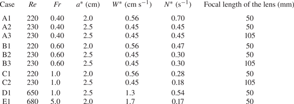
 $Fr$ are comparable to those investigated in this study (cf. tables 1 and 2).
The list of experimental conditions. Two lenses of different focal length (50 mm and 105 mm) are used to observe areas of different size.

The list of parameters used for the numerical simulation. The right two columns show the estimated thickness of the scalar boundary layer of salinity ( $Sc_S$) and fluorescent dye (
 $Sc_C$).

In recent years, many numerical simulations have been performed to investigate this type of flow. The flow around a vertically moving sphere in salt-stratified fluid was simulated with both internal waves and the buoyant jet (Torres et al. Reference Torres, Hanazaki, Ochoa, Castillo and Van Woert2000; Hanazaki, Kashimoto & Okamura Reference Hanazaki, Kashimoto and Okamura2009a; Doostmohammadi, Dabiri & Ardekani Reference Doostmohammadi, Dabiri and Ardekani2014; Zhang, Mercier & Magnaudet Reference Zhang, Mercier and Magnaudet2019), and significant increase of drag by stratification was found. The drag increased up to approximately thirty times that in a homogeneous fluid. The effect of the Schmidt number was then investigated (Hanazaki, Konishi & Okamura Reference Hanazaki, Konishi and Okamura2009b), and it is found that the higher Schmidt number leads to a thinner and faster jet. The density distribution in the salinity boundary layer around the sphere and in the jet was investigated in a more recent and accurate numerical simulation (Hanazaki, Nakamura & Yoshikawa Reference Hanazaki, Nakamura and Yoshikawa2015), and the results show that the Froude number, Schmidt number and Reynolds number contribute in combination to the determination of the thickness of the salinity boundary layer and the radius of the corresponding jet. Theories for a low Reynolds number flow around a small particle have also been developed, although the jet becomes weaker or vanishes at low Reynolds numbers (Camassa et al. Reference Camassa, Falcon, Lin, McLaughlin and Parker2009, Reference Camassa, Falcon, Lin, McLaughlin and Mykins2010; Mehaddi, Candelier & Mehlig Reference Mehaddi, Candelier and Mehlig2018; Lee, Fouxon & Lee Reference Lee, Fouxon and Lee2019).
While the velocity and density distributions have been simulated by numerical simulations, most of the experiments do not measure those values. The vertical movement of a spherical particle has been measured to estimate the drag (e.g. Abaid et al. Reference Abaid, Adalsteinsson, Agyapong and McLaughlin2004; Yick et al. Reference Yick, Torres, Peacock and Stocker2009, and recent studies observe falling disks with a change of orientation (Mrokowska Reference Mrokowska2018; Mercier et al. Reference Mercier, Wang, Péméja, Ern and Ardekani2020). However, the velocity and density distributions in those flows have rarely been measured. The velocity around a sphere was measured by particle image velocimetry (PIV) in several papers (e.g. Hanazaki et al. Reference Hanazaki, Kashimoto and Okamura2009a; Okino, Akiyama & Hanazaki Reference Okino, Akiyama and Hanazaki2017; Akiyama et al. Reference Akiyama, Waki, Okino and Hanazaki2019), but the distribution of salinity or density has not yet been measured.
The initial unsteady process before the steady flow is developed near the obstacle is also of interest, since there is a time lag before the stratification becomes effective. For example, in stratified turbulence, the necessary time lag for the development of kinetic energy or potential energy is of the order of the buoyancy time  $1/N^{*}$. However, the effect of time lag in the present system has not been investigated, while it may significantly affect the initial formation process of the rear vortex and the jet.
In this study, we measure the salinity and hence the density distribution around the sphere by laser-induced fluorescence (LIF), using the approximate proportionality between the salinity and the fluorescent-dye concentration (§ 2.1). The results are compared with numerical simulations which will supplement the experimental results (§ 2.2). We first investigate the density distributions in steady state, including those in the salinity boundary layer and in the jet (§ 3.1). Next, the initial process of jet formation is investigated by LIF and PIV (§ 3.2).
The density distribution measured in the real fluid confirms the predictions by numerical simulations, and improves our understanding of the generation process and the final structure of buoyant jets, including their dependence on the Froude number. For lower  $Fr$, the density boundary layer on the sphere's surface becomes thinner, and the jet downstream of the sphere also becomes thinner, explaining the generation of a faster jet which leads to the reduction of pressure and the increase of drag. When the stratification is moderate (
 $Fr=O(10$)) and the Reynolds number is also moderate (
 $Re=O(10^{2}$)), a rear axisymmetric vortex develops initially, but shrinks as the stratification suppresses the generation of the vortex. On the other hand, under strong stratification (
 $Fr \lesssim 1$), the vortex does not develop even temporarily since the suppression by strong stratification becomes effective in a short time.
2. Methods
2.1. Experimental methods
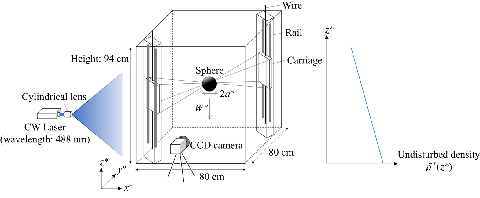
In the present experiment, linearly stratified salt water was generated by a two-tank method (figure 1, cf. Fortuin Reference Fortuin1960), and the velocity fluctuation was minimised by using a non-pulsating metering pump (Smoothflow Pump BPL-10-VTCF-FWS, TACMINA) (Okino et al. Reference Okino, Akiyama and Hanazaki2017). The constant vertical density gradient was verified by sampling a small amount of fluid from the cocks attached to one of the sidewalls of the tank, and density was measured by a density meter (DMA 4500M, Anton Paar) with an accuracy of  $5 \times 10^{-5}$ g cm
 $^{-3}$. Some examples of the initial vertical density distribution are given in Hanazaki et al. (Reference Hanazaki, Kashimoto and Okamura2009a).
A schematic figure of the experimental facilities for LIF. The coordinates move downward with the sphere at a constant speed of  $W^{*}$, with their origin located at the centre of the sphere. The horizontal coordinate
 $x^{*}$ is in the direction of the laser light, and
 $z^{*}$ is the vertical coordinate.

A sphere of radius  $a^{*}=2.0$ or
 $2.5$ cm is used for the experiment. It is made of acrylic, painted in black to reduce the reflection of light, and is supported by eight stainless steel wires whose diameters are 0.1 mm or 0.2 mm. The wires span obliquely across the test tank, with their ends being connected to two rectangular carriage plates which move vertically along the rail (figure 1). There are two vertical rails at the opposite corners of the tank, and a carriage on each rail is driven by a DC motor at a constant speed
 $W^{*}$.
In this study, the salinity, and hence the density, is calculated from the concentration of a fluorescent dye measured by LIF. The transport equations for salinity  $S^{*}$ and dye concentration
 $C^{*}$ are given by
 \begin{equation} \frac{\partial S^{*}}{\partial t^{*}}+ \boldsymbol{u}^{*} \boldsymbol{\cdot} \boldsymbol{\nabla}^{*} S^{*}=\kappa^{*}_{S} {\nabla^{*}}^{2} S^{*}, \end{equation}
and
 \begin{equation} \frac{\partial C^{*}}{\partial t^{*}}+ \boldsymbol{u}^{*} \boldsymbol{\cdot} \boldsymbol{\nabla}^{*} C^{*}=\kappa^{*}_{C} {\nabla^{*}}^{2} C^{*}, \end{equation}
where  $\boldsymbol{u}^*$ is the velocity,
 $\kappa ^{*}_{S}$ and
 $\kappa ^{*}_{C}$ are the diffusion coefficients of salinity and dye, respectively.
When the length is non-dimensionalised by the diameter of the sphere  $2a^{*}$ and velocity by the vertical velocity of the sphere
 $W^{*}$, these equations become
 \begin{equation} \frac{\partial S}{\partial t} + \boldsymbol{u}\boldsymbol{\cdot} \boldsymbol{\nabla} S=\frac{1}{Re Sc_S}\nabla^{2} S \end{equation}
and
 \begin{equation} \frac{\partial C}{\partial t} + \boldsymbol{u}\boldsymbol{\cdot} \boldsymbol{\nabla} C=\frac{1}{Re Sc_C}\nabla^{2} C, \end{equation}
where  $Re=2W^{*} a^{*}/\nu ^{*}$ is the Reynolds number, and
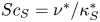 $Sc_S=\nu ^{*}/\kappa ^{*}_S$ and
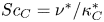 $Sc_C=\nu ^{*}/\kappa ^{*}_C$ are the Schmidt numbers of salinity and fluorescent dye, respectively.
Since (2.3) and (2.4) have the same form except for the diffusion term, approximate proportionality between  $S$ and
 $C$ holds everywhere at any time if the initial distribution satisfies
 $S=\gamma C$ (
 $\gamma =$ constant) everywhere. In the present experiment, the fluorescent dye is initially put into one of the two tanks, and is well mixed before the fluid is pumped up into the test tank. Then, if the dye is initially put into the tank of saltwater, the salinity and dye concentration are proportional in the test tank.
We note, however, that the proportionality becomes incomplete after the fluid flows through the region where  $\nabla ^{2} S$ or
 $\nabla ^{2} C$ is not negligible, since
 $Sc_S$ and
 $Sc_C$ are almost inevitably different. In this study, Rhodamine 110 is used as the fluorescent dye whose Schmidt number should be comparable to Rhodamine B and 6G. According to the literature, the Schmidt number is
 $Sc_C=600$–
 $1200$ (Troy & Koseff Reference Troy and Koseff2005) or even higher (
 $Sc_C=2000$–
 $3000$, Hanson, Davis & Bardeen Reference Hanson, Davis and Bardeen2007), while the Schmidt number of salt is approximately
 $Sc_S=700$. Therefore, while an overall proportionality between
 $C$ and
 $S$ is expected, deviation from proportionality would exist in the scalar boundary layer around the sphere and in the rear jet where the local variation of
 $S$ and
 $C$ is large.
In the present experiment, a continuous-wave laser (488 nm, 4 W) is used. The peak absorption wavelength of Rhodamine 110 ( ${\sim }496$ nm) is near the laser emission wavelength, and its peak fluorescence wavelength is 520 nm. The fluorescence of Rhodamine 110 was measured by a CCD camera with
 $2048 \times 2048$ pixel (Hisense 4MC, Dantec Dynamics; C9300-024, Hamamatsu Photonics; 12 bits, 11 Hz). A band-pass filter with a transmission wavelength of
 $534.5\pm 21.5$ nm is used, which transmits the fluorescence between 513 and 556 nm, while it blocks the direct laser light of 488 nm. The Rhodamine 110 has a high quantum yield
 $(\phi =0.85)$ and a weak dependence on temperature variation (
 ${\sim }0.13\,\%$ K
 $^{-1}$). The insensitivity to temperature is preferable, although the temperatures of the room and the fluid are both kept near
 $20\,^{\circ }\mathrm {C}$ throughout the experiment.
When we need a large observation area to investigate a jet which extends to 25 cm above the sphere, a lens of short focal length (Nikkor 50 mm f/1.2, Nikon) is used to realise a large angle of view. The CCD camera is then placed generally at a long distance ( ${\gtrsim }45$ cm) from the sidewall of the test tank.
On the other hand, when we observe a thin density boundary layer around the sphere, we need to observe a small area with high resolution. Then, we use a larger sphere ( $a^{*}=2.5$ cm) and also a lens of long focal length with a small angle of view (AI Micro-Nikkor 105 mm f/2.8S, Nikon). The CCD camera is then located at approximately 10 cm from the sidewall of the test tank.
The parameters used for the experiments are listed in table 1. We have examined the Froude number ( $Fr=W^{*} /(N^{*} a^{*}$)) dependence of the density field, using the results for cases A1–C2 (
 $Re \sim 220$ and
 $0.40 \le Fr \le 1.0$), or cases D1 and E1 (
 $Re \sim 650$,
 $Fr=1.0$ and 5.0). For all these cases, the previous experiments (figure 4a of Hanazaki et al. Reference Hanazaki, Kashimoto and Okamura2009a) have shown that the flow around the sphere is highly axisymmetric and the direct comparison with the axisymmetric numerical simulation is possible. By comparing case D1 with case E1, we investigate how the initial appearance and disappearance processes of the rear vortex varies with
 $Fr$. In case E1, we investigate the combined effects of larger
 $Fr$ and
 $Re$, which will temporarily produce a larger rear vortex before the stratification becomes effective.
The thickness of the density boundary layer can be estimated by 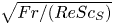 $\sqrt {Fr/(ReSc_S)}$ times the sphere diameter (Hanazaki et al. Reference Hanazaki, Nakamura and Yoshikawa2015), and the observed data are actually consistent with this prediction, as will be shown in figure 4. This means that, when
 $Re=200$,
 $Sc_S=700$ and
 $Fr=0.4$ for example, the scale smaller than
 $\sqrt {Fr/(ReSc_S)} \sim 1/600$ times the sphere diameter must be resolved. This could be achieved only by the lens of long focal length.
In the LIF method, the relation between the radiation energy of the fluorescent light from a unit volume  $E^{*}$ and the dye concentration
 $C^{*}$ is given by
 \begin{equation} E^{*}=E_{0}^{*} C^{*} \phi \varepsilon^{*} \exp (-\varepsilon^{*} l^{*} C^{*}), \end{equation}
where  $E_{0}^{*}$ is the incident energy of light at the wall of the test tank,
 $\phi$ is the quantum yield,
 $\varepsilon ^{*}$ is extinction coefficient and
 $l^{*}$ is the length of the light path.
The value of  $E^{*}$ is usually assumed to be proportional to the dye concentration
 $C^{*}$. As can be inferred from (2.5), the proportionality is realised when the dye concentration is small enough to satisfy
 $\exp (-\varepsilon ^{*} l^{*} C^{*}) \approx 1$. However, as the concentration becomes larger, the proportionality becomes imperfect. In the present experiment, where there is a large spatial difference in concentration, a modified method which allows deviation from proportionality is preferable.
The intensity of fluorescent light  $I^{*}$ with the background noise of the CCD camera
 $I_{back}^{*}$ is given by
 \begin{equation} I^{*} = I_{back}^{*} +\beta E_{0}^{*} C^{*} \phi \varepsilon^{*} \exp(-\varepsilon^{*} l^{*} C^{*}), \end{equation}
where  $\beta$ is the translation rate. This can be approximated under the condition of
 $\varepsilon ^{*} l^{*} C^{*} \ll 1$ by a second-order function of
 $C^{*}$
 \begin{equation} I^{*} \simeq I_{back}^{*} + \beta E_{0}^{*} C^{*} \phi \varepsilon^{*} (1-\varepsilon^{*} l^{*} C^{*}). \end{equation}
Therefore, in the calibration for the present experiment, it would be appropriate to assume a parabolic relation
 \begin{equation} I^{*} = a_{0}^{*} C^{* 2} + a_{1}^{*} C^{*} + a_{2}^{*}, \end{equation}
and to measure the value of  $I^{*}$ for systematically changed values of
 $C^{*}$. Then, we determine the values of the coefficients
 $a_{0}^{*}$,
 $a_{1}^{*}$ and
 $a_{2}^{*}$ by the least squares method. Once the function (2.8) is determined by calibration, we can use it to compute the value of
 $C^{*}$ from the measured value of
 $I^{*}$, simply solving the quadratic equation of
 $C^{*}$ (2.8).
When we observe the boundary layer of the sphere (figure 4) or the horizontal cross-section of the jet (figure 5), we have averaged the density perturbation observed at the same point but at ten successive frames, to reduce the effect of the experimental noise in the observed data.
2.2. Numerical methods
In this study, numerical simulations also have been performed for comparison with the experiments. The governing equations are the Navier–Stokes equations under Boussinesq approximation
 \begin{equation} \frac{\partial \boldsymbol{u}}{\partial t}+(\boldsymbol{u}\boldsymbol{\cdot} \boldsymbol{\nabla}) \boldsymbol{u} ={-}\boldsymbol{\nabla} p^{\prime}-\left(\frac{2}{Fr}\right)^{2}\rho^{\prime} \boldsymbol{\hat{z}}+\frac{1}{Re}\nabla^{2}\boldsymbol{u}, \end{equation}
the mass-conservation equation
 \begin{equation} \boldsymbol{\nabla} \boldsymbol{\cdot} \boldsymbol{u} =0, \end{equation}
and the transport equation for salinity perturbation ( $Sc_S=700$)
 \begin{equation} \frac{\partial S^{\prime}}{\partial t}+ \boldsymbol{u}\boldsymbol{\cdot} \boldsymbol{\nabla} S^{\prime} =w-1+\frac{1}{ReSc_S}\nabla^{2} S^{\prime}, \end{equation}
assuming proportionality between the density and salinity
 \begin{equation} \rho^{\prime}=\beta_{0} S^{\prime}. \end{equation}
Here,  $\boldsymbol {u}$ is the velocity,
 $t$ is the time,
 $p^{\prime }$ is the pressure perturbation,
 $\rho ^{\prime }$ is the density perturbation,
 $S^{\prime }$ is the salinity perturbation and
 $\beta _0$ is the haline contraction coefficient. In the Navier–Stokes equations, the length is scaled by
 $2a^{*}$, the velocity by
 $W^{*}$, the pressure by
 $\rho _0^{*} W^{* 2}$ and the density by
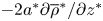 $-2a^{*} \partial \overline {\rho }^{*}/\partial z^{*}$, where
 $\overline {\rho }^{*}(z^{*}, t^{*})$ is the undisturbed density distribution and
 $\rho _0^{*}\, (=\overline {\rho }^{*}(0, 0))$ is the reference density. The term
 $-1$ appears on the right-hand side of (2.11) since the above equations are written in the frame moving downward with the sphere.
The transport equation for a passive scalar, i.e. for a fluorescent dye, is
 \begin{equation} \frac{\partial C^{\prime}}{\partial t}+\boldsymbol{u}\boldsymbol{\cdot} \boldsymbol{\nabla} C^{\prime} =w-1+\frac{1}{ReSc_C}\nabla^{2} C^{\prime}. \end{equation}
We have used a fixed value of  $Sc_S=700$ for salinity, and several sets of Froude number and Reynolds number (table 2) for comparison with the experiments. For case C
 $1'$
 $(Re=220, Fr=1)$ and E
 $1'$ (
 $Re=680, Fr=5$) which correspond to case C1 and E1 in LIF (table 1), the equation for a passive scalar (2.13) is also solved along with (2.9)–(2.12), assuming
 $Sc_C=2000$ for Rhodamine 110.
Comparison between (2.11) and (2.13) shows that the concentration  $C^{\prime }$ is always proportional to
 $\rho ^{\prime }$ everywhere if
 $Sc_C=Sc_S\, (=700)$, provided that their initial distributions are the same. The deviation from the proportionality appears if
 $Sc_C \neq Sc_S$, mainly in the area of significant molecular diffusion.
The numerical method is the same as the previous numerical studies (Torres et al. Reference Torres, Hanazaki, Ochoa, Castillo and Van Woert2000; Hanazaki et al. Reference Hanazaki, Konishi and Okamura2009b, Reference Hanazaki, Nakamura and Yoshikawa2015) which used the finite difference method combined with generalised curvilinear coordinates (Thames et al. Reference Thames, Thompson, Mastin and Walker1977).
In the present numerical simulation, axisymmetry of the flow around the  $z$-axis is assumed. The number of grid points is
 $360 \times 1100$, with 360 points in the direction along the sphere surface and 1100 points in the direction normal to the sphere surface. The grid spacing is much smaller near the sphere surface where there is a thin scalar boundary layer. For example, in case C1
 $^{\prime }$ (
 $Re=220$,
 $Fr=1$,
 $Sc_C=2000$), the thickness of the scalar boundary layer is estimated as
 $\sqrt {Fr/(ReSc_C)} =\sqrt {1/(220 \times 2000)}=1.51 \times 10^{-3}$ (Hanazaki et al. Reference Hanazaki, Nakamura and Yoshikawa2015). The grid used for the present numerical simulation has at least eleven grid points in this estimated thickness, and actually gives sufficient numerical accuracy (cf. Appendix A).
While axisymmetry of the flow is assumed in the present numerical simulation, the flow of a homogeneous fluid past a sphere becomes non-axisymmetric for  $Re\gtrsim 200$ (Taneda Reference Taneda1956). The experiments in this study have been performed for
 $Re \sim 220$ and
 $Re \sim 680$, suggesting the possibility of a non-axisymmetric flow for
 $Re \sim 680$. However, the stratification actually inhibits the development of a large rear vortex which would lead to an asymmetric vortex shedding (figure 4a of Hanazaki et al. Reference Hanazaki, Kashimoto and Okamura2009a), and the inhibition process is also investigated in this study.
The numerical simulation is performed until  $t=10$ for comparison with the experiments. The simulation period is determined by considering the maximum non-dimensional time
 $t_{max}$ realised in the experiments. Since the vertical movable range of the sphere in the test tank is
 $H^{*} \sim 70 \ \textrm {cm}$,
 $t_{max}$ is estimated by
 $t_{max}=W^{*} t_{max}^{*}/(2a^{*})=H^{*}/(2a^{*}) \sim 14$ when the sphere radius is
 $a^{*} =2.5$ cm. This relatively short time development would be another reason for the axisymmetry of the flow in the experiments. Even without stratification and at relatively high Reynolds number, the flow would be axisymmetric for this short period.
We also note that the density distribution on the sphere's surface becomes steady before  $t=10$, if the Froude number is low enough (
 $Fr \lesssim 1$), with
 $Re=200$ and
 $Sc_S=700$ (cf. figure 11 of Hanazaki et al. Reference Hanazaki, Nakamura and Yoshikawa2015). Since the time scale of scalar diffusion is larger for a higher Schmidt number, a longer time is necessary to achieve a steady state for a passive scalar of
 $Sc_C=2000$, and its distribution in the jet becomes steady at
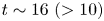 $t \sim 16\ (>10)$ (cf. Appendix B and figure 5). However, the steady state is achieved much earlier at lower heights (figure 13 of Hanazaki et al. Reference Hanazaki, Nakamura and Yoshikawa2015), and the passive-scalar distribution near the equator of the sphere (
 $z=0$) would become steady well before
 $t=10$, even if
 $Sc_C=2000$ (cf. figure 4).
The solutions of (2.11) and (2.13), i.e.  $C^{\prime }$ and
 $S^{\prime }$, or
 $C$ and
 $S$, do not agree when
 $Sc_C$ is not equal to
 $Sc_S\ (=700)$. This occurs in numerical simulations with
 $Sc_C=2000$, and in the corresponding experiments where Rhodamine 110 (
 $Sc_C \sim 2000$) is used as a passive scalar. However, in presenting the results of this study, the value of
 $C$ or
 $C^{\prime }$ is always substituted for the value of
 $\rho\ (=S)$ or
 $\rho ^{\prime }\ (=S^{\prime })$, since we want to know the value of
 $\rho$ or
 $\rho ^{\prime }$ even if it is an approximate value. This point needs to be taken into consideration when we interpret the results.
3. Results
3.1. Density distribution in steady state
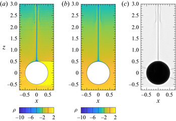
The density distribution in the vertical plane which passes through the centre of the sphere, i.e.  $y=0$, is shown in figure 2 for the case of
 $Fr=0.4$ and
 $Re=220$ (
 $t \simeq 10$). This figure is obtained by three different methods, i.e. by LIF, numerical simulation and shadowgraph, all of which show a thin jet typically observed at low Froude numbers and moderate Reynolds numbers (
 $Fr \lesssim 3$,
 $50 \lesssim Re \lesssim 500$). For this set of parameters, the jet is straight and fully developed near the sphere (
 $z<3$), but becomes unstable and meanders at larger height (
 $z \gtrsim 3$), as observed in figure 3(a). The density distributions obtained by LIF (figure 2a) and numerical simulation (figure 2b) are similar, and the density in the jet is much smaller than the surrounding fluid at the same height, showing that the large buoyancy force is the origin of the jet. Previous numerical simulations have shown that the fluid in the jet was originally in the upper part of the stratified fluid, and was pulled down by the sphere before it goes up in the jet (Hanazaki et al. Reference Hanazaki, Nakamura and Yoshikawa2015). The density distribution observed by LIF confirms this prediction.
Distribution of density  $\rho$ in the vertical plane
 $y=0$ at
 $t \simeq 10$ (
 $Fr=0.40$,
 $Re=220$). (a) LIF (case A1); (b) numerical simulation (A
 $1'$); (c) shadowgraph experiment which would correspond to
 $\nabla ^{2} \rho$ (A1).

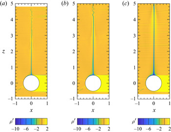
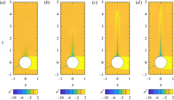
Froude number dependence of the density perturbation  $\rho ^{\prime }$ measured by LIF in the vertical plane (
 $y=0$) at
 $t \simeq 10$ (
 $Re \simeq 220$); (a)
 $Fr=0.40$ (case A1), (b)
 $Fr=0.60$ (B1), (c)
 $Fr=1.0$ (C1).

The result of shadowgraph method (figure 2c), which represents the second derivative of density  $\nabla ^{2} \rho$, includes a bell-shaped structure at the height of
 $2 \lesssim z \lesssim 3$. This structure could be identified also in the LIF and numerical simulation, but the image is more vague, mainly because these two methods observe the density and not its second derivative. The origin of the bell-shaped structure is in the downward velocity due to the internal wave (Hanazaki et al. Reference Hanazaki, Kashimoto and Okamura2009a). Then, the vertical position of the bell-shaped structure is determined by the vertical wavelength of the internal wave. We observe in figure 3 that the structure appears at a higher position as the Froude number increases, in qualitative agreement with a characteristic of the internal wave that the vertical wavelength is proportional to the Froude number (e.g. Torres et al. Reference Torres, Hanazaki, Ochoa, Castillo and Van Woert2000). Since the thin jet generates a strong shear, the jet itself becomes unstable high above the sphere (
 $z \gtrsim 3.5$). The instability has been observed even when the Reynolds number is small (e.g.
 $Re=10$ in Akiyama et al. Reference Akiyama, Waki, Okino and Hanazaki2019), as long as the jet is thin enough.
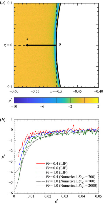
Since the fluid in the jet originates from the boundary layer around the sphere, measurement of density near the sphere surface would be useful to understand the relation between the jet and the boundary layer. The density distribution in the density boundary layer on the  $x$-axis above the equator of the sphere (
 $x=-0.5-d$ with
 $0 < d \leq 0.05$,
 $y=z=0$) is presented in figure 4 for
 $Fr=0.4, 0.6$ and
 $1.0$ (
 $Re \simeq 220$).
Distribution of density perturbation  $\rho ^{\prime }$ on the
 $x$-axis at
 $t \simeq 10$, where
 $d=-x-0.5\ (\leq 0.1)$ is the horizontal distance from the sphere surface located at
 $x=-0.5$ (i.e.
 $d=0$). The results of LIF and numerical simulations on the horizontal line
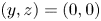 $(y, z)=(0, 0)$ indicated in (a) is plotted in (b). The experimental data in (b) are
 $Fr=0.40$ (A3), 0.60 (B3) and 1.0 (C2). The Schmidt number of the fluorescent dye is
 $Sc_C \simeq 2000$ in LIF, while it is assumed to be either
 $Sc_C=700$ or 2000 in numerical simulations. Other parameters, i.e.
 $Re \simeq 220$ and
 $Sc_S \simeq 700$, are the same in all the cases (cf. table 1). The LIF data are averaged over ten successive frames photographed at 11.3 Hz.

The density perturbation is negative ( $\rho ^{\prime }<0$) everywhere near the sphere surface since the sphere pulls down the upper light fluid. The lower value of
 $\rho ^{\prime }$ near the sphere indicates that the fluid attached to the sphere originates from a higher region.
In both LIF and numerical simulations, the value of  $\rho ^{\prime }$ near the sphere is more negative for higher
 $Fr$, showing that the sphere drags the fluid for a longer distance. This confirms the results of previous numerical simulations (Hanazaki et al. Reference Hanazaki, Nakamura and Yoshikawa2015) that an obstacle vertically drags the fluid in the boundary layer for a longer distance when the Froude number is higher.
The perturbation quickly approaches zero away from the sphere's surface ( $d \gtrsim 0.02$) since the density boundary layer is very thin. If we fit the numerical result for
 $d \gtrsim 0.02$ by an exponential function in the form of
 $\rho ^{\prime } \propto \exp (-d/\lambda )$ (
 $\lambda$: length scale of the scalar boundary layer),
 $\lambda \sim 9.5 \times 10^{-3}$ for
 $Fr=0.4$, while
 $\lambda \sim 2.0 \times 10^{-2}$ for
 $Fr=1.0$. This means that the returning to
 $\rho ^{\prime }=0$ occurs over a longer distance for a larger
 $Fr$, consistent with a thicker scalar boundary layer.
The dimensional analysis, which assumes that the length scale is written only by  $\kappa _S^{*}$ and
 $N^{*}$, gives the fundamental scale of stratified fluids (Hanazaki et al. Reference Hanazaki, Nakamura and Yoshikawa2015)
 \begin{equation} l^{*}_{\kappa}=\sqrt{\frac{\kappa_S^{*}}{N^{*}}}, \end{equation}
which can be rewritten in non-dimensional form as
 \begin{equation} l^{*}_{\kappa}/2a^{*}=\left( \frac{Fr}{2ReSc_S} \right)^{1/2}. \end{equation}
Previous numerical simulations have shown that this gives a good estimation for the half width at half maximum (HWHM) of the distribution of  $\nabla ^{2} \rho ^{\prime }/ReSc_S$ across the jet. The proportionality to
 $Fr^{1/2}$ and
 $Re^{-1/2}$ has been actually observed in numerical simulations (figures 19a and 20a of Hanazaki et al. Reference Hanazaki, Nakamura and Yoshikawa2015), and (3.2) gives approximately 1.5 times the value obtained by the numerical simulation. The proportionality to
 $Sc_S^{-1/2}$ has also been confirmed for
 $0.7 \lesssim Sc_S \lesssim 700$ (authors’ unpublished observations).
The thickness of the density boundary layer is difficult to define, but the distance of the point of minimum  $\nabla ^{2} \rho ^{\prime }/ReSc_S$ from the equator of the sphere is approximately four times the estimation given by (3.2). When
 $Fr=1$,
 $Re=200$ and
 $Sc_S=700$, the relation (3.2) gives
 $2 \times 10^{-3}$, while the simulation result shows that the HWHM of the jet is
 $1.2 \times 10^{-3}$ (cf. figure 19a of Hanazaki et al. Reference Hanazaki, Nakamura and Yoshikawa2015), and the distance of the minimum
 $\nabla ^{2} \rho ^{\prime }/ReSc_S$ from the equator of the sphere is approximately
 $d=8 \times 10^{-3}$ (cf. figure 21 of Hanazaki et al. Reference Hanazaki, Nakamura and Yoshikawa2015). This is verified by the LIF data given in figure 4.
Numerical result for  $Sc_C=2000$ (
 $Sc_S=700$,
 $Fr=1.0$) gives lower value of
 $\rho ^{\prime }$ near the sphere surface than the result for
 $Sc_C=700$, and gives better agreement with the experiment. This is because we observe in LIF the fluorescent dye (Rhodamine 110) whose Schmidt number is
 $Sc_C \sim 2000$, and not the salt (
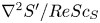
 $Sc_C=Sc_S=700$). The difference between (2.3) and (2.4), or (2.11) and (2.13), becomes apparent only where the diffusion terms
 $\nabla ^{2} S^{\prime }/ReSc_S$ and
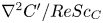 $\nabla ^{2} C^{\prime }/ReSc_C$ become large, i.e. in the scalar boundary layer or in the jet. The minimum value of
 $\rho ^{\prime }$ in figure 4 is smaller for
 $Sc_C=2000$ since the diffusion is weak and the scalar concentration is better conserved along the motion of the fluid. The thickness of the density boundary layer and the radius of the jet estimated for salt
 $(Sc_C=700)$ would be
 $\sqrt {2000/700}=1.7$ times of those estimated for dye
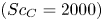 $(Sc_C=2000)$. We should note the difficulty in calculating the value of
 $\nabla ^{2} \rho ^{\prime }/ReSc_S$ from the data of LIF, since the small noise in
 $\rho ^{\prime }$ leads to large fluctuations in the second-order derivative. Therefore, we show only the data of
 $\rho ^{\prime }$ in this paper.
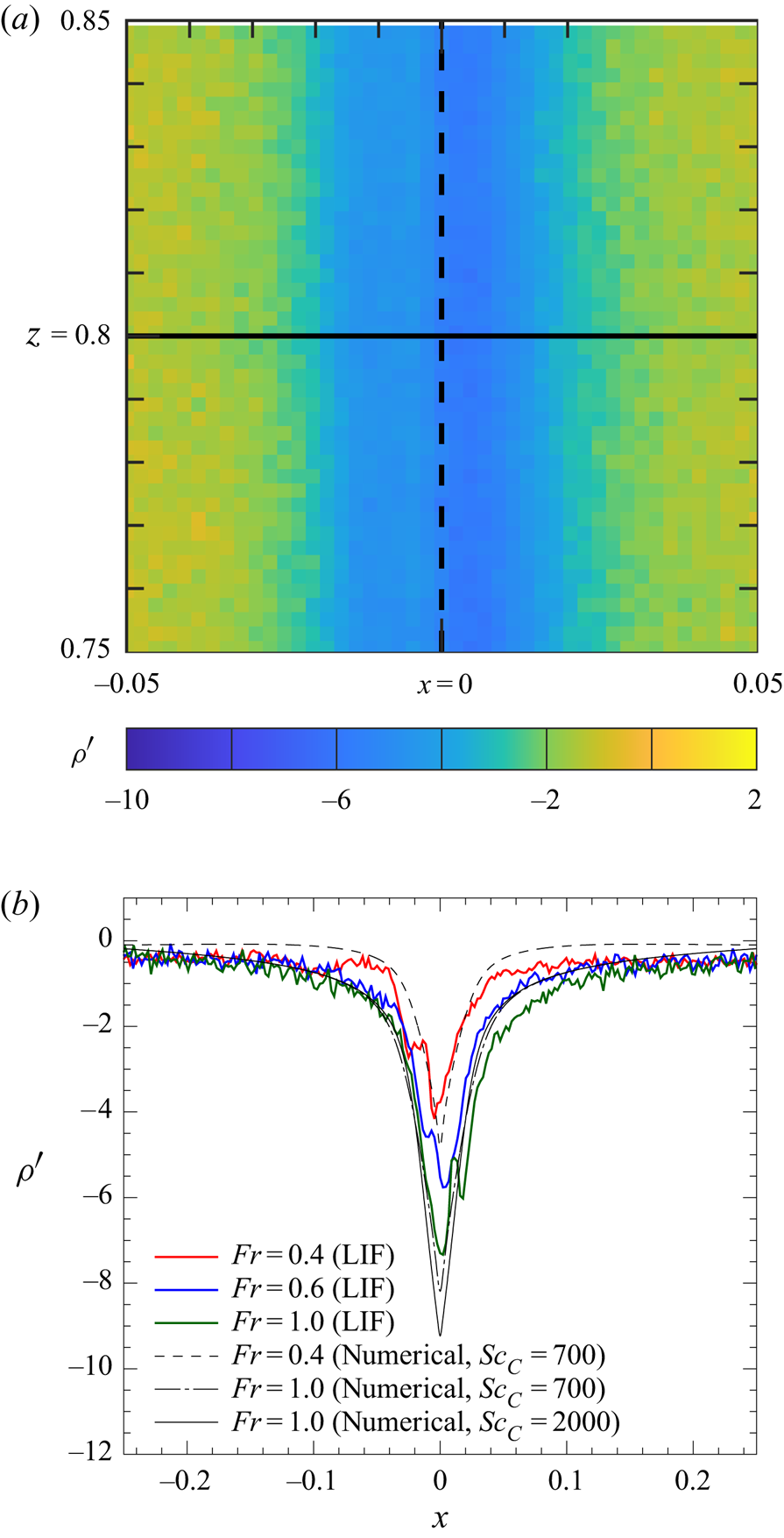
We next investigate the internal structure of the jet. Distribution of density perturbation  $\rho ^{\prime }$ on a horizontal line parallel to the
 $x$-axis (
 $y=0$ and
 $z=0.8$) is shown in figure 5. The line is 0.3 above the rear/upper stagnation point (
 $z=0.5$) of the sphere. The density perturbation is more significantly negative for larger
 $Fr$, as observed in the scalar boundary layer (figure 4), since the sphere drags the fluid for a longer length. Previous numerical results for
 $Sc_S=700$ (figure 11 of Hanazaki et al. Reference Hanazaki, Nakamura and Yoshikawa2015) also show that the density perturbation at the upper stagnation point of the sphere (i.e.
 $z=0.5$ and
 $x=y=0$) becomes more negative for larger
 $Fr$ in the final steady state. The jet becomes broader as the Froude number increases according to (3.2), corresponding to the thicker density boundary layer on the sphere surface.
Distribution of the density perturbation  $\rho ^{\prime }$ on a horizontal line across the vertical jet (b). The data on the horizontal line
 $(y, z)=(0, 0.8)$, located above the stagnation point of the sphere
 $(x, y, z)=(0, 0, 0.5)$ and indicated in (a), is presented in (b). The parameter values are the same as figure 4, but cases A2, B2 and C1 are used.

The negative peaks of  $\rho ^{\prime }$ at
 $x=0$ (i.e. on the
 $z$-axis) obtained by the experiments are generally lower than the numerical simulations for the same
 $Fr\ (=0.4 \ \textrm {and} \ 1.0)$. There are two possible reasons for this difference, and they are discussed in detail in Appendix C, but important points are outlined here.
One is the non-zero thickness of the laser light sheet ( $D_L \neq 0$). Since the laser light sheet has a non-zero thickness, the CCD camera observes the fluorescence from the whole region across the light sheet. On the other hand, the distribution of fluorescent scalar or density is not uniform across the sheet. Then, the CCD camera observes the average value of fluorescence across the light sheet. The actual value of
 $D_L$ in the present LIF is measured in a homogeneous fluid, and it is approximately 0.015 (if the dimensional value
 $D_L^{*}=0.6$ mm is scaled by the sphere diameter
 $2a^{*}=4$ cm). Since the diameter of the jet
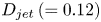 $D_{jet}\,(=0.12)$ is much larger than
 $D_L$, the measurement error due to
 $D_L (\neq 0)$ is not significant. The maximum error appears in the peak value of
 $\rho ^{\prime }$ (or
 $C^{\prime }$) at the centre of the jet (
 $x=0$), but is limited to 6.8 % in case C
 $1'$. The other reason is the small lateral displacement (
 $y_L$) of the light sheet from
 $y=0$. This second reason causes errors larger than the first reason. For example, when
 $y_L =D_L/2$, the maximum reduction in the peak value is 12.8 % in case C
 $1'$. Combined with the first reason, the total reduction is approximately 20 %. This estimation is comparable to the difference between the numerical simulation and LIF, suggesting that
 $y_L =D_L/2$ is close to the actual value. The error is maximum at
 $x=0$, but decreases rather rapidly as
 $|x|$ increases. For example, the error is less than 10 % for
 $|x|>0.056D_{jet}$, and is less than 5 % for
 $|x|>0.2D_{jet}$, showing that the large error is limited to the very central region of the jet.
It should be noted that the measurement error due to  $D_L \neq 0$ and
 $y_L \neq 0$ is negligibly small when we observe the scalar boundary layer on the equator of the sphere as in figure 4, since both
 $D_L$ and
 $y_L$ are significantly smaller than the sphere diameter (
 $=1$).
Finally, we should also note that the above error estimation assumed the most typical value of 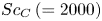 $Sc_C\,(=2000)$. The measurement of the diffusion coefficient is a subtle problem, and the value often varies among the literature in chemistry. In the case of Rhodamine,
 $Sc_C=600$ is the lowest value in the literature. Then, if
 $Sc_C=700$ for example, the peak value of
 $|\rho '|$ is approximately 10 % lower in the numerical simulation (figure 5), and the maximum error in LIF reduces to approximately 10 %.
3.2. Initial process of jet formation
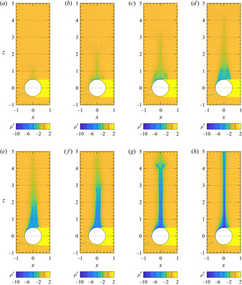
To investigate the generation process of a jet, the initial development of the density distribution for  $(Fr, Re)=(5.0, 680)$ is shown in figure 6. While the isopycnals generally do not agree with the streamlines in unsteady flow, they still represent the particle paths if the molecular diffusion of salinity is negligible or
 ${\rm D}S/{\rm D}t=0$ (cf. (2.3)) is satisfied. This conservation relation would be satisfied except for the thin salinity boundary layer around the sphere, where the effect of molecular diffusion is significant.
Generation process of a jet observed by LIF for case E1 ( $Fr \simeq 5.0$,
 $Re \simeq 680$); (a)
 $t \simeq 1$, (b)
 $t \simeq 2$, (c)
 $t \simeq 3$, (d)
 $t\simeq 4$, (e)
 $t\simeq 5$, (f)
 $t \simeq 6$, (g)
 $t \simeq 7$ and (h)
 $t \simeq 8$.

Larger  $Fr$ and
 $Re$ are selected here since the downstream separated vortex is larger for a weaker stratification and a higher Reynolds number, and the effect of stratification can be identified more clearly. As expected, a broad wake with a large axisymmetric vortex develops initially (
 $t \lesssim 4$), as if it were in a homogeneous fluid. The Reynolds number used here is higher than the threshold value to support an axisymmetric flow (
 $Re \simeq 200$, e.g. Taneda Reference Taneda1956), but we know that the separated vortex remains axisymmetric until non-axisymmetric instability develops, even at a high Reynolds number. While the axisymmetry of the flow for
 $t \lesssim 4$ is mainly due to the short developing time, the effect of stratification would exist already in this initial period. In general, it takes a buoyancy time of order
 $t^{*} \sim 1/N^{*}$ (i.e.
 $t=W^{*}t^{*}/2a^{*} \sim Fr/2$) before the stratification becomes effective, and the value is 2.45 in the present case, so that the stratification should have some effects before
 $t=4$. Indeed, a close examination of the velocity field reveals later (figures 9 and 10) that the stratification comes into effect before
 $t=3$ to reduce the size of the separated vortex. Namely, the stratification becomes effective before the instability due to high Reynolds number appears.
After the stratification effects become conspicuous at  $t \sim 3$, the vortex-like recirculating region in the density distribution (figure 6) shrinks horizontally, while it elongates vertically. Then, a vertically long structure of low density appears along the
 $z$-axis. Comparison with the velocity distribution shows that this actually corresponds to the development of a jet. The vertical velocity on the
 $z$-axis is zero at the upper end of the axisymmetric vortex, becomes positive (
 $w>0$) above that point and increases further with height to become positive even in the laboratory frame (
 $w>1$), constituting a buoyant jet (cf. figure 9). The upper end of the low-density region, or the jet, is at
 $z \simeq t$, which is the initial height of the sphere. This can be confirmed for
 $t \leq 4$ (figure 6a–d), and shows that the fluid dragged by the sphere returns to its original height if the salinity, and hence the density, is not altered by the molecular diffusion. As already noted, the molecular diffusion is negligible outside the salinity boundary layer around the sphere. In the density distribution, the elongated structure would finally correspond to the jet for
 $t \gtrsim 6$.
We have performed also a numerical simulation for case E $1'$
 $(Fr=5,$
 $Re=680,$
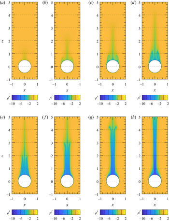
 $Sc_C=2000)$, and compared the results with the experiments (case E1). The density distribution obtained by the simulation with
 $Sc_C=2000$ (figure 7) agrees well with the experiment in the overall structure of the wake and jet. The agreement is owed partly to the axisymmetry of the flow even at
 $Re=680\, (>200)$, due to the short period of time and stratification. However, the jet observed in the experiment is a little thinner than that in the numerical simulation. One possible reason for this difference is the somewhat incomplete axisymmetry of the flow and the subsequent weaker rear vortex in the experiment. This can be identified by the smaller number of streamlines in the rear vortex of the experiment (cf. figures 9 and 10). Then, the vortex disappears and the jet becomes thin in a shorter time.
Generation process of a jet obtained by numerical simulation for case E $1'$ (
 $Fr=5$,
 $Re=680$,
 $Sc_C=2000$); (a)
 $t=1$, (b)
 $t=2$, (c)
 $t=3$, (d)
 $t=4$, (e)
 $t=5$, (f)
 $t=6$, (g)
 $t=7$ and (h)
 $t=8$.

To investigate exclusively the effect of stratification, the development of the density distribution at a stronger stratification ( $Fr=1.0$), but with approximately the same Reynolds number (
 $Re=650$), is measured by LIF (figure 8). The jet-like structure appears and extends upward also in this case, but an axisymmetric separated vortex does not appear, since the Froude number is smaller and the stronger stratification inhibits the generation of the vortex. If we consider this case in terms of the time scale, the buoyancy time is much shorter (
 $t=W^{*}t^{*}/2a^{*} \sim Fr/2 =0.5$), and the stratification effect becomes significant in a short time, well before the vortex is generated.
Generation process of a jet observed by LIF (D1) at  $Fr \simeq 1.0$ and
 $Re \simeq 650$; (a)
 $t \simeq 1$, (b)
 $t \simeq 2$, (c)
 $t \simeq 3$ and (d)
 $t \simeq 4$.

The jet ceases its vertical extension at  $t \sim 4$ (figure 8d) in this case (
 $Fr=1.0$), while the extension continues even after
 $t=8$ for larger
 $Fr(=5.0$, figure 6h). The difference reflects the fact that the sphere drags the fluid vertically only for a short distance under strong stratification, and the time necessary for establishing a steady state is shorter. Previous numerical simulations have shown that the non-dimensional duration time of density conservation at the rear stagnation point of the sphere (
 $t_{c}=W^{*}t^{*}_{c}/2a^{*}$) is comparable to the non-dimensional dragged length of the upper fluid by the sphere (Hanazaki et al. Reference Hanazaki, Nakamura and Yoshikawa2015). For example, numerical simulations at
 $Re=200$ show that
 $t_{c} \simeq 6$ for
 $Fr=1$, while
 $t_{c} \simeq 17$ for
 $Fr=5$ (cf. figure 12a of Hanazaki et al. Reference Hanazaki, Nakamura and Yoshikawa2015). This leads to the difference in the length of the jet-like structure presented in figures 6 and 8.
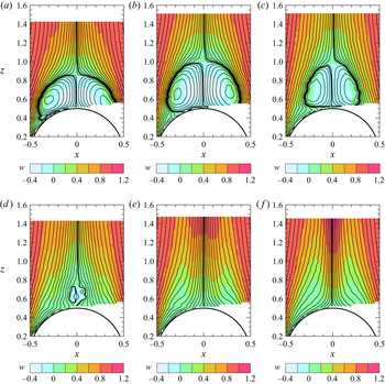
We finally consider the velocity distribution in the near wake of a sphere to investigate the effect of stratification on the rear vortex. The streamlines and the distribution of vertical velocity is shown in figure 9 for parameters that are the same as figures 6 and 7  $(Fr=5.0, Re=680)$. The horizontal and vertical velocity (
 $u, w$) in the vertical plane is measured by PIV using the same facility and method as Okino et al. (Reference Okino, Akiyama and Hanazaki2017), and the Stokes’ streamfunction is calculated by integrating the velocity in the vertical plane, ignoring the small azimuthal velocity around the
 $z$-axis. Then, the contours of Stokes’ streamfunction are drawn as the streamlines. The results show that a vortex ring develops initially and becomes larger until
 $t \sim 3$ (figure 9b). However, it shrinks first horizontally (
 $3 \leq t \leq 4$, figure 9b,c), then also vertically (
 $4 \leq t \leq 5$, figure 9c,d) before it completely disappears at
 $t \simeq 6$ (figure 9e). The process corresponds to the development of the density distribution observed by LIF (cf. figure 6).
Formation process of the jet observed by PIV at the largest Froude number ( $Fr=5.0$) and the largest Reynolds number of
 $Re \simeq 680$. Stokes’ streamlines are drawn for
 $\psi =\pm n^{4}\times 10^{-6}\; (n=0,\, 1,\, 2,\,\ldots )$; (a)
 $t \simeq 2$, (b)
 $t \simeq 3$, (c)
 $t \simeq 4$, (d)
 $t \simeq 5$, (e)
 $t \simeq 6$ and (f)
 $t\simeq 7$.

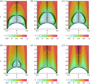
It is of interest to note that the separation point on the sphere moves rearward from the early time, even when the vortex ring is still developing ( $2 \leq t \leq 3$). Namely, the vortex shrinks horizontally whereas it develops vertically. This process can be more clearly observed in the results of numerical simulation (figure 10). After the separation point reaches the rear stagnation point of the sphere, the vortex is detached from the sphere at
 $t=5$ (figure 10d), and finally disappears at
 $t=6$. It is important to note that the appearance and disappearance of the vortex ring is an initial transient phenomenon, and the vortex never appears again after a steady flow is established without a vortex.
Formation process of the jet observed by numerical simulation at the largest Froude number ( $Fr=5$) and the largest Reynolds number of
 $Re=680$; (a)
 $t=2$, (b)
 $t=3$, (c)
 $t=4$, (d)
 $t=5$, (e)
 $t=6$, and (f)
 $t=7$.

4. Conclusion
In this study, the density distribution in the flow generated by a sphere descending in salt-stratified fluid was measured by LIF, assuming approximate proportionality between the salinity and the concentration of a fluorescent dye. The density distributions in steady state and in the initial development are both measured.
In steady flow, flows under strong stratification ( $0.4 \leq Fr \leq 1.0$) are considered. The overall patterns of the buoyant jet are demonstrated first, and the density distributions in the thin salinity boundary layer of the sphere, and those across the thin jet, are measured. The effect of Schmidt number is also considered in the region where the molecular diffusion of salinity and dye is significant. The salinity boundary layer and the jet become thinner for a smaller Froude number, in agreement with the numerical simulations. The agreement is good, especially when the actual Schmidt number of the passive dye (
 $Sc=2000$) is used for the computation, confirming the accuracy of the LIF measurement.
In the initial development of the flow, results for a weaker stratification ( $Fr=5.0$) and a larger Reynolds number (
 $Re=680$) show the development of a vortex-like structure which extends vertically while shrinking horizontally. The corresponding velocity distribution obtained by PIV and numerical simulation indeed shows the initial transient development of a rear vortex. The vortex initially grows but shrinks, first horizontally, then vertically, and becomes a small detached vortex after the separation point reaches the rear stagnation point of the sphere. The detached vortex then disappears in a short time. These processes occur since it takes approximately a buoyancy time (
 ${\sim }1/N^{*}$) before the stratification becomes effective. After its disappearance, the vortex never appears again since the stratification is effective continuously.
Funding
This study was supported by JSPS KAKENHI grant nos. 24656124, 15K17972. Computational resources were provided by Tohoku University through the HPCI System Research Project (hp200020) and by the Earth Simulator Center of Japan Agency of Marine-Earth Science and Technology.
Declaration of interests
The authors report no conflict of interest.
Appendix A. Effects of grid resolution on the numerical solutions
The effects of grid resolution have been examined in the previous study for  $Sc=700$ with
 $Re=200$ and
 $Fr=0.3$ (Hanazaki et al. Reference Hanazaki, Nakamura and Yoshikawa2015). The minimum estimated thickness of the scalar boundary layer in this study (
 $\sqrt {Fr/(ReSc_{C})}=1.51 \times 10^{-3}$, cf. case C
 $1'$ in table 2) is close to, and even larger than, the previous study (
 $\sqrt {Fr/(ReSc)}=1.46 \times 10^{-3}$), but the passive scalar in this study has a higher Schmidt number (
 $Sc_C=2000$, i.e. cases C
 $1'$ and E
 $1'$ in table 2). Then, we examine here the effects of grid resolution on the results for case C
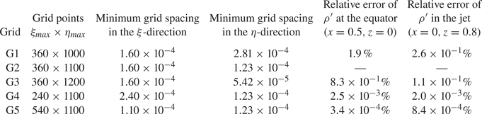
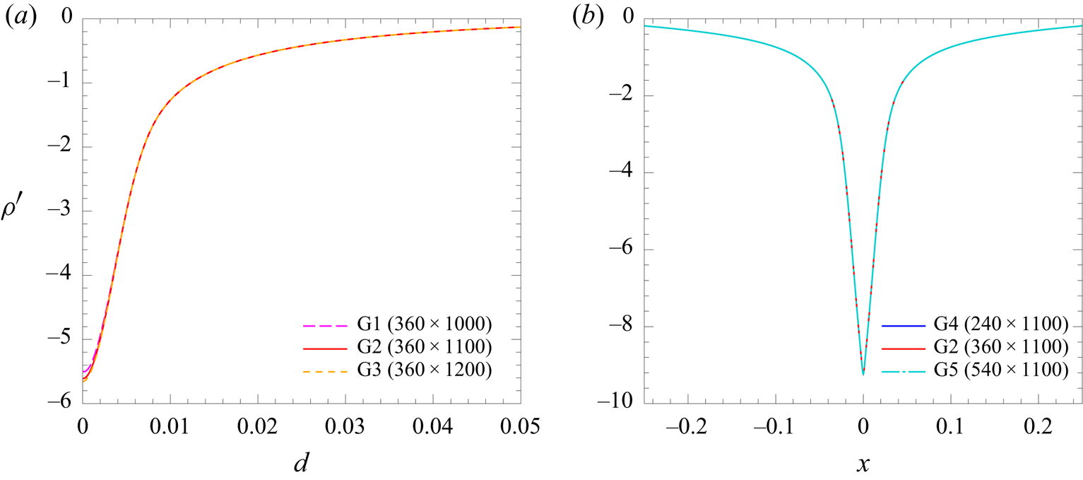
 $1'$ to ensure the accuracy of the numerical simulation more specifically. Five different grids (G1–G5) are tested, and the errors relative to the solution obtained by grid G2 (
 $360 \times 1100$ points), which is actually used in this study, are listed in table 3.
The grid used for the actual computation (grid G2) and the other four grids (G1, G3–G5) with different resolutions. Here,  $\xi _{max}$ and
 $\eta _{max}$ are the number of grid points in the
 $\xi$ and
 $\eta$-directions. The minimum grid spacing in the
 $\xi$-direction appears near the
 $z$-axis, and the minimum grid spacing in the
 $\eta$-direction appears at the sphere surface. The errors relative to the solution obtained by grid G2 (for case C
 $1'$), are listed in the right two columns.

In the top three rows of table 3 (grids G1–G3), the number of grid points in the  $\eta$-direction increases from
 $\eta _{max}=1000$ to
 $1200$, and the minimum grid spacing at the sphere surface decreases from
 $2.81 \times 10^{-4}$ to
 $5.42 \times 10^{-5}$ (less than 1/5 times). Correspondingly, the number of grid points within the scalar boundary layer increases approximately from 5 to 16, while the maximum grid spacing at the outer boundary is unchanged. Figure 11(a) shows the distributions of scalar perturbation on the
 $x$-axis near the equator of the sphere (
 $0.5 \leq x \leq 0.55$ (i.e.
 $0 \leq d \leq 0.05$),
 $y=z=0$), which are obtained by grids G1–G3. The result is almost insensitive to the grid resolution, although the values in the scalar boundary layer (
 $d \lesssim 0.0015$) slightly decrease for finer grids. The difference becomes maximum exactly on the sphere surface (
 $d=0$), but the relative error between the two finer grids G2 and G3 is only 0.83 %, while the minimum grid spacing in grid G3 (
 $5.42\times 10^{-5}$) is less than half of that in grid G2 (
 $1.23\times 10^{-4}$).
Distributions of the scalar perturbation for case C $1'$ obtained by the grids in table 3. (a) Distribution near the equator of the sphere (
 $0.5 \leq x \leq 0.55$ (i.e.
 $0 \le d \le 0.05$) and
 $y=z=0$) obtained by grids G1, G2 and G3. (b) Distribution on the horizontal line across the jet (
 $-0.25 \leq x \leq 0.25$,
 $y=0$ and
 $z=0.8$) obtained by grids G4, G2 and G5.

On the other hand, in grids G4, G2 and G5, the number of grid points in the  $\xi$-direction increases from
 $\xi _{max}=240$ to
 $540$, and the minimum grid spacing near the
 $z$-axis decreases from
 $2.40 \times 10^{-4}$ to
 $1.10 \times 10^{-4}$ (less than 1/2 times). Correspondingly, the number of grid points across the jet, whose radius is estimated by the HWHM of the distribution of
 $\nabla ^{2} \rho ^{\prime }$, increases approximately from 6 to 13. Figure 11(b) shows the scalar distribution across the jet obtained by the grids G4, G2 and G5. The result is insensitive to the grid resolution, with the relative error between gird G2 and G5 being only
 $8.4\times 10^{-4}\%$ (table 3).
Appendix B. The time necessary for the passive-scalar distribution to become steady
The numerical simulation in this study is performed until  $t=10$ for comparison with the experiments. Then, it would be important to note whether the flow has arrived at a steady state or not at
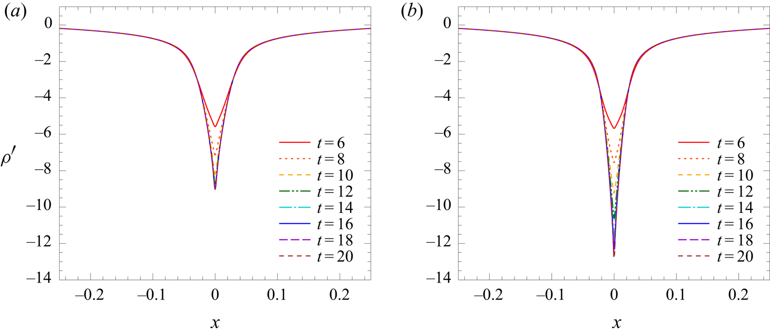
 $t=10$. In general, the velocity distribution becomes steady much earlier than the scalar distribution in the flow for a high Schmidt number, since the diffusion time scale of the scalar is much larger compared with that of velocity, particularly in the scalar boundary layer where the molecular diffusion is significant. Figure 12 shows the time evolution of the passive-scalar distribution on a horizontal line across the jet (
 $y=0,$
 $z=0.8$) for two Schmidt numbers
 $Sc_C=700$ and 2000 (
 $Re=220$,
 $Fr=1$,
 $Sc_S=700$). The time evolution of the passive scalar of
 $Sc_C=700$ (figure 12a) arrives at a steady state at
 $t \sim 10$. This is consistent with the previous numerical study which showed that the density (
 $Sc_S=700$) becomes steady at the upper stagnation point of the sphere at
 $t \sim 10$ (figure 11 of Hanazaki et al. Reference Hanazaki, Nakamura and Yoshikawa2015).
Time evolution of the passive-scalar distribution on a horizontal line across the jet ( $-0.25 \leq x \leq 0.25$,
 $y=0$ and
 $z=0.8$) for different
 $Sc_C$; (a)
 $Sc_C=700$, (b)
 $Sc_C=2000$ (
 $Re=220$,
 $Fr=1$,
 $Sc_S=700$).

On the other hand, for a higher  $Sc_C\, (=2000$, figure 12b), it takes a longer time (
 $t \sim 16$) to reach a steady state, with the generation of a larger peak. Then, the passive-scalar distribution is not yet steady in the jet (
 $z=0.8$) at
 $t=10$. We had better note, however, that the steady state of the scalar in the boundary layer is achieved much earlier at lower heights (e.g. at
 $z=0$) on the sphere surface (cf. figure 13 of Hanazaki et al. Reference Hanazaki, Nakamura and Yoshikawa2015). Then, while figure 5(b), which shows the density across the jet above the sphere (
 $z=0.8$), would show a transient state, figure 4(b), which gives the density near the equator, would show a steady state.
Appendix C. Effects of the thickness and the lateral displacement of the laser light sheet in LIF
We evaluate how the distribution of the fluorescent dye measured by LIF is affected by the non-zero thickness of the laser light sheet and its small lateral displacement from the centre of the jet ( $y=0$), taking case C
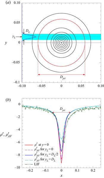
 $1'$ or C1 as an example. Consider a vertical light sheet whose thickness is
 $D_L$, located at
 $y=y_L$ (figure 13a). The intensity of laser light sheet across the sheet is given by
 \begin{equation} I(y)=I_0 \exp \left[{-}2\left(\frac{y-y_L}{D_L/2}\right)^{2} \right] , \end{equation}
when the laser beam has an ordinary Gaussian profile and the peak intensity  $I_0$ is located at
 $y=y_L$. In this study, we actually measured the profile of the laser light sheet in a homogeneous fluid by LIF, and found that
 $D_L^{*} \simeq 0.6$ mm. This means that the non-dimensional thickness is
 $D_L=0.015$ if the sphere diameter is
 $2a^{*}=4$ cm, as in case C
 $1'$.
(a) The distribution of density perturbation  $\rho ^{\prime }$ or
 $C^{\prime }$ on the horizontal plane
 $z=0.8$ for case C
 $1'$. Contours are drawn for
 $\rho ^{\prime }=-1, -2,\ldots , -9$, and the red circle represents the diameter of the jet
 $D_{jet}(=0.12)$. The radius
 $D_{jet}/2(=0.06)$ is determined by the position
 $|x|$ where
 $\rho ^{\prime }$ becomes
 $1/e^{2}$ times its peak value. The blue area shows the laser light sheet with a Gaussian profile (C1) centred at
 $y=y_L$, with thickness
 $D_L$. The non-dimensional value of
 $D_L(=0.015)$ is determined from the direct measurement by LIF. The displacement of the light sheet is tentatively set at
 $y_L=D_L$ for illustration. (b) The distribution of real density perturbation
 $\rho ^{\prime }$ at
 $y=0$ and the three predictions for
 $\rho ^{\prime }_{AV}$ to be observed by a light sheet of non-zero thickness
 $D_L$ located at
 $y_L=0$,
 $D_L/2$ or
 $D_L$. These four distributions are based on the numerical results (case C
 $1'$), and the distribution actually observed by LIF (case C1) is also provided.

The CCD camera observes the fluorescence emitted from the whole width of the light sheet (mostly from  $y_{L}-D_{L}/2 \leq y \leq y_{L}+D_{L}/2$), while we intend to measure the density distribution exactly on the vertical plane
 $y=0$. We then need to estimate the difference between the real fluorescence distribution exactly on
 $y=0$ and that observed by the CCD camera.
For this purpose, we have to consider the combined effect of the axisymmetric distribution of  $\rho ^{\prime }$ (or
 $C^{\prime }$) and the non-uniform intensity of laser light given by (C1). Figure 13(a) shows the axisymmetric distribution of
 $\rho ^{\prime }$ on the horizontal plane of
 $z=0.8$ for case C
 $1'$, i.e. obtained by the numerical simulation. Note that the thickness of the laser light sheet
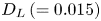 $D_L\,(=0.015)$ is much smaller than the diameter of the jet
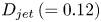 $D_{jet}\,(=0.12)$ indicated by a red circle, suggesting that the effect of non-zero sheet thickness (
 $D_{L} \neq 0$) is small. The effect of
 $y_L\,(\neq 0)$ becomes significant if
 $y_L \gtrsim D_{jet}$, but the value of
 $y_L$ would be usually smaller than
 $D_L$ and thus much smaller than
 $D_{jet}$ (i.e.
 $y_L \lesssim D_L \ll D_{jet}$) in the present LIF. Therefore, the effect of
 $y_L$ would not be significant, as discussed below.
We also note that the effects of  $D_L\neq 0$ and
 $y_L \neq 0$ are negligibly small when we observe the scalar boundary layer on the equator of the sphere as in figure 4, since the diameter of the sphere is equal to 1 and much larger than
 $D_{jet}$, meaning that
 $D_L, y_L\, (\ll D_{jet}) \ll 1$ is well satisfied.
The fluorescence observed by a CCD camera at point  $(x, z)$ can be estimated by
 \begin{align} \rho^{\prime}_{AV}(x, z) &=\left. \int_{-\infty}^{\infty} \rho^{\prime}(x, y, z) I(y) \,{\textrm{d}y} \right/\int_{-\infty}^{\infty} I(y) \,{\textrm{d}y}\nonumber\\ &=\frac{2\sqrt{2}}{\sqrt{\rm \pi}D_L}\int_{-\infty}^{\infty} \rho^{\prime}(x, y, z) \exp \left[{-}2\left(\frac{y-y_L}{D_L/2}\right)^{2} \right] \,{\textrm{d}y}, \end{align}
and the values at the height of  $z=0.8$ for three values of light-sheet displacement
 $y_{L}\,(=0, D_{L}/2 \ \textrm {and} \ D_{L})$ are compared with the real value
 $\rho ^{\prime }\, (x, y=0, z=0.8)$ in figure 13(b).
When  $y_{L}=0$, i.e. when the light sheet passes through the centre of the jet, only
 $D_L\,(\neq 0)$ matters. In this case, distributions of
 $\rho ^{\prime }$ and
 $\rho ^{\prime }_{AV}$ are almost identical except for the very vicinity of
 $x=0$ (i.e.
 $|x| \lesssim D_{L}/2=7.5\times 10^{-3}$) where the peak value of
 $\rho ^{\prime }_{AV}$ is 6.8 % smaller than that of
 $\rho ^{\prime }$. This illustrates that the effect of
 $D_L$ is small if
 $D_L \ll D_{jet}$, as noted above.
When  $y_L=D_L/2=7.5\times 10^{-3}$,
 $\rho ^{\prime }_{AV}$ becomes 12.8 % smaller, in addition to the 6.8 % decrease due to the effect of
 $D_L (\neq 0)$. In this case,
 $\rho ^{\prime }_{AV}$ agrees well with the value actually measured by LIF (case C1) even at its peak (
 $x=0$), suggesting that this
 $y_{L}$
 $(y_{L}^{*}=D_{L}^{*}/2 \simeq 0.3$ mm) is approximately the actual value in the present experiment, although it is difficult to know the exact value of
 $y_L$. We should mention also that the error is smaller for larger
 $|x|$, and the difference between
 $\rho ^{\prime }$ and
 $\rho ^{\prime }_{AV}$ (with
 $y_L=D_L/2$) is less than 10 % for
 $|x|>6.7\times 10^{-3}\,(=0.056D_{jet})$, and less than 5 % for
 $|x|>0.024\,(=0.2D_{jet})$. Therefore, the region with relatively large error is limited to the very central region of the jet.
When  $y_L=D_L$, the observed peak value of
 $\rho ^{\prime }_{AV}$ reduces to approximately 50 % of the peak value of
 $\rho ^{\prime }$, and further increase of
 $y_L\,(>D_L)$ will only lead to more significant reduction. Considering the good agreement for
 $y_L=D_L/2$, it is very unlikely that
 $y_L>D_L$ occurs in the present LIF.
Finally, we should note that the above error estimation assumed the most typical value of 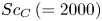 $Sc_C\,(=2000)$. The measurement of the diffusion coefficient is a subtle problem, and the value often varies among the literature in chemistry. In the case of Rhodamine, Troy & Koseff (Reference Troy and Koseff2005) cites
 $Sc_C=600$ as its lowest value. Then if
 $Sc_C=700$ for example, the peak value of
 $|\rho '|$ at
 $x=0$ becomes approximately 10 % lower in the numerical simulation (figure 5), and the maximum error in LIF reduces to approximately 10 %.