



1. Introduction
Supercritical fluids play a significant role in a variety of industrial applications, such as liquid rocket engines (Yang Reference Yang2000; Wang et al. Reference Wang, Wang and Yang2019), regenerative cooling (Xie et al. Reference Xie, Xu, Lei, Li, Li and Sunden2022) and thermal power cycles (White et al. Reference White, Bianchi, Chai, Tassou and Sayma2021; Cao et al. Reference Cao, Xu, He and Jiang2023b
). Fluids at supercritical pressure demonstrate numerous distinctive thermodynamic behaviours, including reduced viscosity, negligible surface tension, enhanced diffusivity and vanishment of the conventional gas–liquid interface (Yang Reference Yang2000; Dahms & Oefelein Reference Dahms and Oefelein2013; Guardone et al. Reference Guardone, Colonna, Pini and Spinelli2024). Additionally, thermodynamic and transport properties exhibit anomalous variations near the critical point and across the pseudo-boiling line (Wan et al. Reference Wan, Wang, Jin and Zhao2025). Figure 1 shows such behaviour using N-dodecane as an example (critical point:1.817 MPa,658.1K). At a pressure close to the critical value of
 $p_r=p_a/p_{cr}=1.01$
, the thermophysical properties of dodecane exhibit pronounced nonlinear variations near the pseudo-boiling point (where the maximum specific heat at constant pressure occurs, approximately at 659K). This behaviour is recognised as the real-fluid effect of supercritical fluids (Zong et al. Reference Zong, Meng, Hsieh and Yang2004; Ding et al. Reference Ding, Li, Wang, Ni and Wang2024a
), which triggers many distinct flow characteristics from the ideal-gas counterpart. Linear stability analysis is a valuable tool to describe the instability evolution and laminar to turbulence transition in fluid flows. However, most existing studies have focused on the stability analysis of ideal gases and have not taken into account real-fluid effects, which are necessary for supercritical flows. To this end, we develop a systematic framework of global linear stability analysis (GLSA) for supercritical fluid flows and further demonstrates its application to a supercritical jet in crossflow (JICF).
Linear stability analysis can be broadly categorised into two types: local linear stability analysis (LLSA) and GLSA (Huerre & Monkewitz Reference Huerre and Monkewitz1990). Local linear stability analysis typically characterises the local impulse response of the system under the parallel-flow assumption at each streamwise location. Several studies (Fu & Yang Reference Fu and Yang2016; Fu et al. Reference Fu, Zhang, Mo and Yang2018; Ren et al. 2018, Reference Ren, Marxen and Pecnik2019; Wang et al. Reference Wang, Liu, Ma and Yang2022) have conducted LLSA on supercritical fluid flows. Ren et al. (Reference Ren, Fu and Pecnik2018) analysed the stability in
 $\mathrm{CO}_{{2}}$
Poiseuille flow at supercritical pressures and identified inflectional profiles in the velocity distribution, attributed to strong property gradients under transcritical conditions. Wang et al. (Reference Wang, Liu, Ma and Yang2022) investigated the stability of a supercritical-pressure nitrogen mixing layer and demonstrated that near the critical point, the maximum spatial growth rate and the most unstable frequency, derived from the real-fluid density profile, are significantly lower than those predicted under the ideal-gas assumption. This discrepancy is explained by the emergence of an inflection point in the density distribution within the mixing layer. Although LLSA has been employed to explore the stability of supercritical fluid flows, the parallel-flow approximation in LLSA is not strictly applicable to flows with distinct three-dimensional characteristics, such as a JICF (or transverse jet), which is frequently employed for fuel injection in advanced propulsion systems.
Property variations of dodecane at different supercritical pressures: (a) density, (b) specific heat capacity at constant pressure, (c) dynamic viscosity, (d) thermal conductivity.

Figure 1. Long description
Four line plots show dodecane properties from 550 to 750 K at reduced pressures pr = 1.01, 1.65 and 3.30. Near-critical pressure produces an abrupt density drop, a sharp heat-capacity peak near 659 K, and steep viscosity and conductivity changes. At pr = 1.65 these transitions broaden and shift to higher temperature; at pr = 3.30 all four properties vary smoothly.
In contrast, GLSA directly deals with the stability characteristics of the entire flow field (Huerre & Monkewitz Reference Huerre and Monkewitz1990; Theofilis Reference Theofilis2011). It was initially introduced in Pierrehumbert & Widnall (Reference Pierrehumbert and Widnall1982) and subsequently found widespread application in the stability analysis of incompressible flows (Obrist & Schmid Reference Obrist and Schmid2003; Barkley Reference Barkley2006; Kervik et al. Reference Kervik, HPffner, Ehrenstein and Henningson2007; Sipp & Lebedev Reference Sipp and Lebedev2007; Bagheri et al. Reference Bagheri, Schlatter, Schmid and Henningson2009; Regan & Mahesh Reference Regan and Mahesh2017; Canton et al. Reference Canton, Auteri and Carini2017). Barkley (Reference Barkley2006) conducted a GLSA of the mean flow arising from laminar vortex shedding behind a circular cylinder across a range of Reynolds numbers (46–180). Results revealed that the eigenfrequency of the mean flow is virtually correlated with the Strouhal number of the vortex shedding. Kervik et al. (Reference Kervik, HPffner, Ehrenstein and Henningson2007) employed a set of two-dimensional global eigenmodes as a projection basis to analyse the flow dynamics and construct a reduced-order model for control applications in a prototype separated boundary-layer flow. An optimal growth analysis demonstrated that a linear combination of these highly non-normal global eigenmodes effectively captures the evolution of localised disturbances. The GLSA of incompressible coaxial jets by Canton et al. (Reference Canton, Auteri and Carini2017) demonstrated that the dominant behaviour of alternating vortex shedding from the duct wall originates from an unstable global mode of the axisymmetric base flow, rather than from the inherent convective nature of jet flow instabilities. As a canonical three-dimensional flow configuration, JICF has also been the subject of GLSA in previous studies.
Jet in crossflow involves a transverse jet injected perpendicularly into a crossflow. This fundamental flow configuration has been extensively investigated over decades, driven by its wide-ranging relevance to propulsion systems in engineering applications (Karagozian Reference Karagozian2010; Mahesh Reference Mahesh2013). Extensive experiments have revealed that the jet’s upstream shear-layer (USL) transitions from convective instability to absolute/global instability as the jet-to-crossflow momentum flux ratio (
 $J$
) gradually decreases (Megerian et al. Reference Megerian, Davitian, De, L. and Karagozian2007; Davitian et al. Reference Davitian, Getsinger, Hendrickson and Karagozian2010; Getsinger et al. Reference Getsinger, Gevorkyan, Smith and Karagozian2014) (with critical
 $J \approx 10$
). Experiments have evidenced that low-amplitude external excitations of JICF with a convectively unstable USL can significantly enhance mixing efficiency (Narayanan et al. Reference Narayanan, Barooah and Cohen2003; Getsinger et al. Reference Getsinger, Hendrickson and Karagozian2012). In the case of global instability, in contrast, high-amplitude excitations prove ineffective in suppressing the dominant instability mode or improving jet penetration and mixing performance (M’Closkey et al. Reference M’Closkey, King, Cortelezzi and Karagozian2002; Shapiro et al. Reference Shapiro, King, M’Closkey and Karagozian2006; Getsinger et al. Reference Getsinger, Hendrickson and Karagozian2012). Linear stability analysis provides further insight into the stability characteristics of JICF. Alves et al. (Reference Alves, Kelly and Karagozian2007, Reference Alves, Kelly and Karagozian2008) and Amini (Reference Amini2018) used LLSA to investigate the shear-layer stability of JICF within the convectively unstable regime and examined the maximum spatial growth rate of disturbances. However, as previously noted, JICF represents a classic three-dimensional flow configuration, rendering the suitability of LLSA to restricted situations. On the other hand, GLSA has shown effectiveness in resolving the intricate USL instabilities of JICF (Bagheri et al. Reference Bagheri, Schlatter, Schmid and Henningson2009; Peplinski et al. Reference Peplinski, Schlatter and Henningson2015; Regan & Mahesh Reference Regan and Mahesh2017). Bagheri et al. (Reference Bagheri, Schlatter, Schmid and Henningson2009) performed a GLSA on a three-dimensional base flow of JICF and revealed the presence of high-frequency unstable global eigenmodes related to shear-layer instabilities on the counter-rotating vortex pair (CVP), as well as low-frequency modes linked to the periodic shedding of vortices in the jet wake. Regan & Mahesh (Reference Regan and Mahesh2017) employed GLSA on JICFs at a jet Reynolds number of
 $\textit{Re}_{\!{j}}=2000$
and captured the transition from global to convective instability in the USL reported by Megerian et al. (Reference Megerian, Davitian, De, L. and Karagozian2007), within the range of velocity ratio (
 $R$
) from 2 to 4. Specifically, the USL instability prevails at
 $R=2$
, while the downstream shear-layer instability becomes predominant at
 $R=4$
. Despite numerous advancements in the literature, the existing GLSA studies on JICF have been mainly conducted at low to moderate pressures with incompressible ideal gas as the working fluid, which cannot be employed to study JICF at supercritical pressures (hereinafter, supercritical JICF) with strong real-fluid effects. Modifications of the base flow and the stability analysis algorithm are necessary to account for real-fluid effects, such as compressibility and abrupt property variations.
Compressibility effects have been considered in numerous studies of the stability analysis of high-speed flows (Schmidt & Rist Reference Schmidt and Rist2011; Kumar et al. Reference Kumar, Bertsch and Girimaji2014; Luo et al. Reference Luo, Li, Ding, Zhai and Si2019; Hao et al. Reference Hao, Cao, Wen and Olivier2021; Cao et al. Reference Cao, Hao, Guo, Wen and Klioutchnikov2023a
; Liu et al. Reference Liu, Chen, Wan, Zhang and Chen2024). Schmidt & Rist (Reference Schmidt and Rist2011) investigated the linear stability of compressible flow within a streamwise corner. They compared base flows at three Mach numbers (
 $Ma$
), corresponding to the incompressible limit, a subsonic regime and a supersonic regime. In the supersonic case, they identified an inviscid corner mode exhibiting odd symmetry. This mode, while absent in the subsonic regime, demonstrated a higher amplification rate than its symmetric counterpart. Through GLSA, Hao et al. (Reference Hao, Cao, Wen and Olivier2021) demonstrated that the shock-induced separated flow in a supersonic flow (Mach 7.7) over a two-dimensional compression corner becomes unstable beyond a specific critical ramp angle. They further reported that while an increase in wall temperature substantially enlarges the separation region, it only leads to a slight increase in the critical angle. These investigations primarily address compressibility effects of ideal gases under high-Mach-number conditions, which, however, differ fundamentally from those considered in the present study, namely, compressibility effects induced by the drastic property variations of real fluids at supercritical pressures, despite low Mach numbers. To the best of the authors’ knowledge, no existing GLSA research has been reported for supercritical fluid flow. Such flow is of great significance in response to the increasing demands for higher thermal efficiency and greater thrust in advanced propulsion systems (Wang et al. Reference Wang, Huo, Unnikrishnan and Yang2018), where the influence of real-fluid effects is critical.
The present study develops a novel GLSA framework for supercritical fluid with detailed treatment of abnormal thermophysical property variations. Real-fluid effects are carefully considered by incorporating a cubic equation of state (EOS) and fundamental thermodynamics and transport theories, which are employed in both the numerical simulation of the base flow and the GLSA governing equations. For demonstration, the framework is implemented to explore the stability characteristics of transverse jets at supercritical pressures.
2. Global linear stability analysis framework for supercritical fluids
Global linear stability analysis investigates the dynamic response of a base flow under external perturbations (Theofilis Reference Theofilis2011). This section first presents the theoretical and numerical formulation for the base flow, then derives the GLSA algorithm for supercritical flows, and concludes with validations of the proposed algorithm.
2.1. Theoretical formulation for base flow
The theoretical framework of the base flow is designed to address supercritical fluid dynamics across a broad spectrum of relevant thermodynamic conditions. In the absence of body forces, the conservation equations of the base flow can be expressed in their primitive form as follows.
Mass:
 \begin{equation} {\frac {{\partial }{\rho }}{{\partial }t}+{\rho }\frac {{\partial }u_{\!j}}{{\partial }x_{\!j}}+u_{\!j}\frac {{\partial }{\rho }}{{\partial }x_{\!j}}=0;} \end{equation}
momentum:
 \begin{equation} {\frac {{\partial }u_i}{{\partial }t}+u_{\!j}\frac {{\partial }u_i}{{\partial }x_{\!j}}+\frac {1}{{\rho }}\frac {{\partial }p}{{\partial }x_i}{-}\frac {1}{{\rho }}\frac {{\partial }{{\tau }_{ij}}}{{\partial }x_{\!j}}=0;} \end{equation}
energy:
 \begin{equation} {{\rho }\frac {{\partial }e}{{\partial }t}+{\rho }u_{\!j}\frac {{\partial }e}{{\partial }x_{\!j}}+p\frac {{\partial }u_{\!j}}{{\partial }x_{\!j}}=\frac {{\partial }q_{\!j}}{{\partial }x_{\!j}}+{\varPhi };} \end{equation}
species:
 \begin{equation} {{\rho }\frac {{\partial }Y_k}{{\partial }t}+{\rho }u_{\!j}\frac {{\partial }Y_k}{{\partial }x_{\!j}}{-}\frac {{\partial }}{{\partial }x_{\!j}}\left ({{\rho }D\frac {{\partial }Y_k}{{\partial }x_{\!j}}}\right )=0.} \end{equation}
Here
 $\rho$
,
 $u$
,
 $p$
and
 $Y_k$
denote density, velocity, pressure and mass fraction of species
 $k$
, respectively. The viscous stress tensor
 $\tau _{ij}$
is defined as
 \begin{equation} { \tau _{ij}=\mu \left (\frac {\partial u_i}{\partial x_{\!j}}+\frac {\partial u_{\!j}}{\partial x_i}-\frac {2}{3}\delta _{ij}\frac {\partial u_l}{\partial x_l}\right )}, \end{equation}
where
 $\mu$
is dynamic viscosity. The bulk viscosity effect is neglected in this study, which is commonly adopted in prior investigations of supercritical fluid flows (Miller et al. Reference Miller, Harstad and Bellan2001; Okong’o & Bellan Reference Okong’o and Bellan2002; Oefelein Reference Oefelein2005; Ren et al. Reference Ren, Fu and Pecnik2018). Here
 $e$
,
 $\varPhi$
,
 $q_{\!j}$
and
 $D$
denote specific internal energy, energy generated by viscous dissipation, heat flux and mass diffusivity, respectively. In this study, only the mass fraction of the jet (
 $Y_1$
) needs to be considered in the governing equations, and the mass fraction of the crossflow (
 $Y_2$
) can be determined as
 \begin{equation} Y_2=1-Y_1. \end{equation}
The internal energy equation given in (2.3) is simplified by neglecting
 $\varPhi$
and reformulated in terms of temperature, i.e.
 \begin{equation} {{\rho }c_v\left ({\frac {{\partial }T}{{\partial }t}+u_{\!j}\frac {{\partial }T}{{\partial }x_{\!j}}}\right )+p\frac {{\partial }u_{\!j}}{{\partial }x_{\!j}}+\frac {{\partial }}{{\partial }x_{\!j}}\left ({{\lambda }\frac {{\partial }T}{{\partial }x_{\!j}}}\right )=0,} \end{equation}
where
 $T$
,
 $c_v$
and
 $\lambda$
denote temperature, specific heat capacity at constant volume and thermal conductivity, respectively.
To close the governing equations above, an EOS is required to describe the thermodynamic relationship between pressure, temperature and volume. This study employs a widely used cubic EOS, i.e. the Peng–Robinson (PR) EOS,
 \begin{equation} p=\frac {R_0T}{V{-}b}{-}\frac {{\alpha }}{V^2+2bV{-}b^2}, \end{equation}
where
 $V$
corresponds to the molar volume and
 $R_0$
signifies the universal gas constant. The parameters
 $\alpha$
and
 $b$
characterise the intermolecular attractive and repulsive forces, respectively. Modelling supercritical fluid flows presents unique challenges due to thermodynamic non-idealities and anomalous transport behaviours. To accurately capture these real-fluid effects, a robust evaluation framework for thermophysical properties is essential. Thermodynamic properties, such as speed of sound and enthalpy, are computed based on fundamental thermodynamic theories coupled with the PR EOS. Here
 $c_v$
is expressed as the sum of an ideal-gas part and a departure function accounting for dense-fluid correction (Meng & Yang Reference Meng and Yang2003):
 \begin{equation} c_v(T, \rho ) = c_{v_0}(T) - \int _{\rho _0}^{\rho } \left [ \frac {T}{\rho ^{2}} \left ( \frac {\partial ^{2} p}{\partial T^{2}} \right )_{\!\rho } \right ]_T d\rho . \end{equation}
The partial derivative
 $ ({{\partial }^{2}}p/{\partial }{T^{2}} )_{\rho }$
in (2.9) is obtained by differentiating the PR EOS, as given in (2.8). Transport properties
 $\lambda$
and
 $\mu$
are calculated as (Yang Reference Yang2000; Huber et al. Reference Huber, Lemmon, Bell and McLinden2022)
 \begin{equation} {{\lambda }(T,{\rho })={{\lambda }_{0}}(T)+{\Delta }{\lambda }(T,{\rho })+{\Delta }{\lambda }_c(T,{\rho }),} \end{equation}
 \begin{equation} {{\mu }\left ({T,{\rho }}\right )={{\mu }_{0}}\left ({T}\right )+{\Delta }{\mu }\left ({T,{\rho }}\right )+{\Delta }{\mu }_c\left ({T,{\rho }}\right )\!.} \end{equation}
In (2.10) and (2.11) the first term corresponds to the contribution in the dilute-gas limit, where only two-body molecular interactions are present and the value can be accurately predicted using kinetic theory. The second term, referred to as the residual contribution, accounts for the effects at elevated densities, including many-body collisions, molecular-velocity correlations and collisional transfer. The third term describes the behaviour in the critical region. Mass diffusivity is evaluated using the Takahashi method, which has been specifically calibrated for high-pressure conditions (Wang & Yang Reference Wang and Yang2017; Wang et al. Reference Wang, Wang and Yang2019). Its formulation can be expressed as
 \begin{equation} (D_{ij} p)^+ = \frac {0.00143 \, T^{1.75}}{M_{ij}^{1/2} \left [ (\varSigma _v)_i^{1/3} + (\varSigma _v)_{\!j}^{1/3} \right ]^2}, \end{equation}
 \begin{equation} {\frac {{D_{ij}}p}{{{\left ({{D_{ij}}p}\right )}^{+}}}=f\left ({T_r,p_r}\right ),} \end{equation}
where
 ${M_{ij}}={{2 ({ ({1/M_i} )+ ({1/M_{\!j}} )} )}^{-1}}$
and
 $(\varSigma _{{v}})_i$
represents the sum of the diffusion volume increments for all constituent elements of component
 $i$
, which can be obtained from reference tables. The dimensionless temperature
 $T_r$
and dimensionless pressure
 $p_r$
are obtained by normalising with respect to their critical values. The function
 $f(T_r,p_r)$
is determined via tabulation based on the graphical data provided in Poling et al. (Reference Poling, Prausnitz and O’Connell2001). Following the described theoretical formulation, these thermodynamic and transport properties are pre-calculated and stored in a table for subsequent high-fidelity simulations to improve computational efficiency.
The theoretical framework aforementioned has been extensively employed in the simulation of supercritical fluid flows (Meng & Yang Reference Meng and Yang2003; Meng et al. Reference Meng, Hsiao, Yang and Shuen2005; Wang et al. Reference Wang, Huo, Unnikrishnan and Yang2018). The numerical solver employs a pressure-based, finite-volume methodology, integrated with the pressure-implicit with splitting of operators algorithm for pressure–velocity coupling. Temporal discretisation is implemented using a bounded second-order implicit scheme, while spatial discretisation is performed with a second-order upwind scheme. The numerical method has been successfully implemented by Ding et al. (Reference Ding, Li, Wang, Ni and Wang2024a , Reference Ding, Li and Wangb ) for JICF at supercritical pressures and the calculated results have been validated against the experimental data reported by Xue et al. (Reference Xue, Gao, Xu, Lin and Sung2011).
2.2. The GLSA algorithm
As previously discussed, the GLSA at supercritical pressures must account for the real-fluid effects induced by abnormal thermophysical variations, whereas the existing GLSA studies are constrained with an ideal-gas assumption in the literature. Consequently, it is essential to develop the governing equations of GLSA suitable for supercritical fluid flows. The derivation process is illustrated in the flowchart presented in figure 2(a). The governing equations are deduced by introducing a small perturbation over the base flow, followed by a linearisation process. Each primitive flow variable
 $q$
is decomposed into two terms: a base state
 $\overline {q}$
and a small perturbation
 $\tilde {q}$
:
 \begin{equation} q=\overline {q}+\tilde {q}. \end{equation}
By substituting (2.14) into (2.1), (2.2), (2.4) and (2.7), and subsequently neglecting higher-order
 $O(\tilde {q}^2)$
terms, the linearised governing equations for the perturbations are obtained as
 \begin{equation} {\frac {{\partial }\tilde {{\rho }}}{{\partial }t}+\tilde {{\rho }}\frac {{\partial }{{\overline {u}}_{\!j}}}{{\partial }x_{\!j}}+\overline {{\rho }}\frac {{\partial }{{\tilde {u}}_{\!j}}}{{\partial }x_{\!j}}+{{\tilde {u}}_{\!j}}\frac {{\partial }\overline {{\rho }}}{{\partial }x_{\!j}}+{{\overline {u}}_{\!j}}\frac {{\partial }\tilde {{\rho }}}{{\partial }x_{\!j}}=0,} \end{equation}
 \begin{equation} \begin{aligned} &\frac {\partial \widetilde {u}_{i}}{\partial t} + \widetilde {u}_{j} \frac {\partial \overline {u}_{i}}{\partial x_{j}} + \overline {u}_{j} \frac {\partial \widetilde {u}_{i}}{\partial x_{j}} - \frac {\widetilde {\rho }}{\overline {\rho }^{2}} \frac {\partial \overline {p}}{\partial x_{i}} + \frac {1}{\overline {\rho }} \frac {\partial \widetilde {p}}{\partial x_{i}} \\ +& \frac {\widetilde {\rho }}{\overline {\rho }^{2}} \left [ \frac {\partial \overline {\mu }}{\partial x_{i}} \left ( \frac {\partial \overline {u}_{i}}{\partial x_{j}} + \frac {\partial \overline {u}_{j}}{\partial x_{i}} - \frac {2}{3} \delta _{ij} \frac {\partial \overline {u}_{i}}{\partial x_{j}} \right ) + \overline {\mu } \left ( \frac {\partial ^{2} \overline {u}_{i}}{\partial x_{j}^{2}} + \frac {\partial ^{2} \overline {u}_{j}}{\partial x_{i} \partial x_{j}} - \frac {2}{3} \frac {\partial ^{2} \overline {u}_{i}}{\partial x_{i}^{2}} \right ) \right ] \\ -& \frac {1}{\rho } \left [ \frac {\partial \overline {\mu }}{\partial x_{j}} \left ( \frac {\partial \widetilde {u}_{i}}{\partial x_{j}} + \frac {\partial \widetilde {u}_{j}}{\partial x_{i}} - \frac {2}{3} \delta _{ij} \frac {\partial \widetilde {u}_{i}}{\partial x_{j}} \right ) + \overline {\mu } \left ( \frac {\partial ^{2} \widetilde {u}_{i}}{\partial x_{j}^{2}} + \frac {\partial ^{2} \widetilde {u}_{j}}{\partial x_{i} \partial x_{j}} - \frac {2}{3} \frac {\partial ^{2} \widetilde {u}_{i}}{\partial x_{i}^{2}} \right ) \right ] = 0, \end{aligned} \end{equation}
 \begin{equation} \begin{aligned} &\frac {{\partial }\tilde {T}}{{\partial }t}+{{\tilde {u}}_{\!j}}\frac {{\partial }\overline {T}}{{\partial }x_{\!j}}+{{\overline {u}}_{\!j}}\frac {{\partial }\tilde {T}}{{\partial }x_{\!j}}+\frac {1}{\overline {{\rho }}\ \overline {c_v}}\left ({\tilde {p}\frac {{\partial }{{\overline {u}}_{\!j}}}{{\partial }x_{\!j}}{-}\frac {\overline {p}\tilde {{\rho }}}{\overline {{\rho }}}\frac {{\partial }{{\overline {u}}_{\!j}}}{{\partial }x_{\!j}}+\overline {p}\frac {{\partial }{{\tilde {u}}_{\!j}}}{{\partial }x_{\!j}}}\right )\\-&\frac {\tilde {{\rho }}}{{{\overline {{\rho }}}^2}\ \overline {c_v}}\left ({\frac {{\partial }\overline {{\lambda }}}{{\partial }x_{\!j}}\frac {{\partial }\overline {T}}{{\partial }x_{\!j}}+\overline {{\lambda }}\frac {{\partial }^2\overline {T}}{{\partial }{x_{\!j}^{2}}}}\right )+\frac {1}{\overline {{\rho }}\ \overline {c_v}}\left ({\frac {{\partial }\overline {{\lambda }}}{{\partial }x_{\!j}}\frac {{\partial }\tilde {T}}{{\partial }x_{\!j}}+\overline {{\lambda }}\frac {{\partial }^2\tilde {T}}{{\partial }{x_{\!j}^{2}}}}\right )=0, \end{aligned} \end{equation}
 \begin{equation} \frac {\partial \widetilde {Y_1}}{\partial t}+\widetilde {u}_{\!j}\frac {\partial \overline {Y_1}}{\partial x_{\!j}}+\overline {u}_{\!j}\frac {\partial \widetilde {Y_1}}{\partial x_{\!j}}+\frac {\tilde {\rho }\overline {D}}{\overline {\rho }^2}\frac {\partial \overline {\rho }}{\partial x_{\!j}}\frac {\partial \overline {Y_1}}{\partial x_{\!j}}-\frac {\overline {D}}{\overline {\rho }}\frac {\partial \tilde {\rho }}{\partial x_{\!j}}\frac {\partial \overline {Y_1}}{\partial x_{\!j}}-\frac {\overline {D}}{\overline {\rho }}\frac {\partial \overline {\rho }}{\partial x_{\!j}}\frac {\partial \widetilde {Y_1}}{\partial x_{\!j}}-\frac {\partial \overline {D}}{\partial x_{\!j}}\frac {\partial \widetilde {Y_1}}{\partial x_{\!j}}-\overline {D}\frac {\partial ^2\widetilde {Y_1}}{\partial x_{\!j}^2}=0. \nonumber\\[3pt] \end{equation}
The vector of perturbed primitive variables can be written as
 $\boldsymbol{\tilde {q}}={ ({\tilde {\rho }\mathrm{,}\tilde {u}\mathrm{,}\tilde {v}\mathrm{,}\tilde {w}\mathrm{,}\tilde {T},\tilde {Y_1}} )}^{\mathrm{T}}$
, according to (2.15)–(2.18). The perturbed pressure
 $\tilde {p}$
is unknown and needs to be solved by perturbing the PR EOS. Before such an operation, the PR EOS is conveniently expressed in terms of the compressibility factor as
 \begin{equation} p=Z\rho RT, \end{equation}
where
 $R$
is the specific gas constant and
 $Z$
represents the compressibility factor. Equation (2.19) is broadly used to represent the concise form of real-fluid EOS, and the substitution of the PR EOS (2.8) leads to a cubic equation of
 $Z$
(Poling et al. Reference Poling, Prausnitz and O’Connell2001; Lopez-Echeverry et al. Reference Lopez-Echeverry, Reif-Acherman and Araujo-Lopez2017). Note that
 $Z$
quantifies the departure from ideal-gas behaviour (
 $Z = 1$
for ideal gases) and exhibits a significant deviation from unity in supercritical fluid flows. Applying perturbations to all thermodynamic variables in (2.19) using (2.14), the perturbed equation after linearisation becomes
 \begin{equation} {\tilde {p}=\overline {Z}\overline {{\rho }}\overline {R}\tilde {T}+\overline {Z}\overline {R}\overline {T}\tilde {{\rho }}+\overline {{\rho }}\overline {R}\overline {T}\tilde {Z}+\overline {Z}\overline {{\rho }}\overline {T}\tilde {R}.} \end{equation}
Here, we neglect the contributions of the last two terms (
 $\tilde {Z}$
and
 $\tilde {R}$
) to the perturbed pressure, because of their relatively small magnitudes compared with perturbed density and temperature. It should be noted that the time-averaged properties
 $\overline {Z}$
and
 $\overline {R}$
are not constant but depend on the local primitive properties. Inserting (2.20) into (2.16) and (2.17) lead to
 \begin{equation} \begin{aligned} &\frac {\partial \widetilde {u}_i}{\partial t} +\widetilde {u}_{\!j} \frac {\partial \overline {u}_i}{\partial x_{\!j}}+\overline {u}_{\!j} \frac {\partial \widetilde {u}_i}{\partial x_{\!j}}-\frac {\tilde {\rho }}{\overline {\rho }^2} \frac {\partial \overline {p}}{\partial x_i}+\overline {Z} \overline {R} \frac {\partial \widetilde {T}}{\partial x_i}+\frac {\overline {Z} \overline {R} \overline {T}}{\overline {\rho }} \frac {\partial \tilde {\rho }}{\partial x_i}\\+&\frac {\tilde {\rho }}{\overline {\rho }^2}\left [\frac {\partial \overline {\mu }}{\partial x_{\!j}}\left (\frac {\partial \overline {u}_i}{\partial x_{\!j}}+\frac {\partial \overline {u}_{\!j}}{\partial x_i}-\frac {2}{3} \delta _{i j} \frac {\partial \overline {u}_i}{\partial x_{\!j}}\right )+\overline {\mu }\left (\frac {\partial ^2 \overline {u}_i}{\partial x_{\!j}^2}+\frac {\partial ^2 \overline {u}_{\!j}}{\partial x_i \partial x_{\!j}}-\right .\right . \left .\left .\frac {2}{3} \frac {\partial ^2 \overline {u}_i}{\partial x_i^2}\right )\right ]\\-& \frac {1}{\overline {\rho }}\left [\frac {\partial \overline {\mu }}{\partial x_{\!j}}\left (\frac {\partial \widetilde {u}_i}{\partial x_{\!j}}+\frac {\partial \widetilde {u}_{\!j}}{\partial x_i}-\frac {2}{3} \delta _{i j} \frac {\partial \widetilde {u}_i}{\partial x_{\!j}}\right )+\overline {\mu }\left (\frac {\partial ^2 \widetilde {u}_i}{\partial x_{\!j}^2}+\frac {\partial ^2 \widetilde {u}_{\!j}}{\partial x_i \partial x_{\!j}}-\frac {2}{3} \frac {\partial ^2 \widetilde {u}_i}{\partial x_i^2}\right )\right ]=0, \end{aligned} \end{equation}
 \begin{equation} \begin{aligned} &\frac {\partial \widetilde {T}}{\partial t} +\widetilde {u}_{\!j} \frac {\partial \overline {T}}{\partial x_{\!j}}+\overline {u}_{\!j} \frac {\partial \widetilde {T}}{\partial x_{\!j}}+\frac {\overline {Z}\ \overline {R} \widetilde {T}}{\overline {c_v}} \frac {\partial \overline {u}_{\!j}}{\partial x_{\!j}}+\frac {\overline {Z} \tilde {\rho } \overline {R}\ \overline {T}}{\overline {\rho }{\overline {c_v}}} \frac {\partial \overline {u}_{\!j}}{\partial x_{\!j}}-\frac {\overline {p} \tilde {\rho }}{\overline {\rho }^2 \overline {c_v}} \frac {\partial \overline {u}_{\!j}}{\partial x_{\!j}}+\frac {\overline {p}}{\overline {\rho }{\overline {c_v}}} \frac {\partial \widetilde {u}_{\!j}}{\partial x_{\!j}}\\-&\frac {\tilde {\rho }}{\overline {\rho }^2 \overline {c_v}}\left (\frac {\partial \overline {\lambda }}{\partial x_{\!j}} \frac {\partial \overline {T}}{\partial x_{\!j}}+\overline {\lambda } \frac {\partial ^2 \overline {T}}{\partial x_{\!j}^2}\right )+\frac {1}{\overline {\rho }{\overline {c_v}}}\left (\frac {\partial \overline {\lambda }}{\partial x_{\!j}} \frac {\partial \widetilde {T}}{\partial x_{\!j}}+ \overline {\lambda } \frac {\partial ^2 \widetilde {T}}{\partial x_{\!j}^2}\right ) =0. \end{aligned} \end{equation}
Equations (2.15), (2.18), (2.21) and (2.22) collectively form a closed system governed by the linearised equations with respect to
 $\boldsymbol{\tilde {q}}={ ({\tilde {{\rho }},\tilde {u},\tilde {{\nu }},\tilde {w},\tilde {T},\tilde {Y_1}} )}^{\mathrm{T}}$
, which takes into account real-fluid effects by involving a real-fluid EOS and a detailed treatment of thermophysical property evaluations. Alternatively, the governing equations can be expressed in a vector form, i.e.
 \begin{equation} \frac {{\partial }\boldsymbol{\tilde {q}}}{{\partial }t}=\boldsymbol{A}\boldsymbol{\tilde {q}}, \end{equation}
where
 $\boldsymbol{A}$
is the linear operator and can be written in the following componentwise form:
 \begin{equation} \boldsymbol{A}={-}\left ({\begin{matrix}{A_{{\rho }{\rho }}}&{A_{{\rho }u}}&{A_{{\rho }v}}&{A_{{\rho }w}}&{A_{{\rho }T}}&{A_{{\rho }Y_1}}\\[3pt] {A_{u{\rho }}}&{A_{uu}}&{A_{uv}}&{A_{uw}}&{A_{uT}}&{A_{uY_1}}\\[3pt] {A_{v{\rho }}}&{A_{vu}}&{A_{vv}}&{A_{vw}}&{A_{vT}}&{A_{vY_1}}\\[3pt] {A_{w{\rho }}}&{A_{wu}}&{A_{wv}}&{A_{ww}}&{A_{wT}}&{A_{wY_1}}\\[3pt] {A_{T{\rho }}}&{A_{Tu}}&{A_{Tv}}&{A_{Tw}}&{A_{TT}}&{A_{TY_1}}\\[3pt] {A_{Y_1{\rho }}}&{A_{Y_1u}}&{A_{Y_1v}}&{A_{Y_1w}}&{A_{Y_1T}}&{A_{Y_1Y_1}}\end{matrix}}\right )\!. \end{equation}
Here
 $A_{ij}$
denotes the coefficient of variable
 $j$
in the governing equation of variable
 $i$
. The complete form, dimensions and discretisation method of
 $\boldsymbol{A}$
are provided in Appendix A. Note that
 $\overline {\mu }$
,
 $\overline {Z}$
,
 $\overline {R}$
,
 $\overline {c_v}$
,
 $\overline {\lambda }$
and
 $\overline {D}$
in these equations represent time-averaged values at each spatial point and depend on the local primitive variables (temperature and density) instead of assigning constant values. They are calculated using the real-fluid property evaluation methods described in § 2.1. The perturbed variables are expressed as the product of
 \begin{equation} \tilde {q}\left ({x,y,z,t}\right )=\hat {q}\left ({x,y,z}\right ){{\rm e}^{{\omega }t}}{,} \end{equation}
where
 $\hat {q}$
and
 $\omega$
are generally complex numbers,
 $\omega =\omega _{{r}}+i\omega _{{i}}$
. The temporal growth rate and the frequency are determined by the real component
 $\omega _{{r}}$
and the imaginary component
 $\omega _{{i}}$
, respectively. Substituting (2.25) into (2.23) results in
 \begin{equation} \omega \boldsymbol{\hat {\boldsymbol{q}}}=\boldsymbol{A}\boldsymbol{\hat {\boldsymbol{q}}}. \end{equation}
Equation (2.26) represents a general formulation of GLSA that is applicable to a wide range of fluid flow problems, where real-fluid effects caused by abnormal property variations are carefully considered. More importantly, it can not only handle supercritical flows with heat transfer and multi-species mixing, but also study compressible and incompressible ideal-gas flows through proper simplifications. For example, the algorithm can be easily degenerated to the physical problems where incompressible fluid is involved. For single-component, isothermal and incompressible flows,
 $\overline {Z}=1$
,
 $\tilde {T}=\tilde {Y_1}=0$
. Equations (2.15) and (2.16) can be simplified as follows:
 \begin{equation} \frac {{\partial }{{\tilde {u}}_{\!j}}}{{\partial }x_{\!j}}=0, \end{equation}
 \begin{equation} \frac {{\partial }{{\tilde {u}}_i}}{{\partial }t}+{{\tilde {u}}_{\!j}}\frac {{\partial }{{\overline {u}}_i}}{{\partial }x_{\!j}}+{{\overline {u}}_{\!j}}\frac {{\partial }{{\tilde {u}}_i}}{{\partial }x_{\!j}}+\frac {1}{{\rho }}\frac {{\partial }\tilde {p}}{{\partial }x_i}{{-}\frac {{\mu }}{{\rho }}\frac {{{\partial }^{2}}{{\tilde {u}}_i}}{{\partial }{x_{\!j}^{2}}}}=0. \end{equation}
As a result, the perturbed vector
 $\tilde {\boldsymbol{q}}$
is simplified as
 ${ ({\tilde {u}\mathrm{,}\tilde {v}\mathrm{,}\tilde {w}\mathrm{,}\tilde {p}} )}^{\mathrm{T}}$
, and the corresponding transformation process is shown in figure 2(b). The linear operator
 $\boldsymbol{A}^*$
takes the following componentwise form:
 \begin{equation} {{{\boldsymbol{A}}^{*}}={-}}\left ({\begin{matrix}{{A_{uu}}}&{{A_{uv}}}&{{A_{uw}}}&{{A_{up}}}\\[3pt] {{A_{vu}}}&{{A_{vv}}}&{{A_{vw}}}&{{A_{vp}}}\\[3pt] {{A_{wu}}}&{{A_{wv}}}&{{A_{ww}}}&{{A}_{wp}}\\[3pt] {{A_{pu}}}&{{A_{pv}}}&{{A_{pw}}}&{{A_{pp}}}\end{matrix}}\right )\!. \end{equation}
The complete form of elemental matrices in (2.29) is provided in Appendix A. For simplicity, the two GLSA algorithms are hereafter referred to as the ‘real-fluid algorithm’ and ‘incompressible-fluid algorithm’, respectively. Figure 3 shows the schematic of complexity comparison between the two algorithms.
Flowchart of GLSA algorithm for (a) real fluids and (b) incompressible fluids.

Figure 2. Long description
Two vertical flowcharts compare GLSA formulations. Panel (a) begins with mass, momentum, energy and species equations, applies variable decomposition and linearization, introduces a real-fluid equation of state and thermophysical derivatives, forms dq’/dt = Aq’, advances with B = exp(Aτ), and applies IRAM. Panel (b) follows the same sequence from incompressible continuity and momentum equations with velocity and pressure perturbations.
Schematic of GLSA classification.

Figure 3. Long description
A three-level schematic classifies global linear stability analysis. Incompressible ideal-gas GLSA is at the top. Adding compressibility effects leads to compressible ideal-gas GLSA in the middle. Adding real-fluid thermophysical properties leads to real-fluid GLSA at the bottom. Downward arrows indicate the progressive increase in physical complexity.
For general three-dimensional flows, the explicit construction of matrix
 $\boldsymbol{A}$
is computationally prohibitive due to its large dimension (
 $O(10^6-10^8)$
). To alleviate the issue, a specialised matrix-free time-stepper method is utilised (Bagheri et al. Reference Bagheri, Schlatter, Schmid and Henningson2009). The time-integration operator
 $\boldsymbol{B}={\rm e}^{\boldsymbol{A}\tau }$
is introduced to serve as a numerical representation for simulating the system of linear equations across a time interval
 $\tau$
. This process converts the most unstable eigenvalues into the most dominant ones, characterised by their maximal magnitude. The eigenvectors of matrices
 $\boldsymbol{A}$
and
 $\boldsymbol{B}$
are identical, whereas the eigenvalues of
 $\boldsymbol{A}(\omega )$
can be derived from the eigenvalues of
 $\boldsymbol{B}$
(denoted as
 $\sigma$
) through the relation
 $\omega =\mathrm{ln}(\sigma )/\tau$
. The computation of the leading (most unstable) eigenvalues and their associated eigenmodes is carried out via the implicitly restarted Arnoldi method (IRAM), utilising the ARPACK software library (Lehoucq et al. Reference Lehoucq, Sorensen and Yang1998). Specifically, the selection of
 $\tau$
involves balancing the time scale dictated by the Nyquist criterion with the need for adequate temporal separation of the Krylov vectors to guarantee convergence in the iterative process (Bagheri et al. Reference Bagheri, Schlatter, Schmid and Henningson2009). Furthermore, determining this time interval necessitates supplementary frequency-domain analysis, such as power spectral density (PSD) analysis and the spectral analysis of proper orthogonal decomposition (POD) modal coefficients. More details about the time-stepper method can be found in Bagheri et al. (Reference Bagheri, Schlatter, Schmid and Henningson2009). The mean flows obtained from the numerical simulations in this study are employed as the base flow for GLSA.
As shown in Appendix A, matrix
 $\boldsymbol{A}$
is of dimension
 $6m\times 6m$
(
 $m$
is the number of sampling grid points), while matrix
 $\boldsymbol{A}^*$
is of dimension
 $4m\times 4m$
. Furthermore, each submatrix block of
 $\boldsymbol{A}$
contains a significantly greater number of components. Thus, the computational cost of the real-fluid algorithm is significantly higher than that of the incompressible-fluid algorithm. Taking the GLSA of a supercritical JICF in this study as an example, using a Dell high-performance workstation (a total of 40 CPUs, each with 2.1 GHz Intel Xeon Gold 5218R), the incompressible-fluid algorithm requires approximately 20 minutes for matrix
 $\boldsymbol{A}$
construction and 4 minutes for eigenvalue decomposition, whereas the real-fluid algorithm takes around 100 minutes and 23 minutes for these operations, respectively.
2.3. Validation
To the authors’ best knowledge, there are no publicly reported GLSA results that account for the real-fluid effects in trans/supercritical fluid flows. Consequently, the reliability of GLSA developed in this study is first validated against the GLSA results for incompressible, equidensity JICF reported by Regan & Mahesh (Reference Regan and Mahesh2017). The jet Reynolds number
 $\textit{Re}_{\!{j}}$
is
 $2000$
(
 $R = 2$
and
 $4$
) with a nozzle exit diameter of 3.81 mm. The nozzle geometry is defined by a fifth-order polynomial. The parameter settings of IRAM are established based on the data provided in the literature. Figure 4(a) first compares the time-averaged transverse velocity profiles at the jet exit (
 $z/d = 0.1$
on the jet-centre plane) obtained from experiment (Megerian et al. Reference Megerian, Davitian, De, L. and Karagozian2007) and present numerical simulation under identical flow conditions (
 $\textit{Re}_{\!{j}} = 2000, R = 2$
). The results demonstrate good agreement, with an average relative deviation of 4.1 %, thereby confirming the reliability of the base flow employed in this study. Figure 4(b) illustrates the eigenvalue spectrum of GLSA, by comparing the results obtained by Regan & Mahesh (Reference Regan and Mahesh2017) with those from the present study. The eigenvalues have been non-dimensionalised, with the growth rate represented as
 ${{\omega }_{{r}}}d/ ({2{\pi }{U_{\text{j,}\textit{max}}}} )$
and the Strouhal number as
 ${{\omega }_{\text{i}}}d/ ({2{\pi }{U_{\text{j,}\textit{max}}}} )$
. Good agreement is achieved at different velocity ratios. For cases with
 $R = 2$
and
 $4$
, the relative deviations in the magnitude of the eigenvalues are 3.8 % and 4.4 %, respectively. These results confirm the validity of the present GLSA algorithm.
(a) Comparison of time-averaged transverse velocity profiles between experiment (Megerian et al. Reference Megerian, Davitian, De, L. and Karagozian2007) and present simulation, measured at
 $z/d = 0.1$
on the jet-centre plane (
 $\textit{Re}_{\!{j}} = 2000, R = 2$
). (b) Eigenvalue spectrum of GLSA for JICF obtained by Regan & Mahesh (Reference Regan and Mahesh2017) and present study.

Figure 4. Long description
Panel (a) plots normalized mean transverse velocity against x/d at z/d = 0.1 for Rej = 2000 and R = 2; the simulation line follows the experimental symbols, with 4.1% average deviation. Panel (b) plots growth rate against Strouhal number for R = 2 and 4. Present eigenvalues closely match Regan and Mahesh, with dominant St near 0.65 and 0.78 and magnitude deviations of 3.8% and 4.4%.
To further validate the reliability of the proposed GLSA algorithm, a comparative analysis is conducted against the GLSA results of a compressible flow reported in the literature (Guiho et al. Reference Guiho, Alizard and Robinet2013). The flow of concern is a separated compressible boundary layer downstream of a bump. The free-stream Mach number is 0.1 and the Reynolds number, based on the inlet boundary layer displacement thickness
 $\delta ^*$
, is 600. The bump height
 $h$
is
 $2\delta ^*$
. The base flow is illustrated in figure 5, with density calculated using the compressible model. The reattachment point is located approximately at
 $x/\delta ^* = 140$
. Figure 6 compares the eigenvalues of the unstable eigenmodes derived from the literature with those computed by the proposed real-fluid GLSA algorithm. The eigenvalues are non-dimensionalised using the displacement thickness and the free-stream velocity. The results show close agreement with those of Guiho et al. (Reference Guiho, Alizard and Robinet2013), with an average relative deviation of 1.2 % in the eigenvalue magnitudes. This consistency further supports the reliability of the proposed algorithm.
Mach number distribution of compressible base flow (
 $Ma = 0.1$
,
 $\textit{Re} = 600$
,
 $h = 2\delta ^*$
).

Figure 5. Long description
A Mach-number contour spans a long x/δ*–y/δ* domain containing a bump of height 2δ* near x/δ* = 25. A low-Mach boundary layer separates over the bump and gradually reattaches near x/δ* = 140, while the outer flow remains close to Ma = 0.1. The contour depicts the compressible base flow used to validate the GLSA formulation.
Eigenvalue spectrum of GLSA for flow behind a 2D bump, obtained by Guiho et al. (Reference Guiho, Alizard and Robinet2013) and present study.

Figure 6. Long description
A scatter plot compares nondimensional eigenvalues for flow behind a two-dimensional bump. Present results and Guiho et al. (2013) follow the same arc across the displayed modes, with frequency approximately 0.06–0.27 and growth rate approximately 0.006–0.020. Present points lie only slightly above the reference points, giving an average eigenvalue-magnitude deviation of 1.2%.
The following section introduces a case study of the supercritical JICF under different conditions to demonstrate the efficacy of the aforementioned GLSA algorithm in analysing the stability of supercritical fluid flows.
3. Case study of supercritical JICF
As mentioned earlier, JICF is a fundamental element for fuel–air mixing and film cooling in advanced propulsion systems. However, a JICF at supercritical pressure complicates the physical processes by introducing strong real-fluid effects. The developed GLSA framework can effectively analyse the stability characteristics of supercritical JICF. To this end, the physical problem under investigation is first delineated and the base-flow solution is briefly presented. Subsequently, the GLSA framework is utilised to systematically investigate the influence of momentum flux ratios and real-fluid effects on the flow stability of supercritical JICF, by deriving the eigenmodes and their corresponding growth rates for small perturbations across various cases. Additionally, as outlined in § 3.3, the aforementioned process further requires the application of techniques such as PSD and POD to determine the time interval
 $\tau$
involved in the time-stepper method.
3.1. Problem description
Figure 7 provides a schematic representation of the computational domain for the base flow, encompassing the regions defined by
 $-8 \leqslant x/d \leqslant 24$
,
 $-8 \leqslant y/d \leqslant 8$
and
 $0 \leqslant z/d \leqslant 24$
in the streamwise, spanwise and transverse directions, respectively. The round jet orifice, with a diameter of
 $d$
= 0.5 mm, is positioned at the origin of the domain. To facilitate the numerical set-up, N-dodecane is chosen as a surrogate of the fuel jet, while oxygen is utilised as the crossflow.
Operating conditions.

Table 1. Long description
The table lists nondimensional operating conditions for cases 1, 2, 3 and A: jet and crossflow temperatures Tj,r and Tc,r, pressure pr, velocity ratio R, density ratio S, momentum-flux ratio J and jet Reynolds number Rej. Cases 1–3 use Tj,r = 0.91 and Tc,r = 1.06; their (pr, R, S, J, Rej) values are (3.30, 0.75, 12.7, 7.1, 2000), (1.65, 0.75, 23.4, 13.2, 2224) and (1.65, 0.55, 23.4, 7.1, 1631). Case A has Tj,r = Tc,r = 2.17, pr = 0.03, R = 2.66, S = 1, J = 7.1 and Rej = 1631.
Schematic of computational domain.

Figure 7. Long description
The three-dimensional domain uses x as streamwise, y as spanwise and z as transverse. A round jet of diameter d = 0.5 mm enters upward through the bottom wall at the origin; crossflow with velocity profile Uc enters from the left. The domain extends 32d downstream, 16d spanwise and 24d vertically, with the jet 8d from the inlet. The bottom is no-slip and the remaining far faces are outlets.
Table 1 summarises the operational parameters, including the jet-to-crossflow velocity ratio (
 $R$
), density ratio (
 $S$
) and momentum flux ratio (
 $J$
) for the selected cases. The jet injection temperature (
 $T_{\!{j}}$
), crossflow temperature (
 $T_{\text{c}}$
) and ambient pressure (
 $p_{\text{a}}$
) are non-dimensionalised with respect to the critical values of the jet:
 \begin{equation} {T_{{j,r}}}=\frac {{T_{{j}}}}{{T_{{cr,j}}}}, \end{equation}
 \begin{equation} {T_{{c,r}}}=\frac {{T_{{c}}}}{{T_{{cr,j}}}}, \end{equation}
 \begin{equation} {p_{{r}}}=\frac {{p_{{a}}}}{{p_{{cr,j}}}}. \end{equation}
The subscript ‘
 $\mathrm{r}$
’ denotes the reduced parameters. In cases 1–3 the jet is at supercritical pressures, whereas the crossflow may not necessarily be, as the ambient pressure in the simulated cases does not always exceed the critical pressure of oxygen. The jet Reynolds numbers (based on jet mean velocity
 $U_{\!{j}}$
and
 $d$
) in each case are set to approximately 2000. A total number of four cases are conducted at various reduced pressures (
 $p_{{r}}$
). Cases 1–3 operate at supercritical pressure (
 $p_{{r}}\gt 1$
), while case A is at atmospheric pressure. Case A is configured with both the jet and crossflow composed of air (
 $J$
= 7.1,
 $\textit{Re}_{\!{j}}$
identical to that of case 3) for comparison. The air density is computed using the compressible ideal-gas law, which will be discussed in detail in § 3.2.
Dynamic mesh adaptation is utilised to facilitate efficient and accurate grid refinement. To resolve the substantial density difference between jet and crossflow, as well as the abrupt density variations caused by temperature gradients within the mixing layer at supercritical pressures, localised mesh refinement is implemented in the vicinity of the jet plume and mixing layer. Additionally, a near-wall grid size of
 $y^+ = 1$
is maintained to ensure the accurate resolution of wall boundary layers. To achieve adequate numerical resolution, the grid system utilised in this study was validated via a grid independence study. Three distinct resolution levels were evaluated, with the grid size at the nozzle exit halved at each successive level. The time-averaged flow profile distributions demonstrated good consistency across all three levels. While the finest resolution level is capable of resolving small-scale eddies, the intermediate level is chosen to balance computational efficiency with numerical accuracy.
Table 2 presents a summary of the axial, radial and azimuthal grid sizes in the intermediate grid system near the nozzle exit, evaluated relative to the Kolmogorov scale, which is computed as
Summary of grid sizes in intermediate grid system near the nozzle exit, normalised by the Kolmogorov scale.

Table 2. Long description
The table gives axial, radial and azimuthal grid-size ranges normalized by the Kolmogorov scale. Case 1: 3.18–6.53, 2.12–6.05 and 5.09–9.85. Case 2: 3.55–7.01, 2.25–6.55 and 5.49–9.41. Case 3: 2.76–5.58, 1.85–5.23 and 4.26–8.33. Case A: 2.94–5.59, 1.75–5.22 and 4.23–8.23. Axial and radial grid sizes remain closest to the Kolmogorov scale in all cases.
 \begin{equation} \eta \approx d\boldsymbol{\cdot }{\textit{Re}_{\!{j}}^{-\frac {3}{4}}}. \end{equation}
Evidently, the grid scales near the jet exit in both axial and radial directions approach the Kolmogorov scale. The final number of grid points after adaptive mesh refinement ranges between 31–38 million across different cases. The governing equations are discretised on a collocated grid. A uniform time step of 0.4
 $\unicode {x03BC}$
s is adopted across all simulations to guarantee the acquisition of temporally precise data. The inlet flow at the jet orifice is characterised by a parabolic velocity profile. The bottom wall is subjected to no-slip and adiabatic boundary conditions. Undesirable wave reflections are minimised by applying non-reflecting boundary conditions at the downstream boundaries, achieved through the extrapolation of primitive variables from the interior domain.
3.2. Base flow
Numerical simulations of the base flows in different cases are performed using the theoretical foundation introduced in § 2.1. Figures 8 and 9 illustrate the instantaneous isosurfaces of Q-criterion at a value of
 $5\times 10^6$
in cases 1–3 from different views, coloured by the jet mass fraction. Distinctive vortical structures are observed. Regions shaded in blue represent oxidiser-enriched mixtures originating from the crossflow, while red regions correspond to fuel-rich mixtures emanating from the jet. Shear-layer vortices, generated by a tangential velocity difference, are prominently observed on the windward side of the jet plume. These are followed by smaller-scale vortices, indicating a transitional or turbulent flow state. Notably, the smaller-scale vortices are more pronounced in case 1 (
 $p_{{r}} = 3.30, J = 7.1$
). With the increase in
 $J$
, the jet penetration depth in case 2 (
 $p_{{r}} = 1.65, J = 13.2$
) is significantly enhanced, which facilitates deeper intrusion of the wake vortices in the transverse direction. Close to the wall, horseshoe vortices and small-scale vortices within the wake zone are observed. The latter are more evident in case 1, indicating a stronger interaction between the jet and the wall. Despite the same
 $J$
as that of case 1, case 3 (
 $p_{{r}} = 1.65, J = 7.1$
) exhibits large vortical structures due to the reduction in
 $\textit{Re}_{\!{j}}$
and the intensified density stratification in the jet’s upstream region at a low supercritical pressure. The shear-layer vortices are diminished, while finger-like, large-scale wake vortices become apparent. These observations indicate that a reduction in ambient pressure induces significant alterations in the flow structures of supercritical JICF.
Instantaneous isosurfaces of
 $Q = 5\times 10^6$
from an isometric view, coloured by the mass fraction of fuel: (a) case 1, (b) case 2, (c) case 3.

Figure 8. Long description
Three oblique Q-criterion isosurfaces compare cases 1–3; color denotes fuel mass fraction from oxidizer-rich blue to fuel-rich red. All show windward shear-layer rolls, a counter-rotating vortex pair, wake vortices and horseshoe vortices. Case 1 contains more small-scale vortices, case 2 penetrates deepest, and case 3 has weaker shear-layer rolls with larger finger-like wake structures.
Instantaneous isosurfaces of
 $Q = 5\times 10^6$
from a top view, coloured by the mass fraction of fuel: (a) case 1, (b) case 2, (c) case 3.

Figure 9. Long description
Top-view Q-criterion isosurfaces compare cases 1–3, colored by fuel mass fraction from blue to red. Case 1 shows a nearly symmetric counter-rotating vortex pair and wake about the jet-center plane, characteristic of global instability. Cases 2 and 3 are visibly asymmetric, consistent with convective instability; case 2 is most elongated, while case 3 contains larger coherent structures.
In the downstream region, a distinct symmetric CVP structure is observed in case 1. As illustrated in the top view of figure 9(a), the transient flow field exhibits near symmetry about the jet-centre plane, which is a characteristic feature of a globally unstable transverse jet (Karagozian Reference Karagozian2014; Gevorkyan et al. Reference Gevorkyan, Shoji, Getsinger, Smith and Karagozian2016). In contrast, as shown in figures 9(b) and 9(c), the transient flow fields in cases 2 and 3 display asymmetry, indicative of convectively unstable transverse jets. This difference seems counter-intuitive since cases 1 and 3 have the same momentum flux ratio. In the following, we explain theoretically the fundamental mechanism underlying the instability characteristics using GLSA.
3.3. Global linear stability analysis – momentum-flux-ratio effects
Prior to examining the global stability of JICF at supercritical pressures, a discussion on the stability of a jet’s USL in air JICF (case A) is first presented as a reference at atmospheric pressure. Power spectral density analysis of the base flow is utilised to identify the dominant frequency of flow-field disturbances, thereby facilitating an informed selection of the time interval
 $\tau$
. Velocity fluctuations are measured at multiple locations within the flow field. Figure 10 presents the PSD of transverse velocity (
 $w$
) fluctuations recorded at various locations along the USL, expressed in terms of normalised coordinates (
 $s/d$
, where
 $s$
represents the distance along the time-averaged jet’s upstream streamline that originates from
 $x/d, z/d = -0.5, 0$
) on the jet-centre plane (
 $y/d = 0$
). Power spectral density is expressed in dB (
 ${S_{{\mathrm{dB}}}}{ ({w} )=10}\log _{10}{ ({{S_{xx}}{ ({w} )}} )}$
, where
 $S_{xx}(w)$
denotes the PSD of
 $w$
). Case A exhibits a dominant common tone instability along the USL, characterised by a Strouhal number (
 $\textit{St}=fd/\overline {U_{\!{j}}}$
) consistently maintained at approximately 0.4, which is indicative of global instability.
The PSD of transverse velocity fluctuations at various locations along the jet’s USL (case A).

Figure 10. Long description
Line spectra show transverse-velocity power spectral density in decibels against Strouhal number at s/d = 0.1–5 along the upstream shear layer in atmospheric case A. Every location has a common dominant peak at St ≈ 0.4 and a weaker harmonic near St ≈ 0.78. The coherent tone persists downstream, indicating global instability of the upstream shear layer.
A global stability analysis is then conducted for case A. It is noteworthy that, as inferred from table 1, the mean jet velocity
 $\overline {U_{\!{j}}}$
is around 47.6 m/s. This results in a variable Mach number up to 0.30 in the flow field, implying that the compressibility effect in the flow is non-negligible and necessitating the use of the compressible ideal-gas law for density calculations. To demonstrate this, the two GLSA algorithms introduced in § 2.2 are carried out. In the real-fluid algorithm, matrix
 $\boldsymbol{A}$
is derived from (2.15), (2.18), (2.21) and (2.22), whereas in the incompressible-fluid algorithm, it is obtained from (2.27) and (2.28). It should be noted that the real-fluid algorithm employed in case A adopts the ideal-gas thermophysical properties to be consistent with the solver for the base flow. This differs slightly from the real-fluid algorithm applied later to JICF at supercritical pressures.
Figure 11 illustrates the most unstable eigenvalues (
 $\textit{St}\approx 0.39$
) derived from real-fluid and incompressible-fluid GLSA algorithms. For the incompressible-fluid algorithm, the instability growth rate is significantly higher, reaching the same order of magnitude as
 $\textit{St}$
. The maximum pressure fluctuation
 ${{({\Delta }p/{p})}}_{\textit{max}}$
and density fluctuation
 ${{(\Delta {\rho }/\rho )}}_{\textit{max}}$
in the flow field are 1.4 % and 1.2 %, respectively, indicating discernible compressible effects. Nonetheless, the incompressible-fluid algorithm leads to a nearly five-fold amplification of the growth rate compared with the real-fluid algorithm. This may seem unexpected, as GLSA applied to a mean flow usually yields eigenvalues characterised by minimal growth rates (Barkley Reference Barkley2006; Turton et al. Reference Turton, Tuckerman and Barkley2015). Wan et al. (Reference Wan, Wang, Jin and Zhao2025) showed that density variations introduce mean density-gradient effects, which tend to weaken the turbulent kinetic energy by damping turbulence production, thereby suppressing the development of flow instabilities. Since the real-fluid algorithm explicitly accounts for the spatial fluctuations of density in the flow field, as illustrated in figure 12, these stabilising effects can be captured in the stability analysis. Consequently, it predicts a low modal growth rate compared with the incompressible-fluid algorithm. The incompressible algorithm fails to incorporate a density fluctuation effect. Furthermore, as illustrated in figure 13(a), the eigenmode of
 $\tilde {w}$
obtained using the real-fluid algorithm exhibits a regular shape, indicative of disturbance propagation along the USL. In comparison, as shown in figure 13(b), the eigenmode from the incompressible-fluid algorithm displays additional small-scale structures, with discontinuous regions of alternating positive and negative values near
 $(x/d, z/d) = (0, 1)$
. This discrepancy likely stems from the intrinsic incompatibility between the base flow
 $(\overline {u},\overline {v},\overline {w},\overline {p})^{\mathrm{T}}$
extracted from the present compressible solver and the incompressible GLSA algorithm.
The GLSA eigenvalue spectrum obtained by real-fluid and incompressible-fluid algorithms for case A.

Figure 11. Long description
The eigenvalue plot shows growth rate against Strouhal number for case A. The real-fluid/compressible formulation and incompressible formulation both identify the most unstable mode at St ≈ 0.39, but the incompressible algorithm predicts a growth rate near 0.28 compared with about 0.06 for the real-fluid algorithm—almost five times larger—demonstrating the error introduced by neglecting density and compressibility effects.
Root mean square (rms) contours of density on the jet-centre plane for case A.

Figure 12. Long description
A jet-center-plane contour maps density RMS over x/d = −2 to 7 and z/d = 0–8. Fluctuations are concentrated in a curved band along the jet’s upstream shear layer, peaking near the nozzle around z/d = 1–2 at up to 0.008 kg/m³, then weakening downstream. The surrounding field remains close to zero, showing that density fluctuations are localized to the mixing layer.
Consequently, when compressible effects become non-negligible, the application of the incompressible-fluid algorithm to compressible base flows could introduce significant errors. Particularly, when the fluid properties of the base flow are evaluated using a real-fluid property framework, the incompressible-fluid algorithm leads to significantly larger errors. This underscores the necessity of utilising the real-fluid algorithm for GLSA implementation for real-fluid base flows, such as JICF at supercritical pressures in this study.
Real part of eigenmodes on the jet-centre plane, obtained by (a) real-fluid and (b) incompressible-fluid algorithms for case A (positive and negative lumps: isocontours of
 $\tilde {w}$
; green lines: isolines of
 $\overline {w}$
= 20 m/s).

Figure 13. Long description
Two jet-center-plane eigenmodes show alternating positive and negative transverse-velocity lobes inside green mean-velocity isolines. Panel (a), from the real-fluid algorithm, forms regular inclined stripes propagating along the upstream shear layer. Panel (b), from the incompressible algorithm, adds discontinuous small-scale lobes near the nozzle, reflecting its incompatibility with the compressible base flow.
The PSD of transverse velocity fluctuations at various locations along the jet’s USL: (a) case 1, (b) case 2.

Figure 14. Long description
Power spectral density is plotted against Strouhal number at s/d = 0.1–6. In case 1, all locations share a strong fundamental peak at St ≈ 0.28 and a harmonic near 0.56, indicating global instability. In case 2, the near-nozzle fundamental is St ≈ 0.37, but downstream spectra shift to a dominant subharmonic at St ≈ 0.19. Case-2 amplitudes are lower, indicating convective instability.
Subsequently, the real-fluid GLSA algorithm is leveraged to conduct a comprehensive stability analysis for cases 1–3. To investigate the impact of the momentum flux ratio on the stability characteristics of JICF at supercritical pressures, a comparative analysis between cases 1 and 2 is carried out. To appropriately determine the time interval
 $\tau$
for GLSA and to clarify the stability of the jet’s USL, figure 14 displays the PSD of transverse velocity fluctuations of the base flow measured at multiple positions along the jet’s USL in cases 1 and 2. A total of 12 500 snapshots were acquired at a time step of 0.4
 $\unicode {x03BC}$
s. Based on the Nyquist–Shannon sampling theorem, this configuration yields a frequency resolution spanning the range of 2–1250 kHz. In case 1 (
 $p_{{r}} = 3.30, J = 7.1$
), a pure tone instability is evident throughout the shear layer, with a dominant Strouhal number consistently around 0.28. This behaviour signifies global instability and closely matches the characteristics observed in case A. In case 2 (
 $p_{{r}} = 1.65$
), as
 $J$
is increased to 13.2, the fundamental mode of JICF demonstrates a shift toward lower frequencies (from
 $\textit{St} = 0.37$
to
 $\textit{St} = 0.19$
). When
 $s/d \gt 3$
, the subharmonic mode becomes dominant, signalling the onset of convective instability. This transition in the dominant instability mode can be attributed to the variation in
 $J$
, which is primarily driven by pressure-induced changes in fluid density. Note that the momentum flux ratios in cases 1 and 2 align with the empirical transition criterion distinguishing global and convective instability, where the critical momentum flux ratio is about 10 (Karagozian Reference Karagozian2014; Getsinger et al. Reference Getsinger, Gevorkyan, Smith and Karagozian2014; Shoji et al. Reference Shoji, Harris, Besnard, Schein and Karagozian2020). Furthermore, the perturbation amplitudes at various locations of the USL in case 1 are larger than those in case 2, indicating a higher degree of flow instability in the former.
Given the identified shift of the dominant frequency in the jet’s USL (case 2), POD is further employed to identify the dominant frequencies of the base flow-field variations across a large spatial domain, which is also useful to ascertain the suitable time interval
 $\tau$
in GLSA. For computational efficiency, the data extracted from the jet-centre plane is utilised, which allows for the effective extraction of flow characteristics associated with shear-layer vortices. The sampling frequency and time interval are maintained consistent with those in the PSD analysis. For a specified flow property, the POD analysis enables the projection of spatiotemporal fluctuations onto an optimal subspace spanning a set of orthogonal spatial functions (POD modes), which minimises the associated L2 error for reconstruction. Additional information on this methodology is available in Berkooz et al. (Reference Berkooz, Holmes and Lumley1993). Figure 15 presents the energy distribution of POD modes for transverse velocity fluctuations in cases 1 and 2, accompanied by the Strouhal numbers of the first two POD modes derived from the frequency spectra of their time-dependent coefficients. In case 1 the dominant POD modes correspond to the fundamental harmonic frequency (
 $\textit{St} = 0.28$
) identified in the PSD analysis, while the dominant POD modes are associated with the subharmonic frequency (
 $\textit{St} = 0.19$
) in case 2.
Energy distribution of POD modes for transverse velocity fluctuations in (a) case 1, (b) case 2.

Figure 15. Long description
Two POD spectra plot modal-energy percentage as red stems and cumulative energy as a black curve against logarithmic mode number. Energy is concentrated in the first paired modes. The leading pair in case 1 corresponds to St = 0.28, while the leading pair in case 2 corresponds to St = 0.19. In both panels, individual modal energy rapidly decays and cumulative energy approaches 100% after several tens of modes.
The GLSA based on the real-fluid algorithm is conducted following the aforementioned analyses. The 30 leading eigenvalues are computed with a maximum residual of
 $1\times 10^{-14}$
. Sixty Arnoldi vectors are generated during each iteration of the IRAM. In case 1, a Strouhal number of 0.28 corresponds to a period of 3.57 non-dimensional time units (normalised by
 $d/{U_{\!{j}}}$
), with the time interval
 $\tau$
set to 1.4 time units, which is less than half of 3.57 time units. In case 2 the period increases to 5.26 time units at
 $\textit{St} = 0.19$
, with
 $\tau$
set to 2.2 time units, which is less than half of 5.26 time units. Notably, the nozzle diameter for fuel injection is typically small (0.5 mm in this study), resulting in a large scaling factor for
 $\tau$
compared with values reported in the literature (Bagheri et al. Reference Bagheri, Schlatter, Schmid and Henningson2009; Regan & Mahesh Reference Regan and Mahesh2017). Nevertheless, the selected time intervals still satisfy the Nyquist criterion.
Figure 16 presents the eigenvalue spectra derived from the GLSA calculations in cases 1 and 2, where the Strouhal numbers of the red dots coincide with the POD modes that exhibit the highest energy contribution. For each case, 100 Arnoldi vectors were solved per iteration within the IRAM. From the final results, a subset of eigenvalues that was selected for presentation exhibit both relatively large magnitudes among the 100 eigenvalues and distinctly different Strouhal numbers. In case 1 the eigenvalue at
 $\textit{St} = 0.28$
dominates and exhibits a significantly higher growth rate than the eigenvalues in case 2, which further corroborates the presence of a higher degree of flow instability in case 1. As shown in figure 16(b), the eigenvalue at
 $\textit{St} = 0.19$
demonstrates a higher growth rate than those associated with the fundamental harmonic frequency (
 $\textit{St} = 0.37$
) in case 2, indicating that the subharmonic mode exerts a more substantial influence on flow-field perturbations. This observation is consistent with the results obtained from the POD analysis.
The GLSA eigenvalue spectrum for (a) case 1, (b) case 2.

Figure 16. Long description
Growth rate–Strouhal spectra compare selected GLSA modes; red circles mark modes matching dominant POD frequencies. Case 1 has a clearly dominant mode at St = 0.28 with growth rate about 0.045. In case 2, the red subharmonic at St = 0.19 grows faster than blue modes near the fundamental St = 0.37, but all case-2 growth rates remain below the dominant case-1 value.
Real part of the eigenmodes on jthe et-centre plane: (a) case 1,
 $\textit{St} = 0.28$
; (b) case 2,
 $\textit{St} = 0.19$
(positive and negative lumps: isocontours of
 $\tilde {w}$
; green lines: isolines of
 $\overline {Y_1}=0.7$
).

Figure 17. Long description
Jet-center-plane eigenmodes appear as alternating positive and negative transverse-velocity lobes within green fuel-mass-fraction isolines. In case 1 at St = 0.28, the lobes originate beside the nozzle and follow the windward shear layer, identifying upstream shear-layer instability. In case 2 at St = 0.19, the localized mode begins farther downstream around z/d = 2–5, identifying downstream shear-layer instability.
Figure 17 illustrates the distribution of the eigenmodes corresponding to the two red dots in figure 16 on the jet-centre plane. The green lines represent the contour of the time-average fuel mass fraction with a value of 0.7. The eigenmode at
 $\textit{St} = 0.28$
in case 1, as depicted in figure 17(a), originates near the jet nozzle exit and represents the upstream shear-layer instability. In contrast, figure 17(b) reveals that the eigenmode at
 $\textit{St} = 0.19$
in case 2 emerges farther downstream, away from the jet nozzle exit, and is associated with the downstream shear-layer instability. These results suggest that the flow-field disturbances of a globally unstable transverse jet (case 1) are primarily driven by the upstream shear-layer instability, whereas for a convectively unstable transverse jet (case 2), the downstream shear-layer instability dominates. This aligns with the findings of Regan & Mahesh (Reference Regan and Mahesh2017).
Interestingly, compared with the eigenmode of the atmospheric-pressure air JICF depicted in figure 13(a), the eigenmodes in figure 17 exhibit two distinct features (as summarised in table 3): (i) the eigenmodes mainly locate on the jet windward side, whereas the eigenmode of the atmospheric-pressure air JICF is intersected by the jet’s potential core region; and (ii) the eigenmodes display localised small-scale structures. These may be due to the intense variations in thermophysical properties within the mixing layer on the jet windward side, which significantly amplify flow disturbances in this region. As documented in the literature (Unnikrishnan et al. Reference Unnikrishnan, Huo, Wang and Yang2021; Ding et al. Reference Ding, Li, Wang, Ni and Wang2024a ), density variations of 1–3 orders of magnitude may occur within a spatial scale of several tens of micrometers in mixing layers involving transcritical or supercritical fluid flows.
Differences in primary stability modes of JICF for incompressible fluids and supercritical real fluids.

Table 3. Long description
The table compares the location and morphology of primary JICF stability modes. For incompressible fluids, the eigenmodes occupy the jet’s potential core and appear as neat parallel stripes. For supercritical real fluids, the modes shift to the jet windward side and form localized small-scale structures, reflecting the influence of strong thermophysical-property gradients in the mixing layer.
The significance of viscosity-related terms for eigenvalues and eigenmodes solved by the GLSA are discussed. For the real-fluid mixing layers of interest in this study, the Reynolds numbers exceed
 $O(10^3)$
. Previous studies (Okongo & Bellan Reference Okongo and Bellan2003; Fedioun & Lardjane Reference Fedioun and Lardjane2005; Wang et al. Reference Wang, Liu, Ma and Yang2022) have suggested that, in linear stability analysis, the influence of viscosity and the associated diffusion terms is negligibly small. To clarify this in the present problem, we also derive a new real-fluid operator neglecting viscous terms, and compare the GLSA results of the two real-fluid operators using the base-flow data from cases 1 and 2. The results indicate that the eigenvalues and their corresponding eigenmodes exhibit only minor variations. Neglecting the diffusion terms leads to a slight increase in the growth rate due to the removal of the viscous dissipation effect. Further details are provided in Appendix B. Additionally, to enable a more detailed quantitative comparison, the time-averaged and fluctuating components of the convection and diffusion terms in the momentum equation are used as examples for comparison. Note that although current GLSA results suggest the influence of viscous and diffusive terms is marginal, this study employs a JICF at a Reynolds number of approximately 2000 solely as a demonstrative case for the proposed GLSA algorithm. When addressing other supercritical fluid flows, particularly those characterised by lower Reynolds numbers and significant viscous effects, omitting viscous and diffusive terms would not be advised.
The subsequent discussion is grounded in vortex dynamics to elucidate the physical mechanisms underlying the GLSA results. The analyses presented in this section demonstrate that, under identical jet-to-crossflow velocity ratios, the stability of the JICF undergoes significant variations due to density changes induced by variations in ambient pressure. At high supercritical pressure (case 1,
 $J = 7.1$
), the flow-field disturbances are governed by the upstream fundamental harmonic instability. In contrast, at low supercritical pressure (case 2,
 $J = 13.2$
), the downstream subharmonic instability becomes the dominant factor influencing the flow-field disturbances. The underlying mechanisms will be further investigated in the subsequent discussion. As illustrated in figure 14(a), the perturbation amplitude in case 1 reaches its maximum near
 $s/d = 3$
, followed by a slight attenuation. This indicates that the perturbation energy is predominantly concentrated in the jet’s upstream region. In the downstream region, higher harmonics emerge due to vortex breakdown, whereas subharmonics are scarcely observed. Therefore, the energy transfer from the fundamental harmonic to subharmonics is suppressed, which aligns with the characteristics of global instability (Strykowski & Niccum Reference Strykowski and Niccum1992). Conversely, in case 2 (figure 14
b), the perturbation amplitude exhibits a gradual amplification along the jet’s upstream streamline, indicating a progressive transfer of energy toward the downstream region. The emergence of subharmonics in the downstream area suggests the occurrence of vortex pairing. This represents energy transfer from smaller to larger scales, which is the characteristic of convective instability (Megerian et al. Reference Megerian, Davitian, De, L. and Karagozian2007; Getsinger et al. Reference Getsinger, Hendrickson and Karagozian2012).
The investigation into the causes of the aforementioned phenomena requires an analysis of the vorticity dynamics in the
 $y$
direction, as shown in figure 18. Due to the high axial velocity of the jet compared with the crossflow, the shear-layer vortices on the jet windward and leeward sides exhibit counterclockwise and clockwise patterns on the jet-centre plane, respectively. These opposing rotational directions are visualised on the contours as distinct blue and red/yellow regions. Along the jet streamline, the shear layer can be categorised into three zones: vortex roll-up, vortex pairing and turbulent breakdown (Chandh et al. Reference Chandh, Emerson and Lieuwen2025). In case 1 (figure 18
a), the vortices maintain relatively high intensity near the jet nozzle exit, and the spacing between adjacent vortex cores downstream is relatively large, which inhibits vortex pairing. However, in case 2 (figure 18
b), the vortex intensity near the nozzle exit is weaker. Clear vortex cores begin to emerge at
 $z/d \approx 2$
, and the close spacing between adjacent vortex cores facilitates vortex pairing. The vortex size exhibits a noticeable increase across the range of
 $2 \lt z/d \lt 4$
. This can be attributed to velocity fluctuations of the vortices, which may cause trailing vortices to catch up with leading vortices (Zong & Yang Reference Zong and Yang2007). As a result, the power spectrum exhibits a distinct subharmonic, accompanied by a shift in dominant frequency, until the vortices eventually break down into a fully turbulent shear layer.
Instantaneous contours of
 $y$
vorticity on the jet-centre plane: (a) case 1, (b) case 2.

Figure 18. Long description
Instantaneous y-vorticity contours compare cases 1 and 2. Case 1 shows strong, repeated windward shear-layer vortices that remain coherent from the nozzle before breaking into turbulence above z/d ≈ 5. Case 2 shows vortex roll-up below z/d ≈ 2, pairing over z/d ≈ 2–4 and turbulent breakdown farther downstream. Opposite-sign vorticity marks the windward and leeward shear layers.
The observed variation in transient vorticity is directly linked to the inherent instabilities within the mixing layer. Given the identical velocity ratio
 $R$
, the propagation velocities of vortices in the jet’s upstream regions in cases 1 and 2 are expected to be comparable. Consequently, the spacing between adjacent vortex cores is influenced by the periodicity of vortex generation. This implies that the vortex generation frequency in the jet’s upstream region of case 2 is higher than that of case 1, which aligns with the data presented in figure 14. Specifically, the Strouhal number of the fundamental harmonic is 0.28 in case 1, whereas it is 0.37 in case 2. Despite the similar shear strengths, which suggest equivalent influences of the Kelvin–Helmholtz instability in these two cases, the observed difference in vortex generation frequencies implies the involvement of additional contributing factors. Notably, as indicated in table 1, the density ratio (
 $S$
) in case 2 is nearly twice that of case 1. This significant disparity raises the necessity of investigating the potential role of Rayleigh–Taylor (R-T) instability in modulating the vortex generation dynamics (Roberts & Jacobs Reference Roberts and Jacobs2015; Li & Soteriou Reference Li and Soteriou2018).
Subsequently, a more quantitative investigation of vortex dynamics is presented, and its connection to GLSA is elucidated. The quantification of vortex dynamics can be effectively accomplished through the application of the transport equation presented as
 \begin{equation} {\frac {D\boldsymbol{{\boldsymbol{\omega }}}}{\textit{Dt}}=(\boldsymbol{{\boldsymbol{\omega }}}\boldsymbol{\cdot }\boldsymbol{\nabla })\boldsymbol{u}{-}(\boldsymbol{\nabla }\boldsymbol{\cdot }\boldsymbol{u})\boldsymbol{{\boldsymbol{\omega }}}{-}\boldsymbol{\nabla }\left ({\frac {1}{{\rho }}}\right )\times \boldsymbol{\nabla }p+\boldsymbol{\nabla }\times \left ({\frac {1}{{\rho }}\boldsymbol{\nabla }\boldsymbol{\cdot }\boldsymbol{{\eta }}}\right )\!,} \end{equation}
where
 $\boldsymbol{\omega }$
denotes the vorticity vector and
 $\boldsymbol{\eta }$
represents the viscous stress tensor. On the right-hand side of the equation, the first term, vortex stretching, and the third term, baroclinic torque, serve as quantitative measures for characterising the magnitudes of the Kelvin–Helmholtz instability and the R–T instability, respectively.
Figure 19 illustrates the spatial distributions of the time-averaged vorticity transport budgets in the
 $y$
direction in case 1 (left) and case 2 (right), normalised by the bulk velocity
 $u_{\!{j}}$
and momentum thickness
 $\theta _0$
at the nozzle exit. The baroclinic torque predominantly exerts its influence within the mixing layer regions. In both cases, given that the jet-to-crossflow density ratio
 $S$
exceeds 10, the baroclinic torque demonstrates significantly greater intensity in the mixing layer regions than vortex stretching. In contrast, vortex stretching prevails in the lower wake region, where intense boundary layer separation and recirculation flow occur. Compared with case 1, the elevated density ratio
 $S$
in case 2 significantly amplifies the dominance of baroclinic torque. This enhancement leads to a significant expansion of its influence regions, both upstream and downstream of the jet. Consequently, the enhanced R-T instability drives an increase in the frequency of the fundamental harmonic. Particularly, under the impact of the R-T instability, a distinct region of alternating positive and negative baroclinic torque is observed in the jet’s downstream mixing layer (
 $3 \lt z/d \lt 6$
) in case 2. This arises due to the formation of multiple CVPs. Furthermore, this region corresponds to the area where the GLSA eigenmode is located, as illustrated in figure 17(b).
Unlike case 1, a subharmonic emerges in the jet’s downstream region in case 2. This phenomenon appears to result from the momentum flux ratio
 $J$
exceeding the critical value of 10. However, the present GLSA results reveal that the underlying cause of this transition is attributed to the decrease in ambient pressure, which enlarges the density ratio
 $S$
. The analyses of vortex dynamics further corroborate that this change amplifies the R-T instability, leading to the formation of a subharmonic in the jet downstream region. This mechanism distinctly differs from that reported in the literature, where subharmonics are induced by enhancing the K-H instability through an increase in the velocity ratio
 $R$
(Megerian et al. Reference Megerian, Davitian, De, L. and Karagozian2007; Iyer & Mahesh Reference Iyer and Mahesh2016).
Spatial distributions of time-averaged vortex transport budgets in the
 $y$
direction of case 1 (left) and case 2 (right), normalised by bulk velocity and momentum thickness at the nozzle exit
 ${{({\overline {{u_{j}}}/{\theta }_0})}^2}$
: (a) baroclinic torque, (b) vortex stretching.

Figure 19. Long description
Four contours compare case 1 on the left and case 2 on the right. Row (a) shows baroclinic torque concentrated in the jet mixing layers; case 2 has stronger, broader alternating signs along the downstream layer from z/d ≈ 3–6. Row (b) shows vortex stretching, strongest near the lower wake and nozzle and weaker aloft. Baroclinic torque dominates the shear layers, especially at the higher density ratio of case 2.
3.4. Global linear stability analysis – real-fluid effects
As discussed in § 3.2, the intensified real-fluid effects at a low supercritical pressure (
 $p_{{r}} = 1.65$
), which results from pronounced density stratification, exerts a significant influence on the dynamics of supercritical JICF. To further explore the stability characteristics at low supercritical pressure, case 3 is established by reducing
 $J$
from 13.2 to 7.1 (according to case 1).
As discussed in the previous section, the time interval
 $\tau$
in case 3 for GLSA is first determined. Figure 20(a) illustrates that in case 3, the characteristic frequency of the perturbations along the jet’s upstream streamline undergoes a noticeable shift, mimicking the characteristics of a convective instability. The Strouhal number of the fundamental harmonic is 0.25, which is consistent with the first two POD modes in figure 20(b). At
 $s/d = 4$
, the flow is in a transitional state, while at
 $s/d = 5$
and
 $6$
, the dominant frequency shifts to higher harmonics. Compared with case 1 in figure 14(a), the perturbation amplitudes in figure 20(a) are reduced. Additionally, the perturbation amplitude generally amplifies along the jet’s upstream streamline, although a slight decrease is observed during frequency shifting. This suggests that energy is gradually transferred downstream. However, unlike the convectively unstable JICF observed in case 2 and at subcritical pressures (Megerian et al. Reference Megerian, Davitian, De, L. and Karagozian2007; Getsinger et al. Reference Getsinger, Gevorkyan, Smith and Karagozian2014), no subharmonic emerges downstream. Instead, the dominant frequency progressively shifts to higher harmonics that are generated due to vortex breakdown downstream, implying that energy is transferred to smaller scales. This phenomenon can be attributed to the reduced velocity difference in the shear layer due to the decreased jet velocity in comparison to case 2, which results in a lower vortex generation frequency and an extended spacing between adjacent vortex cores. Additionally, the pronounced density stratification also suppresses vortex pairing (Zong et al. Reference Zong, Meng, Hsieh and Yang2004), making the formation of subharmonics more unlikely.
Stability analysis of case 3: (a) PSD of transverse velocity fluctuations at various locations along the jet’s USL, (b) energy distribution of POD modes for transverse velocity fluctuations.

Figure 20. Long description
Panel (a) plots power spectral density against Strouhal number along the upstream shear layer: the fundamental is St ≈ 0.25 near the nozzle, while downstream locations shift toward a harmonic near St ≈ 0.50 rather than a subharmonic. Panel (b) shows POD energy concentrated in the first paired modes at St = 0.25, with cumulative energy approaching 100%. Perturbation amplitudes are lower than in case 1.
The GLSA eigenvalue spectrum for cases 1 (hollow symbols) and 3 (solid symbols).

Figure 21. Long description
The eigenvalue spectrum plots growth rate against Strouhal number. Case 1 uses hollow symbols and has a dominant red mode near St = 0.28 with growth rate about 0.045. Case 3 uses solid symbols: its fundamental at St = 0.25 grows at about 0.036, and its harmonic at St = 0.50 grows at about 0.025. The reduced case-3 growth rates indicate stabilization by stronger real-fluid effects and density stratification.
The GLSA eigenvalue spectrum for case 3 is presented in figure 21. In case 3,
 $\textit{St} = 0.25$
corresponds to a period of 4, with
 $\tau$
set to 1.7 time units. Compared with the GLSA eigenvalues observed in case 1 (figure 16
a), those in case 3 manifest diminished growth rates, which provide quantitative evidence that the enhanced real-fluid effects induced by pronounced density stratification stabilise the USL of the transverse jet at decreased supercritical pressure. This stabilisation may lead to an anomalous transition in the stability. Figure 22 depicts the spatial distribution of the eigenmodes in case 3 on the jet-centre plane. The eigenmode corresponding to
 $\textit{St} = 0.25$
originates in close proximity to the nozzle exit, characterising the upstream shear-layer instability. Meanwhile, the eigenmode associated with
 $\textit{St} = 0.50$
emerges further downstream with a shorter wavelength and represents a downstream shear-layer instability.
The results of GLSA are further elucidated through vortex dynamics. Figure 23 presents the instantaneous contour of
 $y$
vorticity on the jet-centre plane in case 3. Compared with cases 1 and 2 (figure 18), the weak vortex intensity in the flow field necessitates a narrow colourbar range to clearly visualise the vorticity. As indicated by the red circle, vortex breakdown occurs at
 $z/d \approx 4$
, leading to a frequency shift shown in figure 20(a). Its location coincides with the eigenmode identified in figure 22(b). In comparison to case 1, while the momentum flux ratio
 $J$
remains identical, the density ratio
 $S$
in case 3 increases, resulting in an enhanced R-T instability. However, the reduced velocity difference weakens the K-H instability within the shear layer. Consequently, under the coupled influence of these two factors, the Strouhal numbers of the fundamental harmonic in both cases are similar, with
 $\textit{St} = 0.28$
in case 1 and
 $\textit{St} = 0.25$
in case 3.
Real part of the eigenmodes on the jet-centre plane for case 3: (a)
 $\textit{St} = 0.25$
, (b)
 $\textit{St} = 0.50$
(positive and negative lumps: isocontours of
 $\tilde {w}$
; green lines: isolines of
 $\tilde {Y_1}=0.7$
).

Figure 22. Long description
Two case-3 jet-center-plane eigenmodes appear as alternating positive and negative transverse-velocity lobes within green fuel-mass-fraction isolines. At St = 0.25, panel (a), the long-wave mode begins at the nozzle and follows the upstream shear layer to z/d ≈ 3. At St = 0.50, panel (b), a shorter-wave localized mode begins farther downstream around z/d = 2–4.5, marking downstream shear-layer instability.
Instantaneous contours of the
 $y$
vorticity on the jet-centre plane for case 3.

Figure 23. Long description
An instantaneous y-vorticity contour shows weak alternating-sign shear-layer vortices rising along the windward jet boundary. A red circle marks vortex breakdown near x/d ≈ 0.7 and z/d ≈ 4; above this point, elongated small-scale structures spread downstream. Vorticity is weaker than in cases 1 and 2, with a range of −1.5 to 1.5 × 10^4 s⁻¹, consistent with reduced jet velocity and strong density stratification.
4. Conclusion
The GLSA framework capable of incorporating real-fluid effects in supercritical fluid flows is proposed for the first time. It accounts for real-fluid effects via a cubic EOS and the detailed treatment of real-fluid thermodynamic and transport properties. Furthermore, it incorporates the energy and species transport equations within a unified set of linearised governing equations. As a representative example, the GLSA framework is employed to systematically investigate the stability characteristics of jets in crossflow at supercritical pressures. The base flows in GLSA are obtained through a unified numerical framework for real-fluid flow dynamics. By integrating the implicitly restarted Arnoldi iteration method with a time-stepper approach, this study elucidates the instability dynamics at jet Reynolds numbers of around 2000, with comparative insights drawn from an atmospheric-pressure air JICF case.
The results highlight that adopting an incompressible-fluid algorithm for compressible base flows yields anomalously increased growth rates, particularly when real-fluid effects are consequential. The GLSA framework successfully resolves the complex USL instabilities, with Strouhal numbers aligning closely with PSD analyses and POD results. It permits a more quantitative stability assessment and allows for the intuitive visualisation of eigenmodes. With a same jet-to-crossflow velocity ratio of 0.75, a decrease in ambient pressure can induce the transition of the eigenmode from originating near the nozzle exit to emerging farther downstream, while exhibiting a substantial decrease in growth rate magnitude. This corresponds to a shift of the USL from global to convective instability. The vorticity transport budget analysis demonstrates that this pressure reduction also amplifies R-T instabilities in the mixing layer. This mechanism facilitates downstream vortex pairing, promoting subharmonic formation. These observations underscore the significance of reduced pressure (
 $p_{{r}}$
) as an additional governing parameter at supercritical pressures, except for the jet-to-crossflow momentum flux ratio (
 $J$
), as it arises from the intensified real-fluid effects driven by pronounced density stratification near the critical pressure. Moreover, in this case (
 $J = 7.1,p_{{r}}= 1.65$
), subharmonics are not observed in the jet’s downstream region, which could be due to the reduced velocity difference in the shear layer, along with the significant density stratification that inhibits vortex pairing.
The novel real-fluid GLSA framework is extendable to stability analyses of various supercritical fluid flows. Given the continuous progression toward elevated operational pressures in propulsion and power-generation systems, this research offers a solid theoretical and technical foundation for advanced combustor design.
Acknowledgements
The authors thank Dr Dongjun Ma and Dr Chuhan Wang for their advice on linear stability analysis.
Funding
This work was sponsored by the National Natural Science Foundation of China (52276123).
Declaration of interests
The authors report no conflict of interest.
Appendix A. Linear operator
 $ \boldsymbol{A}$

As mentioned in § 2.2, for the real-fluid algorithm,
 $\boldsymbol{\tilde {q}}={{ ({\tilde {{\rho }},\tilde {u},\tilde {{\nu }},\tilde {w},\tilde {T},\tilde {Y_1}} )}^{\mathrm{T}}}$
. Transforming equations (2.15), (2.18), (2.21, and (2.22) into the form of (2.23) yields the complete expression for
 $\boldsymbol{A}$
, which is a matrix of size
 $6m\times 6m$
, where
 $m$
denotes the number of sampling grid points. The columns of the matrix are structured as follows (for simplicity, the overbar symbols of
 $\overline {\mu }$
,
 $\overline {Z}$
,
 $\overline {R}$
,
 $\overline {c_v}$
,
 $\overline {\lambda }$
and
 $\overline {D}$
have been omitted):
 \begin{equation} {\tiny \left (\!\! \begin{array}{c} A_{\rho \rho } \\[7pt] A_{u \rho } \\[7pt] A_{v \rho } \\[7pt] A_{w \rho } \\[7pt] A_{T \rho } \\[7pt] A_{Y_1 \rho } \end{array} \!\! \right )=\left (\!\!\!\! \begin{array}{c} \dfrac {\partial \overline {u}}{\partial x}+\dfrac {\partial \overline {v}}{\partial y}+\dfrac {\partial \overline {w}}{\partial z}+\overline {u} \dfrac {\partial }{\partial x}+\overline {v} \dfrac {\partial }{\partial y}+\overline {w} \dfrac {\partial }{\partial z} \\[11pt] -\dfrac {1}{\overline {\rho }^2} \dfrac {\partial \overline {p}}{\partial x}+\dfrac {Z R \overline {T}}{\overline {\rho }} \dfrac {\partial }{\partial x} +\dfrac {1}{\overline {\rho }^2} \left ( \dfrac {4}{3} \dfrac {\partial \mu }{\partial x} \dfrac {\partial \overline {u}}{\partial x} + \dfrac {\partial \mu }{\partial y} \dfrac {\partial \overline {u}}{\partial y} + \dfrac {\partial \mu }{\partial y} \dfrac {\partial \overline {v}}{\partial x} + \dfrac {\partial \mu }{\partial z} \dfrac {\partial \overline {u}}{\partial z} + \dfrac {\partial \mu }{\partial z} \dfrac {\partial \overline {w}}{\partial x} \right ) +\dfrac {\mu }{\overline {\rho }^2} \left ( \dfrac {4}{3} \dfrac {\partial ^2 \overline {u}}{\partial x^2} + \dfrac {\partial ^2 \overline {u}}{\partial y^2} + \dfrac {\partial ^2 \overline {v}}{\partial x \partial y} + \dfrac {\partial ^2 \overline {u}}{\partial z^2} + \dfrac {\partial ^2 \overline {w}}{\partial x \partial z} \right ) \\[11pt] -\dfrac {1}{\overline {\rho }^2} \dfrac {\partial \overline {p}}{\partial y}+\dfrac {Z R \overline {T}}{\overline {\rho }} \dfrac {\partial }{\partial y} +\dfrac {1}{\overline {\rho }^2} \left ( \dfrac {\partial \mu }{\partial x} \dfrac {\partial \overline {v}}{\partial x} + \dfrac {\partial \mu }{\partial x} \dfrac {\partial \overline {u}}{\partial y} + \dfrac {4}{3} \dfrac {\partial \mu }{\partial y} \dfrac {\partial \overline {v}}{\partial y} + \dfrac {\partial \mu }{\partial z} \dfrac {\partial \overline {v}}{\partial z} + \dfrac {\partial \mu }{\partial z} \dfrac {\partial \overline {w}}{\partial y} \right ) +\dfrac {\mu }{\overline {\rho }^2} \left ( \dfrac {\partial ^2 \overline {v}}{\partial x^2} + \dfrac {\partial ^2 \overline {u}}{\partial y \partial x} + \dfrac {4}{3} \dfrac {\partial ^2 \overline {v}}{\partial y^2} + \dfrac {\partial ^2 \overline {v}}{\partial z^2} + \dfrac {\partial ^2 \overline {w}}{\partial y \partial z} \right ) \\[11pt] -\dfrac {1}{\overline {\rho }^2} \dfrac {\partial \overline {p}}{\partial z}+\dfrac {Z R \overline {T}}{\overline {\rho }} \dfrac {\partial }{\partial z} +\dfrac {1}{\overline {\rho }^2} \left ( \dfrac {\partial \mu }{\partial x} \dfrac {\partial \overline {w}}{\partial x} + \dfrac {\partial \mu }{\partial x} \dfrac {\partial \overline {u}}{\partial z} + \dfrac {\partial \mu }{\partial y} \dfrac {\partial \overline {w}}{\partial y} + \dfrac {\partial \mu }{\partial y} \dfrac {\partial \overline {v}}{\partial z} + \dfrac {4}{3} \dfrac {\partial \mu }{\partial z} \dfrac {\partial \overline {w}}{\partial z} \right ) +\dfrac {\mu }{\overline {\rho }^2} \left ( \dfrac {\partial ^2 \overline {w}}{\partial x^2} + \dfrac {\partial ^2 \overline {u}}{\partial z \partial x} + \dfrac {\partial ^2 \overline {w}}{\partial y^2} + \dfrac {\partial ^2 \overline {v}}{\partial z \partial y} + \dfrac {4}{3} \dfrac {\partial ^2 \overline {w}}{\partial z^2} \right ) \\[11pt] \left (\dfrac {Z R \overline {T}}{\overline {\rho } c_v}-\dfrac {\overline {p}}{\overline {\rho }^2 c_v}\right )\left (\dfrac {\partial \overline {u}}{\partial x}+\dfrac {\partial \overline {v}}{\partial y}+\dfrac {\partial \overline {w}}{\partial z}\right )-\dfrac {\lambda }{\overline {\rho }^2 c_v}\left (\dfrac {\partial ^2 \overline {T}}{\partial x^2}+\dfrac {\partial ^2 \overline {T}}{\partial y^2}+\dfrac {\partial ^2 \overline {T}}{\partial z^2}\right )-\dfrac {1}{\overline {\rho }^2 c_v}\left (\dfrac {\partial \lambda }{\partial x} \dfrac {\partial \overline {T}}{\partial x}+\dfrac {\partial \lambda }{\partial y} \dfrac {\partial \overline {T}}{\partial y}+\dfrac {\partial \lambda }{\partial z} \dfrac {\partial \overline {T}}{\partial z}\right ) \\[11pt] \dfrac {D}{\overline {\rho }^2}\left (\dfrac {\partial \overline {\rho }}{\partial x} \dfrac {\partial \overline {Y_1}}{\partial x}+\dfrac {\partial \overline {\rho }}{\partial y} \dfrac {\partial \overline {Y_1}}{\partial y}+\dfrac {\partial \overline {\rho }}{\partial z} \dfrac {\partial \overline {Y}_1}{\partial z}\right )-\dfrac {D}{\overline {\rho }}\left (\dfrac {\partial }{\partial x} \dfrac {\partial \overline {Y_1}}{\partial x}+\dfrac {\partial }{\partial y} \dfrac {\partial \overline {Y_1}}{\partial y}+\dfrac {\partial }{\partial z} \dfrac {\partial \overline {Y_1}}{\partial z}\right ) \end{array} \!\!\!\!\right ),} \end{equation}
 \begin{equation} \left (\begin{array}{c} A_{\rho u} \\[7pt] A_{u u} \\[7pt] A_{v u} \\[7pt] A_{w u} \\[7pt] A_{T u} \\[7pt] A_{Y_1 u} \end{array}\right )=\left (\begin{array}{c} \overline {\rho } \dfrac {\partial }{\partial x}+\dfrac {\partial \overline {\rho }}{\partial x} \\[11pt] \dfrac {\partial \overline {u}}{\partial x}+\overline {u} \dfrac {\partial }{\partial x}+\overline {v} \dfrac {\partial }{\partial y}+\overline {w} \dfrac {\partial }{\partial z}-\dfrac {\mu }{\overline {\rho }}\left (\dfrac {4}{3} \dfrac {\partial ^2}{\partial x^2}+\dfrac {\partial ^2}{\partial y^2}+\dfrac {\partial ^2}{\partial z^2}\right )-\dfrac {4}{3 \overline {\rho }} \dfrac {\partial \mu }{\partial x} \dfrac {\partial }{\partial x}-\dfrac {1}{\overline {\rho }} \dfrac {\partial \mu }{\partial y} \dfrac {\partial }{\partial y}-\dfrac {1}{\overline {\rho }} \dfrac {\partial \mu }{\partial z} \dfrac {\partial }{\partial z} \\[11pt] \dfrac {\partial \overline {v}}{\partial x}-\dfrac {\mu }{\overline {\rho }} \dfrac {\partial ^2}{\partial y \partial x}-\dfrac {1}{\overline {\rho }} \dfrac {\partial \mu }{\partial x} \dfrac {\partial }{\partial y} \\[11pt] \dfrac {\partial \overline {w}}{\partial x}-\dfrac {\mu }{\overline {\rho }} \dfrac {\partial ^2}{\partial z \partial x}-\dfrac {1}{\overline {\rho }} \dfrac {\partial \mu }{\partial x} \dfrac {\partial }{\partial z} \\[11pt] \dfrac {\partial \overline {T}}{\partial x}+\dfrac {\overline {p}}{\overline {\rho } c_v} \dfrac {\partial }{\partial x} \\[11pt] \dfrac {\partial \overline {Y_1}}{\partial x} \end{array}\right ), \end{equation}
 \begin{equation} \left (\begin{array}{c} A_{\rho v} \\[7pt] A_{u v} \\[7pt] A_{v v} \\[7pt] A_{w v} \\[7pt] A_{T v} \\[7pt] A_{Y_1 v} \end{array}\right )=\left (\begin{array}{c} \overline {\rho } \dfrac {\partial }{\partial y}+\dfrac {\partial \overline {\rho }}{\partial y} \\[11pt] \dfrac {\partial \overline {u}}{\partial y}-\dfrac {\mu }{\overline {\rho }} \dfrac {\partial ^2}{\partial x \partial y}-\dfrac {1}{\overline {\rho }} \dfrac {\partial \mu }{\partial y} \dfrac {\partial }{\partial x} \\[11pt] \dfrac {\partial \overline {v}}{\partial y}+\overline {u} \dfrac {\partial }{\partial x}+\overline {v} \dfrac {\partial }{\partial y}+\overline {w} \dfrac {\partial }{\partial z}-\dfrac {\mu }{\overline {\rho }}\left (\dfrac {\partial ^2}{\partial x^2}+\dfrac {4}{3} \dfrac {\partial ^2}{\partial y^2}+\dfrac {\partial ^2}{\partial z^2}\right )-\dfrac {1}{\overline {\rho }} \dfrac {\partial \mu }{\partial x} \dfrac {\partial }{\partial x}-\dfrac {4}{3 \overline {\rho }} \dfrac {\partial \mu }{\partial y} \dfrac {\partial }{\partial y}-\dfrac {1}{\overline {\rho }} \dfrac {\partial \mu }{\partial z} \dfrac {\partial }{\partial z} \\[11pt] \dfrac {\partial \overline {w}}{\partial y}-\dfrac {\mu }{\overline {\rho }} \dfrac {\partial ^2}{\partial z \partial y}-\dfrac {1}{\overline {\rho }} \dfrac {\partial \mu }{\partial y} \dfrac {\partial }{\partial z} \\[11pt] \dfrac {\partial \overline {T}}{\partial y}+\dfrac {\overline {p}}{\overline {\rho } c_v} \dfrac {\partial }{\partial y} \\[11pt] \dfrac {\partial \overline {Y_1}}{\partial y} \end{array}\right ), \end{equation}
 \begin{equation} \left (\begin{array}{c} A_{\rho w} \\[7pt] A_{u w} \\[7pt] A_{v w} \\[7pt] A_{w w} \\[7pt] A_{T w} \\[7pt] A_{Y_1 w} \end{array}\right )=\left (\begin{array}{c} \overline {\rho } \dfrac {\partial }{\partial z}+\dfrac {\partial \overline {\rho }}{\partial z} \\[11pt] \dfrac {\partial \overline {u}}{\partial z}-\dfrac {\mu }{\overline {\rho }} \dfrac {\partial ^2}{\partial x \partial z}-\dfrac {1}{\overline {\rho }} \dfrac {\partial \mu }{\partial z} \dfrac {\partial }{\partial x} \\[11pt] \dfrac {\partial \overline {v}}{\partial z}-\dfrac {\mu }{\overline {\rho }} \dfrac {\partial ^2}{\partial y \partial z}-\dfrac {1}{\overline {\rho }} \dfrac {\partial \mu }{\partial z} \dfrac {\partial }{\partial y} \\[11pt] \dfrac {\partial \overline {w}}{\partial z}+\overline {u} \dfrac {\partial }{\partial x}+\overline {v} \dfrac {\partial }{\partial y}+\overline {w} \dfrac {\partial }{\partial z}-\dfrac {\mu }{\overline {\rho }}\left (\dfrac {\partial ^2}{\partial x^2}+\dfrac {\partial ^2}{\partial y^2}+\dfrac {4}{3} \dfrac {\partial ^2}{\partial z^2}\right )-\dfrac {1}{\overline {\rho }} \dfrac {\partial \mu }{\partial x} \dfrac {\partial }{\partial x}-\dfrac {1}{\overline {\rho }} \dfrac {\partial \mu }{\partial y} \dfrac {\partial }{\partial y}-\dfrac {4}{3 \overline {\rho }} \dfrac {\partial \mu }{\partial z} \dfrac {\partial }{\partial z} \\[11pt] \dfrac {\partial \overline {T}}{\partial z}+\dfrac {\overline {p}}{\overline {\rho } c_v} \dfrac {\partial }{\partial z} \\[11pt] \dfrac {\partial \overline {Y_1}}{\partial z} \end{array}\right ), \end{equation}
 \begin{equation} {\tiny \left (\begin{array}{l} A_{\rho T} \\[7pt] A_{u T} \\[7pt] A_{v T} \\[7pt] A_{w T} \\[7pt] A_{T T} \\[7pt] A_{Y_1 T} \end{array}\right )=\left (\begin{array}{c} 0 \\[11pt] Z R \dfrac {\partial }{\partial x} \\[11pt] Z R \dfrac {\partial }{\partial y} \\[11pt] Z R \dfrac {\partial }{\partial z} \\[11pt] \overline {u} \dfrac {\partial }{\partial x}+\overline {v} \dfrac {\partial }{\partial y}+\overline {w} \dfrac {\partial }{\partial z}+\dfrac {Z R}{c_v}\left (\dfrac {\partial \overline {u}}{\partial x}+\dfrac {\partial \overline {v}}{\partial y}+\dfrac {\partial \overline {w}}{\partial z}\right )+\dfrac {\lambda }{\overline {\rho } c_v}\left (\dfrac {\partial ^2}{\partial x^2}+\dfrac {\partial ^2}{\partial y^2}+\dfrac {\partial ^2}{\partial z^2}\right )+\dfrac {1}{\overline {\rho } c_v}\left (\dfrac {\partial \lambda }{\partial x} \dfrac {\partial }{\partial x}+\dfrac {\partial \lambda }{\partial y} \dfrac {\partial }{\partial y}+\dfrac {\partial \lambda }{\partial z} \dfrac {\partial }{\partial z}\right ) \\[11pt] 0 \end{array}\right ),} \end{equation}
 \begin{equation} {\tiny \left (\begin{array}{c} A_{\rho Y_1} \\[7pt] A_{u Y_1} \\[7pt] A_{v Y_1} \\[7pt] A_{w Y_1} \\[7pt] A_{T Y_1} \\[7pt] A_{Y_1 Y_1} \end{array}\right )=\left (\begin{array}{c} 0 \\[11pt] 0 \\[11pt] 0 \\[11pt] 0 \\[11pt] 0 \\[11pt] \overline {u} \dfrac {\partial }{\partial x}+\overline {v} \dfrac {\partial }{\partial y}+\overline {w} \dfrac {\partial }{\partial z}-\dfrac {D}{\overline {\rho }}\left (\dfrac {\partial \overline {\rho }}{\partial x} \dfrac {\partial }{\partial x}+\dfrac {\partial \overline {\rho }}{\partial y} \dfrac {\partial }{\partial y}+\dfrac {\partial \overline {\rho }}{\partial z} \dfrac {\partial }{\partial z}\right )-D\left (\dfrac {\partial ^2}{\partial x^2}+\dfrac {\partial ^2}{\partial y^2}+\dfrac {\partial ^2}{\partial z^2}\right )-\dfrac {\partial D}{\partial x} \dfrac {\partial }{\partial x}-\dfrac {\partial D}{\partial y} \dfrac {\partial }{\partial y}-\dfrac {\partial D}{\partial z} \dfrac {\partial }{\partial z} \end{array}\right ) .} \end{equation}
In the incompressible-fluid algorithm, transforming equations (2.27) and (2.28) into the form of (2.23) yields the complete expression for
 $\boldsymbol{A}^*$
. The resulting matrix has a dimension of
 $4\,\text{m}\times 4\,\text{m}$
– approximately half the size of the real-fluid operator – with its columns structured as follows:
 \begin{equation} {\left ({\begin{matrix}{A_{uu}}\\[7pt]{A_{vu}}\\[7pt] {A_{wu}}\\[7pt] {A_{pu}}\end{matrix}}\right )=\left ({\begin{matrix}\frac {{\partial }\overline {u}}{{\partial }x}+\overline {u}\frac {{\partial }}{{\partial }x}+\overline {v}\frac {{\partial }}{{\partial }y}+\overline {w}\frac {{\partial }}{{\partial }z}{-}\frac {{\mu }}{{\rho }}\left ({\frac {{\partial }^2}{{\partial }x^2}+\frac {{\partial }^2}{{\partial }y^2}+\frac {{\partial }^2}{{\partial }z^2}}\right )\\[11pt] \frac {{\partial }\overline {v}}{{\partial }x}\\[11pt] \frac {{\partial }\overline {w}}{{\partial }x}\\[11pt] {-}\frac {{\partial }}{{\partial }x}\end{matrix}}\right )\!,} \end{equation}
 \begin{equation} {\left ({\begin{matrix}{A_{uv}}\\[7pt] {A_{vv}}\\[7pt] {A_{wv}}\\[7pt] {A_{pv}}\end{matrix}}\right )=\left ({\begin{matrix}\frac {{\partial }\overline {u}}{{\partial }y}\\[11pt] \frac {{\partial }\overline {v}}{{\partial }y}+\overline {u}\frac {{\partial }}{{\partial }x}+\overline {v}\frac {{\partial }}{{\partial }y}+\overline {w}\frac {{\partial }}{{\partial }z}{-}\frac {{\mu }}{{\rho }}\left ({\frac {{\partial }^2}{{\partial }x^2}+\frac {{\partial }^2}{{\partial }y^2}+\frac {{\partial }^2}{{\partial }z^2}}\right )\\[11pt] \frac {{\partial }\overline {w}}{{\partial }y}\\[11pt] {-}\frac {{\partial }}{{\partial }y}\end{matrix}}\right )\!,} \end{equation}
 \begin{equation} {\left ({\begin{matrix}{A_{uw}}\\[7pt] {A_{vw}}\\[7pt] {A_{ww}}\\[7pt] {A_{pw}}\end{matrix}}\right )=\left ({\begin{matrix}\frac {{\partial }\overline {u}}{{\partial }z}\\[11pt] \frac {{\partial }\overline {v}}{{\partial }z}\\[11pt] \frac {{\partial }\overline {w}}{{\partial }z}+\overline {u}\frac {{\partial }}{{\partial }x}+\overline {v}\frac {{\partial }}{{\partial }y}+\overline {w}\frac {{\partial }}{{\partial }z}{-}\frac {{\mu }}{{\rho }}\left ({\frac {{\partial }^2}{{\partial }x^2}+\frac {{\partial }^2}{{\partial }y^2}+\frac {{\partial }^2}{{\partial }z^2}}\right )\\[11pt] {-}\frac {{\partial }}{{\partial }z}\end{matrix}}\right )\!,} \end{equation}
 \begin{equation} \left ({\begin{matrix}{{A_{up}}}\\[7pt] {{A_{vp}}}\\[7pt] {{A}_{wp}}\\[7pt] {{A_{pp}}}\end{matrix}}\right ){=\left ({\begin{matrix}\frac {1}{{\rho }}\frac {{\partial }}{{\partial }x}\\[11pt] \frac {1}{{\rho }}\frac {{\partial }}{{\partial }y}\\[11pt] \frac {1}{{\rho }}\frac {{\partial }}{{\partial }z}\\[11pt] 0\end{matrix}}\right )\!.} \end{equation}
In the operator matrix
 $\boldsymbol{A}$
, the spatial discretisation of each gradient term is computed using the second-order central difference scheme. For instance, the gradient of
 $u$
is calculated as
 \begin{equation} {{{\left ({\frac {{\partial }\overline {u}}{{\partial }x}}\right )}_{i,j,k}}=\frac {{{\overline {u}}_{i+1,j,k}}{-}{{\overline {u}}_{i{-}1,j,k}}}{2{\Delta }x},} \end{equation}
 \begin{equation} {{{\left ({\frac {{\partial }^2\overline {u}}{{{{\partial }x}^2}}}\right )}_{i,j,k}}=\frac {{{\overline {u}}_{i+1,j,k}}{-}2{{\overline {u}}_{i,j,k}}+{{\overline {u}}_{i{-}1,j,k}}}{{\Delta }x^2},} \end{equation}
 \begin{equation} {{{\left ({\frac {{\partial }^2\overline {u}}{{\partial }x{\partial }y}}\right )}_{i,j,k}}=\frac {{{\overline {u}}_{i+1,j+1,k}}{-}{{\overline {u}}_{i+1,j{-}1,k}}{-}{{\overline {u}}_{i{-}1,j+1,k}}+{{\overline {u}}_{i{-}1,j{-}1,k}}}{4{\Delta }x{\Delta }y},} \end{equation}
where the subscripts
 $i$
,
 $j$
and
 $k$
denote the spatial coordinate indices in the x, y and z directions, respectively.
Appendix B. Linear operator without diffusion terms
If the diffusion term is neglected, the componentwise form of the real-fluid linear operator
 $\boldsymbol{A}$
can be expressed as
 \begin{equation} {\left ({\begin{matrix}{A_{{\rho }{\rho }}}\\[7pt] {A_{u{\rho }}}\\[7pt] {A_{v{\rho }}}\\[7pt] {A_{w{\rho }}}\\[7pt] {A_{T{\rho }}}\\[7pt] {A_{Y_1{\rho }}}\end{matrix}}\right )=\left ({\begin{matrix}\frac {{\partial }\overline {u}}{{\partial }x}+\frac {{\partial }\overline {v}}{{\partial }y}+\frac {{\partial }\overline {w}}{{\partial }z}+\overline {u}\frac {{\partial }}{{\partial }x}+\overline {v}\frac {{\partial }}{{\partial }y}+\overline {w}\frac {{\partial }}{{\partial }z}\\[11pt] {-}\frac {1}{{{\overline {{\rho }}}^2}}\frac {{\partial }\overline {p}}{{\partial }x}+\frac {ZR\overline {T}}{\overline {{\rho }}}\frac {{\partial }}{{\partial }x}\\[11pt] {-}\frac {1}{{{\overline {{\rho }}}^2}}\frac {{\partial }\overline {p}}{{\partial }y}+\frac {ZR\overline {T}}{\overline {{\rho }}}\frac {{\partial }}{{\partial }y}\\[11pt] {-}\frac {1}{{{\overline {{\rho }}}^2}}\frac {{\partial }\overline {p}}{{\partial }z}+\frac {ZR\overline {T}}{\overline {{\rho }}}\frac {{\partial }}{{\partial }z}\\[11pt] \left ({\frac {ZR\overline {T}}{\overline {{\rho }}c_v}{-}\frac {\overline {p}}{{{\overline {{\rho }}}^2}c_v}}\right )\left ({\frac {{\partial }\overline {u}}{{\partial }x}+\frac {{\partial }\overline {v}}{{\partial }y}+\frac {{\partial }\overline {w}}{{\partial }z}}\right )\\[11pt] 0\end{matrix}}\right )\!,} \end{equation}
 \begin{equation} {\left ({\begin{matrix}{A_{{\rho }u}}\\[7pt] {A_{uu}}\\[7pt] {A_{vu}}\\[7pt] {A_{wu}}\\[7pt] {A_{Tu}}\\[7pt] {A_{Y_1u}}\end{matrix}}\right )=\left ({\begin{matrix}\overline {{\rho }}\frac {{\partial }}{{\partial }x}+\frac {{\partial }\overline {{\rho }}}{{\partial }x}\\[11pt] \frac {{\partial }\overline {u}}{{\partial }x}+\overline {u}\frac {{\partial }}{{\partial }x}+\overline {v}\frac {{\partial }}{{\partial }y}+\overline {w}\frac {{\partial }}{{\partial }z}\\[11pt] \frac {{\partial }\overline {v}}{{\partial }x}\\[11pt] \frac {{\partial }\overline {w}}{{\partial }x}\\[11pt] \frac {{\partial }\overline {T}}{{\partial }x}+\frac {\overline {p}}{\overline {{\rho }}c_v}\frac {{\partial }}{{\partial }x}\\[11pt] \frac {{\partial }\overline {Y_1}}{{\partial }x}\end{matrix}}\right )\!,} \end{equation}
 \begin{equation} {\left ({\begin{matrix}{A_{{\rho }v}}\\[7pt] {A_{uv}}\\[7pt] {A_{vv}}\\[7pt] {A_{wv}}\\[7pt] {A_{Tv}}\\[7pt] {A_{Y_1v}}\end{matrix}}\right )=\left ({\begin{matrix}\overline {{\rho }}\frac {{\partial }}{{\partial }y}+\frac {{\partial }\overline {{\rho }}}{{\partial }y}\\[7pt] \frac {{\partial }\overline {u}}{{\partial }y}\\[7pt] \frac {{\partial }\overline {v}}{{\partial }y}+\overline {u}\frac {{\partial }}{{\partial }x}+\overline {v}\frac {{\partial }}{{\partial }y}+\overline {w}\frac {{\partial }}{{\partial }z}\\[7pt] \frac {{\partial }\overline {w}}{{\partial }y}\\[7pt] \frac {{\partial }\overline {T}}{{\partial }y}+\frac {\overline {p}}{\overline {{\rho }}c_v}\frac {{\partial }}{{\partial }y}\\[7pt] \frac {{\partial }\overline {Y_1}}{{\partial }y}\end{matrix}}\right )\!,} \end{equation}
 \begin{equation} {\left ({\begin{matrix}{A_{{\rho }w}}\\[7pt] {A_{uw}}\\[7pt] {A_{vw}}\\[7pt] {A_{ww}}\\[7pt] {A_{Tw}}\\[7pt] {A_{Y_1w}}\end{matrix}}\right )=\left ({\begin{matrix}\overline {{\rho }}\frac {{\partial }}{{\partial }z}+\frac {{\partial }\overline {{\rho }}}{{\partial }z}\\[7pt] \frac {{\partial }\overline {u}}{{\partial }z}\\[7pt] \frac {{\partial }\overline {v}}{{\partial }z}\\[7pt] \frac {{\partial }\overline {w}}{{\partial }z}+\overline {u}\frac {{\partial }}{{\partial }x}+\overline {v}\frac {{\partial }}{{\partial }y}+\overline {w}\frac {{\partial }}{{\partial }z}\\[7pt] \frac {{\partial }\overline {T}}{{\partial }z}+\frac {\overline {p}}{\overline {{\rho }}c_v}\frac {{\partial }}{{\partial }z}\\[7pt] \frac {{\partial }\overline {Y_1}}{{\partial }z}\end{matrix}}\right )\!,} \end{equation}
 \begin{equation} {\left ({\begin{matrix}{A_{{\rho }T}}\\[7pt] {A_{uT}}\\[7pt] {A_{vT}}\\{A_{wT}}\\{A_{TT}}\\{A_{Y_1T}}\end{matrix}}\right )=\left ({\begin{matrix}0\\ZR\frac {{\partial }}{{\partial }x}\\ZR\frac {{\partial }}{{\partial }y}\\ZR\frac {{\partial }}{{\partial }z}\\\overline {u}\frac {{\partial }}{{\partial }x}+\overline {v}\frac {{\partial }}{{\partial }y}+\overline {w}\frac {{\partial }}{{\partial }z}+\frac {ZR}{c_v}\left ({\frac {{\partial }\overline {u}}{{\partial }x}+\frac {{\partial }\overline {v}}{{\partial }y}+\frac {{\partial }\overline {w}}{{\partial }z}}\right )\\0\end{matrix}}\right )\!,} \end{equation}
 \begin{equation} {\left ({\begin{matrix}{A_{{\rho }Y_1}}\\[7pt] {A_{uY_1}}\\[7pt] {A_{vY_1}}\\{A_{wY_1}}\\{A_{TY_1}}\\{A_{Y_1Y_1}}\end{matrix}}\right )=\left ({\begin{matrix}0\\0\\0\\0\\0\\\overline {u}\frac {{\partial }}{{\partial }x}+\overline {v}\frac {{\partial }}{{\partial }y}+\overline {w}\frac {{\partial }}{{\partial }z}\end{matrix}}\right )\!.} \end{equation}
The GLSA eigenvalue spectrum for cases 1 and 2, obtained by linear operators with and without diffusion terms.

Figure 24. Long description
The growth rate–Strouhal spectrum compares full operator A with operator A′, which omits diffusion. Red circles and blue triangles form nearly overlapping pairs for case 1 at St ≈ 0.28 and case 2 at St ≈ 0.19. Omitting diffusion slightly increases the modal growth rate, but eigenvalue-magnitude differences are only 1.7% for case 1 and 0.4% for case 2.
Obviously, the matrix experiences a considerable reduction in complexity. Figure 24 compares the GLSA eigenvalues for the two real-fluid operators using the base-flow data from cases 1 and 2. The comparison is conducted based on the two red markers indicated in figure 16, where
 $\boldsymbol{A}'$
denotes the operator without the diffusion terms. The results demonstrate that the eigenvalues obtained from the two operators exhibit negligible differences, with relative deviations in magnitude of 1.7 % for case 1 and 0.4 % for case 2. When the diffusion term is neglected, the growth rate of the characteristic mode increases slightly. This is attributed to the omission of viscous dissipation effects. Furthermore, the comparison in figure 25 (using the same colourbar scale) demonstrates that the two operators yield nearly identical eigenmode shapes. These results confirm that neglecting the influence of viscosity and the associated diffusion terms on the flow field in the present GLSA is justified.
Real part of eigenmodes on jet-centre plane (case 1,
 $\textit{St} = 0.28$
), obtained by (a) a linear operator with diffusion terms, and (b) a linear operator without diffusion terms (positive and negative lumps: isocontours of
 $\tilde {w}$
; green lines: isolines of
 $\overline {Y_1}=0.7$
).

Figure 25. Long description
Two case-1 eigenmodes at St = 0.28 are plotted on identical scales. Alternating positive and negative transverse-velocity lobes follow the upstream shear layer within green fuel-mass-fraction isolines. Panel (a) uses the linear operator with diffusion and panel (b) omits diffusion. The spatial pattern, wavelength and extent are nearly indistinguishable, confirming that diffusion has little effect on the dominant mode.
Additionally, to facilitate a quantitative comparison, figures 26 and 27 present examples comparing the time-averaged and fluctuating components of the convective and diffusive terms in the
 $x$
-momentum equation, respectively. The fluctuating components are calculated following (2.16), where the root mean square of velocity serves as the estimate for the velocity fluctuation term. As shown, the magnitude of the convective term is of the order of
 $10^3$
, while that of the diffusive term is of the order of
 $10$
. Therefore, in cases 1–3, the influence of real-fluid transport coefficients on the flow-field characteristics and the GLSA results is relatively limited.
Spatial distributions of time-averaged x-momentum transport budgets on the jet-centre plane of case 1: (a) convective term, (b) viscous diffusion term (
 $10$
).

Figure 26. Long description
Jet-center-plane contours show time-averaged x-momentum budgets in case 1. The convective term in panel (a) has strong positive and negative regions around the jet and shear layer and weaker structures downstream, with magnitude of order 10^3. The viscous-diffusion term in panel (b) is multiplied by 10 yet remains faint and localized near the nozzle, demonstrating that convection dominates the mean momentum transport.
Spatial distributions of x-momentum fluctuation transport budgets on the jet-centre plane of case 1: (a) convective term, (b) viscous diffusion term (
 $10$
).

Figure 27. Long description
Jet-center-plane contours show fluctuating x-momentum budgets in case 1. The convective fluctuation term in panel (a) forms widespread alternating bands along the jet and downstream shear layer. The viscous-diffusion fluctuation term in panel (b) is multiplied by 10 but remains much weaker and more diffuse. The order-of-magnitude contrast supports neglecting diffusion in the GLSA operator.


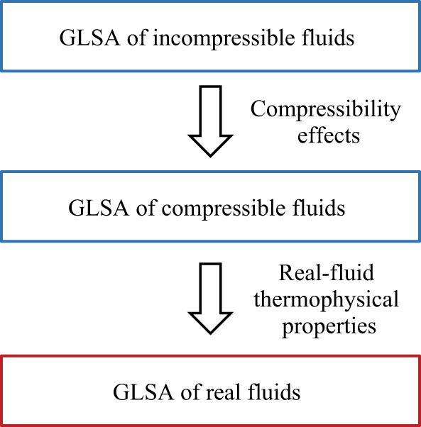

 z/d=0.1
 Rej=2000,R=2

 Ma=0.1
 Re=600
 h=2δ∗


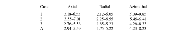

 Q=5×10⁶

 Q=5×10⁶


 w~
 w¯


 St=0.28
 St=0.19
 w~
 Y1¯=0.7


 y

 y
 (uj¯/θ0)2


 St=0.25
 St=0.50
 w~
 Y1~=0.7

 y


 St=0.28
 w~
 Y1¯=0.7

 10

 10


