


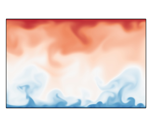



1. Introduction
The investigation of compressible wall-bounded turbulence has always been an important topic and is widely relevant in the aerospace industry. The majority of the early experimental studies have been reviewed by Spina, Smits & Robinson (Reference Spina, Smits and Robinson1994), Bradshaw (Reference Bradshaw1977) and Gatski & Bonnet (Reference Gatski and Bonnet2013). Compared with incompressible wall-bounded turbulence, the compressibility effect has become one of the critical issues, and different Mach numbers and thermal wall boundaries will affect the compressibility of the flow. Morkovin (Reference Morkovin1962) first hypothesized that if density fluctuations are small relative to the mean density, their effect on turbulence is small and can be ignored. This hypothesis is known as Morkovin's hypothesis, and it has led to several compressibility transformations for velocity and Reynolds stresses that aim to map the compressible turbulent statistics onto the ‘equivalent’ incompressible ones using the mean profiles of density and viscosity (Van Driest Reference Van Driest1951; Huang, Coleman & Bradshaw Reference Huang, Coleman and Bradshaw1995; Trettel & Larsson Reference Trettel and Larsson2016; Volpiani et al. Reference Volpiani, Iyer, Pirozzoli and Larsson2020; Griffin, Fu & Moin Reference Griffin, Fu and Moin2021; Hasan et al. Reference Hasan, Larsson, Pirozzoli and Pecnik2023).
As one of the canonical flow problems in compressible wall-bounded turbulence, compressible turbulent channel flows with symmetric isothermal walls have been much studied in past decades since the pioneering work by Coleman, Kim & Moser (Reference Coleman, Kim and Moser1995), who performed direct numerical simulations (DNS) of supersonic turbulent channel flows at Mach number ( $Ma$) 1.5 and 3.0. Here,
 $Ma$ is based on the bulk velocity and sound speed at the wall. They reported that isothermal boundary conditions led to flow that is strongly influenced by wall-normal gradients of mean density and temperature, and these gradients enhanced the streamwise coherence of the near-wall streaks, while almost supporting Morkovin's hypothesis. That is, the turbulent statistics at both Mach numbers agreed well with the corresponding incompressible cases when they were properly scaled. Huang et al. (Reference Huang, Coleman and Bradshaw1995) further analysed the above DNS data, and confirmed that the compressibility effects due to the turbulent density and pressure fluctuations were insignificant. They also found that the strong Reynolds analogy was invalid according to the DNS data, and proposed a more general representation of the analogy. Compressible turbulent channel flows with symmetric isothermal walls were also studied by Foysi, Sarkar & Friedrich (Reference Foysi, Sarkar and Friedrich2004), Wei & Pollard (Reference Wei and Pollard2011), Modesti & Pirozzoli (Reference Modesti and Pirozzoli2016), Gerolymos & Vallet (Reference Gerolymos and Vallet2023), Yu, Xu & Pirozzoli (Reference Yu, Xu and Pirozzoli2019), Tang et al. (Reference Tang, Zhao, Wan and Liu2020), Zhang & Xia (Reference Zhang and Xia2020), Baranwal, Donzis & Bowersox (Reference Baranwal, Donzis and Bowersox2022), Cheng, Shyy & Fu (Reference Cheng, Shyy and Fu2023) and Cheng & Fu (Reference Cheng and Fu2023). Recently, Yao & Hussain (Reference Yao and Hussain2020) carried out a series of DNS of this problem, where
 $Ma=0.8$ and 1.5, and the bulk Reynolds number
 $Re$ was in the range of 3000–34 000. They confirmed that the mean velocity profiles, as well as the Reynolds stress profiles, perfectly collapsed to their corresponding incompressible profiles after the Trettel and Larsson (TL) transformation (Trettel & Larsson Reference Trettel and Larsson2016). Furthermore, their results revealed that the typical eddy size did not vary with
 $Ma$ when scaled using the local friction velocity and thermodynamic properties, and that the compressibility contribution to the skin friction continuously decreases with
 $Re$, suggesting that compressible and incompressible flows differ little when
 $Re$ is high enough. Song et al. (Reference Song, Zhang, Liu and Xia2022) proposed a semi-empirical scaling for the central mean temperature based on the generalized Reynolds analogy (Zhang et al. Reference Zhang, Bi, Hussain and She2014) and available DNS data. Using this empirical scaling, Song, Zhang & Xia (Reference Song, Zhang and Xia2023) proposed a robust iterative method to obtain the mean profiles at given
 $Ma$ and
 $Re$ in compressible turbulent channel flows without performing DNS. More recently, Gerolymos & Vallet (Reference Gerolymos and Vallet2024) performed DNS of compressible turbulent channel flows with symmetric isothermal cold walls across a range of centreline Mach numbers and Reynolds numbers. That study focused on the statistics of the total and static temperature (and enthalpy). The results indicated that the streamwise velocity fluctuations correlate strongly with the total enthalpy fluctuations, while they are not well correlated with the static enthalpy.
In addition to the symmetric isothermal cases, the two walls in compressible turbulent channel flows can also be thermodynamically asymmetric, and understanding the effects of this asymmetry is important to complement the former studies. In general, there are two possible scenarios. One is the case of a temperature difference between two isothermal walls, and the other is the case of an isothermal wall and an adiabatic wall, or the case of isothermal–adiabatic (I–A) walls. The first case has been studied by several groups using DNS or large-eddy simulations, and most of them have focused on the nearly incompressible situations (Wang & Pletcher Reference Wang and Pletcher1996; Lessani & Papalexandris Reference Lessani and Papalexandris2008; Nagata & Nagaoka Reference Nagata and Nagaoka2017; Ma, Yang & Ihme Reference Ma, Yang and Ihme2018; Avellaneda et al. Reference Avellaneda, Bataille, Toutant and Flamant2021), which are believed to be closely related to the flow characteristics in solar receivers (Serra et al. Reference Serra, Toutant, Bataille and Zhou2012; Avellaneda, Bataille & Toutant Reference Avellaneda, Bataille and Toutant2019; Toki, Teramoto & Okamoto Reference Toki, Teramoto and Okamoto2020). For the fully compressible situations with  $Ma>0.3$, studies are rather scarce, and they were carried out mainly to serve as a comparison object for the latter I–A cases (Tamano & Morinishi Reference Tamano and Morinishi2006; Baranwal, Donzis & Bowersox Reference Baranwal, Donzis and Bowersox2023).
In fact, compressible I–A channel flows were first used as a validation case for the B-spline collocation method by Morinishi, Tamano & Nakabayashi (Reference Morinishi, Tamano and Nakabayashi2003). Later on, Morinishi, Tamano & Nakabayashi (Reference Morinishi, Tamano and Nakabayashi2004) carried out a thorough investigation of the effects of adiabatic and isothermal conditions on the turbulent statistics in a compressible I–A channel at  $Ma=1.5$. They reported that Morkovin's hypothesis was not applicable to the near-wall asymptotic behaviour of the wall-normal turbulence intensity, even when the variable property effect was considered. Furthermore, they identified the difference between the energy transfer near isothermal and adiabatic walls by comparing the internal energy and the mean and turbulent kinetic energies.
Tamano & Morinishi (Reference Tamano and Morinishi2006) extended the work of Morinishi et al. (Reference Morinishi, Tamano and Nakabayashi2004), aiming to clarify the effect of thermal wall boundary conditions on turbulence statistics and structures in compressible turbulent channel flows, and to address whether the variations of turbulence statistics are attributable to the effect of the increase in wall temperature caused by the adiabatic wall boundary condition. They simulated a ‘corresponding’ isothermal–pseudo-adiabatic (I–PA) case, where the wall temperature of the upper wall was set to the mean wall temperature of the adiabatic wall, keeping all the other flow parameters the same as those in the I–A case. They reported that the thermal statistics in the I–A case were quite different from those in the corresponding I–PA case. More specifically, they reported that the profiles of mean temperature and root-mean-square (r.m.s.) temperature fluctuations between the I–PA and I–A cases were obviously different, with near-wall maximums appearing near the high-temperature wall for the two profiles in the I–PA case, and that the direction of energy transfer due to pressure work near the adiabatic wall being opposite to that near the isothermal wall is attributable to the effect of the high-temperature wall, not to the effect of the adiabatic wall. However, a subsequent study by Shadloo, Hadjadj & Hussain (Reference Shadloo, Hadjadj and Hussain2015) demonstrated that the basic turbulent statistics in supersonic boundary layers remain unaffected by the thermal boundary conditions between a real adiabatic wall and the corresponding pseudo-adiabatic wall. Zhang et al. (Reference Zhang, Song, Liu and Xia2022) demonstrated that the deviations caused by the three ‘equivalent’ canonical thermal boundary conditions in compressible turbulent channel flows – namely the first boundary condition with fixed wall temperature, the second boundary condition with fixed wall heat flux and the third mixed boundary condition – are limited to the near-wall region. The statistical differences between the I–A case and its corresponding I–PA case from Tamano & Morinishi (Reference Tamano and Morinishi2006) contradict the conclusions drawn by Shadloo et al. (Reference Shadloo, Hadjadj and Hussain2015) and Zhang et al. (Reference Zhang, Song, Liu and Xia2022), which suggested that the cases were nearly equivalent. Therefore, it is necessary to conduct a thorough investigation of the similarities and differences between the two cases.
It is noteworthy that the compressible I–A channel has recently attracted attention. Lusher & Coleman (Reference Lusher and Coleman2022a,Reference Lusher and Colemanb) conducted DNS of turbulent I–A channels at various Mach and Reynolds numbers to investigate the effect of thermal wall conditions on the turbulent Prandtl number ( $Pr_t$) in the low-supersonic regime. They believed that the adiabatic condition was a new feature of particular interest. It was found that
 $Pr_t$ approaches 0.85 away from both the isothermal and the adiabatic walls. The near-wall variations of
 $Pr_t$ collapse as a function of the semi-local wall scaling proposed by Huang et al. (Reference Huang, Coleman and Bradshaw1995), showing only a weak dependence on the wall-friction Reynolds number. Huang et al. (Reference Huang, Coleman, Spalart and Yang2023) further investigated the velocity and temperature scaling near isothermal and adiabatic walls using the data from Lusher & Coleman (Reference Lusher and Coleman2022a). Baranwal et al. (Reference Baranwal, Donzis and Bowersox2023) performed a series of DNS to study the near-wall asymptotic behaviour for the compressible I–A and I–PA cases. That study complemented their earlier research on symmetric isothermal channels (Baranwal et al. Reference Baranwal, Donzis and Bowersox2022). The researchers believed that adiabatic walls could isolate the effects of Mach number from wall cooling, providing a more direct way to assess the effects of Mach number and the validity of Morkovin's hypothesis on the asymptotic scaling of turbulent statistics.
This paper studies supersonic turbulent channel flows with asymmetric thermal walls. The study includes one I–A case and its corresponding I–PA case, as well as two cases with asymmetric isothermal walls of different wall temperature differences. The aim of this study is to clarify the similarities and differences between the I–A case and its corresponding I–PA case, using reliable DNS data to carefully address the conflicts mentioned above. Additionally, we investigate the effect of wall temperature differences between two isothermal walls, especially on the heat transfer behaviour of the channel system with asymmetric wall conditions. The paper is organized as follows. The physical model and numerical set-up are described in § 2. Some basic turbulence statistics are given in § 3. The energy exchange and heat transfer properties are studied in §§ 4 and 5, respectively. Finally, some conclusions are drawn in § 6.
2. Problem description and numerical set-up
In this paper, our main concern is compressible turbulent channel flows between two walls, as depicted in figure 1. The bottom wall is isothermal with fixed wall temperature  $T_L$, whereas the top wall is either adiabatic or isothermal with fixed wall temperature
 $T_{w,t}$. The flow is driven by a uniform force in the streamwise direction. Here,
 $x$,
 $y$ and
 $z$ denote the streamwise, wall-normal and spanwise directions, respectively;
 $x_1$,
 $x_2$ and
 $x_3$ are used interchangeably with
 $x$,
 $y$ and
 $z$. The governing equations are the compressible Navier–Stokes equations, which can be rewritten as follows:
 $$\begin{gather} \frac{\partial \rho}{\partial t}+\frac{\partial \rho u_{j}}{\partial x_{j}}=0, \end{gather}$$
 $$\begin{gather}\frac{\partial \rho u_{i}}{\partial t}+\frac{\partial \rho u_{i} u_{j}}{\partial x_{j}}=-\frac{\partial p}{\partial x_{i}}+\frac{\partial \tau_{i j}}{\partial x_{j}}+f_{i} \delta_{i1}, \end{gather}$$
 $$\begin{gather}\frac{\partial E}{\partial t}+\frac{\partial[u_{i}(E+p)]}{\partial x_{i}}=-\frac{\partial q_{j}}{\partial x_{j}}+\frac{\partial u_{i} \tau_{i j}}{\partial x_{j}}+ f_{1} u_{1}. \end{gather}$$
Here, the Einstein summation convention and notation are used;  $\delta _{ij}$ is the Kronecker tensor,
 $\rho$ the fluid density,
 $u_{i}$ the
 $i$th component of the velocity,
 $p$ the pressure,
 $f_{i}$ the driving volume force and
 $E=\rho (e+u^2_{i}/2)$ the total energy. In the present study, the fluid is assumed to be a perfect gas, and the equation of state
 $p=\rho RT$ is used, where
 $R$ and
 $T$ are the gas constant and temperature, respectively. Here,
 $e=C_vT$ is the internal energy, with
 $C_v=R/(\gamma -1)$ being the specific heat at constant volume, and
 $\gamma =C_{p}/C_{v}$ is the specific heat ratio, with
 $C_{p}$ being the specific heat at constant pressure. The viscous stress
 $\tau _{ij}$ and heat flux
 $q_{j}$ are given as
 \begin{equation} \tau_{i j}=\mu\left(\frac{\partial u_{i}}{\partial x_{j}}+ \frac{\partial u_{j}}{\partial x_{i}} - \frac{2}{3} \frac{\partial u_{k}}{\partial x_{k}} \delta_{i j}\right)\!,\quad q_{j}=-\lambda \frac{\partial T}{\partial x_{j}}, \end{equation}
where  $\mu$, the molecular viscosity, obeys the Sutherland formula and
 $\lambda$, the thermal conductivity, is related to
 $\mu$ through the Prandtl number
 $Pr=C_p\mu /\lambda =0.72$. In what follows, all quantities are non-dimensionalized by the reference temperature
 $T_{ref}=288.15$ K, the channel half-width
 $h$, the bulk density
 $\rho _{m}=\int _{-h}^{h} \bar {\rho }\,{{\rm d}y}/(2h)$ and the bulk velocity
 $u_{m}=\int _{-h}^{h} \overline{\rho u}\,{{\rm d}y}/(2h \rho _m)$ (where
 $\overline {(\,\cdot\,)}$ denotes the Reynolds-averaging operation in the homogeneous directions and time) unless stated otherwise. Besides
 $Pr$, the other two controlling (input) parameters, i.e. the Reynolds number and Mach number,
 \begin{equation} Re=\frac{\rho_{m}u_{m}h}{\mu_{ref}}=6000,\quad Ma=\frac{u_{m}}{\sqrt{\gamma R T_{ref}}}=1.5, \end{equation}
are also fixed unless otherwise stated. Here,  $\mu _{ref}$ is the viscosity at the reference temperature
 $T_{ref}$.
Sketch of compressible turbulent channel flows. The bottom wall is isothermal with  $T_w=T_L$, whereas the top wall is either adiabatic (
 $\partial T/\partial y=0$) or isothermal with wall temperature
 $T_{w,t}$.

In the present study, the simulations are carried out by using the OPENCFD-SC code on a computational box of size  $L_x \times L_y \times L_z =6{\rm \pi} \times 2 \times 4{\rm \pi} /3$. In the OPENCFD-SC code, the inviscid and viscous terms are discretized using a seventh-order upwind scheme and an eighth-order central scheme, respectively, and time is advanced using an explicit third-order Runge–Kutta scheme. The OPENCFD-SC code has been widely employed and validated for compressible turbulent boundary layers (Zhang et al. Reference Zhang, Bi, Hussain and She2014; Liang & Li Reference Liang and Li2015; Li et al. Reference Li, Tong, Yu and Li2019b; Xu et al. Reference Xu, Wang, Wan, Yu, Li and Chen2021) and plane channel flows (Chen & Fei Reference Chen and Fei2018; Yu et al. Reference Yu, Xu and Pirozzoli2019; Zhang & Xia Reference Zhang and Xia2020). The flow is assumed to be periodic in the streamwise and spanwise directions. The boundary conditions for the velocity at both walls are no-slip, whereas the thermal boundaries are different, as mentioned above. The specific control parameters are shown in table 1. The grid is uniform in the streamwise and spanwise directions, and it is clustered in the near-wall region in the wall-normal direction. The detailed grid resolutions are shown in table 2, where the superscript ‘
 $+$’ denotes normalization by using the viscous scale
 $\delta _{v}$ at the nearest wall (also referred to as the wall coordinate). Here,
 $\delta _{v}=\mu _{w} /(\rho _{w} u_{\tau })$ and
 $u_{\tau }=(|\tau_w|/ \rho _{w})^{1/2}$ with
 $\mu _{w}, \rho _{w}$ and
 $\tau _w$ being the viscosity, density and wall shear stress at the nearest wall, respectively. It is found that the current resolutions are comparable to those used by Yao & Hussain (Reference Yao and Hussain2020), Lusher & Coleman (Reference Lusher and Coleman2022a) and Gerolymos & Vallet (Reference Gerolymos and Vallet2023). Figure 2 displays the ratio between the local wall-normal resolution
 $\Delta y$ and the local Kolmogorov scale
 $\eta _k$ in the wall-normal direction for the cases TAd, T25 and T40, demonstrating the sufficiency of the present grid resolutions. Here,
 $\eta _k=(\bar {\rho }\nu ^3/\varepsilon _k)^{1/4}$, with
 $\nu =\bar {\mu }/\bar {\rho }$ being the mean local kinematic viscosity and
 $\varepsilon _k$ the dissipation rate of turbulent kinetic energy (see (4.3) later). It is evident from figure 2(a) that
 $\Delta y/\eta _k$ is less than 1.15 across the channel for the three cases TAd, T25 and T40, indicating that the present mesh resolutions meet the requirement stated by Moin & Mahesh (Reference Moin and Mahesh1998) that the smallest resolved length scale should be
 $O(\eta _k)$. Near the bottom isothermal wall,
 $\Delta z^+\approx 7$–
 $8$, which may be considered slightly coarse for the current simulations. However, as shown in figure 2(b),
 $\Delta z/\delta _v^*$ (see the definition of
 $\delta _v^*$ later) decays rapidly near the bottom wall and remains below 4 for most of the channel (
 $y>-0.9$). We have also refined the grid resolution in the wall-normal and spanwise directions, as well as in the streamwise direction for the TAd case. The results, presented in the Appendix, further confirm the adequacy of the current grid resolutions.
Control parameters and numerical set-up. In all cases,  $Ma=1.5$,
 $Re=6000$,
 $Pr=0.72$ and
 $\gamma =1.4$. The computational domain is
 $L_x \times L_y \times L_z =6{\rm \pi} \times 2 \times 4{\rm \pi} /3$. The temperatures
 $T_{ref}$,
 $T_L$ and
 $T_{w,t}$ are the reference temperature, the wall temperature at the bottom wall and the mean temperature at the top wall, respectively. The parameter
 $N_{t}$ is the number of samples used in the statistics with time interval
 $\Delta t=0.8h/u_m$. The line styles for the four cases are used unless otherwise stated.

Grid resolutions. Here  $Re_\tau =\rho _w u_\tau h/\mu _{w}$ is the friction Reynolds numbers defined using the quantities at the nearest wall, while
 $Re_\tau ^*=\bar {\rho }_c(\tau _w/\bar {\rho }_c)^{1/2} h/\bar {\mu }_c$ is the friction Reynolds number based on the centreline density and viscosity and the friction at the wall;
 $\Delta x$ and
 $\Delta z$ are the grid spaces in the streamwise and spanwise directions;
 $\Delta y_{min}$ and
 $\Delta y_{max}$ denote the wall-normal grid spaces near the wall and at the channel centre. Columns 2–7 display the results normalized by the quantities at the bottom wall (
 $y=-1$), and columns 8–13 show the results at the top wall (
 $y=1$).

(a) The ratio between the local wall-normal resolution  $\Delta y$ and the local Kolmogorov scale
 $\eta _k$ and (b) the ratio between the spanwise resolution
 $\Delta z$ and the semi-local viscous length scale
 $\delta^*_\nu$ in the wall-normal direction for TAd, T25 and T40. The line styles of the cases are as presented in table 1.

The initial velocity fields in the present cases are the laminar parabolic one superimposed with random disturbances, while the density and temperature are uniform. The simulations were initially run on a very coarse mesh and then interpolated to the target fine mesh. Each case was executed using 480 CPU processes for over  $400 h/u_m$ until the flows reached a stationary state. At this point, the turbulent statistics, such as the friction Reynolds numbers at the bottom and top walls, oscillated within a certain range. Then
 $N_t$ samples of the flow fields were stored with a time interval of
 $\Delta t=0.8h/u_m$ for statistical analysis. In the Appendix, a convergence study was conducted, and it was found that most results converged with 100 samples.
In the following, Reynolds decomposition  $(\phi =\bar {\phi }+\phi ^{\prime } \textrm{ with }\bar {\phi }=\langle \phi \rangle )$ and density-weighted Favre decomposition
 $(\phi =\tilde {\phi }+\phi ^{\prime \prime }\textrm{ with }\tilde {\phi }=\overline{\rho \phi } / \bar {\rho }\textrm{ and }\tilde {\phi }=\{\phi \})$ are used, where
 $\langle \phi \rangle =\bar {\phi }$ denotes the averaging operator in the homogeneous spatial directions (
 $x$ and
 $z$) and the temporal direction (
 $t$) by using the
 $N_{t}$ samples of the flow fields. Correspondingly, the r.m.s. value can be defined as
 $\phi _{rms}=(\overline {\phi ^{\prime 2}})^{1/2}$. Furthermore, besides the global coordinate, where
 $y$ is normalized by
 $h$, and the wall coordinate, the semi-local coordinate is also used, where
 $y$ is normalized by the semi-local viscous length scale
 $\delta _{v}^{*}=\bar {\mu } (y) /(\bar {\rho }(y) u_{\tau }^{*})$ with
 $u_{\tau }^{*}=(|\tau_w|/\bar{\rho}(y))^{1 / 2}$ being the semi-local friction velocity. It is obvious that variations of mean density and mean viscosity in the wall-normal direction affect the semi-local coordinate, and its effectiveness has been well documented by many authors (Huang et al. Reference Huang, Coleman and Bradshaw1995; Morinishi et al. Reference Morinishi, Tamano and Nakabayashi2004; Modesti & Pirozzoli Reference Modesti and Pirozzoli2016). Similarly, the friction temperature and the semi-local friction temperature can be defined as
 $T_\tau =q_w /(C_p \rho _w u_\tau )$ and
 $T_\tau ^* =q_w /(C_p \bar {\rho }(y) u_\tau ^*)$, respectively. It is important to note that
 $q_w = 0$ and
 $q_w\approx 0$ for the adiabatic and pseudo-adiabatic walls, respectively. Therefore,
 $T_\tau$ and
 $T_\tau ^*$ are not applicable.
3. Basic turbulence statistics
In compressible turbulence, the velocity and temperature fields are coupled. In turbulent channel flows, it is intuitively expected that the asymmetry of the thermal boundary condition at the two walls will change the symmetry properties of the mean temperature, mean density and mean streamwise velocity. Figure 3 shows profiles of the mean streamwise velocity (normalized by  $u_m$), mean temperature (normalized by
 $T_{ref}$), mean density (normalized by
 $\rho _m$) and local mean Mach number
 $\langle M\rangle =\langle u\rangle (y)/\langle a\rangle (y)$ from TAd, T25, T32 and T40 in global coordinates. It is seen that all the profiles from the four cases are asymmetric about the central plane, i.e.
 $y=0$. Since the thermal boundary conditions at the walls are exerted at the temperature field, the mean temperature profiles from the four cases are clearly asymmetric. The mean temperature first increases rapidly near the bottom wall, and then it increases approximately linearly with
 $y$ in the core region. Near the top wall, the behaviours of the mean temperature are different, depending on the thermal boundary condition there (
 $T_{w,t}/T_L$).
Profiles of (a) the mean streamwise velocity (normalized by  $u_m$), (b) the mean temperature (normalized by
 $T_{ref}$), (c) the mean density (normalized by
 $\rho _m$) and (d) the local mean Mach number
 $\langle M\rangle =\langle u\rangle (y)/\langle a\rangle (y)$ from TAd, T25, T32 and T40 in global coordinates, where
 $\langle a\rangle (y)= \sqrt {\gamma R \langle T\rangle (y)}$ is the local sound speed. The inset in (c) shows a zoomed-in view of the behaviour near the bottom wall.

The mean density in figure 3(c) behaves in a manner inverse to that of the mean temperature. That is, it decreases rapidly near the bottom wall and then decreases slowly further away from the bottom wall. Compared with the mean temperature and density profiles, the mean streamwise velocity profiles, as well as  $\langle M\rangle$, are only slightly asymmetric. When the mean streamwise velocities are normalized by
 $u_m$, the mean profiles are very close to each other in the core region at the fixed
 $Re$ and
 $Ma$, whereas the wall frictions at the two walls show some difference, which can be inferred from the
 $Re_\tau$ values listed in table 2. When the wall friction differences are considered, i.e. the mean velocity is rescaled by using
 $u_\tau$, differences can be observed among TAd (or T32), T25 and T40 in the ‘log-law’ region near both walls, as depicted in figure 4(a,d). It is also seen from these two plots that
 $u^+$ values from the four cases deviate from the incompressible profile near the bottom wall, whereas they are very close to the incompressible one near the top wall.
Mean velocity profiles from the four cases for (a–c) the bottom half and (d–f) the top half: (a,d)  $u^+$ versus
 $y^+$; (b,e)
 $u_{VD}$ versus
 $y^+$; (c,f)
 $U^+$ versus
 $Y^+$. The incompressible DNS results at
 $Re_\tau =180$ (triangles) and 395 (thick grey lines in (a–c)) from Moser, Kim & Mansour (Reference Moser, Kim and Mansour1999) are shown as reference.

In compressible wall-bounded flows, various transformations have been introduced to account for the mean property variations, such as the ‘Van Driest (VD) transformation’ (Van Driest Reference Van Driest1951), where the transformed velocity is
 \begin{equation} u_{VD}=\int_0^{u^+} \left(\frac{\bar{\rho}}{\rho_w}\right)^{1/2}{\rm d} u^+, \end{equation}
and the TL transformation proposed by Trettel & Larsson (Reference Trettel and Larsson2016), where
 $$\begin{gather} Y^{+}=\frac {y} {\delta_v^*}, \end{gather}$$
 $$\begin{gather}U^{+}=\int_{0}^{u^{+}}\left(\frac{\bar{\rho}}{\rho_{w}}\right)^{1 / 2}\left[1+\frac{1}{2} \frac{1}{\bar{\rho}} \frac{{\rm d} \bar{\rho}}{{\rm d}y} y-\frac{1}{\bar{\mu}} \frac{{\rm d} \bar{\mu}}{{\rm d}y} y\right] {\rm d} u^{+}. \end{gather}$$
Trettel & Larsson (Reference Trettel and Larsson2016) summarized the status of the VD transformation and reported that it works very well for adiabatic walls up to  $Ma=20$, while its accuracy deteriorates for increasingly non-adiabatic walls. On the other hand, the TL transformation can produce an excellent collapse of the mean velocity profile at different
 $Re$,
 $Ma$ and wall heat transfer rates. Figure 4(b,c) show the VD-transformed velocity
 $u_{VD}$ versus
 $y+$ and the TL-transformed velocity
 $U^+$ versus
 $Y^+$, respectively, near the bottom wall. The corresponding transformed profiles near the top wall are shown in figure 4(e,f). The incompressible mean velocity profiles in turbulent channel flow at
 $Re_\tau =180$ and 395 (Moser et al. Reference Moser, Kim and Mansour1999) are also shown for reference. As expected, clear deviations between
 $u_{VD}$ and
 $u^+$ (the incompressible DNS data) can be observed at the non-adiabatic bottom wall side. These deviations include a thickened buffer layer and an upward shift of the log-law intercept (Trettel & Larsson Reference Trettel and Larsson2016). The TL-transformed velocities
 $U^+$ from the four cases collapse excellently and match very well with the incompressible DNS data at
 $Re_\tau =395$ in the range
 $Y^+\leq 220$. The top wall is either adiabatic or weakly non-adiabatic in all four cases. As a result, the collapse of
 $u_{VD}$ and
 $U^+$ is successful. These transformed mean velocity behaviours are consistent with the recent findings of Huang et al. (Reference Huang, Coleman, Spalart and Yang2023).
The r.m.s. profiles of the three velocity components can also be studied. If they were normalized by  $u_m$ and shown in the global coordinate, only small deviations between cases T25, T32 (or TAd) and T40 can be observed, mostly near the top wall (not shown for brevity). In compressible turbulent channel flows with symmetric isothermal walls, Coleman et al. (Reference Coleman, Kim and Moser1995) reported that the difference of the r.m.s. velocity fluctuations between the non-zero-Mach-number case and incompressible cases increased with Mach number when normalized by conventional wall variables, whereas the collapse was much better when the semi-local scaling, suggested by Huang et al. (Reference Huang, Coleman and Bradshaw1995), was adopted. Following the studies in Coleman et al. (Reference Coleman, Kim and Moser1995), the r.m.s. profiles of three velocity components in the inner coordinate, normalized by
 $u_\tau$ at the nearest wall, as well as in the semi-local coordinate, normalized by
 $u^*_\tau$ from the nearest wall, from the two halves of the channel are shown in figure 5. In the inner coordinate, as shown in figure 5(a,b), the profiles from the four cases are quite close to each other in the near-wall region with
 $y^+<10$, and are the same for both halves of the channel. For
 $y^+>10$ in the bottom half, the r.m.s. values of the three velocity components are larger for the case with higher
 $T_{w,t}$. The trend is opposite for
 $y^+>10$ in the top half, where the r.m.s. values of the three velocity components are smaller for the case with higher
 $T_{w,t}$. Nevertheless, no obvious difference can be observed for the r.m.s. profiles of the three velocity components between T32 and TAd in both halves, which again shows that the substitution of the adiabatic condition by the pseudo-adiabatic condition will not change the velocity statistics. In the semi-local coordinate, as shown in figure 5(c,d), the deviations between the cases with different
 $T_{w,t}$ become negligible in both halves, illustrating the superiority of the semi-local scaling over the classical wall units in the present problems. It should be noted that the collapsed profiles still deviate from the incompressible ones at
 $Re_\tau =180$ in the bottom half, which is similar to observations in compressible turbulent channels with symmetric isothermal walls (Coleman et al. Reference Coleman, Kim and Moser1995; Modesti & Pirozzoli Reference Modesti and Pirozzoli2016).
Rescaled r.m.s. values of velocity components from the four cases in (a,b) the classical inner coordinate  $y^+$ (normalized by
 $u_\tau$ at the nearest wall) and (c,d) the semi-local coordinate
 $Y^+$ (normalized by
 $u_\tau ^*$) from (a,c) the bottom wall side and (b,d) the top wall side. The incompressible DNS data at
 $Re_\tau =180$ from Moser et al. (Reference Moser, Kim and Mansour1999) (triangles) are shown for comparison.

The superiority of the semi-local scaling over the classical wall units is also valid for the rescaled Reynolds shear stress and streamwise turbulent heat flux, as shown in figure 6, where the Reynolds shear stress near both walls is normalized by  $\tau_w$ at the nearest wall, and in figure 7, where the streamwise turbulent heat flux in the bottom wall side is normalized by
 $\rho _w u_\tau T_\tau =\bar {\rho } u_\tau ^* T_\tau ^*=q_w/C_p$ at the bottom wall. Since
 $q_w=0$ (
 $q_w\approx 0$) at the adiabatic (quasi-adiabatic) wall, the inner/semi-local rescaled streamwise turbulent heat flux in the top half is not shown. From the figures, it is evident that with the semi-local scaling, the collapse behaviours of the Reynolds shear stress and the streamwise turbulent heat flux are much better. For the streamwise turbulent heat flux, although the rescaled ones do not collapse onto each other, their peak locations are almost the same at
 $Y^+\approx 15$.
Reynolds shear stress rescaled by  $\tau _w$ from the four cases in (a,b) the classical inner coordinate
 $y^+$ and (c,d) the semi-local coordinate
 $Y^+$ from (a,c) the bottom wall side and (b,d) the top wall side. The incompressible DNS data at
 $Re_\tau =180$ from Moser et al. (Reference Moser, Kim and Mansour1999) (triangles) are shown for comparison.

Streamwise turbulent heat flux near the bottom wall side rescaled by  $q_w/C_p=\rho _w u_\tau T_\tau =\bar {\rho } u_\tau ^* T_\tau ^*$ at the bottom wall from the four cases in (a) the classical inner coordinate
 $y^+$ and (b) the semi-local coordinate
 $Y^+$.

Now, we turn to the mean temperature profiles again. Following the strategy proposed by Tamano & Morinishi (Reference Tamano and Morinishi2006), the mean temperature  $\bar {T}-T_L$ is rescaled by the temperature difference between the two walls,
 $\Delta T=T_{w,t}-T_L$, and the results from our four cases are shown in figure 8(a). The results of the I–PA case at
 $Ma=1.5$,
 $Re=3000$ and
 $T_{w,t}/T_L \approx 2.4$ from Tamano & Morinishi (Reference Tamano and Morinishi2006) and the I–A case at
 $Ma=1.56$ and
 $Re=6545$ from Lusher & Coleman (Reference Lusher and Coleman2022a) are also shown for comparison. It is evident that the rescaled mean temperature profiles of the present I–A case and the corresponding I–PA case match well with each other, and they also collapse onto the I–A case from Lusher & Coleman (Reference Lusher and Coleman2022a) at similar
 $Re$ and
 $Ma$, demonstrating that the present simulations are reliable, and that the mean temperature differences between the I–A case and the corresponding I–PA case are negligible. The results presented here differ significantly from those reported in Tamano & Morinishi (Reference Tamano and Morinishi2006), where the rescaled mean temperature profiles of their I–A case and the corresponding I–PA case showed a noticeable difference. It is believed that
 $T_{w,t}/T_L$ was underdetermined in the I–A case in Tamano & Morinishi (Reference Tamano and Morinishi2006) due to the simulation not reaching a stationary state, which was understandable given the computational limitations at the time. Lusher & Coleman (Reference Lusher and Coleman2022a) found a significant energy imbalance in Tamano & Morinishi (Reference Tamano and Morinishi2006). Figure 8(a) shows that the rescaled mean temperature profiles from the different cases follow a similar trend in the central bulk region, i.e.
 \begin{equation} \frac{\langle T \rangle-T_L}{\Delta T}= K y + C_{T}. \end{equation}
Here,  $K \approx 0.25$ is the slope of the rescaled mean temperature profile and
 $C_{T}$ is the intercept of the linear temperature profile, which depends on
 $Ma$ and
 $Re$ as well as
 $\Delta T$ (or
 $T_{w,t}$). If we denote by
 $T_A$ and
 $C_{T,A}$ the mean temperature at the adiabatic wall in the I–A case and the corresponding intercept, respectively, then
 $C_{T}>C_{T,A}$ when
 $T_{w,t} < T_A$, and vice versa. Near the top wall, the behaviours of the different cases show diverse trends. For the adiabatic and quasi-adiabatic cases, the mean temperature gradient at the top wall is nearly zero. For the cases with
 $T_{w,t}/T_L<3.234$, i.e. T25 and the case at
 $Ma=1.5, Re=3000 \textrm{ and } T_{w,t}/T_L \approx 2.4$ from Tamano & Morinishi (Reference Tamano and Morinishi2006), the mean temperature gradient at the top wall is negative, that is, the heat will be transferred out from the wall. A local peak of the mean temperature exists near the top wall for these two cases, as was reported in Tamano & Morinishi (Reference Tamano and Morinishi2006), and the peak location is closer to the top wall if
 $T_{w,t}$ is closer to
 $T_A$. For the case with
 $T_{w,t}/T_L>3.234$, i.e. T40, the mean temperature gradient at the top wall is positive, and the heat will be transferred into the fluid through the wall.
(a) Mean temperature profiles rescaled by  $\Delta T=T_{w,t}-T_L$ from the present four cases. The results of the I–PA case at
 $Ma=1.5$,
 $Re=3000$ and
 $T_{w,t}/T_L \approx 2.4$ (circles) from Tamano & Morinishi (Reference Tamano and Morinishi2006) as well as the I–A case at
 $Ma=1.56$ and
 $Re=6545$ (triangles) from Lusher & Coleman (Reference Lusher and Coleman2022a) are also shown. The inset shows a zoomed-in plot near the top wall, and the two dashed vertical lines show the locations of the two local peaks. (b) The r.m.s. profiles of temperature fluctuations from the present four cases (normalized by
 $T_{ref}$). The inset shows a zoomed-in plot near the top wall.

We show in figure 8(b) the r.m.s. profiles of temperature fluctuations from the present four cases. The figure shows clear differences between the three cases, i.e. T25, T32 and T40, and the higher the  $T_{w,t}$, the larger the
 $T_{rms}$ in the bulk region, whereas the deviations between T32 and TAd are negligible except near the top wall, as shown in the inset in figure 8(b), where it allows fluctuation of temperature at the top wall for TAd but does not for T32. In Tamano & Morinishi (Reference Tamano and Morinishi2006), they reported an additional maximum in the region close to the top high-temperature wall, and it was believed to be produced by the maximum of the mean temperature near the high-temperature wall. Nevertheless, there is no extra maximum near the top wall in our results.
Previous studies have shown that in traditional compressible channel flows with symmetric isothermal walls, the mean temperature–velocity relation proposed by Zhang et al. (Reference Zhang, Bi, Hussain and She2014) is effective when the edge location is chosen as the channel centre (Modesti & Pirozzoli Reference Modesti and Pirozzoli2016; Yu et al. Reference Yu, Xu and Pirozzoli2019; Yao & Hussain Reference Yao and Hussain2020). However, this temperature–velocity relation is no longer valid in cases with asymmetric thermal walls, unless the edge location is very close to the walls (not shown here). A direct challenge arises from the asymmetric thermal walls.
4. Energy transfers
In this section, we investigate the energy transfer between the Favre-averaged mean-flow kinetic energy  $\{K_m\}=\{u_{i}\}^{2}/2$, the Favre-averaged turbulent kinetic energy
 $\{k\}=\{u_{i}^{\prime \prime } u_{i}^{\prime \prime }\}/2$ and the Favre-averaged mean internal energy
 $\{e_m\}=C_v \{T\}$ in the four cases. We revise the analyses of Morinishi et al. (Reference Morinishi, Tamano and Nakabayashi2004) and Tamano & Morinishi (Reference Tamano and Morinishi2006) by using our new data to study the three budget equations of
 $\{K_m\}, \{k\}$ and
 $\{e_m\}$.
4.1. Budget equations of  $\{k\}$, $\{K_m\}$ and $\{e_m\}$


The budget equation of turbulent kinetic energy  $\{k\}$ (Huang et al. Reference Huang, Coleman and Bradshaw1995; Morinishi et al. Reference Morinishi, Tamano and Nakabayashi2004) is
 \begin{equation} P_{k}+D_{k}-\varepsilon_{k}+\underbrace{C_{k 1}+C_{k 2}+C_{k 3}}_{C_{k}}=0, \end{equation}
where
 $$\begin{gather} P_{k}=-\overline{\rho u^{\prime \prime} v^{\prime \prime}} \partial \tilde{u} / \partial y, \end{gather}$$
 $$\begin{gather}\varepsilon_{k}=\overline{\tau_{i j}^{\prime} \partial u_{i}^{\prime} / \partial x_{j}}, \end{gather}$$
 $$\begin{gather}D_{k}=\partial\left(\overline{\tau_{i 2}^{\prime} u_{i}^{\prime}}-\overline{p^{\prime} v^{\prime}}-\tfrac{1}{2} \overline{\rho u_{i}^{\prime \prime} u_{i}^{\prime \prime} v^{\prime \prime}}\right) / \partial y, \end{gather}$$
 $$\begin{gather}C_{k1}=-\overline{v^{\prime \prime}} \partial \bar{p} / \partial y,\quad C_{k2}=\overline{u_{i}^{\prime \prime}} \partial \overline{\tau_{i2}} / \partial y,\quad C_{k3}=\overline{p^{\prime} \partial u_{j}^{\prime} / \partial x_{j}}. \end{gather}$$
Here,  $P_{k}$ is the turbulent production term,
 $\varepsilon _{k}$ is the dissipation per unit volume,
 $D_{k}$ is the diffusion term and
 $C_{k}$ is the compressibility term, which is the sum of three terms
 $C_{k1}$,
 $C_{k2}$ and
 $C_{k3}$.
The budget equation of mean-flow kinetic energy  $\{K_m\}$ (Huang et al. Reference Huang, Coleman and Bradshaw1995; Morinishi et al. Reference Morinishi, Tamano and Nakabayashi2004) is
 \begin{equation} D_{K m}-P_{k}-\varepsilon_{K {m}} {-C_{k 1}-C_{k 2}}+P_{K {m}}+f_{K m}=0, \end{equation}
where
 $$\begin{gather} D_{K m}=\partial(\bar{\tau}_{i2}\bar{u}_i-\bar{p} \bar{v}-\overline{\rho u_{i}^{\prime \prime} v^{\prime \prime}} \tilde{u}_{i}) / \partial y, \end{gather}$$
 $$\begin{gather}\varepsilon_{{Km}}=\overline{\tau_{i 2}} \partial \overline{u_{i}} / \partial y, \end{gather}$$
 $$\begin{gather}P_{Km}=\bar{p} \partial \bar{v} / \partial y. \end{gather}$$
Here,  $D_{K m}$ is the mean-flow diffusion term,
 $\varepsilon _{{Km}}$ is the mean-flow dissipation per unit volume,
 $P_{Km}$ is the mean-flow pressure work and
 $f_{Km}$ is the work of the external force.
The budget equation of the mean internal energy  $\{e_m\}$ (Huang et al. Reference Huang, Coleman and Bradshaw1995; Morinishi et al. Reference Morinishi, Tamano and Nakabayashi2004) is
 \begin{equation} D_{em}+\varepsilon_{Km}+\varepsilon_{k}-P_{K m}- C_{k3}=0, \end{equation}
where
 \begin{equation} D_{em}=-\partial(C_{v} \overline{\rho T^{\prime \prime} v^{\prime \prime}}) / \partial y -\partial \overline{q_{2}} / \partial y \end{equation}
is the total diffusion term, including the turbulent diffusion and molecular diffusion. It is easily seen from (4.1), (4.6) and (4.10) that there are seven terms which are responsible for the energy transfers among  $\{k\}$,
 $\{K_m\}$ and
 $\{e_m\}$, and they are
 $P_k$,
 $\varepsilon _{k}$,
 $C_{k1}$,
 $C_{k2}$,
 $C_{k3}$,
 $\varepsilon _{Km}$ and
 $P_{Km}$ (Huang et al. Reference Huang, Coleman and Bradshaw1995; Morinishi et al. Reference Morinishi, Tamano and Nakabayashi2004).
4.2. Energy transfer near both walls
We first study the turbulent kinetic energy budget for the TAd case in the bottom and top halves, and the results are shown in figure 9(a,b), respectively, where the budget terms are normalized by  $\rho _{m} u_{m}^{3}/h$. The balance,
 $P_k-\varepsilon _{k}+D_k+C_k$ (triangles), is almost zero in the whole channel, which confirms that our simulation has reached the fully developed state. From figure 9, it is seen that the dominant terms for
 $\{k\}$ in the near-wall region are
 $P_k$,
 $\varepsilon _k$ and
 $D_k$, while the compressibility term
 $C_k$ is relatively small. The term
 $P_k$ is positive,
 $\varepsilon _k$ is negative, whereas
 $D_k$ is positive in the wall's vicinity and then becomes negative as the wall distance increases until it changes sign again further away from the wall. This scenario is the same for both halves of the channel, although the magnitudes of the terms near the top wall are around half of those near the bottom wall. These observations are consistent with those reported in Morinishi et al. (Reference Morinishi, Tamano and Nakabayashi2004). As a comparison, we also show in figure 9 the corresponding budget terms from the T32 case, and it is evident that the four terms (
 $P_k, -\varepsilon _{k}, D_k, C_k$) match very well with those from the TAd case, again illustrating that the statistics of the turbulent flow field of an I–A case and its corresponding I–PA case are also the same.
Turbulent kinetic energy budget terms (normalized by  $\rho _{m} u_{m}^{3}/h$) in the TAd case near (a) the bottom half and (b) the top half. The corresponding terms from the T32 case are also shown with plus signs.

Morinishi et al. (Reference Morinishi, Tamano and Nakabayashi2004) carefully studied the seven energy exchange/transfer terms and pointed out that the compressibility terms  $C_{k1}$ and
 $C_{k3}$ are negligible close to both the isothermal and the adiabatic walls. In the present study, we have also studied the seven energy exchange/transfer terms in both halves of the channel from the four cases. The wall-normal distributions of
 $P_k$ and
 $-\varepsilon _k$,
 $-\varepsilon _{Km}$ and
 $P_{Km}$, and
 $C_{k2}$ are shown in figures 10–12, respectively. The terms
 $C_{k1}$ and
 $C_{k3}$, which are at least two orders of magnitude smaller than
 $C_{k2}$, are not shown. According to figures 10–12, it is evident that
 $P_k$ is positive while
 $-\varepsilon _k$ and
 $-\varepsilon _{Km}$ are negative in the whole channel for all four cases, indicating that their effects on transferring energy are the same near both the low-temperature and the high-temperature (as well as the adiabatic) walls. On the other hand,
 $P_{Km}$ and
 $C_{k2}$ are obviously negative near the bottom low-temperature wall, whereas they are positive near the top high-temperature wall, illustrating that they behave differently near the low-temperature and high-temperature walls. Near the bottom low-temperature wall,
 $P_{Km}$ transfers energy from
 $\{K_m\}$ to
 $\{e_m\}$, whereas
 $C_{k2}$ transfers kinetic energy from
 $\{k\}$ to
 $\{K_m\}$. Near the top high-temperature wall,
 $P_{Km}$ transfers energy from
 $\{e_m\}$ to
 $\{K_m\}$, whereas
 $C_{k2}$ transfers kinetic energy from
 $\{K_m\}$ to
 $\{k\}$. These observations are the same as those for the I–A case reported in Morinishi et al. (Reference Morinishi, Tamano and Nakabayashi2004). The different values of
 $T_{w,t}$ on the high-temperature wall not only induce obvious deviations (in magnitude) near the high-temperature side, but also can result in some difference near the bottom low-temperature side. Nevertheless,
 $T_{w,t}$ (when it is high enough) will not change the basic behaviour of the energy exchange/transfer among
 $\{K_m\}$,
 $\{k\}$ and
 $\{e_m\}$.
Wall-normal distributions of (a,b)  $P_k$ and (c,d)
 $-\varepsilon _k$ from the four cases. All terms are normalized by
 $\rho _{m} u_{m}^{3}/h$. (a,c) The bottom half; (b,d) the top half. The inset in (a) shows a zoomed-in plot.

Wall-normal distributions of (a,b)  $-\varepsilon _{Km}$ and (c,d)
 $P_{Km}$ from the four cases. All terms are normalized by
 $\rho _{m} u_{m}^{3}/h$. (a,c) The bottom half; (b,d) the top half. The insets in (a,b) show zoomed-in plots.

Wall-normal distributions of  $C_{k2}$ from the four cases. All terms are normalized by
 $\rho _{m} u_{m}^{3}/h$. (a) The bottom half; (b) the top half.

From the above analysis, an intuitive energy exchange/transfer diagram can be constructed, and it is shown in figure 13, where figure 9(a,b) represent the bottom low-temperature side and the top high-temperature side, respectively. The energy exchange terms  $C_{k1}$ and
 $C_{k3}$ are negligible in all four cases when they reach their statistically stationary states. The unidirectional transfer terms
 $P_k$,
 $\varepsilon _k$ and
 $\varepsilon _{Km}$ are the same near both walls, whereas the unidirectional transfer terms
 $P_{Km}$ and
 $C_{k2}$ have opposite transferring directions near the bottom low-temperature side and the top high-temperature side. Furthermore, the four cases have almost the same results, which indicates that the high
 $T_{w,t}$ at the upper wall, whether it is set by the input or induced by the adiabatic wall boundary, is the crucial reason for the changes in the energy transfer direction of
 $P_{Km}$ and
 $C_{k2}$.
Energy exchange/transfer among  $\{k\}$,
 $\{K_m\}$ and
 $\{e_m\}$ near (a) the bottom low-temperature side and (b) the top high-temperature side. A term
 $M$ with
 $A \leftrightarrow B$ means that it mutually exchanges energy between
 $A$ and
 $B$. A term
 $M$ with
 $A\rightarrow B$ means that it transfers energy from
 $A$ to
 $B$, and the directions of the energy transfer are the same near both sides. A term
 $M$ with
 $A\dashrightarrow B$ means that it transfers energy from
 $A$ to
 $B$ and the directions of the energy transfer are opposite near the two sides.

5. Analysis of wall heat transfer
In compressible channels with periodic boundary conditions in wall-parallel directions, the total energy is conserved, and energy exchange occurs on the wall. Many researchers have studied symmetric isothermal channels where there is no temperature difference between the two walls. However, wall heat transfer behaviours in compressible channels with asymmetric thermal wall conditions have not been studied, and this section is devoted to this problem.
5.1. Heat transfer modes in a compressible channel with asymmetric thermal walls
In a compressible channel with asymmetric thermal walls, the heat transfer property of the high-temperature wall depends largely on its wall temperature  $T_{w,t}$, whereas the heat transfer at the low-temperature wall is the same, i.e. transferring heat out of the channel through the wall. This can be easily seen from the mean temperature profiles shown in figures 3(b) and 8. It is evident that there are three kinds of heat transfer modes in such a system. If we denote by
 $T_A$ the mean temperature at the adiabatic wall in an I–A case at prescribed
 $Re$ and
 $Ma$, the three modes can be categorized as the sub-adiabatic, quasi-adiabatic and super-adiabatic modes, respectively, as depicted in figure 14(a–c). For
 $T_L \leq T_{w,t} < T_A$, i.e. the sub-adiabatic mode shown in figure 14(a), there is a peak of the mean temperature profile,
 $T_{max}$, which is located between the channel centre and the top wall while satisfying
 ${\rm d} T/{{\rm d}y}=0$, and heat is transferred out of the fluid system through both walls. A special case is the channel with symmetric isothermal walls, i.e.
 $T_{w,t}=T_L$. In such a situation,
 $T_{max}$ is located at the channel centre according to the symmetry, and an empirical scaling of
 $T_{max}$ was proposed by Song et al. (Reference Song, Zhang, Liu and Xia2022) recently. When
 $T_{w,t}=T_A$, i.e. the quasi-adiabatic mode shown in figure 14(b),
 $T_{max}$ is located at the top wall where
 $q_w\approx 0$ or
 ${\rm d} T/{{\rm d}y}\approx 0$, and no net heat exchange occurs between the top wall and the fluid. Heat can only be transferred out of the fluid system through the bottom wall. When
 $T_{w,t}>T_A$, i.e. the super-adiabatic mode shown in figure 14(c),
 $T_{max}$ is again located at the top wall. However,
 ${\rm d} T/{{\rm d}y}\neq 0$ and heat is transferred to the fluid from the top wall, and it can only be transferred out of the fluid system through the bottom wall. Therefore,
 $T_A$ can be viewed as an important quantity for separating the different heat transfer modes.
Heat transfer modes between the fluid and the walls in a compressible channel with asymmetric thermal walls. (a) Sub-adiabatic state  $T_L \leq T_{w,t} < T_A$ (
 $T_A$ is the mean temperature at the adiabatic wall in the I–A case), where heat is transferred out of the fluid system through both walls. (b) Adiabatic (quasi-adiabatic) state
 $T_{w,t} = T_A$, where heat is transferred out of the fluid system through the bottom wall and almost no net heat exchange occurs between the top wall and the fluid. (c) Super-adiabatic state
 $T_{w,t} >T_A$, where heat is transferred into the fluid system through the top wall and is transferred out of the fluid system through the bottom wall.

5.2. Wall heat flux analysis
Now we investigate the wall heat flux by using integral analysis (Zhang & Xia Reference Zhang and Xia2020; Sun et al. Reference Sun, Guo, Yuan, Zhang, Li and Liu2021; Zhang, Song & Xia Reference Zhang, Song and Xia2021; Wenzel, Gibis & Kloker Reference Wenzel, Gibis and Kloker2022; Xu, Wang & Chen Reference Xu, Wang and Chen2022). In the present study, we start with the internal energy equation (Mittal & Girimaji Reference Mittal and Girimaji2019), and its Reynolds-averaged form can be expressed as (see also (4.10))
 \begin{equation} \frac{\partial}{\partial y}(\bar{q}_{y}+ C_{v} \overline{\rho T^{\prime \prime} v^{\prime \prime}})= \underbrace{-\bar{p} \frac{\partial \bar{v}}{\partial y}-\overline{p^{\prime} \frac{\partial u_{k}^{\prime}}{\partial x_{k}}}}_{\overline{P_{d}}}+ \underbrace{\overline{\tau_{i 2}} \frac{\partial \overline{u_{i}}}{\partial y}+ \overline{\tau_{i j}^{\prime} \frac{\partial u_{i}^{\prime}}{\partial x_{j}}}}_{\overline{V_{a}}}. \end{equation}
Here,  $\overline {P_{d}}=-P_{K m}- C_{k3}$ and
 $\overline {V_{a}}=\varepsilon _{Km}+\varepsilon _{k}$, where the four terms are the energy transfer/exchange terms between
 $\{k\}$ and
 $\{e_m\}$ and between
 $\{K_m\}$ and
 $\{e_m\}$ in § 4. Integrating (5.1) from
 $-1$ to
 $y$, we obtain the heat flux balance at an arbitrary wall-normal location
 $y$:
 \begin{equation} {q}_{w}|_{y=-1}=\bar{q}_y(y)+ C_v\overline{\rho T'' v''}(y) - \int_{-1}^y \overline{P_{{d}}}(y_1) \,{{\rm d}} y_1 -\int_{-1}^y \overline{V_{{a}}}(y_1)\,{\rm d} y_1. \end{equation}
This equation means that the heat transferred into the fluid system through the bottom wall can be estimated through the first law of thermodynamics within the control volume  $[-1, y]$, i.e. the heat transferred out of the control volume through the top boundary at location
 $y$ through the turbulent heat flux
 $C_v\overline {\rho T'' v''}$ and the mean molecular heat flux
 $\bar {q}_y$ subtracts the energy generated inside the control volume through the pressure dilatation work and the viscous stress work. Note that if the value of
 ${q}_w|_{y=-1}$ is negative, the heat is actually transferred out of the fluid system.
Alternatively, we may also integrate (5.1) from  $y$ to
 $1$ to obtain
 \begin{equation} {q}_{w}|_{y=1}=\bar{q}_y(y)+ C_v\overline{\rho T'' v''}(y)+ \int_{y}^1 \overline{P_{{d}}}(y_1)\,{{\rm d}} y_1+\int_{y}^1 \overline{V_{{a}}}(y_1)\,{\rm d} y_1, \end{equation}
which can be physically explained similarly. Considering the special case in (5.2) with  $y=1$, or subtracting (5.3) from (5.2), the total wall heat flux transferred into the fluid system can be obtained:
 \begin{equation} q_{in}={q}_{w}|_{y=-1} - {q}_{w}|_{y=1} =- \int_{-1}^{1} \overline{P_{d}}\,{{\rm d}y} - \int_{-1}^{1} \overline{V_{a}}\,{{\rm d}y}, \end{equation}
or equivalently
 \begin{equation} q_{out}=-q_{in}={q}_{w}|_{y=1} - {q}_{w}|_{y=-1} = \int_{-1}^{1} \overline{P_{d}} \,{{\rm d}y} + \int_{-1}^{1} \overline{V_{a}}\,{{\rm d}y}. \end{equation}
Equation (5.5) indicates that the total heat transfer out of the fluid system through the walls equals the sum of the total pressure dilatation work (the first term on the right-hand side of (5.5)) and the total viscous stress work (the second term on the right-hand side of (5.5)) across the channel. A similar formula was obtained in symmetric compressible turbulent channel flow (Ghosh, Foysi & Friedrich Reference Ghosh, Foysi and Friedrich2010; Zhang et al. Reference Zhang, Song and Xia2021). If we normalize  $q_{in}$ by
 $C_p\rho _wu_\tau T_{ref}$ at the bottom wall, the dimensionless wall heat transfer rate
 $B_q$ can be defined, i.e.
 \begin{equation} B_q= \frac{q_{in}}{C_p \rho_w u_\tau T_{ref}}=\frac{q_{in}}{C_p \rho_w u_\tau T_{L}}. \end{equation}
Correspondingly, the total pressure dilatation work and total viscous stress work contributions of  $B_q$ can be defined as
 $B_{q,P}$ and
 $B_{q,V}$, respectively, according to (5.4). In table 3, we have calculated
 $B_q$ from the four cases based on the temperature gradients on the two walls, i.e. using
 $q_{in}={q_{w}}|_{y=-1} - {q_{w}}|_{y=1}$, as well as that based on the integral analysis, i.e. using the right-hand side of (5.4), and the results strongly suggest that the two estimations match very well with each other, and the relative errors are within 1 %. For the two contribution terms of
 $B_q$ in the integral analysis, i.e.
 $B_{q,P}$ and
 $B_{q,V}$, it is evident from table 3 that the main contribution is
 $B_{q,V}$, for which the contribution exceeds 99.9 % of the total
 $B_q$, and the contribution of
 $B_{q,P}$ is minor, it being around three orders of magnitude smaller than that of
 $B_{q,V}$. This conclusion is consistent with results reported for compressible channels of symmetric isothermal walls by Zhang et al. (Reference Zhang, Song and Xia2021) and physical intuition.
Dimensionless wall heat transfer rate  $B_q$. Here,
 $B_{q,d}$ and
 $B_{q,int}$ are the calculations where
 $q_{in}$ is obtained using
 $q_{in}={q_{w}}|_{y=-1} - {q_{w}}|_{y=1}$ and using the integrals on the right-hand side of (5.4), respectively. The error is defined as
 $(B_{q,d}-B_{q,int})/{B_{q,d}}\times 100\,\%$.

As discussed above, it can be seen from (5.2), (5.3) and (5.4) that  $\bar {q}_y$ and
 $C_v\overline {\rho T'' v''}$ represent the mean heat transfer across the plane
 $y$ from the bottom part to the top part of the channel separated by
 $y$. If the value is negative, the actual heat transfer direction is from the top part to the bottom part. Figure 15 shows the wall-normal distributions of
 $\bar {q}_y$ and
 $C_v\overline {\rho T'' v''}$ from the present four cases. The results from a compressible channel with symmetric isothermal walls at
 $Ma=1.5 \textrm{ and } Re=6000$ from Zhang & Xia (Reference Zhang and Xia2020) are also shown for comparison. For the symmetric isothermal case, it is seen that both terms are zero at the channel centre,
 $y=0$, indicating that there is no mean heat exchange between the top half and the bottom half of the channel, and that the wall heat flux across the wall can be attributed to the work done by the viscous stress and the pressure dilatation. Furthermore,
 $\bar {q}_y$ and
 $C_v\overline {\rho T'' v''}$ are antisymmetric about the channel centre
 $y=0$. In the core region with
 $-0.4 \leq y \leq 0.4$, the heat generated in this region is transferred out mainly through the turbulent heat flux term
 $C_v\overline {\rho T'' v''}$, whereas the mean molecular heat flux term
 $\bar {q}_y$ is approximately zero. In contrast, in the near-wall region with
 $|y| \geq 0.9$,
 $\bar {q}_y$ becomes important and dominates. For the four cases with asymmetric isothermal walls,
 $\bar {q}_y$ and
 $C_v\overline {\rho T'' v''}$ behave very differently, and they are no longer antisymmetric about the channel centre
 $y=0$. For
 $C_v\overline {\rho T'' v''}$, it is negative almost across the channel for all four cases, demonstrating that heat is transferred from the top part down to the bottom part through the plane
 $y$, except that a small region with very small positive values exists very close to the top wall for the T25 case (not shown). For
 $\bar {q}_y$, similar results are obtained. Among the four cases, the smaller
 $T_{w,t}$ is, the larger are the absolute values of
 $\bar {q}_y$ and
 $C_v\overline {\rho T'' v''}$, that is, more heat is transferred from the top part down to the bottom part through the plane
 $y$. Generally,
 $C_v\overline {\rho T'' v''}$ dominates over
 $\bar {q}_y$ except very close to the walls. Nevertheless,
 $B_q$ is smaller since it is defined as the total heat transferred out of the system, which is different from the global-mean heat flux (
 $\langle q_{w}^{ \pm }\rangle =(|\langle q_{y}\rangle |_{y=-1}+|\langle q_{y}\rangle |_{y=1})/2$) defined by Lusher & Coleman (Reference Lusher and Coleman2022a), and there is heat transferred into the system through the top wall if
 $T_{w,t}>T_A$, as discussed in § 5.1.
Wall-normal distributions of (a)  $C_v \overline {\rho T^{\prime \prime } v^{\prime \prime }}$ and (b)
 $\bar {q}_{y}$ from the four cases. The quantities are normalized with
 $C_p \rho _w T_L u_\tau$ at the bottom wall. The results from a compressible channel with symmetric isothermal walls at
 $Ma=1.5 \textrm{ and } Re=6000$ (circles) from Zhang & Xia (Reference Zhang and Xia2020) are also shown for comparison. The inset in (b) shows a zoomed-in plot for
 $-0.8\leq y\leq 0.8$.

From the above analysis, a physical picture emerges: due to the asymmetry of the thermal wall boundary conditions, the symmetry of the heat transfer property breaks. The heat generated by the work done by the pressure dilatation and viscous stress in the top half of the channel will be transferred both upward and downward, separated by the location  $h_0$ where
 $\bar {T}$ reaches its local peak and depends on
 $T_{w,t}$ (see discussions in § 5.1), through
 $\bar {q}_y$ and
 $C_v\overline {\rho T'' v''}$. In the bulk region,
 $C_v\overline {\rho T'' v''}$ plays the dominant role, whereas in the near-wall region
 $\bar {q}_y$ dominates.
5.3. Mathematical relationship between wall heat flux and wall friction
In this section, we derive the relationship between the wall heat flux and the wall friction by using the mean streamwise momentum equation and the mean total energy equation, which are
 \begin{equation} \frac{\partial \overline{\rho u v}}{\partial y}= \frac{\partial \overline{\tau_{12}}}{\partial y}+\bar{f} \end{equation}
and
 \begin{equation} \frac{\partial \overline{E v}}{\partial y}=-\frac{\partial \overline{p v}}{\partial y}+ \frac{\partial \overline{\tau_{i 2} u_{i}}}{\partial y}- \frac{\partial \bar{q}_y}{\partial y}+\overline{u f}, \end{equation}
respectively.
Equations (5.8) and (5.7) are fully integrated from  $-1$ to
 $1$. By using the constraints
 $\int _{-1}^{1} \bar {\rho }\,{{\rm d}y}=2\rho _m$ and
 $\int _{-1}^{1} \overline{\rho u}\,{{\rm d}y}=2\rho _m u_m$ (
 $\rho _m=1$,
 $u_m=1$), we can derive the following equation:
 \begin{equation}
q_{in}={q}_{w}|_{y=-1}-{q}_{w}|_{y=1}=-
({\tau}_{w}|_{y=-1}-{\tau}_{w}|_{y=1})
\frac{\displaystyle\int_{-1}^{1} \bar{u}\,{{\rm d}y}}{2}.
\end{equation}
Equation (5.9) still works for compressible channels with symmetric isothermal walls, and it can also be derived through the overall energy balance, i.e. the heat transferred into the walls equals the total work done by the driving force (Huang et al. Reference Huang, Coleman and Bradshaw1995). With the definition of the skin-friction coefficient  $C_f=2({\tau }_{w}|_{y=-1}-{\tau }_{w}|_{y=1})/(\rho _m u_m^2)$ and
 $U_{avg}=\int _{-1}^{1} \bar {u}\,{{\rm d}y}/2$, we can define the ratio
 $R_{H,F}$, which is similar to the Reynolds analogy factor, as
 \begin{equation} R_{H,F}=-\frac{{B}_q}{C_f}=\frac{\gamma-1}{2}Ma^2 \frac{\rho_m U_{avg}}{\rho_{w}u_\tau}= \frac{\gamma-1}{2}Ma^2\frac{Re}{Re_\tau}\frac{U_{avg}}{u_m}, \end{equation}
where  $Re_\tau$ is the friction Reynolds number at the bottom wall, as listed in table 2. Similarly, if the flow is driven by the external force
 $\rho f$ in the streamwise direction,
 $R_{H,F}$ is slightly modified to
 \begin{equation} R_{H,F}=-\frac{{B}_q}{C_f}=\frac{\gamma-1}{2}Ma^2\frac{\rho_m u_m}{\rho_{w}u_\tau}= \frac{\gamma-1}{2}Ma^2\frac{Re}{Re_\tau}. \end{equation}
A similar relationship was obtained by Li et al. (Reference Li, Fan, Modesti and Cheng2019a) for compressible channels with symmetric isothermal walls. Table 4 presents the directly calculated values of  $C_f$,
 $B_q$,
 $U_{avg}$ and
 $R_{H,F}$ from the present four cases driven by a uniform external force. Here,
 $R_{H,F}$ is estimated using either
 $B_q$ and
 $C_f$ or (5.10). The balance for (5.10) is highly accurate, with relative errors of less than
 $0.8\,\%$, verifying the energy balance in the current simulations. Equation (5.10) also shows that
 $R_{H,F}$ is dependent on
 $Ma$,
 $Re$,
 $Re_\tau$ (at the bottom wall) and the ratio
 $U_{avg}/u_m$, making it a response parameter. For fixed
 $Ma$ and
 $Re$, changing the value of
 $T_{w,t}$ will alter the values of
 $Re_\tau$ at the bottom wall and
 $U_{avg}/u_m$. From the data listed in tables 2 and 4, it can be seen that
 $U_{avg}/u_m$ changes slightly with varying
 $T_{w,t}$, whereas
 $Re_\tau$ at the bottom wall changes greatly. An increase in
 $T_{w,t}$ can lead to an increase in
 $C_f$ (and
 $Re_\tau$ at the bottom wall) and a decrease in
 $B_q$, and therefore a decrease in
 $R_{H,F}$.
Numerical results for the skin-friction coefficient  $C_f$ and wall heat flux coefficient
 $B_q$. The error is defined as
 $(-(B_q / C_f)_d-R_{H,F})/ |(B_q / C_f)_d|\times 100\,\%$ and
 $R_{H,F}$ is defined in (5.10).

6. Conclusions
This paper presents DNS results for compressible turbulent channel flows with asymmetric thermal walls at fixed  $Re=6000$ and
 $Ma=1.5$. The bottom wall is isothermal and fixed at
 $T_L=T_{ref}$, while the top wall is either adiabatic (TAd) or isothermal with
 $T_{w,t}/T_{ref}=2.5$ (T25), 3.234 (T32, the pseudo-adiabatic case) and 4.0 (T40). The study focuses on examining the similarities and differences between the I–A case and its corresponding I–PA case, as well as the effect of the wall temperature difference between the two isothermal walls. It investigates basic turbulent statistics, the heat transfer between the Favre-averaged mean-flow kinetic energy, the Favre-averaged turbulent kinetic energy and the Favre-averaged mean internal energy, as well as wall heat transfer properties. The findings lead to the following conclusions.
(1) Almost all turbulent statistics of the cases TAd and T32 are the same, except for the temperature-fluctuation-related quantities, such as
$T_{rms}$, where some differences can be observed in a small region very close to the top wall. This indicates that the I–A case and its corresponding I–PA case are generally equivalent, and thus the isothermal wall boundary with $T_{w,t}=T_A$ can be used to replace the actual adiabatic boundary condition.(2) The asymmetry of the thermal walls leads to asymmetry of the flow fields and thermal fields. The profiles of mean velocity, r.m.s. of velocity fluctuations and Reynolds shear stress can be well matched in the lower half of the channel in the local semi-local coordinate, but they are less well matched in the upper half of the channel.
(3) In terms of energy transfer behaviour, compared with the energy transfer direction near the bottom wall, the mean-flow pressure work term
$P_{Km}$ and the compressibility term $C_{k2}$ change their transfer direction near the top wall, regardless of whether it is an adiabatic wall or an isothermal wall with high $T_{w,t}$, indicating that the high $T_{w,t}$ at the upper wall is the crucial factor leading to the changes in the energy transfer direction of $P_{Km}$ and $C_{k2}$.(4) By analysing the direction of heat flux on the top high-temperature wall, it is found that
$T_A$ can be used as a criterion to determine the direction of heat flux on the high-temperature sidewall. The turbulent heat flux $C_v\overline {\rho T'' v''}$ and the mean molecular heat flux $\bar {q}_y$ are responsible for the heat transfer generated by the pressure dilatation work and the viscous stress work, where the former dominates in the bulk region and the latter is more important in the near-wall region. The findings have the potential to offer new insights and enhance our understanding of heat transfer phenomena related to wall turbulence prediction and control.


In the future, we will investigate the effects of  $Ma$ and
 $Re$, as well as
 $Pr$, on compressible turbulent channel flows with asymmetric thermal walls. Furthermore, we will try to provide a clear explanation for the linear mean temperature profile in the central bulk region and improve the mean temperature–velocity relation. Additionally, this flow problem has the potential to serve as a complementary canonical test case for assessing the various subgrid-scale models and the Reynolds-averaged Navier–Stokes models.
Acknowledgements
The simulations were carried out on the Hygon C86 7185 GPU processors housed at the Kunshan Computing Center.
Funding
The authors gratefully acknowledge support from the National Natural Science Foundation of China (NSFC grant nos. 92152101 and 92152301).
Declaration of interests
The authors report no conflict of interest.
Appendix. Grid refinement for the TAd case
To demonstrate the adequacy of the grid used in this study, two additional cases were carried out for the TAd case. Grid refinement was performed in the spanwise and wall-normal directions, as well as in the streamwise direction. The detailed grid resolutions in wall units, based on the values at the nearest wall, are presented in table 5. Here, Grid-A ( $864\times 240\times 320$) represents the baseline grid, Grid-B (
 $864\times 400\times 480$) is the spanwise and wall-normal refined grid and Grid-C (
 $1296\times 400\times 480$) is the streamwise, spanwise and wall-normal refined grid. Figure 16 displays a comparison of the mean velocity, mean temperature, mean density and r.m.s. of velocity, temperature and density between the baseline grid (Grid-A) and the refined grids (Grid-B and Grid-C). The statistics demonstrate consistency throughout the entire channel for all three grids. It has been found that the variations of
 $u^*_\tau (y)=\sqrt {|\tau_w|/\bar {\rho }(y)}$ (which are not shown here) along
 $y$ are quite small under the three grid resolutions. Here,
 $\tau _w$ is based on the value at the nearest wall. This illustrates that the three grids have a minimal effect on
 $u_\tau$ and the inner-scaled flow statistics. Additionally, a direct comparison between our TAd case on Grid-A and the aiB case with
 $Re=6545$,
 $Ma=1.56$ and
 $\Delta z^+=6.3$ from Lusher & Coleman (Reference Lusher and Coleman2022a) shows excellent agreement. All the previous discussions have demonstrated that our baseline Grid-A is sufficiently accurate to provide reliable data for the current problem.
Comparisons between three different grids: (a) mean streamwise velocity (normalized by  $u_m$), (b) mean temperature and density (normalized by
 $T_{ref}$ and
 $\rho _m$, respectively), (c) r.m.s. of the three velocity fluctuations (normalized by
 $u_m$) and (d) r.m.s. of temperature and density fluctuations (normalized by
 $T_{ref}$ and
 $\rho _m$, respectively).

Baseline grid resolution (Grid-A:  $864\times 240\times 320$) and refined grid resolutions (Grid-B:
 $864\times 400\times 480$; Grid-C:
 $1296\times 400\times 480$) for the TAd case. The data in columns 2–6 and columns 7–12 are the results normalized by the quantities at the bottom wall (
 $y=-1$) and top wall (
 $y=1$), respectively.



