


1 Introduction
The general position problem in graph theory was independently introduced (at least) three times, which clearly demonstrates that the concept is of wide interest. The first time, it was investigated in the context of hypercubes [Reference Körner7] and later extended to the general case [Reference Manuel and Klavžar9, Reference Ullas Chandran and Jaya Parthasarathy18]. The latter article has led to extensive research on the problem, and a recent review article [Reference Ullas Chandran, Klavžar and Tuite19] lists 126 references. The study of general position sets has extended to various types, such as Steiner position sets [Reference Klavžar, Kuziak, Peterin and Yero6], edge general position sets [Reference Manuel, Prabha and Klavžar10], mutual-visibility sets [Reference Di Stefano2], mobile position sets [Reference Klavžar, Krishnakumar, Tuite and Yero5], monophonic position sets [Reference Thomas, Ullas Chandran, Tuite and Di Stefano13], vertex position sets [Reference Thankachy, Ullas Chandran, Tuite, Thomas, Di Stefano and Erskine12] and lower general position sets [Reference Di Stefano, Klavžar, Krishnakumar, Tuite and Yero3]. Among the recent achievements in the field, we would like to highlight [Reference Araujo, Dourado, Protti and Sampaio1, Reference Iršič, Klavžar, Rus and Tuite4, Reference Thomas, Ullas Chandran, Tuite and Di Stefano14–Reference Tuite, Thomas and Ullas Chandran17].
We now define the problem. If
 $G = (V(G), E(G))$
is a simple, connected graph, then the set
 $X\subseteq V(G)$
is a general position set for the graph G if for every two vertices
 $v,u\in X$
and every shortest
 $(u,v)$
-path P, no inner vertex of P lies in X. We are interested in the size of a largest general position set of G which is called the general position number of G and denoted by
 $\mathrm {gp}(G)$
.
The General Position Set problem for a given graph G and a positive integer
 $k\leq |V(G)|$
asks whether there exists a general position set S for G such that
 $|S|\geq k$
. It was already shown in the seminal paper [Reference Manuel and Klavžar9] that the General Position Set problem is NP-complete for arbitrary graphs. The closely related Lower General Position problem was proved to be NP-complete in [Reference Di Stefano, Klavžar, Krishnakumar, Tuite and Yero3], and the Monophonic Position Set problem was demonstrated to be NP-hard in [Reference Thomas, Ullas Chandran, Tuite and Di Stefano13]. Interestingly, it is not clear whether the Monophonic Position Set problem is NP-complete for general graphs.
Since determining the general position number of a graph is difficult in general, it is reasonable to approach it in different algorithmic ways. Korže and Vesel [Reference Korže and Vesel8] described a reduction from the problem of finding a general position set in a graph to the satisfiability problem and applied the approach to the case of general position sets of hypercubes. However, we are not aware of any systematic algorithmic approach to the General Position Problem. Therefore, in this note, we propose three different algorithms for approaching the problem. These approaches are integer linear programming (ILP), genetic algorithm (GA) and simulated annealing (SA), and are described in the next section. In Section 3, these approaches are tested on several large graphs from different areas of graph theory.
2 Three approaches
In this section, we present in respective subsections the three approaches to compute the general position number as announced in the introduction.
2.1 Integer linear programming model
Let G be a graph with vertex set
 $V(G) = \{v_1,\ldots , v_{n(G)}\}$
, where
 $n(G)$
denotes the order of G. To find a general position set of G with the maximum cardinality, for a given set
 $X\subseteq V(G)$
, define binary variables
 $x_j$
,
 $j\in [n(G)]$
, which constitute a characteristic vector of X, that is,
 $$ \begin{align*} x_j = \begin{cases} 1 & \mbox{if } v_j \in X, \\ 0 & \text{otherwise}. \end{cases} \end{align*} $$
Then, the objective function is to maximise
 $\sum _{j = 1}^{n} x_j$
. For each two vertices
 $v_i$
and
 $v_j$
, let
 $I_G(v_i,v_j)$
be the set of vertices different from
 $v_i$
and
 $v_j$
which lie on at least one shortest
 $(v_i,v_j)$
-path. Therefore, if
 $v_i, v_j\in X$
, that is, if
 $x_i + x_j = 2$
, then we must have
 $\sum _{x_\ell \in I_G(v_i , v_j)} x_\ell = 0$
, which can be considered as the inequality:
 $$ \begin{align*} \sum_{x_\ell \in I(v_i , v_j)}x_\ell \le 0. \end{align*} $$
Using integer modelling techniques, we model this constraint as
 $$ \begin{align*} \sum_{v_\ell \in I(v_i , v_j)}x_\ell + M(x_i + x_j-1) \leq M, \quad i,j \in [n(G)], \end{align*} $$
where M is an upper bound for the constraint
 $\sum _{v_\ell \in I(v_i , v_j)}x_\ell \leqslant 0$
. In this case, we can select
 $M = n(G)$
. The ILP for our problem is thus:
 $$\begin{align*}\max \sum_{j = 1}^{n} x_j \end{align*}$$
such that
 $$\begin{align*}\sum_{v_\ell \in I(v_i , v_j)}x_\ell + n(G)(x_i + x_j) \leq 2n(G), \quad i,j \in [n(G)], \ x_i \in \{0,1\}, \ i\in [n(G)]. \end{align*}$$
2.2 Genetic algorithm
In this subsection, we present a Genetic Algorithm (GA for short) to find the largest general position sets. GA is a population-based method and is well suited for the general position problem because it efficiently explores large search spaces while maintaining feasible solutions through its crossover and mutation operators.
Before implementing the GA, it is necessary to define the stopping criterion, the fitness function and the genetic operators specific to this problem. Each instance of a solution S for a graph G is represented as a binary (characteristic) vector of size
 $n(G)$
, that is, if the vertex i is included in the solution, then
 $S(i)=1$
, otherwise,
 $S(i)=0$
. The stopping criterion is defined as the maximum number of iterations. The objective of the algorithm is to obtain a solution that satisfies the general position constraints while maximising the number of selected vertices. The fitness function for a solution S is defined as
 $$ \begin{align*} \mathrm{Fitness}(S) = \sum S - M \cdot f, \end{align*} $$
where
 $\sum S$
represents the total number of selected vertices and f denotes the number of violations of the general position condition. Specifically, for every pair of vertices u and v with
 $S(u) = 1$
and
 $S(v) = 1$
, if there exists a vertex w on a shortest
 $(u,v)$
-path with
 $S(w) = 1$
, then f is increased. The penalty term
 $M \cdot f$
ensures that solutions violating the general position condition are penalised proportionally to the number of violations, where M is a large constant balancing the trade-off between maximising the number of selected vertices and maintaining feasibility. The initial population is generated randomly, ensuring diversity in the search space.
For parent selection, we use a random selection method. The offspring generation process involves combining two parent solutions: the new solution instance is a binary vector, where a vertex is included if it appears in at least one of the parents.
The mutation operator selects two vertices randomly and swaps their values.
The GA presented in Algorithm 1 outlines the general structure of the approach for solving the general position problem, in terms of the various operators which have been explained above.

2.3 Simulated annealing
Simulated Annealing (SA for short) is a single-solution point-based metaheuristic algorithm inspired by the annealing process in metallurgy. Before implementing SA for the general position problem, it is essential to define the stopping criterion, the neighbourhood generation mechanism and the fitness function. The algorithm begins with an initial solution
 $S_0$
, which is a vector of zeros and ones representing the inclusion or exclusion of vertices in the solution set. The quality of a solution is measured by the fitness function,
 $\mathrm {Fitness}(S)$
, which is defined in the same way as for the GA.
The acceptance probability of a new solution is determined by the Metropolis criterion, which depends on the current temperature and the change in the objective value. The temperature gradually decreases according to a predefined cooling schedule. In our implementation of the Simulated Annealing algorithm, we employed a geometric cooling schedule, where the temperature is updated as
 $$ \begin{align*} T_{k+1}\leftarrow T_k*\rho, \end{align*} $$
where
 $\rho $
is the cooling rate and we start with an initial temperature,
 $T_0$
. The algorithm terminates once the maximum number of iterations or a minimum temperature is reached.
The SA is formally presented in Algorithm 2.
3 Experimental results
We have performed our experiments on sets of examples. The first examples come from mathematical chemistry, the second examples deal with hypercubes, while the last examples come from algebraic graph theory. The implementation code for the algorithms is available upon request from the authors.

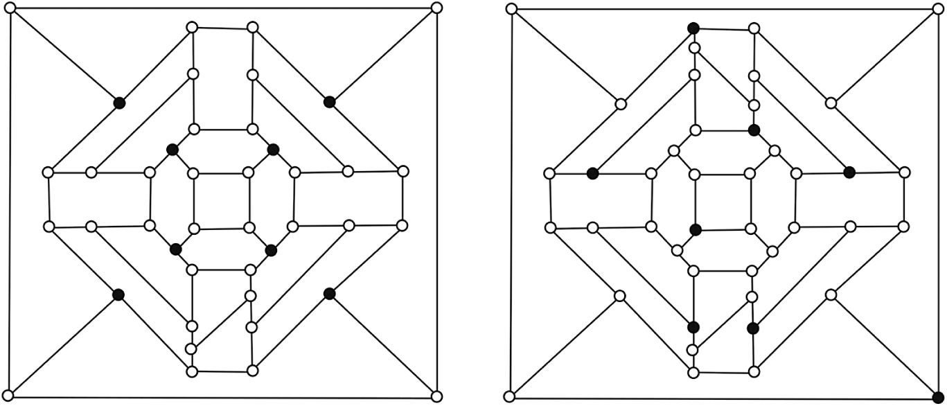
Maximum general position sets for
 $C_{42}$
and
 $C_{44}$
.

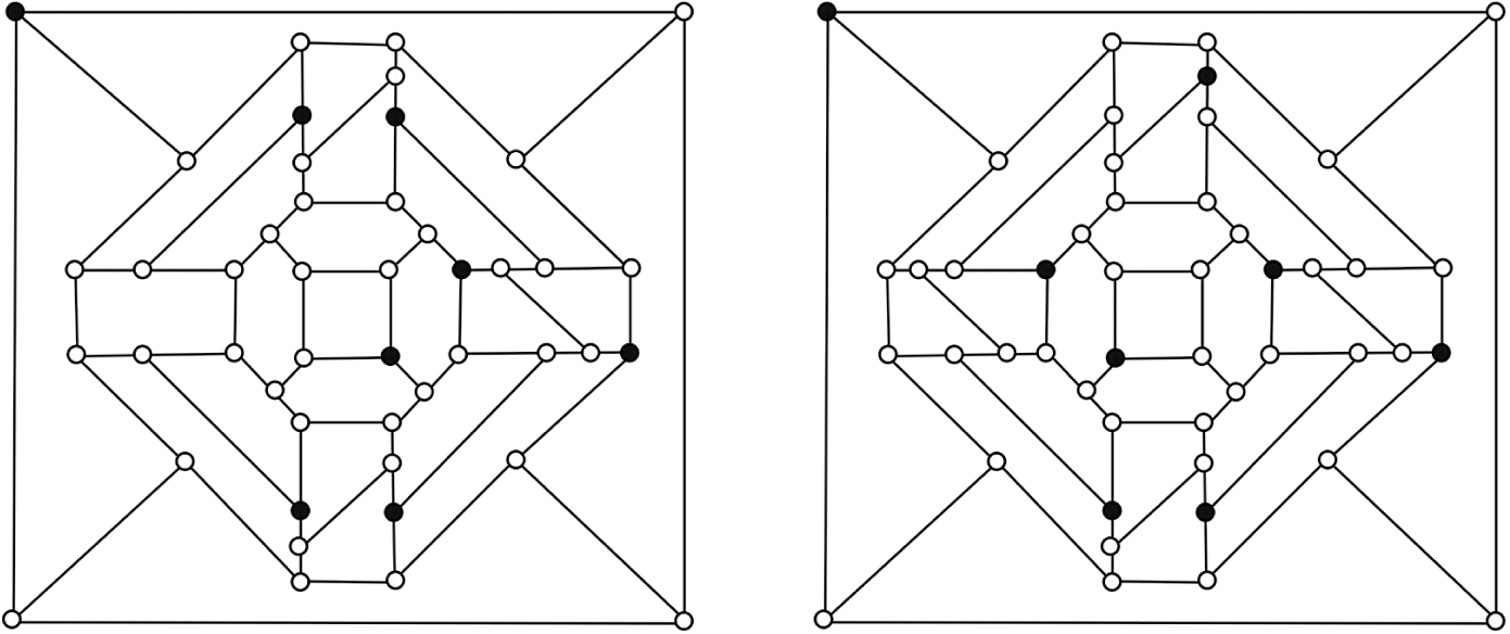
Maximum general position sets for
 $C_{46}$
and
 $C_{48}$
.

From the area of chemical graph theory, we have considered the so-called middle-fullerene graphs
 $C_{42}$
,
 $C_{44}$
,
 $C_{46}$
and
 $C_{48}$
from [Reference Melker and Krupina11] (see Figures 1 and 2).
The maximum general position sets of
 $C_{42}$
and
 $C_{44}$
, as indicated in Figure 1 with solid dots, were obtained by solving the corresponding ILP model. In the case of the middle-fullerene graphs
 $C_{46}$
and
 $C_{48}$
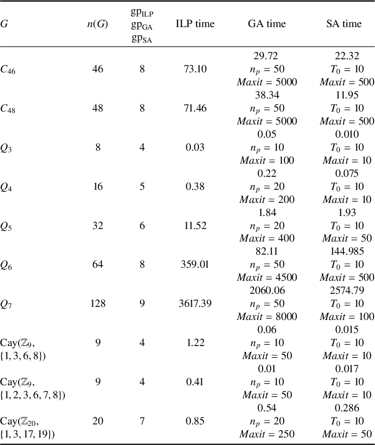
, their examination was carried out using all three algorithms. The results are reported in the top two rows of Table 1 and the concrete largest general position sets obtained can be seen in Figure 2.
The general position number of some graphs and running times of the ILP, GA and SA.

Let
 $Q_n$
denote the n-dimensional hypercube. It is known ever since [Reference Körner7] that it is intrinsically difficult to determine
 $\mathrm {gp}(Q_n)$
in general. The small values
 $\mathrm {gp}(Q_1) = \mathrm {gp}(Q_2) = 2$
and
 $\mathrm {gp}(Q_3) = 4$
can be determined by hand, while the values
 $\mathrm {gp}(Q_4) = 5$
,
 $\mathrm {gp}(Q_5) = 6$
,
 $\mathrm {gp}(Q_6) = 8$
and
 $\mathrm {gp}(Q_7) = 9$
were reported in [Reference Korže and Vesel8, Table 1]. In this note, we have verified these values by our three algorithms. The computational results are presented in the middle of Table 1.
For the last set of examples, we have considered three examples from algebraic graph theory, the Cayley graphs
 $\mathrm {Cay}(\mathbb {Z}_9,\{1,3,6,8\})$
,
 $\mathrm {Cay}(\mathbb {Z}_9,\{1,2,3,6,7,8\})$
and
 $\mathrm {Cay}(\mathbb {Z}_{20},\{1,3,17,19\})$
. The computational results are summarised in the last three rows of Table 1.
As can be seen from Table 1, SA was the fastest in six cases and GA in four cases. Both algorithms generally seem to be faster than ILP, which has never been the fastest.
4 Conclusion and future directions
In this paper, we have proposed and implemented two meta-heuristic algorithms, Genetic Algorithm (GA) and Simulated Annealing (SA), to tackle the general position problem. While both methods show promising results for various graphs, there is potential for exploring other meta-heuristic approaches that offer a comparable trade-off between solution quality and computation time. For instance, algorithms such as Ant Colony Optimisation or Particle Swarm Optimisation may enhance the search capabilities, especially when coupled with high-performance computing resources. These approaches could be particularly useful for instances where even linear programming models fail due to the size and complexity of the input graph.