2. The Mathieu equations

We consider a cylindrical container filled with three Newtonian fluids of different densities, as depicted in figure 1(a). The motion of the three-layer fluid is governed by the Navier–Stokes equation

(2.1)\begin{equation} \rho_j \left (\frac{\partial \boldsymbol{V}_j}{t} + \boldsymbol{V}_j \boldsymbol{\cdot} \boldsymbol{\nabla} \boldsymbol{V}_j \right)=-\boldsymbol{\nabla} P_j + \mu_j\,\nabla^2 \boldsymbol{V}_j-\rho_j \left[ g + a_c \cos 2\omega t \right] \boldsymbol{e}_z, \end{equation}

and the continuity equation

(2.2)\begin{equation} \boldsymbol{\nabla}\boldsymbol{\cdot} \boldsymbol{V}_j = 0, \end{equation}

where $\boldsymbol {V}_j=u_j \boldsymbol {e}_x+v_j \boldsymbol {e}_y+w_j \boldsymbol {e}_z$, $P_j$, $\mu _j$ and $\rho _j$ are the velocity, pressure, kinetic viscosity and density of corresponding fluid $j$. Here, the subscript $j = 1, 2, 3$ denotes the liquid at the bottom, middle and top, respectively; $g$ denotes the acceleration due to gravity, while $a_c$ stands for the acceleration amplitude provided by the vibrator. In general, the vibration acceleration satisfies the formula $a_c = 4A \omega ^2$, where $A$ is the vibrational amplitude.

According to linear stability analysis, the solution of the ideal fluid equations (2.1)–(2.2) can be expanded in an asymptotic series as $\boldsymbol {V}_j=\boldsymbol {V}^{\prime }_j$, $P_j=P_{0,j}+P^{\prime }_j$. Therefore, the base state domain equations and the perturbation equations can be written as

(2.3)$$\begin{gather} \frac{\partial{P_{0,j}}}{\partial{z}}=-\rho_j \left(g+4A\omega^2 \cos\varOmega t\right), \end{gather}$$

(2.4)$$\begin{gather}\rho_j\,\frac{\partial{\boldsymbol{V}^{\prime}_{j}}}{\partial{t}}=-\boldsymbol{\nabla} P^{\prime}_j+\mu_j\,\nabla^2\boldsymbol{V}^{\prime}_j. \end{gather}$$

2.1. The inviscid model

Considering the ideal fluids, the non-rotating flow, and the stress-free sidewall assumption, similar to the Benjamin derivation process (Benjamin & Ursell Reference Benjamin and Ursell1954), we can get the $z$-direction velocity $w_j$ to satisfy the Helmholtz equation

(2.5)\begin{equation} \left( \frac{\partial^2}{\partial z^2}-k^2 \right) w_j=0, \end{equation}

where $k$ is the wavenumber in the horizontal plane. For cylindrical containers, $k=k_{ln}$ is the $n$th zero of ${\rm J}'_l(k_{ln}R)$, where ${\rm J}_l$ is a Bessel function of $l$th order. Equation (2.5) has a general solution

(2.6)\begin{equation} w_j=A_j(t)\mathrm{cosh}\,kz+B_j(t)\mathrm{sinh}\,kz. \end{equation}

At the wall, the no-penetration conditions are

(2.7)\begin{equation} \left.\begin{gathered} w_1=0 \quad \mathrm{at} \ z=0,\\ w_3=0 \quad \mathrm{at} \ z=h_1+h_2+h_3. \end{gathered}\right\}\end{equation}

At interface $A$, the flow satisfies the conditions

(2.8)$$\begin{gather} w_1=w_2=\frac{\mathrm{d}\xi_A}{\mathrm{d}t}, \end{gather}$$

(2.9)$$\begin{gather}\rho_2\,\frac{\partial}{\partial z}\frac{\partial w_2}{\partial t}-\rho_1\,\frac{\partial}{\partial z}\frac{\partial w_1}{\partial t} =-\left[ \left(\rho_2-\rho_1 \right)\left( g-a_c \cos 2\omega t\right)-\sigma_A k^2 \right]k^2 \xi_A. \end{gather}$$

At interface $B$, the flow satisfies the conditions

(2.10)$$\begin{gather} w_2=w_3=\frac{\mathrm{d}\xi_B}{\mathrm{d}t}, \end{gather}$$

(2.11)$$\begin{gather}\rho_3\,\frac{\partial}{\partial z}\frac{\partial w_3}{\partial t}-\rho_2\,\frac{\partial}{\partial z}\frac{\partial w_2}{\partial t} =-\left[ \left(\rho_3-\rho_2 \right)\left( g-a_c \cos 2\omega t\right)-\sigma_B k^2 \right]k^2 \xi_B. \end{gather}$$

From (2.6)–(2.11), the Mathieu equations of a three-layer inviscid fluid are obtained as

(2.12)$$\begin{gather} \frac{\mathrm{d}^2 \xi_A}{\mathrm{d} t^2}-\beta_A\,\frac{\mathrm{d}^2 \xi_B}{\mathrm{d} t^2} + \varOmega^2_A \left(1+F_A \cos 2\omega t\right) \xi_A = 0, \end{gather}$$

(2.13)$$\begin{gather}\frac{\mathrm{d}^2 \xi_B}{\mathrm{d} t^2}-\beta_B\,\frac{\mathrm{d}^2 \xi_A}{\mathrm{d} t^2} + \varOmega^2_B \left(1+F_B \cos 2\omega t\right) \xi_B = 0, \end{gather}$$

where $\varOmega _A$ and $\varOmega _B$ are natural frequencies of the interfaces $A$ and $B$:

(2.14a,b)\begin{equation} \varOmega^2_A=\frac{(\rho_1-\rho_2)gk+\sigma_A k^3}{\rho_1\,\mathrm{coth}\, kh_1+\rho_2\,\mathrm{coth}\,kh_2},\quad \varOmega^2_B=\frac{(\rho_2-\rho_3)gk+\sigma_B k^3}{\rho_2\,\mathrm{coth} \,kh_2+\rho_3\,\mathrm{coth}\,kh_3}. \end{equation}

In addition, other parameters are

(2.15a,b)$$\begin{gather} F_A = \frac{\left(\rho_1-\rho_2\right)a_c}{\sigma_A k^2+\left(\rho_1-\rho_2\right)g},\quad F_B = \frac{\left(\rho_2-\rho_3\right)a_c}{\sigma_B k^2+\left(\rho_2-\rho_3\right)g}, \end{gather}$$

(2.16a,b)$$\begin{gather}\beta_A = \frac{\rho_2/\mathrm{sinh}\,kh_2}{\rho_1\,\mathrm{coth}\,kh_1+\rho_2\,\mathrm{coth}\,kh_2},\quad \beta_B = \frac{\rho_2/\mathrm{sinh}\,kh_2}{\rho_2\,\mathrm{coth}\,kh_2+\rho_3\,\mathrm{coth}\,kh_3}, \end{gather}$$

where subscripts $A$ and $B$ represent the interfaces $A$ and $B$, respectively. Here, $F_A$ and $F_B$ describe the relative magnitudes of vibration acceleration, and $\beta _A$ and $\beta _B$ describe the strength of coupling between interfaces.

We then derive the Mathieu equations of an $N$-layer fluid model (figure 2) for the inviscid fluids by adopting a method similar to that for the three-layer fluid model, and present the details in Appendix A.

Figure 2.

Schematic diagram of $N$-layer fluid system.

The following simplified equations (2.17), (2.18) can be obtained easily from (2.12), (2.13) under the assumption that $kh_2\gg 1$:

(2.17)$$\begin{gather} \frac{\mathrm{d}^2\xi_A}{\mathrm{d}t^2}+\varOmega^2_A\left( 1+F_A \cos 2\omega t \right)\xi_A=0, \end{gather}$$

(2.18)$$\begin{gather}\frac{\mathrm{d}^2\xi_B}{\mathrm{d}t^2}+\varOmega^2_B\left( 1+F_B \cos 2\omega t \right)\xi_B=0. \end{gather}$$

In this case, the equations are decoupled into two two-layer inviscid models, indicating that there is no coupling between the motions of the two interfaces when the thickness of the medium-density fluid is large enough. It is consistent with the results from Ward et al. (Reference Ward, Zoueshtiagh and Narayanan2019b).

2.2. The viscous model

While inviscid models can explain partially the mechanism of Faraday waves, they cannot provide the acceleration threshold due to the neglect of viscous dissipation. Landau & Lifshitz (Reference Landau and Lifshitz1987) presented a method to calculate the rate of viscous dissipation by estimating the energy of viscous dissipation. The Faraday wave of a two-layer fluid is extended further and compared with Floquet's model (Kumar & Tuckerman Reference Kumar and Tuckerman1994), showing good agreement. This study proposes a simplification in a three-layer viscous model (Labrador et al. Reference Labrador, Sánchez, Porter and Shevtsova2021). The Mathieu equations of a three-layer viscous fluid can be obtained by considering only the direct viscous action of fluids on both sides of the interface:

(2.19)$$\begin{gather} \frac{\mathrm{d}^2\xi_A}{\mathrm{d}t^2}-\beta_A\,\frac{\mathrm{d}^2\xi_B}{\mathrm{d}t^2}+2\gamma_A\, \frac{\mathrm{d}\xi_A}{\mathrm{d}t}+\varOmega^2_A\left( 1+F_A\cos 2\omega t\right)\xi_A=0, \end{gather}$$

(2.20)$$\begin{gather}\frac{\mathrm{d}^2\xi_B}{\mathrm{d}t^2}-\beta_B\,\frac{\mathrm{d}^2\xi_A}{\mathrm{d}t^2}+2\gamma_B\, \frac{\mathrm{d}\xi_B}{\mathrm{d}t}+\varOmega^2_B\left( 1+F_B\cos 2\omega t\right)\xi_B=0, \end{gather}$$

where $\gamma _A$ and $\gamma _B$ are the damping coefficients of the interfaces $A$ and $B$,

(2.21a,b)\begin{align} \gamma_A = \frac{2k^2\left( \mu_1\,\mathrm{coth}\,kh_1+\mu_2 \,\mathrm{coth}\,kh_2\right)}{\rho_1\,\mathrm{coth}\,kh_1+\rho_2\,\mathrm{coth}\,kh_2},\quad \gamma_B = \frac{2k^2\left( \mu_2\,\mathrm{coth}\,kh_2+\mu_3 \,\mathrm{coth}\,kh_3\right)}{\rho_2\,\mathrm{coth}\,kh_2+\rho_3\,\mathrm{coth}\,kh_3}. \end{align}

Applying the Faraday instability in microgravity, the viscous model ((2.19) and (2.20)) is validated by the simulations from Labrador et al. (Reference Labrador, Sánchez, Porter and Shevtsova2021). We can estimate these damping coefficients through an evaluation of viscous dissipation energy. The longer the wavelength, the more significant the viscous damping (Batson et al. Reference Batson, Zoueshtiagh and Narayanan2013) of the interface and the wall boundary layer becomes. When the wavenumber is large, viscous damping arises primarily from internal damping, which can be estimated by calculating the dissipated viscous energy (Herreman et al. Reference Herreman, Nore, Guermond, Cappanera, Weber and Horstmann2019; Kumar & Tuckerman Reference Kumar and Tuckerman1994).

On the basis of (A7), we add the viscous correction term to get the Mathieu equations of an $n$-layer viscous fluid:

(2.22)\begin{equation} \begin{cases} \dfrac{\text{d}^2\xi_1}{\text{d}t^2}-\beta_{1,2}\,\dfrac{\text{d}^2\xi_2}{\text{d}t^2}+2\gamma_1\, \dfrac{\mathrm{d}\xi_1}{\mathrm{d}t}+\varOmega_1\left( 1+F_1\cos 2\omega t \right)\xi_1 =0,\\[9pt] \vdots\\[4pt] \dfrac{\text{d}^2\xi_i}{\text{d}t^2}-\beta_{i,i-1}\,\dfrac{\text{d}^2\xi_{i-1}}{\text{d}t^2}-\rho_{i,i+1}\,\dfrac{\text{d}^2\xi_{i+1}}{\text{d}t^2}+2\gamma_i\, \dfrac{\mathrm{d}\xi_i}{\mathrm{d}t}+\varOmega_i\left( 1+F_i\cos 2\omega t \right)\xi_i =0, \\[9pt] \quad 1< i< N-1,\\[3pt] \vdots\\[4pt] \dfrac{\text{d}^2\xi_{N-1}}{\text{d}t^2}-\beta_{N-1,N-2}\,\dfrac{\text{d}^2\xi_{N-2}}{\text{d}t^2}+2\gamma_{N-1}\, \dfrac{\mathrm{d}\xi_{N-1}}{\mathrm{d}t}+\varOmega_{N-1}\left( 1+F_{N-1}\cos 2\omega t \right)\xi_{N-1} =0, \end{cases} \end{equation}

where

(2.23)\begin{equation} \gamma_i=\frac{2k^2\left( \mu_i \,\mathrm{coth}\,kh_i+\mu_{i+1} \,\mathrm{coth}\,kh_{i+1} \right)}{\rho_i \,\mathrm{coth}\,kh_i+\rho_{i+1} \,\mathrm{coth}\,kh_{i+1}}. \end{equation}

3. Floquet analysis

Floquet analysis can be applied to parametric instability problems such as Faraday waves. Ward et al. (Reference Ward, Zoueshtiagh and Narayanan2019b) performed a Floquet analysis of the three-layer Faraday waves on the Kumar theoretical model (Kumar & Tuckerman Reference Kumar and Tuckerman1994; Kumar Reference Kumar1996), and found that Floquet analysis can be generalized to three-layer fluid systems. In the same way, we carried out Floquet analysis on the Mathieu equations (2.19) of a three-layer viscous fluid.

The Floquet expansion is used to separate the variables

(3.1)\begin{equation} \left.\begin{gathered} \xi_A = {\rm e}^{{\rm i} kx} \sum_{n=-\infty }^{\infty } {\rm e}^{q_n t}\,\hat{\xi} _{A,n},\\ \xi_B = {\rm e}^{{\rm i} kx} \sum_{n=-\infty }^{\infty } {\rm e}^{q_n t}\,\hat{\xi} _{B,n}, \end{gathered}\right\} \end{equation}

where $q_n=s+\mathrm {i}( \alpha +n)2\omega$. The stability curves for harmonic ($\alpha = 0$) and subharmonic ($\alpha = 1/2$) solutions can be obtained by setting $s=0$, where $s$ is the growth rate. Substitute (3.1) into (2.19)–(2.20) to get

(3.2)\begin{equation} \left.\begin{gathered} \left( q^2_n+2q_n \gamma_A+\varOmega^2_A\right)\hat{\xi}_{A,n}-\beta_A q^2_n\, \hat{\xi}_{B,n}+\frac{\varOmega^2_A F_A}{2} \left( \hat{\xi}_{A,n-1}+\hat{\xi}_{A,n+1}\right)=0,\\ \left( q^2_n+2q_n \gamma_B+\varOmega^2_B\right)\hat{\xi}_{B,n}-\beta_B q^2_n\, \hat{\xi}_{A,n}+\frac{\varOmega^2_B F_B}{2} \left( \hat{\xi}_{B,n-1}+\hat{\xi}_{B,n+1}\right)=0. \end{gathered}\right\} \end{equation}

These equations can be formulated as an eigenvalue problem for $\hat {\xi }_{A,n}, \hat {\xi }_{B,n}$, where $A$ is the eigenvalue. The eigenvalue equation is

(3.3)\begin{equation} \begin{pmatrix} q^2_n+2q_n\gamma_A+\varOmega^2_A & -\beta_A q^2_n \\ -\beta_B q^2_n & q^2_n+2q_n\gamma_B+\varOmega^2_B \end{pmatrix} \begin{pmatrix} \hat{\xi}_{A,n} \\ \hat{\xi}_{B,n} \end{pmatrix} = A\omega^2 \begin{pmatrix} \chi_A & 0 \\ 0 & \chi_B \end{pmatrix} \begin{pmatrix} \hat{\xi}_{A,n-1}+\hat{\xi}_{A,n+1} \\ \hat{\xi}_{B,n-1}+\hat{\xi}_{B,n+1} \end{pmatrix}\!, \end{equation}

where

(3.4a,b)\begin{equation} \chi_A =-\frac{\varOmega^2_A}{2}\,\frac{\rho_1-\rho_2}{\sigma_A k^2+( \rho_1-\rho_2)g},\quad \chi_B =-\frac{\varOmega^2_B}{2}\,\frac{\rho_2-\rho_3}{\sigma_B k^2+( \rho_2-\rho_3)g}. \end{equation}

Further, we can write (3.3) as a system of linear equations

(3.5)\begin{equation} \boldsymbol{M} \begin{pmatrix} \hat{\xi}_A \\ \hat{\xi}_B \end{pmatrix} = A \omega^2 \begin{pmatrix} \chi_A \boldsymbol{C} & 0 \\ 0 & \chi_B \boldsymbol{C} \end{pmatrix} \begin{pmatrix} \hat{\xi}_A \\ \hat{\xi}_B \end{pmatrix}, \end{equation}

where $\hat {\xi }_A,\hat {\xi }_B$ are column vectors

(3.6a,b)\begin{equation} \hat{\xi}_A=\begin{pmatrix} \hat{\xi}_{A,-n} \\ \hat{\xi}_{A,-n+1} \\ \vdots \\ \hat{\xi}_{A,0} \\ \vdots \\ \hat{\xi}_{A,n-1} \\ \hat{\xi}_{A,n} \end{pmatrix},\quad \hat{\xi}_B=\begin{pmatrix} \hat{\xi}_{B,-n} \\ \hat{\xi}_{B,-n+1} \\ \vdots \\ \hat{\xi}_{B,0} \\ \vdots \\ \hat{\xi}_{B,n-1} \\ \hat{\xi}_{B,n} \end{pmatrix}, \end{equation}

and $\boldsymbol {M}$ and $\boldsymbol {C}$ are banded matrices

(3.7)\begin{gather} \boldsymbol{M} = \begin{pmatrix}\begin{smallmatrix} q^2_{-n}+2q_{-n}\gamma_A+\varOmega^2_A & & & & & & -\beta_A q^2_{-n} & & & & & \\ & & & \ddots & & & & & & \ddots & & \\ & & & & & q^2_n+2q_n\gamma_A+\varOmega^2_A & & & & & & -\beta_A q^2_n\\ -\beta_B q^2_{-n} & & & & & & q^2_{-n}+2q_{-n}\gamma_B+\varOmega^2_B & & & & & \\ & & & \ddots & & & & & & \ddots & & \\ & & & & & -\beta_B q^2_n & & & & & & q^2_n+2q_n\gamma_B+\varOmega^2_B \end{smallmatrix}\end{pmatrix}, \end{gather}

(3.8)\begin{gather} \boldsymbol{C} = \begin{pmatrix} 0 & 1 & & & & \\ 1 & 0 & 1 & & & \\ & 1 & 0 & 1 & & \\ & & 1 & 0 & 1 & \\ & & & 1 & 0 & 1 \\ & & & & 1 & 0 \end{pmatrix}. \end{gather}

The stability boundaries are defined by the curves in the $A\unicode{x2013} k$ plane on which $s(A, k)=0$, for a certain frequency $\omega$. Note that the eigenvalue $A$ must be a positive real number.

4. Asymptotic analysis

To facilitate the solution, the dimensionless Mathieu equations of a three-layer viscous fluid (2.19)–(2.20) are obtained, where the time scale is $1/\omega$:

(4.1)$$\begin{gather} \ddot{\xi}_A - \beta_A \ddot{\xi}_B + 2\hat{\mu}_A \dot{\xi}_A + \left( \delta_A + \hat{\varepsilon}_A \cos 2t \right)\xi_A=0, \end{gather}$$

(4.2)$$\begin{gather}\ddot{\xi}_B - \beta_B \ddot{\xi}_A + 2\hat{\mu}_B \dot{\xi}_B + \left( \delta_B + \hat{\varepsilon}_B \cos 2t \right)\xi_B=0, \end{gather}$$

where $\hat {\mu }_A = \gamma _A/\omega$, $\hat {\mu }_B = \gamma _B/\omega$, $\delta _A = \varOmega ^2_A/\omega ^2$, $\delta _B = \varOmega ^2_B/\omega ^2$, $\hat {\varepsilon }_A = F_A\varOmega ^2_A/\omega ^2$ and $\hat {\varepsilon }_B = F_B\varOmega ^2_B/\omega ^2$.

Let a small quantity of the system be $\epsilon = a_c/g$. It is also assumed that $\hat {\mu }_A$ and $\hat {\mu }_B$ are of order $O ( \epsilon )$ for a low-viscosity fluid system. Then $\hat {\mu }_A=\epsilon \mu _A$, $\hat {\mu }_B=\epsilon \mu _B$, $\hat {\varepsilon }_A=\epsilon \varepsilon _A$ and $\hat {\varepsilon }_B=\epsilon \varepsilon _B$. Physically, $\epsilon$ is the dimensionless amplitude of externally excited acceleration. This treatment method is based on the work of Rajchenbach & Clamond (Reference Rajchenbach and Clamond2015). Asymptotically expand $\xi _A$, $\xi _B$, $\delta _A$ and $\delta _B$, as

(4.3)\begin{equation} \left.\begin{gathered} \xi_A=\xi_{A0}+\epsilon \xi_{A1}+\epsilon^2 \xi_{A2}+O (\epsilon^3), \\ \xi_B=\xi_{B0}+\epsilon \xi_{B1}+\epsilon^2 \xi_{B2}+O (\epsilon^3), \\ \delta_A=\delta_{A0}+\epsilon \delta_{A1}+\epsilon^2 \delta_{A2}+O (\epsilon^3), \\ \delta_B=\delta_{B0}+\epsilon \delta_{B1}+\epsilon^2 \delta_{B2}+O (\epsilon^3). \end{gathered}\right\} \end{equation}

According to the characteristics of Faraday waves, at order $O (\epsilon ^0)$, the natural frequency of the fluid system is about half of the excitation frequency, that is, $\omega \approx \omega _0$, where $\omega _0$ is the natural frequency of the fluid system. Therefore, we define $\delta _{A0} = \varOmega _A ^ 2 / \omega _0 ^ 2$ and $\delta _{B0} = \varOmega _B ^ 2 / \omega _0 ^ 2$.

By substituting (4.3) into (4.1)–(4.2), it is easy to get the zero-order approximation equations (4.4), the first-order approximation equations (4.5), and the second-order approximation equations (4.6):

(4.4)\begin{gather} \left.\begin{gathered} \ddot{\xi}_{A0}-\beta_A \ddot{\xi}_{B0} +\delta_{A0} \xi_{A0} = 0,\\ \ddot{\xi}_{B0}-\beta_B \ddot{\xi}_{A0} +\delta_{B0} \xi_{B0} = 0.\end{gathered}\right\} \end{gather}

(4.5)\begin{gather} \left.\begin{gathered} \ddot{\xi}_{A1}-\beta_A \ddot{\xi}_{B1} +\delta_{A0} \xi_{A1} =-2\mu_A \dot{\xi}_{A0}-\left( \delta_{A1}+ \varepsilon_A \cos 2t \right)\xi_{A0},\\ \ddot{\xi}_{B1}-\beta_B \ddot{\xi}_{A1} +\delta_{B0} \xi_{B1} =-2\mu_B \dot{\xi}_{B0}-\left( \delta_{B1}+ \varepsilon_B \cos 2t \right)\xi_{B0}. \end{gathered}\right\} \end{gather}

(4.6)\begin{gather} \left.\begin{gathered} \ddot{\xi}_{A2}-\beta_A \ddot{\xi}_{B2} +\delta_{A0} \xi_{A2} =-2\mu_A \dot{\xi}_{A1}-\delta_{A2}\xi_{A0}- \left( \delta_{A1}+ \varepsilon_A \cos 2t \right)\xi_{A1},\\ \ddot{\xi}_{B2}-\beta_B \ddot{\xi}_{A2} +\delta_{B0} \xi_{B2} =-2\mu_B \dot{\xi}_{B1}-\delta_{B2}\xi_{B0}-\left( \delta_{B1}+ \varepsilon_B \cos 2t \right)\xi_{B1}. \end{gathered}\right\} \end{gather}

The solution of (4.4) can be written in the form

(4.7)\begin{equation} \left.\begin{gathered} \xi_{A0} = A_0\cos t+B_0\sin t,\\ \xi_{B0} = C_0\cos t+D_0\sin t, \end{gathered}\right\} \end{equation}

where $A_0$, $B_0$, $C_0$, $D_0$ are all undetermined coefficients. Substitute (4.7) into (4.4) to derive the subsequent equations

(4.8a)$$\begin{gather} \begin{pmatrix} \delta_{A0}-1 & \beta_A\\ \beta_B & \delta_{B0}-1 \end{pmatrix} \begin{pmatrix}{A_0}\\ {C_0}\end{pmatrix} =0, \end{gather}$$

(4.8b)$$\begin{gather}\begin{pmatrix} \delta_{A0}-1 & \beta_A\\ \beta_B & \delta_{B0}-1 \end{pmatrix} \begin{pmatrix}{B_0}\\ {D_0}\end{pmatrix} =0. \end{gather}$$

Since the undetermined coefficients ($A_0, B_0, C_0, D_0$) cannot be equal to 0, which implies the existence of a non-zero solution, the determinant of the coefficient matrix must be 0:

(4.9)\begin{equation} \begin{vmatrix} \delta_{A0}-1 & \beta_A \\ \beta_B & \delta_{B0}-1 \end{vmatrix} =0. \end{equation}

Equation (4.9) can also be written as

(4.10)\begin{equation} \begin{vmatrix} \dfrac{\varOmega_A ^ 2}{\omega_0^ 2} -1 & \beta_A \\[10pt] \beta_B & \dfrac{\varOmega_B ^ 2}{\omega_0^2}-1 \end{vmatrix} =0. \end{equation}

In this case, $\omega _0$ satisfies

(4.11)\begin{equation} \beta_A\beta_B=\frac{\left( \omega^2_0-\varOmega^2_A \right)\left( \omega^2_0-\varOmega^2_B \right)}{\omega^4_0}, \end{equation}

where $\omega _{0,1}$ and $\omega _{0,2}$ ($\omega _{0,1}>\omega _{0,2}$) are the two non-negative roots of the equation.

Substitute (4.7) into (4.5) to get

(4.12) \begin{align} \ddot{\xi}_{A1}-\beta_A \ddot{\xi}_{B1}+\delta_{A0}\xi_{A1} &= \frac{1}{2}\left(-2A_0\delta_{A1}-A_0\varepsilon_A-4B_0\mu_A\right)\cos t\nonumber\\ &\quad +\frac{1}{2}\left(-2B_0\delta_{A1}+B_0\varepsilon_A+4A_0\mu_A \right)\sin t\nonumber\\ &\quad +\frac{1}{2}\left(-A_0 \varepsilon_A \cos 3t-B_0\varepsilon_A\sin 3t \right), \end{align}

(4.13)\begin{align} \ddot{\xi}_{B1}-\beta_B \ddot{\xi}_{A1}+\delta_{B0}\xi_{B1} &= \frac{1}{2}\left(-2C_0\delta_{B1}-C_0\varepsilon_B-4D_0\mu_B\right)\cos t \nonumber\\ &\quad +\frac{1}{2}\left(-2D_0\delta_{B1}+D_0\varepsilon_B+4C_0\mu_B \right)\sin t\nonumber\\ &\quad +\frac{1}{2}\left(-C_0 \varepsilon_B \cos 3t-D_0\varepsilon_B\sin 3t \right). \end{align}

The secular terms in (4.12) and (4.13) are eliminated to obtain

(4.14a,b)\begin{equation} \delta_{A1}={\pm}\sqrt{\frac{\varepsilon^2_A}{4}-4\mu^2_A},\quad \delta_{B1}={\pm}\sqrt{\frac{\varepsilon^2_B}{4}-4\mu^2_B}, \end{equation}

and

(4.15)\begin{equation} \left.\begin{gathered} \xi_{A1}=\frac{A_0\varepsilon_A\left(\delta_{B0}-9\right)-9C_0\beta_A\varepsilon_B}{162 \beta_A \beta_B-2\left(\delta_{A0}-9\right)\left(\delta_{B0}-9\right)}\cos 3t + \frac{B_0\varepsilon_A\left(\delta_{B0}-9\right)-9D_0\beta_A\varepsilon_B}{162 \beta_A \beta_B-2\left(\delta_{A0}-9\right)\left(\delta_{B0}-9\right)}\sin 3t,\\ \xi_{B1}=\frac{C_0\varepsilon_B\left(\delta_{A0}-9\right)-9A_0\beta_B\varepsilon_A}{162 \beta_A \beta_B-2\left(\delta_{A0}-9\right)\left(\delta_{B0}-9\right)}\cos 3t + \frac{D_0\varepsilon_B\left(\delta_{A0}-9\right)-9B_0\beta_B\varepsilon_B}{162 \beta_A \beta_B-2\left(\delta_{A0}-9\right)\left(\delta_{B0}-9\right)}\sin 3t. \end{gathered}\right\} \end{equation}

In the same way, the secular terms of (4.6) are eliminated to obtain

(4.16)\begin{equation} \left.\begin{gathered} \delta_{A2} = \frac{\varepsilon_A\left(\left(\delta_{A0}-1\right)\left(\delta_{B0}-9\right)\varepsilon_A+9\beta_A^2\varepsilon_B\right)}{4\left(\delta_{A0}-1\right)\left(\left(\delta_{A0}-9\right)\left(\delta_{B0}-9\right)-81\beta_A\beta_B\right)},\\ \delta_{B2} = \frac{\varepsilon_B\left(\left(\delta_{A0}-9\right)\left(\delta_{B0}-1\right)\varepsilon_B+9\beta_B^2\varepsilon_A\right)}{4\left(\delta_{B0}-1\right)\left(\left(\delta_{A0}-9\right)\left(\delta_{B0}-9\right)-81\beta_A\beta_B\right)}. \end{gathered}\right\} \end{equation}

From (4.14a,b) and (4.16), the second-order approximate solutions for $\delta _A$ and $\delta _B$ are obtained as

(4.17)\begin{equation} \left.\begin{gathered} \delta_A = \frac{\varOmega^2_A}{\omega^2_0}\pm\sqrt{\frac{\hat{\varepsilon}^2_A}{4}-4\mu^2_A}+ \frac{\hat{\varepsilon}_A\left(\left(\delta_{A0}-1\right)\left(\delta_{B0}-9\right) \hat{\varepsilon}_A+9\beta_A^2\hat{\varepsilon}_B\right)}{4\left(\delta_{A0}-1\right) \left(\left(\delta_{A0}-9\right)\left(\delta_{B0}-9\right)-81\beta_A\beta_B\right)},\\ \delta_B = \frac{\varOmega^2_B}{\omega^2_0}\pm\sqrt{\frac{\hat{\varepsilon}^2_B}{4}- 4\mu^2_B}+\frac{\hat{\varepsilon}_B\left(\left(\delta_{A0}-9\right)\left(\delta_{B0}-1\right) \hat{\varepsilon}_B+9\beta_B^2\hat{\varepsilon}_A\right)}{4\left(\delta_{B0}-1\right) \left(\left(\delta_{A0}-9\right)\left(\delta_{B0}-9\right)-81\beta_A\beta_B\right)}. \end{gathered}\right\} \end{equation}

It can be seen that the interface coupling effect exists not only in the dispersion relation (4.11), but also in the second-order term of acceleration (4.17). However, viscosity is one of the factors to inhibit Faraday instability at both multi-fluid and single-fluid interfaces.

Furthermore, (4.14a,b) can be written in terms of variations of $\omega$:

(4.18)\begin{equation} \left( 1-\frac{\omega^2}{\omega_0^2} \right) \approx \frac{F_A^2}{4} - \frac{4\gamma_A^2 \omega^2}{\varOmega_A^4}=O\left( \epsilon \right) \end{equation}

and

(4.19)\begin{equation} \left( 1-\frac{\omega^2}{\omega_0^2} \right) \approx \frac{F_B^2}{4} - \frac{4\gamma_B^2 \omega^2}{\varOmega_B^4}=O\left( \epsilon \right). \end{equation}

So when $\omega \approx \omega _0$ is satisfied, critical instability occurs. From (4.14a,b), we can obtain

(4.20a,b)\begin{equation} F_A=\frac{4\gamma_A}{\varOmega^2_A}\omega_0,\quad F_B=\frac{4\gamma_B}{\varOmega^2_B}\omega_0. \end{equation}

Further, (4.20a,b) is dimensionalized to get

(4.21)\begin{equation} \left.\begin{gathered} a_{cA}=8k\omega\,\frac{\mu_1\,\mathrm{coth}\,kh_1+\mu_2\,\mathrm{coth}\,kh_2}{\rho_1-\rho_2},\\ a_{cB}=8k\omega\,\frac{\mu_2\,\mathrm{coth}\,kh_2+\mu_3\,\mathrm{coth}\,kh_3}{\rho_2-\rho_3}, \end{gathered}\right\} \end{equation}

where $a_{cA}$ and $a_{cB}$ correspond to the critical excitation accelerations of two subharmonic instability modes (discussed in detail in § 6), respectively. To facilitate the comparison with the experimental results, the vibration amplitude (4.22) is derived:

(4.22a)$$\begin{gather} A_{cA}=\frac{2k}{\omega}\,\frac{\mu_1\,\mathrm{coth}\,kh_1+\mu_2\,\mathrm{coth}\,kh_2}{\rho_1-\rho_2}, \end{gather}$$

(4.22b)$$\begin{gather}A_{cB}=\frac{2k}{\omega}\,\frac{\mu_2\,\mathrm{coth}\,kh_2+\mu_3\,\mathrm{coth}\,kh_3}{\rho_2-\rho_3} . \end{gather}$$

It is worth noting that when $kh_2\gg 1$ (i.e. the middle fluid is thick enough), a result identical to that of the single interface is obtained:

(4.23a,b)\begin{equation} \omega_{0,A}=\varOmega_A,\quad \omega_{0,B}=\varOmega_B \end{equation}

and

(4.24)\begin{equation} \left.\begin{gathered} \delta_A = \frac{\varOmega^2_A}{\omega^2_0}\pm\sqrt{\frac{\hat{\varepsilon}^2_A}{4}-4\mu^2_A}+\frac{\hat{\varepsilon}_A^2}{4 (\delta_{A0}-9)}, \\ \delta_B = \frac{\varOmega^2_B}{\omega^2_0}\pm\sqrt{\frac{\hat{\varepsilon}^2_B}{4}-4\mu^2_B}+\frac{\hat{\varepsilon}_B^2}{4 (\delta_{B0}-9)}. \end{gathered}\right\} \end{equation}

Equations (4.23a,b)–(4.24) are the solution for interfaces $A$ and $B$. In this case, the double interface is completely decoupled, and the fluctuations do not interfere with each other.

5. Experimental systems and measurement methods

The schematic diagram of the double-interface fluid system is shown in figure 3. A cylindrical tank of inner diameter 55 mm is mounted on a vertical vibration system that consists of an SA-JZ020 electromagnetic shaker, an FY6900 function generator and an HEA-500G power amplifier. With the help of the CDAQ-9171 data acquisition system, the acceleration of the tank measured by the SAE D0005B accelerometer can be stored with a high sample rate. A homemade Python code is adopted to realize a combined operation of the vertical vibration system, the data acquisition system and the high-speed camera system (Phantom VEO 340S).

Figure 3.

Schematic diagram of the experimental system.

We select eutectic alloy GaInSn (66.7 % Ga, 20.5 % In, 12.5 % Sn), which is in a liquid state at room temperature, as the working fluid. We place 30 ml (${h_1=12.62\ \textrm {mm}}$) GaInSn in the cylindrical container, and then add 3 ml (${h_2=1.262\ \textrm {mm}}$) sodium hydroxide solution ($1\ \textrm {mol}\ \textrm {l}^{-1}$) on the surface of the GaInSn to prevent oxidizing. Here, it is important to note that although the oxide surface layer can be removed by both acidic and alkaline solutions, we have chosen to use a $1\ \textrm {mol}\ \textrm {l}^{-1}$ concentration of sodium hydroxide due to its milder chemical reaction (Handschuh-Wang et al. Reference Handschuh-Wang, Chen, Zhu and Zhou2018). The interfacial tension coefficients $\sigma _A$ between the GaInSn and the sodium hydroxide solution, and $\sigma _B$ between the sodium hydroxide solution and air, are obtained by the pendant drop method. The OCA25 contact angle measuring instrument (manufactured in Germany) measures the interfacial tension coefficient with resolution $0.01\ \textrm {mN}\ \textrm {m}^{-1}$. Since the air density is much smaller than in the GaInSn and sodium hydroxide solution, we consider only the physical properties of the GaInSn and sodium hydroxide solution that are listed in table 1.

Table 1.

The fluid properties.

A high-speed camera is mounted directly above the container to capture the shape of the interface with the help of LED lights on the side of the container through a semi-transparent and semi-reflective mirror. Regarding the two fluid interfaces present in the system, it is difficult to distinguish each interface accurately when the fluids are transparent, as in Ward et al. (Reference Ward, Zoueshtiagh and Narayanan2019b) while studying the Faraday wave in three-layer fluid systems. In the present study, however, the situation is quite different. The reflectance of the GaInSn/solution interface is much stronger than that of the solution/air interface, and as a result, the camera captures most of the reflected light from the GaInSn/solution interface and less from the solution/air interface. Since the camera's optical axis is parallel to the reflected light, the bright areas correspond to the antinodes of the wave, while the dark areas correspond to the nodes. The magnitude of the brightness is determined by the slopes of the surface waves, with darker regions having larger slopes as shown in figure 4. This allows the modal pattern of the GaInSn/solution interface surface waves to be acquired by overhead recording, reflecting the spatial distribution of the surface waves. Moreover, in the present experimental system, two interfaces are coupled strongly to each other and exhibit synchronous fluctuations.

Figure 4.

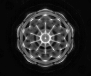
(a–c) Theoretical prediction of surface shapes of mode $(n, l)$. (d–f) Surface shapes plotted by one minus absolute value. (g–i) Faraday patterns. The driving frequency of the vibrator is $f$, which satisfies $\varOmega =2{\rm \pi} f$, where $n$ and $l$ are the radial and azimuthal mode numbers.

Due to the wetting properties, a meniscus is formed at the interface between the GaInSn and the sodium hydroxide solution, curving towards the GaInSn side. Similarly, at the interface between the sodium hydroxide solution and air, a meniscus is formed curving towards the air side. As suggested by Shao et al. (Reference Shao, Gabbard, Bostwick and Saylor2021a,Reference Shao, Wilson, Bostwick and Saylorb,Reference Shao, Wilson, Saylor and Bostwickc) and Wilson et al. (Reference Wilson, Shao, Saylor and Bostwick2022), these menisci produce axisymmetric and harmonic edge waves in the experiment that change only the modes with $l=0$. In this study, we focus on situations where $l > 1$, therefore we can ignore the edge waves generated by the contact angle.

To achieve a high-resolution wave mode, we scanned with 0.1 Hz frequency interval and 0.1 $\mathrm {m}\ \mathrm {s}^{-2}$ acceleration interval during experiments. Within a certain range of frequency and acceleration, a type of Faraday wave occurs. In experiments, the characteristic excitation frequency is defined as the excitation frequency corresponding to the minimum acceleration, which is approximately where the edge wave dominates and the interface fluctuates slightly at low excitation accelerations below the critical value. However, when the excitation acceleration exceeds the critical value, the Faraday wave is generated and the amplitude of the interface wave increases significantly. It is worth noting that the Faraday wave transitions gradually to chaos as the excitation acceleration increases.

Since the boundary curve of the container is a circle, the spatial structure of Faraday waves (figures 4a–c) in a cylindrical container can be described as $\textrm {J}_l( k_{ln} r )\exp (\mathrm {i} l\theta )$ (Benjamin & Ursell Reference Benjamin and Ursell1954) due to the Helmholtz equation in polar form, i.e.

(5.1)\begin{equation} \left(\frac{\partial^2 }{\partial r^2}+\frac{1}{r}\,\frac{\partial }{\partial r}+\frac{1}{r^2}\, \frac{\partial^2 }{\partial \theta^2} + k_{ln}^2 \right)\xi_j=0 ,\quad j=A,B. \end{equation}

Here, for cylindrical containers, $k=k_{ln}$ is the $n$th zero of $\textrm {J}'_l(k_{ln}R)$, where $\textrm {J}_l$ is a Bessel function of $l$th order.

To determine the mode that corresponds to the observed patterns (figures 4g–i), we calculate one minus the absolute value of the wave slope, which is obtained by superimposing the images of the two periods of the Faraday waves, as shown in figures 4(d–f). In addition, the modal structure is identified by two-dimensional cross-correlation with the observed patterns (Shao et al. Reference Shao, Wilson, Saylor and Bostwick2021c).

To determine the relative deformations of the two interfaces, the positions of the camera and lights are changed so that the contact lines of the two surfaces can be observed clearly, as shown in figure 5(e). We select four typical cases with different driving frequencies at which the Faraday wave mode can be observed. From figures 5(a–d), it can be seen that the waveforms of two interfaces comply with the definition of the in-phase deformation, corresponding to the definition of the zigzag mode in space. We further calculate the evolution of the heights of positions $A$ and $B$ marked in figure 5(d), and plot the time-dependent data in figure 5(f). It can be seen that the temporal evolutions of the two interfaces are synchronized. Therefore, we can conclude that the two interfaces fluctuate synchronously and exhibit the characteristics of the zigzag mode in experiments. Since two interfaces show the same pattern, we can obtain the interface pattern from either interface in a strongly coupled system.

Figure 5.

(a–d) Side-view snapshots of four typical Faraday wave modes. The positions of interfaces $A$ and $B$ are marked by solid blue and red lines, respectively. (e) Schematic diagram of the arrangement of camera and container. (f) Temporal evolution of the Faraday wave amplitude at 62.6 Hz.

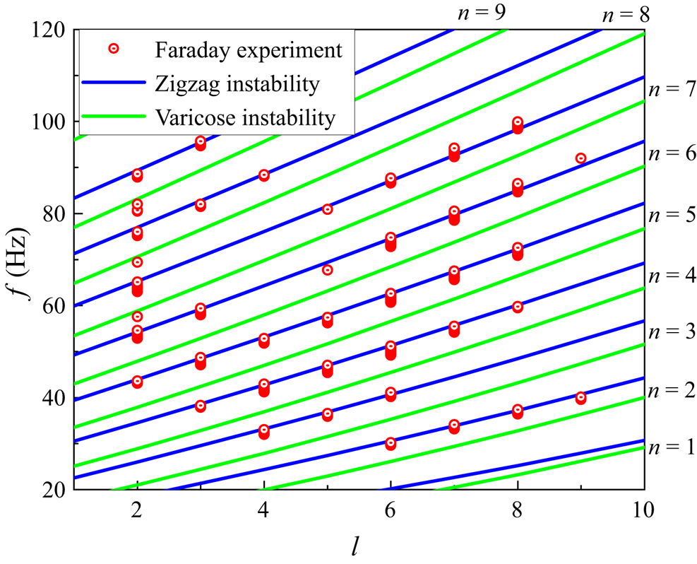
According to the asymptotic analysis, the dispersion relation of Faraday can be described approximately by (4.11), i.e. $\omega \approx \omega _0$. As shown in figure 6, for the zigzag mode, the experimental results and theoretical calculations from (4.11) agree well. Furthermore, the frequency increases as the wavenumbers ($l$ or $n$) increase, which is in line with previous research on Faraday waves (Benjamin & Ursell Reference Benjamin and Ursell1954; Rajchenbach & Clamond Reference Rajchenbach and Clamond2015; Pototsky & Bestehorn Reference Pototsky and Bestehorn2016; Shao et al. Reference Shao, Wilson, Saylor and Bostwick2021c). However, there is a difference between experimental results and predicted data from the dispersion equation (4.11) regarding the varicose mode, which will be explained in detail in § 6.1 when the coupling effects of two interfaces are discussed.

Figure 6.

Comparison of dispersion relations. The red dots are the experimental results of § 5. The blue lines are the calculated results from the dispersion equation of zigzag mode (4.11), while the green lines are from the dispersion equation of the varicose mode (4.11).

In addition, the vibration amplitude required for Faraday waves was acquired, ranging from 30 to 100 Hz with interval 0.2 Hz, as shown in figure 7. The given data points represent the minimum oscillation amplitude required to observe Faraday waves at a specific frequency. Due to the geometric constraints of the experimental vessel, the Faraday waves have discrete wavenumbers, which results in critical amplitudes of oscillation that are distributed over several Faraday tongues (critical stability curves). In figure 7, we plot the fitted three Faraday tongues corresponding to modes $(2,6)$, $(5,2)$, and $(6,7)$, respectively. The extremum points on each Faraday tongue have the minimum critical oscillation amplitude that corresponds to a particular mode. Figure 7 illustrates that as the frequency decreases, the Faraday tongue narrows, and the variation in critical oscillation amplitude becomes more pronounced. Additionally, the distance between Faraday tongues becomes smaller as the frequency increases, because the frequency differences between the modes become smaller. Therefore, a large amount of data is required to find exactly the minimum value of the Faraday tongue that corresponds to a mode.

Figure 7.

Comparison of our experiments with the critical vibration amplitude-driven zigzag mode Faraday wave in Floquet analysis and asymptotic analysis. The dashed lines are the fitted Faraday tongues.

The corresponding critical vibration amplitudes driving the Faraday waves (Faraday threshold), from experiments, Floquet analysis on the Mathieu equations, first-order asymptotic analysis and second-order asymptotic analysis, are displayed in figure 7. One can see that the critical vibration amplitudes obtained by Floquet analysis agree well with the experimental results, particularly in the region with high frequencies.

As can be seen from figure 6, a zigzag mode appears in the experiment. Equation (4.22a) (zigzag mode) is very close to the experimental results, as shown in figure 7.

However, since the asymptotic expression is the first-order asymptotic result of the viscosity, the curve of the asymptotic analysis is slightly lower than that of the Floquet analysis. Furthermore, by adopting (4.17), we calculate the value of the second-order asymptotic and plot it in figure 7. Results suggest that at lower frequencies, the curves generated by the second-order asymptotic are more accurate than those generated by the first-order asymptotic because the second-order asymptotic includes more interfacial coupling effects. However, as shown in figure 7, at low frequencies corresponding to large wavenumbers, there are still discrepancies between theoretical and experimental results. Discrepancies between the results of these approaches decrease with increasing wavenumber (which is directly proportional to frequency). The observed difference between the experimental and theoretical critical vibration amplitudes in the low-frequency region can be attributed to the increase in importance of the viscous coupling effect as the frequency decreases.

6. Faraday instability modes

By analysing the relative displacements of the two interfaces, Pototsky & Bestehorn (Reference Pototsky and Bestehorn2016) identify two types of modes: in-phase and anti-phase. The in-phase displacement corresponds to the zigzag (barotropic) mode, while the anti-phase displacement corresponds to the varicose mode. Nevertheless, the instability criterion of different modes is not well understood. In this section, we investigate further the Faraday instability modes from a theoretical point, and discuss the relationship between the interfacial coupling strength and the instability modes.

Equations (2.19) and (2.20) show that the coupling strength of two interfaces is determined by the dimensionless parameters $\beta _A$ and $\beta _B$, which range from 0 to 1. The region with strong coupling of two interfaces appears when $0 \ll \rho _A,\rho _B<1$, while the region with weak coupling of two interfaces happens when $\rho _A\sim 0$ and $\rho _B\sim 0$, corresponding to the case when (2.19), (2.20) are approximately decoupled.

6.1. Strongly coupled double-interface system

In this subsection, we perform Floquet analysis and find a direct solution of the Mathieu equations (2.19), (2.20) using the parameters at $f=60$ Hz from § 5. The initial conditions of the direct solution are set as $\xi _A = \xi _B = \xi _0$ and $\dot {\xi _A} = \dot {\xi _B} = 0$.

As shown in figure 8(a), the growth rate contours of the solution are calculated using the ODE89 function in MATLAB. The value of growth rate $s$ is obtained by fitting exponentially ($\exp (s_A t)$ and $\exp (s_B t)$) the envelope of the wave amplitude and then selecting the maximum value of the two interface growth rates for presentation. Furthermore, the Faraday tongue (black dotted line in figure 8a) is calculated by Floquet analysis, which is in agreement with the direct solution of the Mathieu equations, except for the narrow third tongue (pink dashed line in figure 8a) near the double-tongue stability curves. Similar to Pototsky & Bestehorn (Reference Pototsky and Bestehorn2016), we also found two instability modes, the zigzag mode (point I), and the varicose mode (point II), as shown in figure 8(a). Two modes correspond to two extremes of double-tongued stability curves of the strongly coupled double-interface system. Figure 8(a) also shows that the zigzag mode is dominant in our experiments because of the lower Faraday threshold. Furthermore, we can use the zero-order approximate equation (4.4) to give an illustration of the occurrence of two instability modes. Substituting (4.7) into (4.4), we obtain

(6.1) \begin{equation} \left.\begin{gathered} \dfrac{\xi_A}{\xi_B} = \dfrac{\omega^2 \beta_A}{\omega^2-\varOmega_A^2},\\ \dfrac{\xi_A}{\xi_B} = \dfrac{\omega^2-\varOmega_B^2}{\omega^2 \beta_B}.\end{gathered}\right\} \end{equation}

Figure 8.

Critical stability curve, growth rate and instability mode of the strongly coupled system and weakly coupled system: (a) strongly coupled double-interface system $h_2=1.262\ \mathrm {mm}$; (b) weakly coupled double-interface system $h_2=12.62\ \mathrm {mm}$; (c) typical modes and instabilities. The growth rate $s$ of waves is calculated by the ODE89 function in the strongly coupled double-interface system, the double-tongued stability curves of Floquet solutions, and the location of the three modes of instability. The black dotted line (the outline of the coloured area) is the first subharmonic stability curve calculated by Floquet analysis. The pink dashed line is the stability curve of the beating mode calculated by the ODE89 function.

The dispersion relation (4.11) can be obtained from (6.1). Furthermore, characteristic frequencies $\omega$ should satisfy $\omega >\max \{ \varOmega _A, \varOmega _B \}$ or $\omega <\min \{ \varOmega _A, \varOmega _B \}$ when $0<(\beta _A, \beta _B)<1$. We notice that when $\omega >\max \{ \varOmega _A, \varOmega _B \}$, $\xi _A/\xi _B>0$, that is, zigzag mode occurs. Similarly, when $\omega <\min \{ \varOmega _A, \varOmega _B \}$, $\xi _A/\xi _B<0$, namely, the varicose mode occurs. It should be noted that these two modes of instability do not alter the characteristics of subharmonic instability. As shown in figure 9(a), the Fourier analysis results show that the wave frequency is concentrated at $\omega$, the subharmonic frequency. Simultaneously, the triple frequency is observed, which can be explained by the first-order asymptotic approximation (4.12), (4.13). Although the results of the Floquet analysis are in good agreement with the direct solution of the Mathieu equations in most cases in figure 8(a), the ordinary differential equation solutions give a narrow third tongue near the double-tongued stability curves in figure 8(a). Figure 9(a) shows that the beating mode that exhibits primary frequencies is found at point III (red solid and dashed lines). Moreover, the average frequency of the beating mode is half of the external excitation frequency. Even though this phenomenon has not yet been found in experiments, we are still able to provide some results from a theoretical analysis. It can be seen from Appendix B that the two primary frequencies of the beating wave are the two characteristic frequencies, $\omega _{0,1}$ and $\omega _{0,2}$, obtained from the dispersion relation. The centre frequency of the beating wave is $(\omega _{0,1}+\omega _{0,2})/2$ in figure 8(a). Figure 9(a) confirms that the frequency difference is $| \omega _{0,1}-\omega _{0,2} |$, and this phenomenon also exists near the triple frequency. The beating mode obtained here is similar to the combination resonances discovered by Kidambi (Reference Kidambi2013). Both are generated by the coupling effects of the system. However, the beating instability involves a dynamic coupling between two interfaces, whereas the coupling involves interactions between different modes induced by a fixed contact line.

Figure 9.

Results of fast Fourier transform in strongly coupled and weakly coupled double-interface systems: (a) strongly coupled double-interface system, $h_2=1.262\ \mathrm {mm}$; (b) weakly coupled double-interface system, $h_2=12.62\ \mathrm {mm}$. The solid line refers to interface $A$, while the dotted line refers to interface $B$, and $\varOmega _w$ is the frequency of the wave.

6.3. Relationship between coupling strength and instability modes

The previous results indicate that changes in coupling strength affect the Faraday instability mode. Under strongly coupled conditions ($0 \ll \beta _A,\beta _B<1$), zigzag mode, varicose mode, and beating mode occur (§ 6.1), while under weakly coupled conditions ($\beta _A,\beta _B \sim 0$), the instabilities of the two interfaces are independent of each other. All instability modes, except the beating mode, satisfy approximately the dispersion relation (4.11). Equation (4.11) gives us two solutions, $\omega _{0,1}$ and $\omega _{0,2}$:

(6.2)\begin{equation} \left.\begin{gathered} \omega_{0,1}=\sqrt{\frac{\varOmega_A^2+\varOmega_B^2+\sqrt{\left(\varOmega_A^2- \varOmega_B^2\right)^2+4 \beta_A \beta_B \varOmega_A^2 \varOmega_B^2}}{2\left(1- \beta_A \beta_B\right)}},\\ \omega_{0,2}=\sqrt{\frac{\varOmega_A^2+\varOmega_B^2-\sqrt{\left(\varOmega_A^2-\varOmega_B^2\right)^2+4 \beta_A \beta_B \varOmega_A^2 \varOmega_B^2}}{2\left(1- \beta_A \beta_B\right)}}. \end{gathered}\right\} \end{equation}

In figure 10(b), data of mode $(3, 4)$ are obtained by substituting (6.2) into any equation in (6.1). As $kh_2$ increases, the zigzag mode transforms gradually into $B$-interface instability, while the varicose mode transitions gradually to $A$-interface instability. This change is caused primarily by the coupling strength of the two interfaces. It can be seen that different instability modes are specific manifestations of the two solutions of the dispersion relation under different coupling degrees. To describe the strength of interface coupling, the parameters $\beta _A$ and $\beta _B$, which come from the derivation of the equation, are used. It can be seen from figure 10(a) that $\beta _A,\beta _B$ decreases rapidly with the increase of $kh_2$. The influences of $\beta _A$ and $\beta _B$ are also reflected in the dispersion relationships, as shown in figure 10(c). As $kh_2$ increases, $\omega _{0,1}$ approaches $\varOmega _A$, and $\omega _{0,1}$ approaches $\varOmega _B$.

Figure 10.

(a) The relationship between coupling strength coefficient $\beta _A, \beta _B$ and dimensionless number $kh_2$ of mode $(3,4)$, where $h_1=12.63\ \textrm {mm}$, $R=27.5\ \textrm {mm}$, $\rho _1 = 6360\ \textrm {kg}\ \textrm {m}^{-3}$ and $\rho _2 = 1041\ \textrm {kg}\ \textrm {m}^{-3}$, calculated by (2.14a,b). (b) The relationship between the amplitude ratio of the two interfaces $\xi _A / \xi _B$ and dimensionless number $kh_2$ of mode $(3, 4)$, calculated by (6.1) and (6.2). (c) The two solid lines are calculated from (6.2), and the two dashed lines are calculated from (2.14a,b), for mode $(3,4)$.

However, in figure 11(b), as $kh_2$ increases for mode $(4, 4)$, zigzag mode transforms gradually to $A$-interface instability, and varicose mode transits to $B$-interface instability. Moreover, figure 11(c) shows that $\omega _{0,1}$ converges to $\varOmega _A$, and $\omega _{0,2}$ converges to $\varOmega _B$ when $\varOmega _A > \varOmega _B$. It is observed in figures 10(c) and 11(c) that the modal conversion directions between mode $(3, 4)$ and mode $(4, 4)$ are related to $\varOmega _A/\varOmega _B$. Assuming $h_j \to \infty$, $k_c=\sqrt {2g( \rho _2^2-\rho _1 \rho _3 )/(\sigma _A( \rho _2+\rho _3 )-\sigma _B( \rho _1+\rho _2 ))}$ is obtained from (2.14a,b) when $\varOmega _A/\varOmega _B=1$, which is the critical wavenumber of the modes transition. From figure 12, when $k< k_c$, $\omega _{0,1}$ converges to $\varOmega _B$, and $\omega _{0,2}$ converges to $\varOmega _A$, similar to the previous discussion of mode $(3,4)$. When $k>k_c$, $\omega _{0,1}$ converges to $\varOmega _A$, and $\omega _{0,2}$ converges to $\varOmega _B$, similar to the previous discussion of mode $(4,4)$.

Figure 11.

(a) The relationship between coupling strength coefficient $\beta _A, \beta _B$ and dimensionless number $kh_2$ of mode $(4,4)$, where $h_1=12.63\ \textrm {mm}$, $R=27.5\ \textrm {mm}$, $\rho _1 = 6360\ \textrm {kg}\ \textrm {m}^{-3}$ and $\rho _2 = 1041\ \textrm {kg}\ \textrm {m}^{-3}$, calculated by (2.14a,b). (b) The relationship between the amplitude ratio of the two interfaces $\xi _A / \xi _B$ and dimensionless number $kh_2$ of mode $(4,4)$, calculated by (6.1) and (6.2). (c) The two solid lines are calculated from (6.2), and the two dashed lines are calculated from (2.14a,b) for mode $(4,4)$.

Figure 12.

The curves of $\varOmega _A/\varOmega _B$, $\omega _{0,1}/\varOmega _A$, $\omega _{0,1}/\varOmega _B$, $\omega _{0,2}/\varOmega _A$ and $\omega _{0,2}/\varOmega _B$ converge at the point $(k_c,1)$, where $R=27.5\ \textrm {mm}$, $\rho _1 = 6360\ \textrm {kg}\ \textrm {m}^{-3}$ and $\rho _2 = 1041\ \textrm {kg}\ \textrm {m}^{-3}$, calculated by (2.14a,b). The wavenumber of mode $(3,4)$ is less than $k_c$, and the wavenumber of mode $(4,4)$ is greater than $k_c$.