2. Geometric variational formulation for MHD

In this section we review the Hamilton principle for ideal MHD as well as the associated Euler–Poincaré variational formulation. We then extend the resulting form of equations to include viscosity and resistivity and examine how the balance of energy, magnetic helicity and cross-helicity emerges from this formulation.

2.1. Lagrangian variational formulation for ideal MHD

Assume that the fluid moves in a compact domain $\varOmega \subset \mathbb {R} ^3$ with a smooth boundary. We denote by $\text {Diff}( \varOmega )$ the group of diffeomorphisms of $\varOmega$ and by $\varphi :[0,T] \rightarrow \text {Diff}( \varOmega )$ the fluid flow. The associated motion of a fluid particle with label $X \in \varOmega$ is $x= \varphi (t,X)$.

When $\nu =0$, the equation for the magnetic field reduces to $\partial _tB - {\rm curl} (u \times B)=0$, which can be equivalently rewritten in geometric terms as $\partial _t (B \cdot \textrm {d}s)+ \unicode{x00A3} _u ( B \cdot \textrm {d} s)=0$ with $\unicode{x00A3} _u(B \cdot \textrm {d}s)$ the Lie derivative of the closed $2$-form $B \cdot \textrm {d}s$. Consequently, from the properties of Lie derivatives, the time evolution of the magnetic field is given by the push-forward operation on 2-forms as

(2.1)\begin{equation} B(t) \cdot \textrm{d}s= \varphi (t)_* ( \mathcal{B}_0 \cdot \textrm{d} S), \end{equation}

for some time-independent reference magnetic field $\mathcal {B} _0(X)$. This describes the fact that the magnetic field is frozen in the flow. Similarly, from the continuity equation $\partial _t \rho + \text {div}( \rho u)=0$, the evolution of the mass density is given by the push-forward operation on 3-forms as

(2.2)\begin{equation} \rho (t)\, \textrm{d}^3 x = \varphi (t)_* ( \varrho _0 \textrm{d}^3X), \end{equation}

for some time-independent reference mass density $\varrho _0(X)$. This discussion, as well as the developments below, are easily adapted to the two-dimensional case $\varOmega \subset \mathbb {R} ^2$ by considering, instead of $B \cdot \textrm {d} s$, the closed $1$-form $B \cdot \textrm {d}\kern0.7pt x$ with $B$ parallel to the plane.

From these considerations, if follows that the ideal MHD motion is completely characterized by the fluid flow $\varphi (t) \in \text {Diff}( \varOmega )$ and the given reference fields $\varrho _0$ and $\mathcal {B} _0$. The Hamilton principle for this system reads

(2.3)\begin{equation} \delta \int_0^T L( \varphi , \partial _t \varphi , \varrho_0, \mathcal{B}_0)\, \textrm{d}t=0, \end{equation}

with respect to variations $\delta \varphi$ vanishing at $t=0,T$, and yields the equations of motion in Lagrangian coordinates. In (2.3), the Lagrangian function $L$ depends on the fluid flow $\varphi (t)$ and its time derivative $\partial _t\varphi (t)$ forming an element $( \varphi , \partial _t \varphi )$ in the tangent bundle $T \text {Diff}( \varOmega )$ to $\text {Diff}( \varOmega )$, and also parametrically on the given $\varrho _0, \mathcal {B} _0$. From the relabelling symmetries, $L$ must be invariant under the subgroup $\text {Diff}( \varOmega )_{ \varrho _0, \mathcal {B}_0 } \subset \text {Diff}( \varOmega )$ of diffeomorphisms that preserve $\varrho _0$ and $\mathcal {B} _0$, i.e. diffeomorphisms $\psi \in \text {Diff}( \varOmega )$ such that

(2.4a,b)\begin{equation} \psi ^*( \varrho _0 \textrm{d}^3X) = \varrho _0\textrm{d}^3X \quad\text{and}\quad \psi ^* ( \mathcal{B} _0 \cdot \textrm{d}S) = \mathcal{B} _0 \cdot \textrm{d}S, \end{equation}

i.e. we have

(2.5)\begin{equation} L( \varphi \circ \psi , \partial _t( \varphi \circ \psi ), \varrho _0, \mathcal{B} _0)= L( \varphi , \partial _t \varphi , \varrho_0, \mathcal{B}_0), \quad \forall\, \psi \in \text{Diff}( \varOmega )_{ \varrho _0, \mathcal{B}_0 } \subset \text{Diff}( \varOmega ) . \end{equation}

From this invariance, $L$ can be written in terms of Eulerian variables as

(2.6)\begin{equation} L( \varphi , \partial _t \varphi , \varrho_0, \mathcal{B}_0)=\ell(u, \rho , B), \end{equation}

(see Remark 2.1) where

(2.7a–c)\begin{equation} u = \partial _t \varphi \circ \varphi ^{{-}1} , \quad \rho \, \textrm{d}^3 x = \varphi _* ( \varrho _0 \textrm{d}^3 X), \quad B \cdot \textrm{ds} = \varphi _* ( \mathcal{B} _0 \cdot \textrm{d} S), \end{equation}

thereby yielding the symmetry reduced Lagrangian $\ell (u, \rho , B)$ in the Eulerian description. In terms of $\ell$, Hamilton's principle (2.3) reads

(2.8)\begin{equation} \delta \int_0^T\ell(u, \rho , B)\, \textrm{d}t=0, \end{equation}

with respect to variations of the form

(2.9a–c)\begin{equation} \delta u = \partial _t v+ \unicode{x00A3} _uv, \quad \delta \rho ={-} \text{div}( \rho v), \quad \delta B = {\rm curl} ( v \times B) , \end{equation}

where $v:[0,T] \rightarrow \mathfrak {X} ( \varOmega )$ is an arbitrary time-dependent vector field with $v(0)=v(T)=0$ and $\unicode{x00A3} _uv=[u,v]$ is the Lie derivative of vector fields. Here, $\mathfrak {X} ( \varOmega )$ denotes the space of vector fields $u$ on $\varOmega$ with $u \cdot n=0$ on $\partial \varOmega$, viewed as the Lie algebra of $\text {Diff}( \varOmega )$. We recall that $B \cdot n=0$ on $\partial \varOmega$, a condition that is preserved by the evolution (2.1). The passing from (2.3) to (2.8) is a special instance of the process of Euler–Poincaré reduction for invariant systems on Lie groups, see Holm, Marsden & Ratiu (Reference Holm, Marsden and Ratiu1998). The expressions for the variations in (2.9a–c) follow by taking the variation of the relations (2.7a–c) with respect to a path $\varphi ^\varepsilon$ of time-dependent diffeomorphisms with fixed endpoints at $t=0,T$. For instance, for the second relation, writing $\rho ^ \varepsilon \, \textrm {d}^3 x = \varphi ^ \varepsilon _* ( \varrho _0 \textrm {d}^3 X)$, one has

(2.10)\begin{align} \delta \rho \, \textrm{d} ^3x &= \left. \frac{\textrm{d}}{\textrm{d} \varepsilon}\right|_{\varepsilon=0}\rho^ \varepsilon \, \textrm{d}^3 x = \left. \frac{\textrm{d}}{\textrm{d} \varepsilon}\right|_{\varepsilon=0} \varphi ^\varepsilon _* ( \varrho _0 \textrm{d}^3 X)={-} \unicode{x00A3} _v ( \varphi _* ( \varrho _0 \textrm{d}^3 X))\nonumber\\ &={-} \unicode{x00A3} _v ( \rho\, \textrm{d} ^3 x)={-} \text{div}( \rho v)\, \textrm{d} ^3 x,\quad\text{with } v= \left. \frac{\textrm{d}}{\textrm{d} \varepsilon}\right|_{\varepsilon=0} \varphi ^ \varepsilon \circ \varphi ^{{-}1}, \end{align}

where we used the definition of the Lie derivative $\unicode{x00A3} _v$. A direct application of (2.8) and (2.9a–c) yields the fluid momentum equations in the form

(2.11)\begin{equation} \left\langle \partial_t \frac{\delta \ell}{\delta u} , v \right\rangle + a\left(\frac{\delta \ell}{\delta u}, u, v\right) + b\left( \frac{\delta \ell}{\delta \rho},\rho,v \right) + c\left(\frac{\delta \ell}{\delta B},B,v\right)=0, \end{equation}

for all $v$ with $v \cdot n=0$, with the trilinear forms

(2.12)\begin{equation} \left.\begin{array}{c@{}} \displaystyle a(w,u,v)={-}\int_ \varOmega w \cdot [u,v]\,\textrm{d}\kern0.7pt x ,\\ \displaystyle b(\sigma , \rho ,v)={-} \int_ \varOmega \rho \boldsymbol{\nabla} \sigma \cdot v \,\textrm{d}\kern0.7pt x,\\ \displaystyle c(C,B,v)= \int_\varOmega C \cdot {\rm curl} (B \times v) \,\textrm{d}\kern0.7pt x. \end{array} \right\} \end{equation}

The equations for $\rho$ and $B$ follow from their definition in (2.7a–c), which are expressed in terms of $b$ and $c$ as

(2.13)\begin{gather} \langle \partial_t \rho, \sigma \rangle + b(\sigma,\rho,u) = 0, \quad \forall\, \sigma, \end{gather}

(2.14)\begin{gather}\langle \partial_t B, C \rangle + c(C,B,u) = 0, \quad \forall\, C, \quad C \cdot n|_{ \partial \varOmega }=0. \end{gather}

Equation (2.11) yields the general Euler–Poincaré form of the equations for arbitrary Lagrangian $\ell (u, \rho , B)$ as

(2.15)\begin{equation} \partial _t \frac{\delta \ell}{\delta u} + \unicode{x00A3} _u \frac{\delta \ell}{\delta u} = \rho \boldsymbol{\nabla} \frac{\delta \ell}{\delta \rho }+ B \times {\rm curl}\frac{\delta \ell}{\delta B} , \end{equation}

where in the second term we employed the notation $\unicode{x00A3} _u m= {\rm curl}\, m\times u + \boldsymbol {\nabla } ( u \cdot m) + m \text {div}u$.

The Lagrangian for barotropic MHD is

(2.16)\begin{equation} \ell(u, \rho , B)= \int_ \varOmega \left[\frac{1}{2} \rho |u|^2 - \epsilon ( \rho ) - \frac{1}{2} |B| ^2 \right]\,\textrm{d}\kern0.7pt x, \end{equation}

with $\epsilon ( \rho )$ the energy density. Using

(2.17a–c)\begin{equation} \frac{\delta \ell}{\delta u}= \rho u, \quad \frac{\delta \ell}{\delta \rho } = \frac{1}{2} |u| ^2 - \frac{\partial \epsilon }{\partial \rho } , \quad \frac{\delta \ell}{\delta B} ={-} B, \end{equation}

in (2.15) yields the barotropic MHD equations (1.1) with $\mu = \lambda =0$.

Extension to full compressible ideal MHD subject to gravitational and Coriolis forces is easily achieved by including the entropy density $s$ in the variational formulation and considering the Lagrangian function

(2.18)\begin{equation} \ell(u, \rho ,s , B)= \int_ \varOmega \left[\frac{1}{2} \rho |u|^2 + \rho R \cdot u - \epsilon ( \rho ,s ) - \rho \phi - \frac{1}{2} |B| ^2\right] \,\textrm{d}\kern0.7pt x, \end{equation}

with $\phi$ the gravitational potential and a vector field $R$ such that ${\rm curl}\,R= 2 \omega$ with $\omega$ the angular velocity of the fluid domain.

Remark 2.1. Lagrangian reduction From the point of view of Lagrangian reduction by symmetry, the passing from $L$ to $\ell$ is justified as follows. Given $\varrho _0$ and $\mathcal {B} _0$, the Lagrangian $L( \cdot , \cdot , \varrho _0, \mathcal {B} _0):T \text {Diff}( \varOmega ) \rightarrow \mathbb {R}$ is $\text {Diff}( \varOmega )_{ \varrho _0, \mathcal {B}_0 }$-invariant, hence it induces a function $\ell : T\text {Diff}( \varOmega ) /\text {Diff}( \varOmega )_{ \varrho _0, \mathcal {B}_0 } \rightarrow \mathbb {R}$, the symmetry reduced Lagrangian, on the quotient of $T \text {Diff}( \varOmega )$ by the symmetry group $\text {Diff}( \varOmega )_{ \varrho _0, \mathcal {B}_0 }$. This quotient space can be identified with the space $\mathfrak {X} ( \varOmega ) \times {O} _{ \varrho _0, \mathcal {B}_0 }$ where ${O} _{ \varrho _0, \mathcal {B}_0 }=\{ \varphi _* ( \varrho _0 \textrm {d}^3 X) , \varphi _*(\mathcal {B} _0 \cdot \textrm {d} S) \mid \varphi \in \text {Diff}( \varOmega )\}$ is the orbit of $(\varrho _0, \mathcal {B}_0)$ under the action of $\text {Diff}( \varOmega )$. The identification is given by

(2.19)\begin{equation} [\varphi , \partial _t \varphi ] \in T\text{Diff}( \varOmega ) /\text{Diff}( \varOmega )_{ \varrho _0, \mathcal{B}_0 } \longmapsto (u, \rho , B)\in \mathfrak{X} ( \varOmega ) \times {O}_{\varrho _0, \mathcal{B}_0}, \end{equation}

where $[ \varphi , \partial _t \varphi ]$ denotes the equivalence class and $(u, \rho , B)$ are defined as in (2.7a–c). Thanks to this identification, the reduced Lagrangian $\ell : \mathfrak {X} ( \varOmega ) \times {O} _{ \varrho _0, \mathcal {B}_0 } \rightarrow \mathbb {R}$ is related to $L$ as written in (2.6). The following diagram illustrates the reduction process.

(2.20)

2.2. Viscous and resistive MHD

Viscosity and resistivity are included in the formulation (2.11)–(2.14) by defining the symmetric bilinear forms

(2.21)\begin{equation} \left.\begin{array}{c@{}} \displaystyle d(u,v)={-} \int_ \varOmega \left[\mu\boldsymbol{\nabla} u: \boldsymbol{\nabla} v + ( \lambda + \mu ) \text{div}\,u \,\text{div}\,v\right]\, \textrm{d}\kern0.7pt x,\\ \displaystyle e(B, C) ={-}\nu \int_\varOmega \,{\rm curl}\,B \cdot {\rm curl}\, C \,\textrm{d}\kern0.7pt x, \end{array}\right\} \end{equation}

and considering the no-slip boundary condition $u|_{ \partial \varOmega }=0$ for the velocity. This corresponds in the Lagrangian description to the choice of the subgroup $\text {Diff}_0( \varOmega )$ of diffeomorphisms fixing the boundary pointwise. The viscous and resistive barotropic MHD equations with Lagrangian $\ell (u, \rho , B)$ can be written as follows: seek $u, \rho , B$ with $u|_{ \partial \varOmega }=0$ and $B \cdot n|_{ \partial \varOmega }=0$ such that

(2.22)\begin{gather} \hspace{-15pc}\left\langle \partial_t \frac{\delta \ell}{\delta u} , v \right\rangle + a\left(\frac{\delta \ell}{\delta u}, u, v\right) \nonumber\\ + b\left( \frac{\delta \ell}{\delta \rho},\rho,v \right) + c\left(\frac{\delta \ell}{\delta B},B,v\right)= d(u,v), \quad \forall\,v, v|_{ \partial \varOmega }=0, \end{gather}

(2.23)\begin{gather} \langle \partial_t \rho, \sigma \rangle + b(\sigma,\rho,u) =0, \quad \forall\,\sigma , \end{gather}

(2.24)\begin{gather}\langle \partial_t B, C \rangle + c(C,B,u) = e(B,C), \quad \forall\, C, C \cdot n|_{ \partial \varOmega}=0. \end{gather}

The boundary condition ${\rm curl}\,B \times n|_{ \partial \varOmega }=0$ emerges from the last equation, while the condition $\text {div}B(t)=0$ holds if it holds at initial time. For the Lagrangian (2.16), the system (1.1)–(1.5) is recovered. While the system (2.22)–(2.24) is obtained by simply appending the bilinear forms $d$ and $e$ to the Euler–Poincaré equations, this system can also be obtained by a variational formulation of Lagrange–d’Alembert type, which extends the Euler–Poincaré formulation (2.8) and (2.9a–c), see Appendix A.

2.3. Balance laws for important quantities

In the Euler–Poincaré formulation (2.22)–(2.24), the balance of total energy $\mathcal {E} = \langle {\delta \ell }/{\delta u},\ u \rangle -\ell (u, \rho , B)$ associated with a given Lagrangian $\ell$ is computed as

(2.25)\begin{align} \frac{\textrm{d}}{\textrm{d} t} \mathcal{E} &= \left\langle \partial _t \frac{\delta \ell}{\delta u}, u \right\rangle - \left\langle \frac{\delta \ell}{\delta \rho }, \partial _t \rho \right\rangle - \left\langle \frac{\delta \ell}{\delta B }, \partial _t B \right\rangle\nonumber\\ & ={-} a\left(\frac{\delta \ell}{\delta u}, u, u\right) - b\left( \frac{\delta \ell}{\delta \rho},\rho, u \right) - c\left(\frac{\delta \ell}{\delta B},B,u\right) + d(u,u)\nonumber\\ & \quad + b\left( \frac{\delta \ell}{\delta \rho},\rho, u \right) + c\left(\frac{\delta \ell}{\delta B},B,u\right) - e \left( B, \frac{\delta \ell}{\delta B} \right)\nonumber\\ & = d(u,u) - e \left( B, \frac{\delta \ell}{\delta B} \right), \end{align}

and follows from the property

(2.26)\begin{equation} a(w,u,v)={-} a(w,v,u), \quad \forall\, u,v,w, \end{equation}

of the trilinear form $a$.

The conservation of total mass $\int _ \varOmega \rho \, \textrm {d}\kern0.7pt x$ follows from the property

(2.27)\begin{equation} b(1, \rho , v)=0, \quad \forall\, \rho , v. \end{equation}

If $A$ is any vector field satisfying ${\rm curl}\,A=B$ and $A \times n|_{ \partial \varOmega }=0$, the balance of magnetic helicity $\int _ \varOmega A \cdot B\textrm {d}\kern0.7pt x$ is found as follows:

(2.28)\begin{align} \frac{\textrm{d}}{\textrm{d} t} \int_ \varOmega A \cdot B\,\textrm{d}\kern0.7pt x&= \langle \partial _t A, B \rangle + \langle A, \partial _t B \rangle \nonumber\\ &= \langle \partial _t A, {\rm curl}\, A \rangle + \langle A, \partial _t B \rangle\nonumber\\ &= \langle {\rm curl}\, \partial _t A, A \rangle + \langle A, \partial _t B \rangle\nonumber\\ &= 2 \langle \partial _t B, A \rangle \nonumber\\ &={-} 2 c(A,B,u)+ 2e(B,A)\nonumber\\ &= 2e(B,A), \end{align}

where in the third equality we used $A \times n|_{ \partial \varOmega }=0$ and the following instance of Stokes’ theorem:

(2.29)\begin{equation} \langle {\rm curl}\,C, D \rangle = \langle C, {\rm curl}\,D \rangle + \int_{ \partial \varOmega } (C \times D) \cdot n \,\textrm{d} s, \end{equation}

for vector fields $C,D$ on $\varOmega$. In the fifth equality we used (2.24) (which holds even if $C \cdot n \neq 0$), and in the last one we used the following property of $c$:

(2.30)\begin{equation} c(A,B,u)=0 \text{ if } B= \text{curl } A \text{ and } u|_{ \partial \varOmega }=0. \end{equation}

In the absence of viscosity, $u|_{ \partial \varOmega }=0$ does not hold and one uses

(2.31)\begin{equation} c(A,B,u)=0 \text{ if } B= {\rm curl}\,A \text{ and } u \cdot n|_{ \partial \varOmega }= B \cdot n|_{ \partial \varOmega }=0. \end{equation}

3. Spatial variational discretization

We will now construct a spatial discretization of (1.1)–(1.6) using finite elements. We make use of the following function spaces:

(3.1)\begin{equation} \left.\begin{array}{c} H^1_0(\varOmega) = \{f \in L^2(\varOmega) \mid \boldsymbol{\nabla} f \in L^2(\varOmega)^d, f=0 \text{ on } \partial\varOmega \}, \\ H_0({\rm curl},\varOmega) = \begin{cases} \{ u \in L^2(\varOmega)^2 \mid \partial_x u_y - \partial_y u_x \in L^2(\varOmega), \, u_x n_y - u_y n_x = 0 \text{ on } \partial\varOmega \}, & \mbox{if } d = 2, \\ \{ u \in L^2(\varOmega)^3 \mid {\rm curl} u \in L^2(\varOmega)^3, \, u \times n = 0 \text{ on } \partial\varOmega \}, & \mbox{if } d = 3, \end{cases} \\ H_0({\rm div},\varOmega) = \{u \in L^2(\varOmega)^d \mid {\rm div} u \in L^2(\varOmega), u \cdot n = 0 \text{ on } \partial\varOmega \}. \end{array}\right\} \end{equation}

Let $\mathcal {T}_h$ be a triangulation of $\varOmega$. We regard $\mathcal {T}_h$ as a member of a family of triangulations parametrized by $h = \max _{K \in \mathcal {T}_h} h_K$, where $h_K = \text {diam}K$ denotes the diameter of a simplex $K$. We assume that this family is shape regular, meaning that the ratio $\max _{K \in \mathcal {T}_h} h_K/\rho _K$ is bounded above by a positive constant for all $h>0$. Here, $\rho _K$ denotes the inradius of $K$.

When $r \ge 0$ is an integer and $K$ is a simplex, we write $P_r(K)$ to denote the space of polynomials on $K$ of degree at most $r$.

Let $r,s \ge 0$ be fixed integers. To discretize the velocity $u$, we use the continuous Galerkin space

(3.2)\begin{equation} U_h^{\textrm{grad}} = CG_{r+1}(\mathcal{T}_h)^d := \{u \in H^1_0(\varOmega)^d \mid u |_K \in P_{r+1}(K)^d, \ \forall \,K \in \mathcal{T}_h\}. \end{equation}

To discretize the magnetic field $B$, we use the Raviart–Thomas space

(3.3)\begin{equation} U_h^{{\rm div}} = RT_r(\mathcal{T}_h) := \{u \in H_0({\rm div},\varOmega) \mid u |_K \in P_r(K)^d + xP_r(K), \ \forall \, K \in \mathcal{T}_h\}. \end{equation}

To discretize the density $\rho$, we use the discontinuous Galerkin space

(3.4)\begin{equation} F_h = DG_s(\mathcal{T}_h) := \{ f \in L^2(\varOmega) \mid f |_K \in P_s(K), \ \forall \, K \in \mathcal{T}_h\}. \end{equation}

Our method will also make use of an auxiliary space, the Nedelec finite element space of the first kind,

(3.5)\begin{align} U_h^{{\rm curl}} &= NED_r(\mathcal{T}_h) \nonumber\\ &:= \begin{cases} \{u \in H_0({\rm curl},\varOmega) \mid u |_K \in P_r(K)^2 + (x_2,-x_1) P_r(K), \, \forall K \in \mathcal{T}_h\}, & \mbox{if } d=2,\\ \{u \in H_0({\rm curl},\varOmega) \mid u |_K \in P_r(K)^3 + x \times P_r(K)^3, \, \forall K \in \mathcal{T}_h\}, & \mbox{if } d=3, \end{cases} \end{align}

which satisfies ${\rm curl} U_h^{{\rm curl}} \subset U_h^{{\rm div}}$.

We will need consistent discretizations of the trilinear forms $a,b,c$ and the bilinear forms $d,e$. To construct these, we introduce some notation (and we caution the reader that we abuse the letters $d$ and $e$ in what follows). Let $\mathcal {E}_h$ denote the set of interior $(d-1)$-dimensional faces in $\mathcal {T}_h$. On a face $e = K_1 \cap K_2 \in \mathcal {E}_h$, we denote the jump and average of a piecewise smooth scalar function $f$ by

(3.6a,b)\begin{equation} [\![ f ]\!] = f_1 n_1 + f_2 n_2, \quad \{ f \} = \frac{f_1+f_2}{2}, \end{equation}

where $f_i = f |_{K_i}, n_1$ is the normal vector to $e$ pointing from $K_1$ to $K_2$, and similarly for $n_2$. From now on we focus on dimension $d=3$, as the two-dimensional case follows from trivial modifications, see §4.1.1. We let ${\rm \pi} _h^{\textrm {grad}} : L^2(\varOmega )^3 \rightarrow U_h^{\textrm {grad}}, {\rm \pi}_h^{{\rm curl}} : L^2(\varOmega )^3 \rightarrow U_h^{{\rm curl}}, {\rm \pi}_h^{{\rm div}} : L^2(\varOmega )^3 \rightarrow U_h^{{\rm div}}$ and ${\rm \pi} _h : L^2(\varOmega ) \rightarrow F_h$ denote the $L^2$-orthogonal projectors onto $U_h^{\textrm {grad}}, U_h^{{\rm curl}}, U_h^{{\rm div}}$ and $F_h$, respectively. We define ${\rm curl}_h : U_h^{{\rm div}} \rightarrow U_h^{{\rm curl}}$ by

(3.7)\begin{equation} \langle {\rm curl}_h u, v \rangle = \langle u, {\rm curl} v \rangle, \quad \forall \,v \in U_h^{{\rm curl}}. \end{equation}

We define trilinear forms $b_h : F_h \times F_h \times U_h^{{\rm div}} \rightarrow \mathbb {R}, c_h : L^2(\varOmega )^3 \times U_h^{{\rm div}} \times U_h^{\textrm {grad}} \rightarrow \mathbb {R}$ and a bilinear form $e_h : U_h^{{\rm div}} \times U_h^{{\rm div}} \rightarrow \mathbb {R}$ by

(3.8)\begin{equation} \left.\begin{array}{c@{}} \displaystyle b_h(f,g,u) ={-}\sum_{K \in \mathcal{T}_h} \int_K (u \boldsymbol{\cdot} \boldsymbol{\nabla} f) g \, \textrm{d}\kern0.7pt x + \sum_{e \in \mathcal{E}_h} \int_e u \cdot [\![ f ]\!] \{g\} \, \textrm{d}s, \\ c_h(C,B,v) = \langle C, {\rm curl} {\rm \pi}_h^{{\rm curl}} ({\rm \pi}_h^{{\rm curl}}B \times {\rm \pi}_h^{{\rm curl}}v) \rangle, \\ e_h(B,C)={-}\nu \langle {\rm curl}_h B, {\rm curl}_h C \rangle. \end{array}\right\} \end{equation}

Note that $b_h$ trivially satisfies the property (2.27), ensuring mass conservation. Our choice of $c_h$ is motivated in part by the following lemma which shows that $c_h$ satisfies the property (2.30) of $c$.

Lemma 3.1 The trilinear form $c_h$ satisfies

(3.9)\begin{equation} c_h(w,u,v) = 0\quad \text{if } {\rm curl} w = u. \end{equation}

Proof. If ${\rm curl} w = u$, then we can integrate $c_h$ by parts and use the fact that $n \times {\rm \pi}_h^{{\rm curl}} ({\rm \pi} _h^{{\rm curl}}u \times {\rm \pi}_h^{{\rm curl}}v)|_{\partial \varOmega } = 0$ to obtain

(3.10)\begin{align} c_h(w,u,v)&= \langle w, {\rm curl} {\rm \pi}_h^{{\rm curl}} ({\rm \pi}_h^{{\rm curl}}u \times {\rm \pi}_h^{{\rm curl}}v) \rangle \nonumber\\ &= \langle {\rm curl} w, {\rm \pi}_h^{{\rm curl}} ({\rm \pi}_h^{{\rm curl}}u \times {\rm \pi}_h^{{\rm curl}}v) \rangle \nonumber\\ &= \langle u, {\rm \pi}_h^{{\rm curl}} ({\rm \pi}_h^{{\rm curl}}u \times {\rm \pi}_h^{{\rm curl}}v) \rangle \nonumber\\ &= \langle {\rm \pi}_h^{{\rm curl}} u, {\rm \pi}_h^{{\rm curl}}u \times {\rm \pi}_h^{{\rm curl}}v \rangle \nonumber\\ &= 0. \end{align}

In the spatially discrete, temporally continuous setting, our method seeks $u : [0,T] \rightarrow U_h^{\textrm {grad}}, \rho : [0,T] \rightarrow F_h$ and $B : [0,T] \rightarrow U_h^{{\rm div}}$ such that

(3.11)\begin{gather} \langle \sigma, \partial_t \rho \rangle ={-}b_h(\sigma,\rho,u), \quad \forall\, \sigma \in F_h, \end{gather}

(3.12)\begin{gather}\langle C, \partial_t B \rangle ={-}c_h(C,B,u), \quad \forall \, C \in U_h^{{\rm div}}, \end{gather}

and

(3.13)\begin{equation} \delta \int_0^T \ell(u,\rho,B) \, \textrm{d}t = 0, \end{equation}

for all variations $\delta u : [0,T] \rightarrow U_h^{\textrm {grad}}, \delta \rho : [0,T] \rightarrow F_h$, and $\delta B : [0,T] \rightarrow U_h^{{\rm div}}$ satisfying

(3.14)\begin{gather} \langle w, \delta u \rangle = \langle w, \partial_t v \rangle - a(w,u,v), \quad \forall \, w \in U_h^{\textrm{grad}}, \end{gather}

(3.15)\begin{gather}\langle \sigma, \delta \rho \rangle ={-}b_h(\sigma,\rho,v), \quad \forall\,\sigma \in F_h, \end{gather}

(3.16)\begin{gather}\langle C, \delta B \rangle ={-}c_h(C,B,v), \quad \forall \, C \in U_h^{{\rm div}}, \end{gather}

where $v : [0,T] \rightarrow U_h^{\textrm {grad}}$ is an arbitrary vector field satisfying $v(0)=v(T)=0$.

Note that (3.11) and (3.12) and (3.14)–(3.16) are discrete counterparts of the advection laws

(3.17a,b)\begin{equation} \partial_t \rho ={-}{\rm div}(\rho u), \quad \partial_t B = {\rm curl} (u \times B), \end{equation}

and the constraints

(3.18a–c)\begin{equation} \delta u = \partial_t v + [u,v], \quad \delta \rho ={-}{\rm div}(\rho v), \quad \delta B = {\rm curl}(v \times B), \end{equation}

on the variations.

As shown in Gawlik & Gay-Balmaz (Reference Gawlik and Gay-Balmaz2020b), in the absence of $B$ this variational principle follows from the Hamilton principle on a discrete diffeomorphism group $G_h \subset GL(F_h)$ by applying Euler–Poincaré reduction. In particular, the discrete version of $a$ emerging from the Euler–Poincaré variational formulation in Gawlik & Gay-Balmaz (Reference Gawlik and Gay-Balmaz2020b) coincides with $a$ on the finite element space $U_h^{\textrm {grad}}$ used here for the velocity.

The variational principle above yields the following equations for $u \in U_h^{\textrm {grad}}, \rho \in F_h, B \in U_h^{{\rm div}}$:

(3.19)\begin{gather} \hspace{-13pc}\left\langle \partial_t \frac{\delta \ell}{\delta u}, v \right\rangle + a\left({\rm \pi}_h^{\textrm{grad}} \frac{\delta \ell}{\delta u}, u, v\right)\nonumber\\ + b_h\left( {\rm \pi}_h \frac{\delta \ell}{\delta \rho},\rho,v \right)+ c_h\left({\rm \pi}_h^{{\rm div}} \frac{\delta \ell}{\delta B},B,v\right)= 0, \quad \forall \, v \in U_h^{\textrm{grad}}, \end{gather}

(3.20)\begin{gather} \langle \partial_t \rho, \sigma \rangle + b_h(\sigma,\rho,u) =0, \quad \forall \, \sigma \in F_h, \end{gather}

(3.21)\begin{gather}\langle \partial_t B, C \rangle + c_h(C,B,u) = 0, \quad \forall \, C \in U_h^{{\rm div}}. \end{gather}

We introduce viscosity and resistivity by adding $d(u,v)$ and $e_h(B,C)$ to the right-hand sides of (3.19) and (3.21). The resulting equations read

(3.22)\begin{gather} \hspace{-17pc}\left\langle \partial_t \frac{\delta \ell}{\delta u}, v \right\rangle + a\left({\rm \pi}_h^{\textrm{grad}} \frac{\delta \ell}{\delta u}, u, v\right)\nonumber\\ + b_h\left( {\rm \pi}_h \frac{\delta \ell}{\delta \rho},\rho,v \right) + c_h\left({\rm \pi}_h^{{\rm div}} \frac{\delta \ell}{\delta B},B,v\right)= d(u,v), \quad \forall \, v \in U_h^{\textrm{grad}} , \end{gather}

(3.23)\begin{gather} \langle \partial_t \rho, \sigma \rangle + b_h(\sigma,\rho,u) =0, \quad \forall \, \sigma \in F_h, \end{gather}

(3.24)\begin{gather}\langle \partial_t B, C \rangle + c_h(C,B,u) = e_h(B,C),\quad \forall \, C \in U_h^{{\rm div}}. \end{gather}

These equations are not implementable in their present form, since the terms involving $c_h$ and $e_h$ contain projections of the test functions $v$ and $C$. To handle these terms, we use the following lemma.

Lemma 3.2 Let $u,B \in U_h^{{\rm div}}$ be arbitrary, and let $J,H,U,E,\alpha ,j \in U_h^{{\rm curl}}$ be defined by the relations

(3.25)\begin{gather} \langle J, K \rangle ={-}\left\langle \frac{\delta \ell}{\delta B}, {\rm curl} K \right\rangle, \quad \forall \, K \in U_h^{{\rm curl}}, \end{gather}

(3.26)\begin{gather}\langle H, G \rangle = \langle B, G \rangle, \quad \forall \, G \in U_h^{{\rm curl}}, \end{gather}

(3.27)\begin{gather}\langle U, V \rangle = \langle u, V \rangle, \quad \forall \, V \in U_h^{{\rm curl}}, \end{gather}

(3.28)\begin{gather}\langle E, F \rangle ={-}\langle U \times H, F \rangle, \quad \forall \, F \in U_h^{{\rm curl}}, \end{gather}

(3.29)\begin{gather}\langle \alpha, \beta \rangle ={-}\langle J \times H, \beta \rangle, \quad \forall \, \beta \in U_h^{{\rm curl}}, \end{gather}

(3.30)\begin{gather}\langle j, k \rangle = \langle B, {\rm curl} k \rangle, \quad \forall \, k \in U_h^{{\rm curl}}. \end{gather}

Then, for every $C \in U_h^{{\rm div}}$ and every $v \in U_h^{\textrm{grad}}$, we have

(3.31)\begin{gather} c_h(C,B,u) = \langle {\rm curl} E, C \rangle, \end{gather}

(3.32)\begin{gather}c_h\left({\rm \pi}_h^{{\rm div}}\frac{\delta \ell}{\delta B},B,v\right) = \langle \alpha, v \rangle, \end{gather}

(3.33)\begin{gather}e_h(B,C) ={-}\nu\langle {\rm curl} j, C \rangle. \end{gather}

Proof. We have $H={\rm \pi} _h^{{\rm curl}} B$ and $U = {\rm \pi}_h^{{\rm curl}} u$ by definition. Thus, (3.28) implies that

(3.34)\begin{equation} E ={-}{\rm \pi}_h^{{\rm curl}}(U \times H) ={-}{\rm \pi}_h^{{\rm curl}} ({\rm \pi}_h^{{\rm curl}} u \times {\rm \pi}_h^{{\rm curl}} B). \end{equation}

It follows that

(3.35)\begin{equation} \langle {\rm curl} E, C \rangle ={-}\langle {\rm curl} {\rm \pi}_h^{{\rm curl}} ({\rm \pi}_h^{{\rm curl}} u \times {\rm \pi}_h^{{\rm curl}} B), C \rangle = c_h(C,B,u). \end{equation}

To prove (3.32), we use the fact that ${\rm curl} U_h^{{\rm curl}} \subset U_h^{{\rm div}}$ to write

(3.36)\begin{align} \langle \alpha, v \rangle&= \langle \alpha, {\rm \pi}_h^{{\rm curl}} v \rangle \nonumber\\ &={-}\langle J \times {\rm \pi}_h^{{\rm curl}} B, {\rm \pi}_h^{{\rm curl}} v \rangle \nonumber\\ &={-}\langle J, {\rm \pi}_h^{{\rm curl}} B \times {\rm \pi}_h^{{\rm curl}} v \rangle \nonumber\\ &={-}\langle J, {\rm \pi}_h^{{\rm curl}} ({\rm \pi}_h^{{\rm curl}} B \times {\rm \pi}_h^{{\rm curl}} v) \rangle \nonumber\\ &= \left\langle \frac{\delta\ell}{\delta B}, {\rm curl} {\rm \pi}_h^{{\rm curl}} ({\rm \pi}_h^{{\rm curl}}B \times {\rm \pi}_h^{{\rm curl}}v) \right\rangle \nonumber\\ &= \left\langle {\rm \pi}_h^{{\rm div}} \frac{\delta\ell}{\delta B}, {\rm curl} {\rm \pi}_h^{{\rm curl}} ({\rm \pi}_h^{{\rm curl}}B \times {\rm \pi}_h^{{\rm curl}}v) \right\rangle \nonumber\\ &= c_h\left( {\rm \pi}_h^{{\rm div}} \frac{\delta\ell}{\delta B},B,v\right). \end{align}

Finally, (3.33) follows from the fact that $j = {\rm curl}_h B$ by definition, so

(3.37)\begin{equation} -\nu\langle {\rm curl} j, C \rangle ={-}\nu \langle j, {\rm curl}_h C \rangle = e_h(B,C). \end{equation}

The preceding lemma shows that (3.22)–(3.24) can be rewritten in the following equivalent way. We seek $u,w \in U_h^{\textrm {grad}}, B \in U_h^{{\rm div}}, \rho ,\theta \in F_h$, and $J,H,U,E,\alpha ,j \in U_h^{{\rm curl}}$ such that

(3.38)\begin{gather} \left\langle \partial_t \frac{\delta \ell}{\delta u}, v \right\rangle + a(w, u, v) + b_h(\theta,\rho,v) + \langle \alpha, v \rangle = d(u,v), \quad \forall \, v \in U_h^{\textrm{grad}}, \end{gather}

(3.39)\begin{gather}\langle \partial_t \rho, \sigma \rangle + b_h(\sigma,\rho,u) = 0, \quad \forall \, \sigma \in F_h, \end{gather}

(3.40)\begin{gather}\langle \partial_t B, C \rangle + \langle {\rm curl} E, C \rangle ={-}\nu \langle {\rm curl} j, C \rangle, \quad \forall \, C \in U_h^{{\rm div}}, \end{gather}

(3.41)\begin{gather}\langle w, z \rangle = \left\langle \frac{\delta \ell}{\delta u}, z \right\rangle, \quad \forall \, z \in U_h^{\textrm{grad}}, \end{gather}

(3.42)\begin{gather}\langle \theta, \tau \rangle = \left\langle \frac{\delta \ell}{\delta \rho}, \tau \right\rangle, \quad \forall \, \tau \in F_h, \end{gather}

(3.43)\begin{gather}\langle J, K \rangle ={-}\left\langle \frac{\delta \ell}{\delta B}, {\rm curl} K \right\rangle, \quad \forall \, K \in U_h^{{\rm curl}}, \end{gather}

(3.44)\begin{gather}\langle H, G \rangle = \langle B, G \rangle, \quad \forall \, G \in U_h^{{\rm curl}}, \end{gather}

(3.45)\begin{gather}\langle U, V \rangle = \langle u, V \rangle, \quad \forall \, V \in U_h^{{\rm curl}}, \end{gather}

(3.46)\begin{gather}\langle E, F \rangle ={-}\langle U \times H, F \rangle, \quad \forall \, F \in U_h^{{\rm curl}}, \end{gather}

(3.47)\begin{gather}\langle \alpha, \beta \rangle ={-}\langle J \times H, \beta \rangle, \quad \forall \, \beta \in U_h^{{\rm curl}}, \end{gather}

(3.48)\begin{gather}\langle j, k \rangle = \langle B, {\rm curl} k \rangle, \quad \forall \, k \in U_h^{{\rm curl}}. \end{gather}

Proposition 3.3 If $B(0)$ is exactly divergence free, then the solution to (3.38)–(3.48) satisfies

(3.49)\begin{gather} {\rm div} B(t) \equiv 0, \end{gather}

(3.50)\begin{gather}\frac{\textrm{d}}{\textrm{d} t} \int_\varOmega \rho \, \textrm{d}\kern0.7pt x = 0, \end{gather}

(3.51)\begin{gather}\frac{\textrm{d}}{\textrm{d} t} \mathcal{E} = d(u,u) - e_h\left(B, {\rm \pi}_h^{{\rm div}} \frac{\delta \ell}{\delta B} \right), \end{gather}

(3.52)\begin{gather}\frac{\textrm{d}}{\textrm{d} t} \int_\varOmega A \cdot B \, \textrm{d}\kern0.7pt x = 2e_h(B,{\rm \pi}_h^{{\rm div}} A), \end{gather}

for all $t$. Here, $\mathcal {E} = \langle {\delta \ell }/{\delta u},\ u \rangle - \ell (u,\rho ,B)$ denotes the total energy of the system, and $A$ denotes any vector field satisfying ${\rm curl}\, A = B$ and $A \times n |_{\partial \varOmega } = 0$.

Proof. Since ${\rm curl} U_h^{{\rm curl}} \subset U_h^{{\rm div}}$, the magnetic field equation (3.40) implies that the relation

(3.53)\begin{equation} \partial_t B + {\rm curl} E ={-}\nu {\rm curl} j, \end{equation}

holds pointwise. Taking the divergence of both sides shows that $\partial _t {\rm div} B = 0$, so $B(t)$ is divergence free for all $t$.

Taking $\sigma =1$ in the density (3.39) shows that

(3.54)\begin{equation} \frac{\textrm{d}}{\textrm{d} t} \int_\varOmega \rho \, \textrm{d}\kern0.7pt x = \langle \partial_t \rho, 1 \rangle ={-}b_h(1,\rho,u) = 0. \end{equation}

To compute the rate of change of the energy, we take $v=u$ in (3.22), $\sigma =-{\rm \pi} _h ({\delta \ell }/{\delta \rho })$ in (3.23), and $C=-{\rm \pi} _h^{{\rm div}} ({\delta \ell }/{\delta B})$ in (3.24). Adding the three equations yields

(3.55)\begin{equation} \left\langle \partial_t \frac{\delta \ell}{\delta u}, u \right\rangle - \langle \partial_t \rho, {\rm \pi}_h \frac{\delta\ell}{\delta \rho} \rangle - \left\langle \partial_t B, {\rm \pi}_h^{{\rm div}} \frac{\delta \ell}{\delta B} \right\rangle = d(u,u) - e_h\left(B, {\rm \pi}_h^{{\rm div}} \frac{\delta \ell}{\delta B} \right). \end{equation}

Since $\partial _t \rho \in F_h$ and $\partial _t B \in U_h^{{\rm div}}$, this simplifies to

(3.56)\begin{equation} \left\langle \partial_t \frac{\delta \ell}{\delta u}, u \right\rangle - \left\langle \partial_t \rho, \frac{\delta\ell}{\delta \rho} \right\rangle - \left\langle \partial_t B, \frac{\delta \ell}{\delta B} \right\rangle = d(u,u) - e_h\left(B, {\rm \pi}_h^{{\rm div}} \frac{\delta \ell}{\delta B} \right), \end{equation}

which is equivalent to

(3.57)\begin{equation} \frac{\textrm{d}}{\textrm{d} t} \left( \left\langle \frac{\delta \ell}{\delta u}, u \right\rangle - \ell(u,\rho,B) \right) = d(u,u) - e_h\left(B, {\rm \pi}_h^{{\rm div}} \frac{\delta \ell}{\delta B} \right). \end{equation}

For the magnetic helicity, we compute

(3.58)\begin{align} \frac{\textrm{d}}{\textrm{d} t} \int_ \varOmega A \cdot B \, \textrm{d}\kern0.7pt x &= \langle \partial _t A, B \rangle + \langle A, \partial _t B \rangle \nonumber\\ &= \langle \partial _t A, {\rm curl} A \rangle + \langle A, \partial _t B \rangle\nonumber\\ &= \langle {\rm curl} \partial _t A, A \rangle + \langle A, \partial _t B \rangle\nonumber\\ &= 2 \langle \partial _t B, A \rangle \nonumber\\ &= 2 \langle \partial _t B, {\rm \pi}_h^{{\rm div}} A \rangle \nonumber\\ &={-} 2 c_h({\rm \pi}_h^{{\rm div}} A,B,u)+ 2e_h(B,{\rm \pi}_h^{{\rm div}} A). \end{align}

Since ${\rm curl} U_h^{{\rm curl}} \subset U_h^{{\rm div}}$, we have

(3.59)\begin{align} c_h({\rm \pi}_h^{{\rm div}} A,B,u) &= \langle {\rm \pi}_h^{{\rm div}} A, {\rm curl} {\rm \pi}_h^{{\rm curl}}({\rm \pi}_h^{{\rm curl}}B \times {\rm \pi}_h^{{\rm curl}} u) \rangle \nonumber\\ &= \langle A, {\rm curl} {\rm \pi}_h^{{\rm curl}}({\rm \pi}_h^{{\rm curl}}B \times {\rm \pi}_h^{{\rm curl}} u) \rangle \nonumber\\ &= c_h(A,B,u). \end{align}

Thus,

(3.60)\begin{equation} \frac{\textrm{d}}{\textrm{d} t} \int_ \varOmega A \cdot B \, \textrm{d}\kern0.7pt x ={-} 2 c_h(A,B,u)+ 2e_h(B, {\rm \pi}_h^{{\rm div}} A). \end{equation}

The first term vanishes by Lemma 3.1, yielding (3.52).

Remark 3.4 The proposition above continues to hold if we omit the projection of ${\delta \ell }/{\delta u}$ onto $U_h^{\textrm {grad}}$ in (3.41). We find it advantageous to omit this projection for efficiency. As an illustration, let us consider the setting where $\ell (u,\rho ,B) = \int _\varOmega [\frac {1}{2}\rho |u|^2 - \epsilon (\rho ) - \frac {1}{2}|B|^2] \, \textrm {d}\kern0.7pt x$. If we omit (3.41) and invoke Remark 3.1, then the method seeks $u \in U_h^{\textrm {grad}}, B \in U_h^{{\rm div}}, \rho ,\theta \in F_h$ and $J,H,U,E,\alpha \in U_h^{{\rm curl}}$ such that

(3.61)\begin{gather} \langle \partial_t (\rho u), v \rangle + a(\rho u, u, v) + b_h(\theta,\rho,v) + \langle \alpha, v \rangle = d(u,v), \quad \forall \, v \in U_h^{\textrm{grad}}, \end{gather}

(3.62)\begin{gather}\langle \partial_t \rho, \sigma \rangle + b_h(\sigma,\rho,u) = 0, \quad \forall \, \sigma \in F_h, \end{gather}

(3.63)\begin{gather}\langle \partial_t B, C \rangle + \langle {\rm curl} E, C \rangle ={-}\nu \langle {\rm curl} J, C \rangle, \quad \forall \, C \in U_h^{{\rm div}}, \end{gather}

(3.64)\begin{gather}\langle \theta, \tau \rangle = \left\langle \frac{1}{2}|u|^2 - \frac{\partial \epsilon}{\partial \rho}, \tau \right\rangle, \quad \forall \, \tau \in F_h, \end{gather}

(3.65)\begin{gather}\langle J, K \rangle = \langle B, {\rm curl} K \rangle, \quad \forall \, K \in U_h^{{\rm curl}}, \end{gather}

(3.66)\begin{gather}\langle H, G \rangle = \langle B, G \rangle, \quad \forall \, G \in U_h^{{\rm curl}}, \end{gather}

(3.67)\begin{gather}\langle U, V \rangle = \langle u, V \rangle, \quad \forall \, V \in U_h^{{\rm curl}}, \end{gather}

(3.68)\begin{gather}\langle E, F \rangle ={-}\langle U \times H, F \rangle, \quad \forall \, F \in U_h^{{\rm curl}}, \end{gather}

(3.69)\begin{gather}\langle \alpha, \beta \rangle ={-}\langle J \times H, \beta \rangle, \quad \forall \, \beta \in U_h^{{\rm curl}}. \end{gather}

In this setting, the energy identity (3.51) becomes

(3.70)\begin{equation} \frac{\textrm{d}}{\textrm{d} t} \int_\varOmega \left[\frac{1}{2} \rho |u|^2 + \epsilon(\rho) + \frac{1}{2} |B|^2 \right]\, \textrm{d}\kern0.7pt x = d(u,u) + e_h(B,B). \end{equation}

4. Temporal discretization

In this section, we design a temporal discretization of (3.61)–(3.69) for Lagrangians of the form

(4.1)\begin{equation} \ell(u,\rho,B) = \int_\varOmega \left[\frac{1}{2}\rho|u|^2 - \epsilon(\rho) - \frac{1}{2}|B|^2\right] \, \textrm{d}\kern0.7pt x. \end{equation}

Our temporal discretization will retain all of the structure-preserving properties of our spatial discretization: energy balance, magnetic helicity balance, total mass conservation and ${\rm div} B = 0$.

We adopt the following notation. For a fixed time step $\Delta t > 0$, we denote $t_k = k\Delta t$. The value of the approximate solution $u \in U_h^{\textrm {grad}}$ at time $t_k$ is denoted $u_k$, and likewise for $\rho$ and $B$. The auxiliary variables $\theta \in F_h$ and $J,H,U,E,\alpha \in U_h^{{\rm curl}}$ will play a role in our calculations, but, to reduce notational clutter, we do not index them with a subscript $k$. We write $u_{k+1/2} = ({u_k+u_{k+1}})/{2}, \rho _{k+1/2} = ({\rho _k+\rho _{k+1}})/{2}, B_{k+1/2} = ({B_k+B_{k+1}})/{2}$ and $(\rho u)_{k+1/2} = ({\rho _k u_k+\rho _{k+1} u_{k+1}})/{2}$.

Given $u_k, \rho _k, B_k$, our method steps from time $t_k$ to $t_{k+1}$ by solving

(4.2)\begin{gather} \hspace{-6pc}\left\langle \frac{\rho_{k+1} u_{k+1} - \rho_k u_k}{\Delta t}, v \right\rangle + a\left((\rho u)_{k+1/2}, u_{k+1/2}, v\right) \nonumber\\ + b_h(\theta,\rho_{k+1/2},v) + \langle \alpha, v \rangle = d(u_{k+1/2},v), \quad \forall \, v \in U_h^{\textrm{grad}}, \end{gather}

(4.3)\begin{gather} \left\langle \frac{\rho_{k+1}-\rho_k}{\Delta t}, \sigma \right\rangle + b_h(\sigma,\rho_{k+1/2},u_{k+1/2}) = 0, \quad \forall \, \sigma \in F_h, \end{gather}

(4.4)\begin{gather}\left\langle \frac{B_{k+1}-B_k}{\Delta t}, C \right\rangle + \langle {\rm curl} E, C \rangle ={-}\nu \langle {\rm curl} J, C \rangle, \quad \forall \, C \in U_h^{{\rm div}}, \end{gather}

for $u_{k+1},\rho _{k+1},B_{k+1}$. Here, $\theta , \alpha , E$ and $J$ (as well as $H$ and $U$) are defined by

(4.5)\begin{gather} \langle \theta, \tau \rangle = \langle \tfrac{1}{2}u_k \cdot u_{k+1} - \delta(\rho_k,\rho_{k+1}), \tau \rangle, \quad \forall \, \tau \in F_h, \end{gather}

(4.6)\begin{gather}\langle J, K \rangle = \langle B_{k+1/2}, {\rm curl} K \rangle, \quad \forall \, K \in U_h^{{\rm curl}}, \end{gather}

(4.7)\begin{gather}\langle H, G \rangle = \langle B_{k+1/2}, G \rangle, \quad \forall \, G \in U_h^{{\rm curl}}, \end{gather}

(4.8)\begin{gather}\langle U, V \rangle = \langle u_{k+1/2}, V \rangle, \quad \forall \, V \in U_h^{{\rm curl}}, \end{gather}

(4.9)\begin{gather}\langle E, F \rangle ={-}\langle U \times H, F \rangle, \quad \forall \, F \in U_h^{{\rm curl}}, \end{gather}

(4.10)\begin{gather}\langle \alpha, \beta \rangle ={-}\langle J \times H, \beta \rangle, \quad \forall \, \beta \in U_h^{{\rm curl}}. \end{gather}

In (4.5) we introduced the bivariate function

(4.11)\begin{equation} \delta(x,y) = \frac{\epsilon(y)-\epsilon(x)}{y-x}, \end{equation}

see formula (4.14) below for the justification.

Notice that we used the midpoint rule everywhere above except in the definition of $\theta$, where we used

(4.12)\begin{equation} \tfrac{1}{2}u_k \cdot u_{k+1} - \delta(\rho_k,\rho_{k+1}), \end{equation}

instead of

(4.13)\begin{equation} \frac{1}{2} |u_{k+1/2}|^2 - \left.\frac{\partial\epsilon}{\partial\rho}\right|_{\rho=\rho_{k+1/2}}, \end{equation}

to discretize $\frac {1}{2} |u|^2 -{\partial \epsilon }/{\partial \rho }$. This will allow us to take advantage of the identity

(4.14)\begin{align} &\frac{1}{\Delta t} \int_\varOmega \left[ \frac{1}{2}\rho_{k+1} |u_{k+1}|^2 + \epsilon(\rho_{k+1}) - \frac{1}{2} \rho_k |u_k|^2 - \epsilon(\rho_k)\right] \, \textrm{d}\kern0.7pt x \nonumber\\ &\quad = \left\langle \frac{\rho_{k+1} u_{k+1} - \rho_k u_k}{ \Delta t }, \frac{u_k+u_{k+1}}{2} \right\rangle - \left\langle \frac{\rho_{k+1}-\rho_k}{\Delta t}, \frac{1}{2} u_k \cdot u_{k+1} - \delta(\rho_k,\rho_{k+1}) \right\rangle, \end{align}

when we prove energy conservation below.

Proposition 4.1 If $B_0$ is exactly divergence free, then the solution to (4.2)–(4.10) satisfies

(4.15)\begin{gather} {\rm div} B_k \equiv 0, \end{gather}

(4.16)\begin{gather}\int_\varOmega \rho_{k+1} \, \textrm{d}\kern0.7pt x = \int_\varOmega \rho_k \, \textrm{d}\kern0.7pt x, \end{gather}

(4.17)\begin{gather}\frac{\mathcal{E}_{k+1}-\mathcal{E}_k}{\Delta t} = d(u_{k+1/2},u_{k+1/2}) + e_h(B_{k+1/2}, B_{k+1/2}), \end{gather}

(4.18)\begin{gather}\frac{1}{\Delta t} \left[\int_\varOmega A_{k+1} \cdot B_{k+1} \, \textrm{d}\kern0.7pt x - \int_\varOmega A_k \cdot B_k \, \textrm{d}\kern0.7pt x \right] = 2e_h(B_{k+1/2},{\rm \pi}_h^{{\rm div}} A_{k+1/2}), \end{gather}

for all $k$. Here, $\mathcal {E}_k = \langle {\delta \ell }/{\delta u_k}, u_k \rangle - \ell (u_k,\rho _k,B_k)$ denotes the total energy of the system, and $A_k$ denotes any vector field satisfying ${\rm curl}\, A_k = B_k$ and $A_k \times n |_{\partial \varOmega } = 0$.

Proof. The magnetic field equation (4.4) implies that the relation

(4.19)\begin{equation} \frac{B_{k+1}-B_k}{\Delta t} + {\rm curl} E ={-}\nu {\rm curl} J, \end{equation}

holds pointwise, so taking the divergence of both sides proves (4.15). Conservation of total mass (i.e. (4.16)) is proved by taking $\sigma \equiv 1$ in the density (4.3).

To prove (4.17) and (4.18), we introduce some notation. Let $D_{\Delta t} (\rho u) = (\rho _{k+1} u_{k+1} - \rho _k u_k)/{\Delta t}, D_{\Delta t} B = ({B_{k+1}-B_k})/{\Delta t}$, etc. To reduce notational clutter, we will suppress the subscript $k+1/2$ on quantities evaluated at $t_{k+1/2}$. Thus, we abbreviate $u_{k+1/2}, B_{k+1/2}, \rho _{k+1/2}$ and $(\rho u)_{k+1/2}$ as $u, B, \rho$ and $\rho u$, respectively. Using Lemma 3.2, (4.2)–(4.10) can be rewritten in the form

(4.20)\begin{gather} \left\langle D_{\Delta t} (\rho u), v \right\rangle + a\left(\rho u, u, v\right) + b_h\left( \theta,\rho,v \right) - c_h\left(B,B,v\right)= d(u,v), \quad \forall \, v \in U_h^{\textrm{grad}}, \end{gather}

(4.21)\begin{gather}\langle D_{\Delta t} \rho, \sigma \rangle + b_h(\sigma,\rho,u) =0, \quad \forall \, \sigma \in F_h, \end{gather}

(4.22)\begin{gather}\langle D_{\Delta t} B, C \rangle + c_h(C,B,u) = e_h(B,C), \quad \forall \, C \in U_h^{{\rm div}}, \end{gather}

where

(4.23)\begin{equation} \theta = {\rm \pi}_h ( \tfrac{1}{2}u_k \cdot u_{k+1} - \delta(\rho_k,\rho_{k+1}) ). \end{equation}

Taking $v=u, \sigma =-\theta$, and $C=B$ in (4.20)–(4.22) and adding the three equations gives

(4.24)\begin{equation} \langle D_{\Delta t} (\rho u), u \rangle - \langle D_{\Delta t} \rho, \theta \rangle + \langle D_{\Delta t} B, B \rangle = d(u,u) + e_h(B,B). \end{equation}

Written in full detail, this reads

(4.25)\begin{align} &\left\langle \frac{\rho_{k+1} u_{k+1} - \rho_k u_k}{ \Delta t }, \frac{u_k+u_{k+1}}{2} \right\rangle - \left\langle \frac{\rho_{k+1}-\rho_k}{\Delta t}, {\rm \pi}_h \left( \frac{1}{2} u_k \cdot u_{k+1} - \delta(\rho_k,\rho_{k+1}) \right) \right\rangle \nonumber\\ &\quad + \left\langle \frac{B_{k+1}-B_k}{\Delta t}, \frac{B_k+B_{k+1}}{2} \right\rangle = d(u_{k+1/2},u_{k+1/2}) + e_h(B_{k+1/2},B_{k+1/2}). \end{align}

Since $({\rho _{k+1}-\rho _k})/{\Delta t} \in F_h$, we can remove ${\rm \pi} _h$ from the second term above and use the identity (4.14) to rewrite the equation above as

(4.26)\begin{align} &\frac{1}{\Delta t} \int_\varOmega \left( \frac{1}{2}\rho_{k+1} |u_{k+1}|^2 + \epsilon(\rho_{k+1}) - \frac{1}{2} \rho_k |u_k|^2 - \epsilon(\rho_k) \right) \, \textrm{d}\kern0.7pt x \nonumber\\ &\quad + \frac{1}{\Delta t} \int_\varOmega \left( \frac{1}{2}|B_{k+1}|^2 - \frac{1}{2}|B_k|^2 \right) \, \textrm{d}\kern0.7pt x = d(u_{k+1/2},u_{k+1/2}) + e_h(B_{k+1/2},B_{k+1/2}). \end{align}

This proves (4.17).

To prove (4.18), we revert to our abbreviated notation and compute

(4.27)\begin{align} \frac{1}{\Delta t} ( \langle A_{k+1}, B_{k+1} \rangle - \langle A_k, B_k \rangle )&= \langle D_{\Delta t} A, B \rangle + \langle A, D_{\Delta t} B \rangle \nonumber\\ &= \langle D_{\Delta t} A, {\rm curl} A \rangle + \langle A, D_{\Delta t} B \rangle \nonumber\\ &= \langle {\rm curl} D_{\Delta t} A, A \rangle + \langle A, D_{\Delta t} B \rangle\nonumber\\ &= 2 \langle D_{\Delta t} B, A \rangle \nonumber\\ &= 2 \langle D_{\Delta t} B, {\rm \pi}_h^{{\rm div}} A \rangle \nonumber\\ &={-} 2 c_h({\rm \pi}_h^{{\rm div}} A,B,u)+ 2e_h(B,{\rm \pi}_h^{{\rm div}} A) \nonumber\\ &={-} 2 c_h(A,B,u)+ 2e_h(B,{\rm \pi}_h^{{\rm div}} A). \end{align}

The first term vanishes by Lemma 3.1, yielding (4.18).

4.1. Enhancements and extensions

Below we discuss several enhancements and extensions of the numerical method (4.2)–(4.10).

4.1.1. Two dimensions

The two-dimensional setting can be treated exactly as above, except one must distinguish between vector fields in the plane ($u, B, H, U$ and $\alpha$) and those orthogonal to it ($J$ and $E$). We thus identify $J$ and $E$ (as well as the test functions $K$ and $F$ appearing in (4.6) and (4.9)) with scalar fields, and we use the continuous Galerkin space

(4.28)\begin{equation} \{u \in H^1_0(\varOmega) \mid u |_K \in P_{r+1}(K), \ \forall \, K \in \mathcal{T}_h \} \end{equation}

to discretize them. We also choose the magnetic potential $A$ to be orthogonal to the plane. This ensures that magnetic helicity is trivially conserved in two dimensions, since both sides of (4.18) vanish when $A$ is orthogonal to the plane.

4.1.2. Upwinding

To help reduce artificial oscillations in discretizations of scalar advection laws like (4.3), it is customary to incorporate upwinding. As discussed in Gawlik & Gay-Balmaz (Reference Gawlik and Gay-Balmaz2021), this can be accomplished without interfering with any balance laws by introducing a $u$-dependent trilinear form

(4.29)\begin{equation} \tilde{b}_h(u; f,g,v) = b_h(f,g,v) + \sum_{e \in \mathcal{E}_h} \int_e \beta_e(u) \left( \frac{v \cdot n}{u \cdot n} \right) [\![ f ]\!] \cdot [\![ g ]\!] \, \mathrm{d}s, \end{equation}

where $\{\beta _e(u)\}_{e \in \mathcal {E}_h}$ are non-negative scalars. One then replaces every appearance of $b_h(\cdot ,\cdot ,\cdot )$ in (4.2) and (4.3) by $\tilde {b}_h(u_{k+1/2};\cdot ,\cdot ,\cdot )$. It is not hard to see that this enhancement has no effect on the balance laws (4.15)–(4.18). That is, Proposition 4.1 continues to hold. We used this upwinding strategy with

(4.30)\begin{equation} \beta_e(u) = \frac{1}{\rm \pi} (u \cdot n) \arctan\left( \frac{u \cdot n}{0.01} \right) \approx \frac{1}{2}|u \cdot n|, \end{equation}

in all of the numerical experiments that appear in § 5.

4.1.3. Zero viscosity

When the fluid viscosity coefficients $\mu$ and $\lambda$ vanish, the boundary condition $u |_{\partial \varOmega } = 0$ changes to $u \cdot n |_{\partial \varOmega } = 0$, and the term $d(u,v)$ on the right-hand side of (2.22) vanishes. To handle this setting, we modify the scheme (4.2)–(4.10) as follows. We use the space $U_h^{{\rm div}}$ instead of $U_h^{\textrm {grad}}$ to discretize $u$ (as well as the test function $v$ appearing on the right-hand side of (4.2)), and we replace the term $a((\rho u)_{k+1/2}, u_{k+1/2}, v)$ by

(4.31)\begin{equation} a_h(u_{k+1/2}; (\rho u)_{k+1/2}, u_{k+1/2}, v), \end{equation}

where $a_h(U;\cdot ,\cdot ,\cdot )$ denotes the $U$-dependent trilinear form

(4.32)\begin{align} a_h(U; w,u,v) &= \sum_{K \in \mathcal{T}_h} \int_K w \cdot (v \boldsymbol{\cdot} \boldsymbol{\nabla} u - u \boldsymbol{\cdot} \boldsymbol{\nabla} v) \, \textrm{d}\kern0.7pt x\nonumber\\ & \quad + \sum_{e \in \mathcal{E}_h} \int_e n \times (\{w\}+\alpha_e(U)[\![ w ]\!]) \cdot [\![ u \times v ]\!] \, \textrm{d}s. \end{align}

Here, $[\![ w]\!]$ and $\{w\}$ denote the jump and average, respectively, of $w$ across the edge $e$, and $\{\alpha _e(U)\}_{e \in \mathcal {E}_h}$ are non-negative scalars. We take $\alpha _e(U)=\beta _e(U)/(U \cdot n)$, which is a way of incorporating upwinding in the momentum advection; see Gawlik & Gay-Balmaz (Reference Gawlik and Gay-Balmaz2020b). Note that $a_h(U;w,u,v)$ reduces to $a(w,u,v)$ when $u,v \in U_h^{\textrm {grad}}$ since the term $[\![ u \times v ]\!]$ vanishes. Here also, Proposition 4.1 continues to hold (with $b_h$ or $\tilde {b}_h$), where we now have $d=0$ in (4.17). If additionally $\nu =0$, i.e. resistivity is absent, then we have $e_h=0$ in (4.17) and (4.18) as well.

4.1.4. Entropy and gravitational forces

The extension of our scheme to full compressible ideal MHD subject to gravitational and Coriolis forces is straightforward. Here, we describe the incorporation of the entropy density $s$ and the gravitational potential $\phi$, omitting Coriolis forces for simplicity. The Lagrangian (2.18) is thus

(4.33)\begin{equation} \ell(u, \rho ,s , B)= \int_ \varOmega \left[\frac{1}{2} \rho |u|^2 - \epsilon ( \rho ,s ) - \rho \phi - \frac{1}{2} |B| ^2\right] \textrm{d}\kern0.7pt x, \end{equation}

and $s$ is treated as an advected parameter: $\partial _t s + {\rm div} (su) = 0$.

In the discrete setting, this leads to the following modifications of our basic scheme. We introduce an additional unknown $s_k \in F_h$, the discrete entropy density, which is advected according to

(4.34)\begin{equation} \left\langle \frac{s_{k+1}-s_k}{\Delta t}, \sigma \right\rangle + \tilde{b}_h(u_{k+1/2};\sigma,s_{k+1/2},u_{k+1/2}) = 0, \quad \forall \, \sigma \in F_h. \end{equation}

In place of (4.5), we define two auxiliary variables $\theta _1,\theta _2 \in F_h$ by

(4.35)\begin{gather} \langle \theta_1, \tau \rangle = \left\langle \frac{1}{2}u_k \cdot u_{k+1} - \phi - \frac{\delta_1(\rho_k,\rho_{k+1},s_k) + \delta_1(\rho_k,\rho_{k+1},s_{k+1})}{2}, \tau \right\rangle, \quad \forall \, \tau \in F_h, \end{gather}

(4.36)\begin{gather}\langle \theta_2, \tau \rangle = \left\langle - \frac{\delta_2(s_k,s_{k+1},\rho_k) + \delta_2(s_k,s_{k+1},\rho_{k+1})}{2}, \tau \right\rangle, \quad \forall \, \tau \in F_h, \end{gather}

where

(4.37)\begin{align} \delta_1(\rho,\rho',s) = \frac{\epsilon(\rho',s)-\epsilon(\rho,s)}{\rho'-\rho}, \end{align}

(4.38)\begin{align} \delta_2(s,s',\rho) = \frac{\epsilon(\rho,s')-\epsilon(\rho,s)}{s'-s}. \end{align}

Then we replace the term

(4.39)\begin{equation} b_h(\theta,\rho_{k+1/2},v) \end{equation}

in (4.2) by

(4.40)\begin{equation} \tilde{b}_h(u_{k+1/2};\theta_1,\rho_{k+1/2},v) + \tilde{b}_h(u_{k+1/2};\theta_2,s_{k+1/2},v). \end{equation}

The resulting scheme satisfies all of the balance laws (4.15)–(4.18), this time with

(4.41)\begin{align} \mathcal{E}_k &= \left\langle \frac{\delta\ell}{\delta u_k}, u_k \right\rangle - \ell(u_k,\rho_k,B_k,s_k) \nonumber\\ &= \int_\varOmega \left[ \frac{1}{2}\rho_k |u_k|^2 + \frac{1}{2}|B_k|^2 + \epsilon(\rho_k,s_k) + \rho_k \phi \right] \, \textrm{d}\kern0.7pt x. \end{align}

Note that this scheme is especially relevant in the absence of viscosity and resistivity, i.e. $d(u,v)=e_h(B,C)=0$, since the entropy density $s$ is treated as an advected parameter above. Nevertheless, we have found it advantageous in some of our numerical experiments to continue to include the terms $d(u,v)$ and $e_h(B,C)$ to promote stability.

5. Numerical examples

To illustrate the structure-preserving properties of our numerical method, we solved the compressible barotropic MHD equations (1.1)–(1.6) with $\mu =\nu =\lambda =0$ and $\epsilon (\rho ) = \rho ^{5/3}$ on a three-dimensional domain $\varOmega = [-1,1]^3$ with initial conditions

(5.1)\begin{equation} \left.\begin{array}{c@{}} \begin{aligned} u(x,y,z,0) & = ( \sin({\rm \pi} x)\cos({\rm \pi} y)\cos({\rm \pi} z), \cos({\rm \pi} x)\sin({\rm \pi} y)\cos({\rm \pi} z),\\ & \quad \cos({\rm \pi} x)\cos({\rm \pi} y)\sin({\rm \pi} z) ), \end{aligned}\\ B(x,y,z,0) = {\rm curl} ( (1-x^2)(1-y^2)(1-z^2) v ), \\ \rho(x,y,z,0) = 2 + \sin({\rm \pi} x)\sin({\rm \pi} y)\sin({\rm \pi} z), \end{array}\right\} \end{equation}

where $v = \frac {1}{2}(\sin {\rm \pi}x, \sin {\rm \pi}y, \sin {\rm \pi}z)$. We used a uniform triangulation $\mathcal {T}_h$ of $\varOmega$ with maximum element diameter $h = \sqrt {3}/2$, and we used the finite element spaces specified in § 3 of order $r=s=0$. We used a time step $\Delta t = 0.005$. Figure 1 shows that the scheme preserves energy, magnetic helicity, mass and ${\rm div} B = 0$ to machine precision, while cross-helicity drifts slightly.

Figure 1.

Evolution of mass, energy, cross-helicity, $\|{\rm div} B\|_{L^2(\varOmega )}$ and magnetic helicity during a simulation in three dimensions. The absolute deviations $|F(t)-F(0)|$ are plotted for each such quantity $F(t)$.

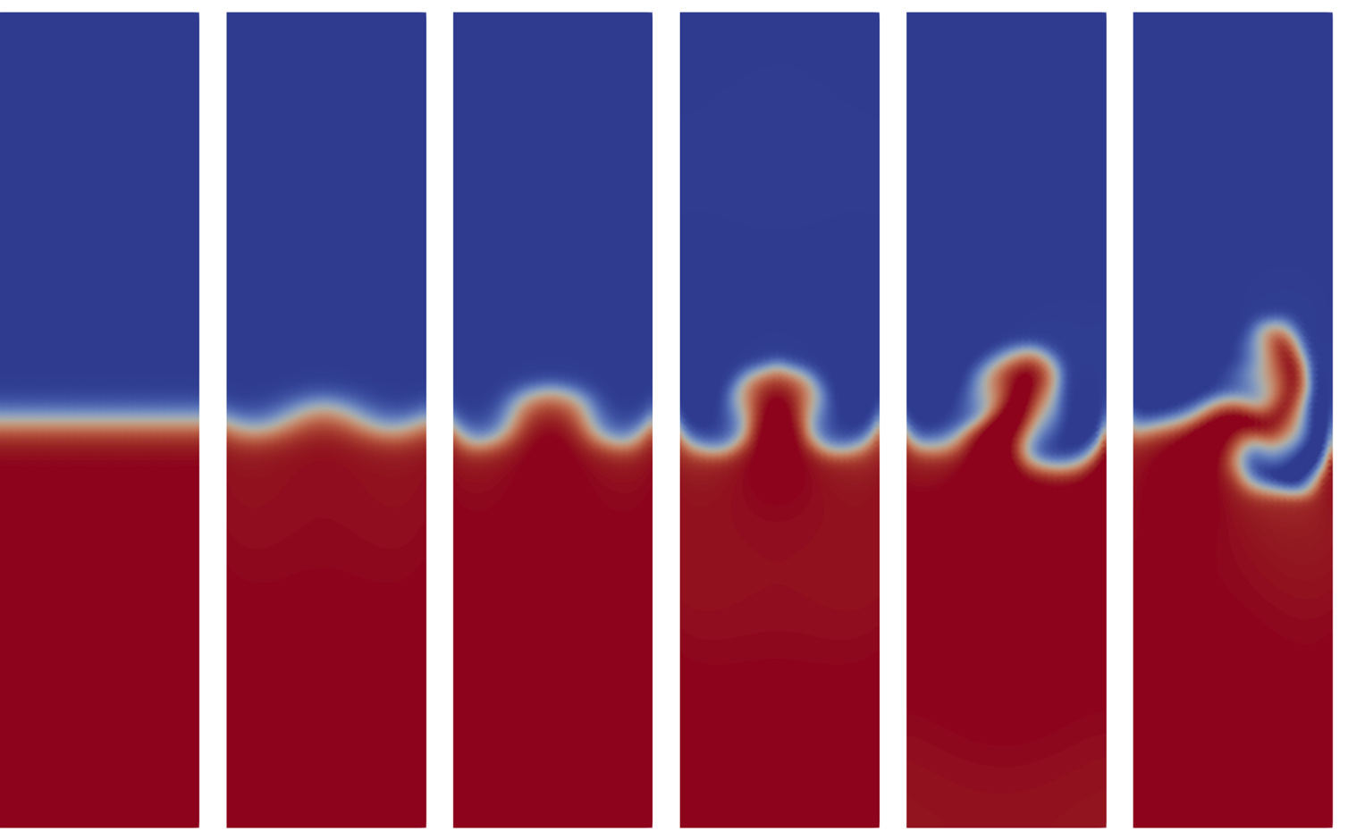
Next, we simulated a magnetic Rayleigh–Taylor instability on the domain $\varOmega = [0,L] \times [0,4L]$ with $L=\frac {1}{4}$. We chose

(5.2)\begin{equation} \epsilon(\rho,s) = K e^{s/(C_v \rho)} \rho^\gamma, \end{equation}

with $C_v=K=1$ and $\gamma =\frac {5}{3}$, and we set $\mu =\nu =\lambda =0.01$ and $\phi =-y$, which corresponds to an upward gravitational force. As initial conditions, we take

(5.3)\begin{equation} \left.\begin{array}{c@{}} \displaystyle \rho(x,y,0) = 1.5-0.5\tanh\left( \dfrac{y-0.5}{0.02} \right), \\ \displaystyle u(x,y,0)= \left( 0, -0.025\sqrt{\dfrac{\gamma p(x,y)}{\rho(x,y,0)}} \cos(8{\rm \pi} x) \exp\left( -\dfrac{(y-0.5)^2}{0.09}\right) \right), \\ \displaystyle s(x,y,0) = C_v\rho(x,y,0) \log\left( \dfrac{p(x,y)}{(\gamma-1)K\rho(x,y,0)^\gamma}\right), \\ B(x,y,0) = (B_0,0), \end{array}\right\} \end{equation}

where

(5.4)\begin{equation} p(x,y) = 1.5y + 1.25 + (0.25-0.5y) \tanh\left( \frac{y-0.5}{0.02} \right). \end{equation}

This system is known to exhibit instability when $B_0 < B_c= \sqrt {( \rho _h - \rho _l) gL}$, where here $\rho _h=2, \rho _l=1, g=1, L=1/4$, Chandrasekhar (Reference Chandrasekhar1961).

We imposed boundary conditions $u = (B-(B_0,0)) \cdot n = {\rm curl} B \times n = 0$ on $\partial \varOmega$. We triangulated $\varOmega$ with a uniform triangulation $\mathcal {T}_h$ having maximum element diameter $h=2^{-7}$, and we used the finite element spaces specified in § 3 of order $r=s=0$. We ran simulations from $t=0$ to $t=5$ using a time step $\Delta t = 0.005$. 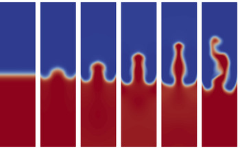Plots of the computed mass density for various choices of $B_0$ are shown in figures 2–5. The figures indicate that the scheme correctly predicts instability for $B_0< B_c=0.5$ (figures 2 and 3) and stability for $B_0>B_c=0.5$ (figures 4 and 5).

Figure 2.

Contours of the mass density at $t=0,1,2,3,4,5$ when $B_0=0.2$.

Figure 3.

Contours of the mass density at $t=0,1,2,3,4,5$ when $B_0=0.4$.

Figure 4.

Contours of the mass density at $t=0,1,2,3,4,5$ when $B_0=0.6$.

Figure 5.

Contours of the mass density at $t=0,1,2,3,4,5$ when $B_0=0.8$.

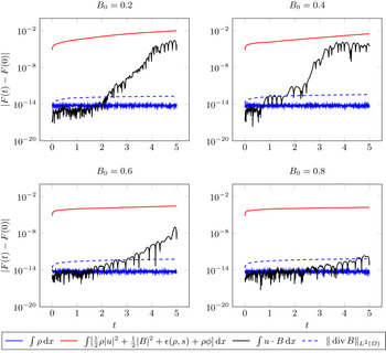
The evolution of energy, cross-helicity, mass and $\|{\rm div} B\|_{L^2(\varOmega )}$ during these simulations is plotted in figure 6. (Magnetic helicity is not plotted since it is trivially preserved in two dimensions if we take $A$ to be orthogonal to the plane.) As predicted by Proposition 4.1, figure 6 shows that energy decayed monotonically, while mass and ${\rm div} B = 0$ were preserved to machine precision. Interestingly, the cross-helicity drifted by less than $2.5 \times 10^{-4}$ in these experiments.

Figure 6.

Evolution of mass, energy, cross-helicity and $\|{\rm div} B\|_{L^2(\varOmega )}$ during simulations of the magnetic Rayleigh–Taylor instability with $B_0=0.2,0.4,0.6,0.8$. The absolute deviations $|F(t)-F(0)|$ are plotted for each such quantity $F(t)$.

Editor Emanuele Tassi thanks the referees for their advice in evaluating this article.