



1. Introduction
Rogue waves are extreme and highly localised events that pose significant risks to offshore structures and marine operations. They are characterised by an exceptionally large wave height, strong destructive power, highly concentrated energy, and significant nonlinearity (Dysthe et al. Reference Dysthe, Krogstad and Müller2008). Such waves appear and disappear without warning, posing a serious threat to coastal and offshore structures as well as vessels. Understanding and predicting these extreme events remains a significant scientific challenge, with direct implications for maritime safety and the design of coastal and offshore infrastructure.
There are numerous causes for the formation of freak waves. Kharif & Pelinovsky (Reference Kharif and Pelinovsky2003) systematically analysed the formation mechanisms of rogue waves, and suggested that their occurrence may result from energy focusing due to one or several factors, such as linear wave superposition, nonlinear modulation instability, bathymetric variations, wave–current interactions, and wind effects. One way to generate rogue waves in a laboratory environment is by the use of fundamental breather solutions in the form of a time-periodic, doubly localised and space-periodic Peregrine breather (PB) (Peregrine Reference Peregrine1983). The PB is an exact solution of the nonlinear Schrödinger equation (NLSE), and describes unidirectional modulational dynamics. Experiments observing this PB soliton have been performed in a water wave tank (Chabchoub et al. Reference Chabchoub, Hoffmann and Akhmediev2011), in optical fibres (Kibler et al. Reference Kibler, Fatome, Finot, Millot, Dias, Genty, Akhmediev and Dudley2010), and in plasmas (Bailung et al. Reference Bailung, Sharma and Nakamura2011). Recently, Liao et al. (Reference Liao, Ma and Liu2024) investigated the evolution of the PB under varying water depths and wave steepnesses experimentally and numerically, demonstrating that the high-order NLSE accurately captures asymmetric wave features and predicts a higher likelihood of freak waves in shallower water.
However, the scenarios examined above primarily involve rogue waves arising from a regular, monochromatic carrier wave – a condition rarely observed in the ocean. To bridge the gap towards practical oceanographic relevance, it is essential to investigate the dynamics of rogue waves in more complex background wave train conditions. Recent theoretical studies have extended rogue wave solutions from idealised plane wave backgrounds to structured wave environments. For instance, Ling & Sun (Reference Ling and Sun2024) established a quantitative correspondence between elliptic rogue waves and modulational instability on periodic backgrounds, demonstrating that modulational instability of elliptic waves can induce localised extreme events. Similarly, Chang & Zhaqilao (Reference Chang and Zhaqilao2025) constructed rogue wave solutions on Jacobian elliptic dn- and cn-periodic backgrounds for the Kraenkel–Manna–Merle system, and obtained a rogue wave on a skewed periodic wave background. Experimental (Chabchoub Reference Chabchoub2016) and numerical (Wang et al. Reference Wang, Ma, Yan and Chabchoub2018) studies verified that the PB can evolve into a rogue wave within a Joint North Sea Wave Project (JONSWAP) sea state. He et al. (Reference He, Slunyaev, Mori and Chabchoub2022b ) provided the first experimental demonstration that the PB can undergo nonlinear focusing in standing water waves, maintaining coherence and amplification even in the presence of a counterpropagating wave train, in agreement with the coupled NLSE. Liu et al. (Reference Liu, Feng and Cui2023) experimentally demonstrated that the PB solution can generate extreme waves under a random sea background, and revealed that characteristic triangular spectral features – observable in both first and second harmonics – persist and can serve as early indicators for extreme wave formation. Despite these advances, the influence of the statistical properties of the background wave field on rogue wave evolutions remains systematically unexplored.
This study aims to identify the physical mechanisms by which narrow-banded random background wave fields influence the evolution of PBs. We systematically vary three statistical parameters of the background wave fields – the peak wavenumber, the significant wave height and the spectral width – and analyse their influence on the PB, including the maximum crest height, the timing of rogue wave emergence, and the spatiotemporal distribution of rogue waves. To elucidate the underlying mechanisms, the surface profiles, amplitude spectra, phase perturbations, Benjamin–Feir index, and kurtosis during the evolution under different background wave fields are examined. The paper is organised as follows: § 2 describes the mathematical formulation and numerical set-up; § 3 presents the numerical results and discussion; and § 4 summarises the main conclusions.
2. Mathematical descriptions
We simulate the evolution of a two-dimensional irrotational, inviscid and incompressible gravity PB wave under the influence of narrow-banded background wave fields aligned with the propagation direction of the PB, in deep water using the pseudo-spectral Fourier–Legendre (PFL) method (Klahn et al. Reference Klahn, Madsen and Fuhrman2021b ). This method provides stable and accurate solutions for highly nonlinear waves (Klahn et al. Reference Klahn, Madsen and Fuhrman2020), which aligns well with the strong nonlinearity inherent in rogue wave development processes.
2.1. Governing equations
Let
 $z$
denote the vertical coordinate,
 $x$
the horizontal coordinate,
 $t$
the time,
 $z = \eta ( x, t )$
the free surface, and
 $\varPhi ( x, z, t )$
the velocity potential. The governing equations are
 \begin{align} \frac {\partial ^ 2 \varPhi }{\partial x ^ 2} + \frac {\partial ^ 2 \varPhi }{\partial z ^ 2} = 0,\:\:\: - h \lt z \lt \eta \left ( x, t \right ), \\[-28pt] \nonumber \end{align}
 \begin{align} \frac {\partial \varPhi }{\partial z} = 0,\:\:\: z = - h, \\[-28pt] \nonumber \end{align}
 \begin{align} \frac {\partial \eta }{\partial t} = \left ( 1 + \left ( \frac {\partial \eta }{\partial x} \right ) ^ 2 \right ) w_{{s}} - \frac {\partial \eta }{\partial x} \frac {\partial \varPhi _ {s}}{\partial x} + 2 \nu \frac {\partial ^ 2 \eta }{\partial x ^ 2}, \\[-28pt] \nonumber \end{align}
 \begin{eqnarray} \frac {\partial \varPhi _ {s}}{\partial t} = - g \eta - \frac {1}{2} \left ( \frac {\partial \varPhi _{{s}}}{\partial x} \right ) ^ 2 + \frac {1}{2} \left ( 1 + \left ( \frac {\partial \eta }{\partial x} \right ) ^ 2 \right ) w_{{s}}^2 + 2 \nu \frac {\partial ^ 2 \varPhi _{{s}}}{\partial x ^ 2}, \\[3pt] \nonumber \end{eqnarray}
where
 $w_{{s}} = \partial _z \varPhi |_{z = \eta }$
and
 $\varPhi _{{s}} = \varPhi | _{z = \eta }$
are the vertical velocity and velocity potential of the fluid at the free surface, respectively,
 $g = 9.81 \, \text{m}\,\text{s}^{-2}$
is the gravitational acceleration, and
 $h$
is the water depth. Dissipation effects due to wave breaking and non-breaking processes are incorporated via eddy viscosity terms
 $2 \nu ( \partial ^ 2 \eta / \partial x ^ 2 )$
and
 $2 \nu (\partial ^ 2 \varPhi _{{s}} / \partial x ^ 2 )$
(Tian et al. Reference Tian, Perlin and Choi2010). This eddy viscosity model is derived under the small-viscosity assumption from the viscous free-surface boundary conditions for weakly damped surface waves (Ruvinsky et al. Reference Ruvinsky, Feldstein and Freidman1991; Longuet-Higgins Reference Longuet-Higgins1992; Tian et al. Reference Tian, Perlin and Choi2010). The leading-order viscous effect is incorporated into the free-surface boundary conditions, and Longuet-Higgins (Reference Longuet-Higgins1992) suggested that the kinematic viscosity
 $ \nu$
can be replaced by an eddy viscosity
 $ \nu _{\textit{eddy}}$
to represent the energy dissipation due to wave breaking. To identify the onset of wave breaking, the kinematic breaking criterion proposed by Barthelemy et al. (Reference Barthelemy, Banner, Peirson, Fedele, Allis and Dias2018) is adopted. Once the breaking criterion is satisfied, the viscosity
 $ \nu$
is replaced by the eddy viscosity
 $ \nu _{\textit{eddy}}$
to account for the dissipation by wave breaking events. The value of
 $ \nu _{\textit{eddy}}$
depends on the breaking intensity and is influenced by factors such as wave steepness (Drazen et al. Reference Drazen, Melville and Lenain2008). However, owing to the limitations of the experimental conditions in quantifying wave breaking strength, a constant value
 $ \nu _{\textit{eddy}} = 1 \times 10^{-3} \, \text{m}^2\,\text{s}^{-1}$
, consistent with the order of magnitude proposed by Tian et al. (Reference Tian, Perlin and Choi2010), is adopted in the present study. For more details about the wave evolution model, please refer to Cheng et al. (Reference Cheng, Liu, Cui and Sun2025).
2.2. Initial conditions and computational parameters
In this study, we embed a PB into a random background wave field to investigate the influence of background wave fields on PB evolution. The surface elevation is expressed as
 \begin{align} \eta = \eta _{\textit{PB}} + \eta _{\textit{BG}}, \end{align}
where
 $ \eta _{\textit{PB}}$
and
 $ \eta _{\textit{BG}}$
denote the surface elevations of the PB and the background wave field, respectively.
Following Chabchoub et al. (Reference Chabchoub, Hoffmann and Akhmediev2011), the PB surface elevation is defined to first order of approximation as
 \begin{align} \eta _{\textit{PB}}(x, t)=\operatorname {Re}\{A_{{p}}(x, t) \exp [{\rm i}(k x-\omega t)]\}, \end{align}
with the dimensional form of the wave envelope
 $ A_{{p}}$
given by
 \begin{align} A_{{p}}(x, t)=a\left (-1+\frac {4\left (1-{\rm i}\alpha ^{2} \omega t\right )}{1+8 \alpha ^{2} k^{2}\left (x-c_{g} t\right )^{2}+\alpha ^{4} \omega ^{2} t^{2}}\right ) \exp \left (-\frac {{\rm i}\omega \alpha ^{2} t}{2}\right ) \!, \end{align}
where
 $ a$
is the carrier wave amplitude,
 $ k$
is the wavenumber,
 $ \omega$
is the angular frequency,
 $ \alpha = ka$
is the wave steepness, and
 $ c_g = \partial \omega / \partial k = \omega / ( 2 k )$
is the group velocity. The carrier wavenumber is fixed at
 $ k_p = 4 \pi \, \text{m}^{-1}$
, corresponding to wavelength
 $ \lambda _p = 0.5 \, \text{m}$
. The wave steepness is set to
 $ \alpha = 0.1$
, and the initial wave field is specified by
 $ \eta _{\textit{PB}} (x, t_0)$
, where
 $ t_0 = -40 \, \text{s}$
.
The background wave field is specified by a Gaussian wavenumber spectrum (Alber Reference Alber1978)
 \begin{align} W_{0}(p)=\frac {\left \langle a_{0}^{2}\right \rangle }{\sigma _{k} k_0 \sqrt {2 \pi }} \exp \left (-\frac {p^{2}}{2 \left ( \sigma _{k} k_0 \right )^{2}}\right ), \end{align}
where
 $ a_{0} = \langle \eta _{\textit{BG}}(x)^2 \rangle ^{1/2}$
is a constant envelope variance,
 $ k_0$
is the carrier wavenumber,
 $ p = k - k_0$
is the deviation from the carrier wavenumber, and
 $ \sigma _{k}$
is the relative spectral width. The background surface elevation is constructed via linear superposition of wave components with random phases,
 \begin{align} \eta _{\textit{BG}}(x, t)=\sum _{n=1}^{N} a_{n} \cos (k_{n} x-\omega _{n} t+\varphi _{n}), \end{align}
with amplitudes
 \begin{align} a_{n}=\sqrt {2 W_0 (k_{n} - k_0)\, \Delta k}, \end{align}
where
 $ \varphi _n$
is randomly distributed in
 $ [ 0, 2 \pi )$
. Here,
 $k_n$
is the wavenumber of the
 $ n \text{th}$
component,
 $N$
is the total number of wave components, and
 $ \Delta k$
denotes the wavenumber interval.
In the computation set-up, we define the computational domain as
 $x \in [ 0, 50 ]\ \text{m}$
, and the vertical extent of the fluid domain is reduced by using the artificial boundary condition with
 $b ( t ) = 1.2 \max \left | \eta ( x, t ) \right |$
. Simulations utilise
 $ 2^{12}$
horizontal grid points such that the carrier wave field is resolved by
 $ \lambda _0 / \Delta x \gt 40$
points per wavelength, coupled with
 $21$
points distributed in the vertical direction. The time step is
 $0.02T_p$
, where
 $T_p$
is the peak wave period. Following Klahn et al. (Reference Klahn, Madsen and Fuhrman2021a
), starting with linearised initial conditions, the nonlinear terms are ramped to full on over duration
 $ 1 T_p$
. Simulations then continue for total duration
 $ 130 T_p$
to avoid the impact of periodic boundary conditions.
For algorithm stability, the same artificial damping as used in Cheng et al. (Reference Cheng, Liu, Cui and Sun2025) is applied during the evolution, and the filter parameter is set to
 $ 0.6$
.
3. Results and discussion
3.1. Validation and definition of abnormality indices
We first validated the applicability of the PFL method for simulating PB evolution by reproducing the experiment of He et al. (Reference He, Ducrozet, Hoffmann, Dudley and Chabchoub2022a
), with details presented in Appendix A. After validation, we simulate PB evolution with kinematic viscosity
 $ \nu = 1.0067 \times 10^{-6} \, \text{m}^2\,\text{s}^{-1}$
, as this study focuses on the PB solution in the open-sea state. A rogue wave is commonly defined by the criterion
 $ \eta _c / H_s \gt 1.25$
, where
 $ \eta _c$
denotes the crest wave height, and
 $H_s = 4 \left \langle \eta ^ 2 \right \rangle ^ {1/2}$
is the significant wave height. This criterion is first satisfied at
 $ t = 82.96 \, T_p$
, and the maximum value of
 $ \eta _c / H_s$
is reached at
 $ t = 87.1 \, T_p$
.
After the standard case of PB evolution, the effects of the background wave fields on the evolution of PB can now be explored. The parameters of the PB wave are shown in § 2.2, while the range of the parameters of background wave fields needs to be properly selected. We investigate the influence of background wave fields on PB evolution by varying three parameters: the peak wavenumber
 $ k_{p,\textit{BG}}$
, the significant wave height
 $ H_{s,{BG}}$
, and the relative width of the spectrum in wavenumber space
 $ \sigma _{k}$
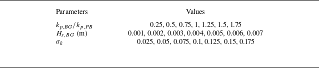
. The primary parameter ranges are summarised in table 1. For
 $ H_{s,{BG}}$
, the effects of the background wave field on the PB are negligible when its significant height is too small. However, when the background significant wave height becomes excessively large, the PB signature is weakened. Since the
 $H_{s}$
of the PB is approximately
 $ 0.0225 \, \text{m}$
, we set the background wave field within a range
 $ 0.001 \le H_{s,{BG}} \le 0.007 \, \text{m}$
. In addition, to examine the influence of spectral width, additional simulations are performed with fixed
 $k_{p,\textit{BG}}=0.65k_{p,\textit{PB}}$
and
 $1.4k_{p,\textit{PB}}$
, and
 $H_{s,{BG}}=0.004\,\mathrm{m}$
, by varying
 $\sigma _k$
.
Parameter ranges for the Gaussian background wave field. The peak wavenumber
 $ k_{p,\textit{BG}}$
is normalised by the PB carrier wavenumber
 $ k_{p, \textit{PB}} = 4 \pi \, \text{m}^{-1}$
; the significant wave height
 $ H_{s,{BG}}$
is given in metres; and the spectral width
 $ \sigma _k$
denotes the relative width of the Gaussian spectrum in wavenumber space.

Table 1. Long description
A table with three columns and three rows detailing parameter ranges for a Gaussian background wave field. The columns are labeled Parameters, k_BG/k_PB, H_s,BG (m), and σ_k. The row values are as follows: Row 1: Parameters, k_BG/k_PB, H_s,BG (m), σ_k; Row 2: Values, 0.25, 0.5, 0.75, 1, 1.25, 1.5, 1.75, 0.001, 0.002, 0.003, 0.004, 0.005, 0.006, 0.007, 0.025, 0.05, 0.075, 0.1, 0.125, 0.15, 0.175.
To characterise the behaviour of the PB with background waves, two abnormality indices are introduced, following definitions similar to those adopted in a previous study (Wang et al. Reference Wang, Ma, Yan and Chabchoub2018). These indices quantify the intensity and the occurrence time of rogue wave events, respectively:
 \begin{align} I_{A}=\max \left (\eta _{c}(x, t / T_p) / H_{s}\right ), \\[-28pt] \nonumber \end{align}
 \begin{align} I_{F}=T_{F} / T_{F, 0}, \\[-12pt] \nonumber \end{align}
where
 $ T_{F}$
is the first time a rogue wave is detected during the evolution, and
 $ T_{F, 0} = 82.96 \, T_p$
denotes the corresponding time of the PB without the background wave field. A schematic illustration of
 $ I_A$
and
 $ I_F$
is provided in figure 1.
Schematic illustration of the abnormality indices
 $ I_A$
and
 $ I_F$
, where
 $ I_A$
is defined as the maximum wave height, and
 $ I_F$
represents the time of the first occurrence of a rogue wave. The fixed position
 $ x = 30.36 \, \text{m}$
in (a) corresponds to the spatial location of the maximum
 $ I_A$
, while the symbols
 $ x_{T_F}$
and
 $ x_{T_{F, 0}}$
in (b) denote the crest positions at
 $ t = T_F$
and
 $ T_{F, 0}$
, respectively.

Before further analysis, the investigation of the effects of random phases is performed. The convergence analysis regarding the number of realisations is detailed in Appendix B, and we use
 $ 20$
realisations in this study.
3.2. Effect of background peak wavenumber
Figure 2 presents the variations of
 $I_A$
and
 $ I_F$
with respect to
 $k_{p,\textit{BG}}$
for
 $ H_{s,{BG}} = 0.004 \, \text{m}$
and
 $ \sigma _k = 0.1$
. Rogue waves are observed in all cases. When the peak wavenumber of the background wave field matches that of the PB, the wave system reaches a higher
 $ \eta _c$
, resulting in an average
 $ 4.4 \,\%$
increase in
 $ I_A$
relative to the PB-only case. When
 $ k_{p, \textit{BG}} = 0.75 k_{p, \textit{PB}}$
and
 $ 1.25 k_{p, \textit{PB}}$
,
 $ I_A$
is slightly reduced relative to the case without background waves. As
 $ k_{p, \textit{BG}}$
deviates further from
 $ k_{p, \textit{PB}}$
, the effect of the background wave field on PB evolution becomes negligible. Regarding the occurrence time, the rogue wave appears earlier when
 $ k_{p,\textit{BG}} = k_{p,\textit{PB}}$
, corresponding to an average reduction of
 $ 15.9 \,\%$
in
 $ I_F$
, equivalent to an earlier rogue wave occurrence by
 $ 13.2 \, T_p$
approximately. For
 $ k_{p,\textit{BG}} = 0.75 k_{p,\textit{PB}}$
and
 $ k_{p,\textit{BG}} = 1.25 k_{p,\textit{PB}}$
, the average first rogue wave occurrence is delayed by approximately
 $ 11.8 \,\%$
and
 $ 3.65 \,\%$
, respectively. The delay diminishes as
 $ k_{p,\textit{BG}}$
deviates further away from the PB carrier wavenumber. Overall, the influence of the background wave field on PB evolution becomes more pronounced as the background peak wavenumber approaches that of the PB, while the effect is negligible when the deviation is sufficiently large.
Plots of (a)
 $I_A$
and (b)
 $ I_F$
with respect to
 $k_{p,\textit{BG}}$
for
 $ H_{s,{BG}} = 0.004 \, \text{m}$
and
 $ \sigma _k = 0.1$
. Violin plots depict the distributions of
 $I_A$
and
 $ I_F$
for the corresponding dimensionless ratio of
 $ k_{p,\textit{BG}}$
relative to
 $ k_{p,\textit{PB}}$
. The horizontal blue dashed lines represent the corresponding parameters of PB without the background wave field.

Figure 3 presents the average wavenumber spectra over
 $ 20$
realisations for
 $ k_{p,\textit{BG}} = 0.75 k_{p,\textit{PB}}$
and
 $ k_{p,\textit{BG}} = k_{p,\textit{PB}}$
, at three characteristic instants:
 $ t = 0$
,
 $ t = T_F / 2$
and
 $ t = T_F$
. At
 $ t = 0$
, the peak wavenumber of both cases is
 $ k_p = 4\pi \, \text{m}^{-1}$
, with additional energy contributions from the background wave fields. As the system evolves to
 $ t = T_F / 2$
, the wave energy is transferred from the carrier wave to sideband wave components. For
 $ k_{p,\textit{BG}} = k_{p,\textit{PB}}$
, the wave energy is concentrated around the carrier wave, whereas for
 $ k_{p,\textit{BG}} = 0.75 k_{p,\textit{PB}}$
, the wave energy is transferred from the carrier wave to a broader range of wave components. At
 $ t = T_F$
, the distinction between these two cases becomes more evident. When
 $ k_{p,\textit{BG}} = k_{p,\textit{PB}}$
, the spectral energy remains concentrated near the carrier wave, facilitating stronger nonlinearity. In contrast, for
 $ k_{p,\textit{BG}} = 0.75 k_{p,\textit{PB}}$
, more wave energy is transferred from the carrier to the sidebands. These results explain the trend observed in figure 2(b): when the background peak wavenumber deviates from the PB carrier, more carrier energy is diverted to sideband components than when
 $ k_{p,\textit{BG}} = k_{p,\textit{PB}}$
, prolonging the nonlinear energy transfer process. Consequently, the rogue wave emerges later than in the case where
 $ k_{p, \textit{BG}} = k_{p, \textit{PB}}$
.
Average wavenumber spectrum for (a–c)
 $k_{p,\textit{BG}} = 0.75 k_{p, \textit{PB}}$
and (d–f)
 $k_{p,\textit{BG}} = k_{p, \textit{PB}}$
over
 $ 20$
realisations at
 $t = 0$
,
 $t = T_F / 2$
and
 $t = T_F$
. The initial spectrum consists of both the PB and the background wave field.

Given that the PB is a nonlinearity-driven rogue wave system (He et al. Reference He, Slunyaev, Mori and Chabchoub2022b
), modulation instability – recognised as a key mechanism for rogue wave formation – is characterised by the Benjamin–Feir index (BFI) (Janssen Reference Janssen2003). Waves are found to be stable to sideband perturbations when
 $ \text{BFI} \lt 1$
, and the definition of BFI is given by
 \begin{align} \text{BFI} = \frac {\epsilon }{\sqrt {2}\, \delta _{\omega }} = \frac {a_0 k_p}{\sqrt {2}\, \delta _{\omega }}, \end{align}
where
 $ \epsilon$
is spectral steepness,
 \begin{align} a_0 = \frac {H_s}{2} = 2 \sqrt {m_0} \end{align}
is the wave amplitude,
 \begin{align} m_n = \int_{0}^{\infty } \omega ^n\, S ( \omega )\, \text{d} \omega \end{align}
is the
 $n$
th spectral moment,
 \begin{align} \delta _\omega = \frac {1}{Q_p\, \sqrt { \pi }} \end{align}
is the bandwidth defined by Serio et al. (Reference Serio2005) for the discrete spectrum, and
 \begin{align} Q_p = \frac {2}{m_0^2} \int \omega\, S^2 ( \omega )\, \text{d} \omega \end{align}
is Goda’s peakedness parameter. Figure 4 illustrates the temporal evolution of the average BFI and kurtosis over
 $ 20$
realisations for different
 $ k_{p, \textit{BG}}$
, together with the corresponding energy distribution among different wavenumber ranges. As shown in figure 4(a), for
 $ k_{p, \textit{BG}} = 0.75 k_{p, \textit{PB}}, k_{p, \textit{PB}}, 1.25 k_{p, \textit{PB}}$
, the BFI decreases with time, indicating continuous spectral broadening and strong modulational instability. In contrast, when
 $ k_{p, \textit{BG}}$
deviates further away from
 $ k_{p, \textit{PB}}$
, the BFI initially decreases and then increases. This non-monotonic behaviour indicates that nonlinear interactions initially broaden the spectrum, after which a redistribution of wave energy narrows it, resulting in an increased BFI. Among all cases, the most rapid decrease in BFI is observed when
 $ k_{p, \textit{BG}} = k_{p, \textit{PB}}$
. The evolution of kurtosis is presented in figure 4(b). For
 $ k_{p, \textit{BG}} = 0.75 k_{p, \textit{PB}}, k_{p, \textit{PB}}, 1.25 k_{p, \textit{PB}}$
, the kurtosis remains higher than in the other cases during the evolution, corresponding to a higher probability of rogue wave events (Janssen Reference Janssen2003). Figure 4(c) shows the evolution of energy fractions distributed across different wavenumber ranges, where
 $ \varPi$
denotes the sum of the squared amplitudes of all wave components, and
 $ \varPi _1$
,
 $ \varPi _2$
and
 $ \varPi _3$
represent the sums of squared amplitudes for components with wavenumbers
 $ k \lt k_{p, \textit{PB}}$
,
 $ k = k_{p, \textit{PB}}$
and
 $ k \gt k_{p, \textit{PB}}$
, respectively. Under the matched condition (
 $ k_{p, \textit{BG}} = k_{p, \textit{PB}}$
), wave energy is transferred faster from the carrier wave to sideband wave components, indicating more efficient energy exchange and stronger modulational instability.
Evolution of (a) the BFI, and (b) kurtosis for different
 $ k_{p,\textit{BG}}$
. (c) Time evolution of the energy fractions divided into three parts –
 $ \varPi _1$
(wavenumbers
 $ k \lt k_{p, \textit{PB}}$
),
 $ \varPi _2$
(
 $ k = k_{p, \textit{PB}}$
) and
 $ \varPi _3$
(wavenumbers
 $ k \gt k_{p, \textit{PB}}$
) – for
 $ k_{p, \textit{BG}} = 0.75 k_{p, \textit{PB}}, k_{p, \textit{PB}}, 1.25 k_{p, \textit{PB}}$
. Results are averages over
 $ 20$
realisations.

Figure 4. Long description
Panel A: A line graph shows the evolution of the Benjamin-Feir index (BFI) over time (t/T_P) for different values of k_p,BG. The x-axis represents time (t/T_P) and the y-axis represents BFI. The legend indicates different values of k_p,BG ranging from 0.25k_p,PB to 1.75k_p,PB. The lines show a general trend of decreasing BFI over time for all values of k_p,BG. Panel B: A line graph shows the evolution of kurtosis over time (t/T_P) for different values of k_p,BG. The x-axis represents time (t/T_P) and the y-axis represents kurtosis. The legend indicates different values of k_p,BG ranging from 0.25k_p,PB to 1.75k_p,PB. The lines show an increasing trend in kurtosis over time for all values of k_p,BG. Panel C: Multiple line graphs show the time evolution of energy fractions divided into three parts (wavenumbers 1, 2, and 3) for different values of k_p,BG. The x-axis represents time (t/T_P) and the y-axis represents the percentage of energy. The legend indicates different values of k_p,BG and the corresponding energy fractions. The lines show varying trends in energy fractions over time for different values of k_p,BG.
The average wave spectra at the moment of maximum
 $ I_A$
under different
 $ k_{p, \textit{BG}}$
are shown in figure 5. For
 $ k_{p, \textit{BG}} = 0.75 k_{p, \textit{PB}}, k_{p, \textit{PB}}, 1.25 k_{p, \textit{PB}}$
, the amplitude of the carrier wave component (
 $ k = 4 \pi \, \text{m}^{-1}$
) is significantly smaller than in both the PB-only case and cases with other
 $ k_{p, \textit{BG}}$
. This indicates that when the background peak wavenumber
 $ k_{p, \textit{BG}}$
is close to the PB carrier wavenumber, wave energy is concentrated around the carrier at the initial time, promoting stronger nonlinear interactions and more efficient energy transfer from the carrier to the sidebands. As a result, the wave energy is more broadly distributed across the wavenumber spectrum at the moment of maximum
 $ I_A$
, and the strongest effect is under the matched condition
 $ k_{p, \textit{BG}} = k_{p, \textit{PB}}$
.
Comparison of wave spectra at the moment of maximum
 $ I_A$
for (a)
 $ k_{p, \textit{BG}} = 0.5 k_{p, \textit{PB}}, 0.75 k_{p, \textit{PB}}, k_{p, \textit{PB}}$
and the PB-only case, and (b)
 $ k_{p, \textit{BG}} = k_{p, \textit{PB}}, 1.25 k_{p, \textit{PB}}, 1.5 k_{p, \textit{PB}}$
and the PB-only case. Each spectrum represents the average over
 $ 20$
realisations.

Figure 6 presents the spatiotemporal distributions of rogue wave occurrence. At each discrete point in space and time, the value
 $ N (t, x)$
is the average fraction over
 $ 20$
realisations that satisfy the rogue wave criterion, providing a statistical measure of rogue wave occurrence likelihood. During the evolution of the PB without background wave fields (figure 6
a), rogue waves appear intermittently within the spatiotemporal domain
 $ x \in [ 29.14, 32.4 ] \ \text{m}, \ t \in [ 82.96, 95.3 ] \, T_p$
. For
 $ k_{p, \textit{BG}} \le 0.5 k_{p, \textit{PB}}$
, compared with the benchmark case in figure 6(a), rogue waves are detected in an expansion of the original spatiotemporal region. As the background peak wavenumber approaches the PB carrier, rogue waves are observed over an extended region, and emerge in additional spatiotemporal regions. When
 $ k_{p, \textit{BG}} = k_{p, \textit{PB}}$
, a significant increase in the number of spatiotemporal locations satisfying the rogue wave criterion is observed. This suggests a broader spatiotemporal distribution of rogue wave occurrence when the background peak wavenumber matches that of the PB. However, as
 $ k_{p, \textit{BG}}$
continues to increase beyond the carrier (i.e.
 $ k_{p, \textit{BG}} \gt k_{p, \textit{PB}}$
), the spatiotemporal distribution of rogue waves becomes less extensive, and the pattern progressively returns to that observed in the PB evolution without a background wave field.
Spatiotemporal distribution of rogue waves under (a) no background wave conditions and (b–h) different
 $ k_{p, \textit{BG}}$
. For cases with the background wave field, the results are averaged over
 $ 20$
realisations.

Figure 6. Long description
The image contains eight scatter plots showing the spatiotemporal distribution of rogue waves under various conditions. Each plot has the horizontal axis labeled as t/Tp and the vertical axis labeled as x (m). The color bar on the right represents the normalized intensity N(t,x), ranging from 0 to 1. Panel A shows the distribution without a background wave field. Panels B through H display the distribution with different background wave fields, with the wave number ratio kp,BG/kp,PB varying from 0.25 to 1.75. Each panel illustrates how the presence and intensity of the background wave field affect the distribution and intensity of rogue waves over time and space.
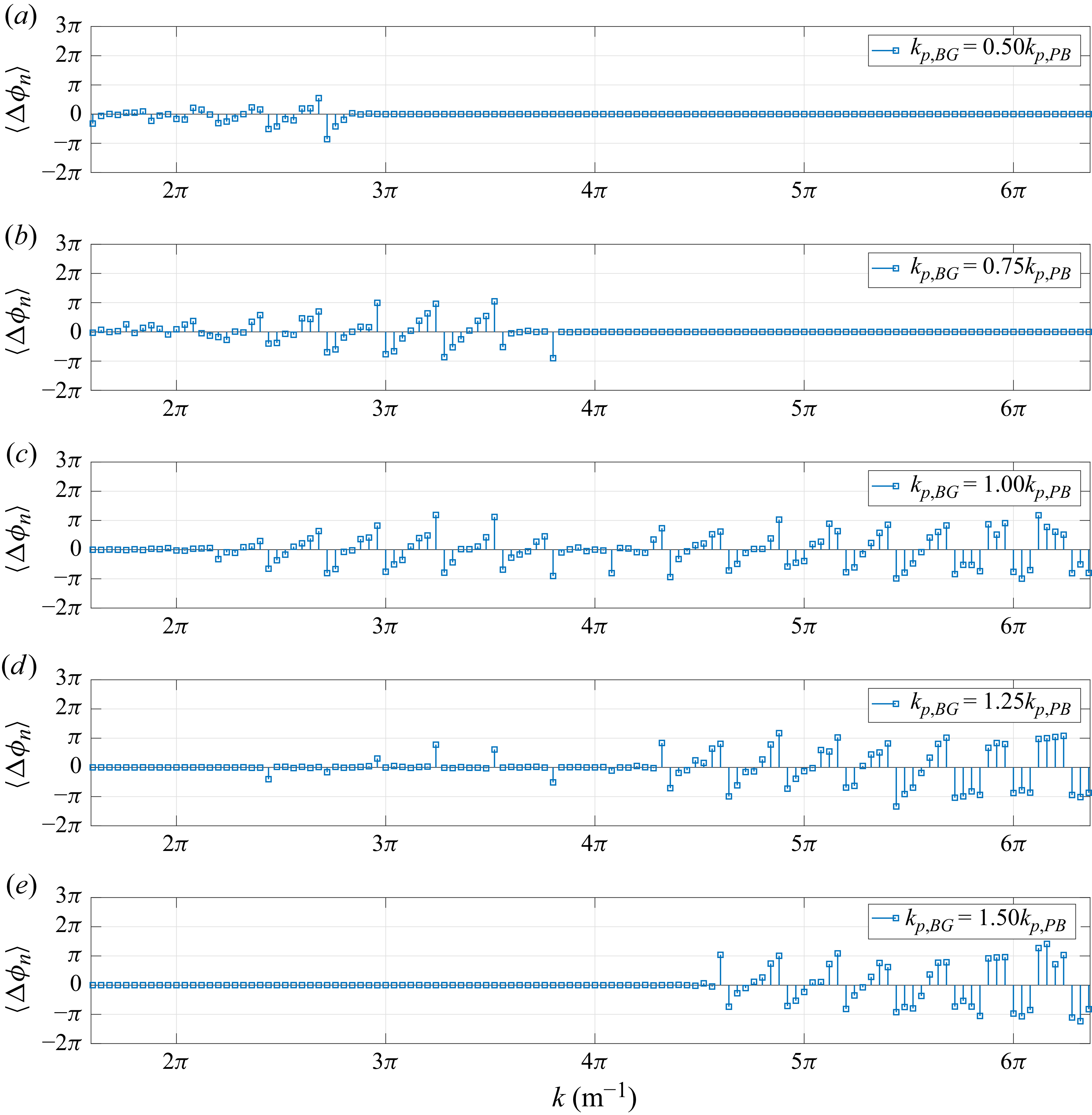
To further elucidate the mechanism responsible for the variation in the spatial distribution of rogue waves, figure 7 presents the phase perturbations induced by different background wave fields. The modification of the phase structure is quantified by the phase perturbation of the
 $n$
th wave component, defined as
 \begin{align} \Delta \phi _n = \phi _n(\mathrm{PB+BG}) - \phi _n(\mathrm{PB}), \end{align}
where
 $ \phi _n(\mathrm{PB+BG})$
and
 $ \phi _n(\mathrm{PB})$
denote the phases of the
 $n$
th wave component in the combined wave field and the PB-only case, respectively. For
 $ k_{p, \textit{BG}} = 0.5 k_{p, \textit{PB}}$
and
 $ 0.75 k_{p, \textit{PB}}$
, the phase perturbations are mainly distributed on the lower-wavenumber side of the carrier, whereas for
 $ k_{p, \textit{BG}} = 1.25 k_{p, \textit{PB}}$
and
 $ 1.5 k_{p, \textit{PB}}$
, the phase perturbations are more pronounced on the higher-wavenumber side. When
 $ k_{p, \textit{BG}} = k_{p, \textit{PB}}$
, the phase perturbations are concentrated around the carrier wavenumber, where the modulational instability is strongest. These phase perturbations modify the relative phase relationships among wave components, thereby affecting the phase-focusing process.
Mean phase perturbations at
 $ t = 0$
for different
 $ k_{p, \textit{BG}}$
and the PB-only case. The results are averaged over
 $ 20$
realisations.

The strongest rogue wave enhancement occurs when the peak wavenumber of the background field matches the carrier wavenumber of the PB (
 $ k_{p, \textit{BG}} = k_{p, \textit{PB}}$
). Under this condition, the total wave energy remains highly concentrated around the carrier wavenumber (figure 3
d), leading to stronger nonlinearity and more efficient nonlinear focusing (figure 4
c). In contrast, when the background peak wavenumber deviates from the PB carrier wavenumber (e.g.
 $ k_{p, \textit{BG}} = 0.75 k_{p, \textit{PB}}$
, figure 3
a), part of the wave energy is distributed among sideband wave components. This disperses the nonlinear interactions and prolongs the focusing process, resulting in a delayed occurrence of rogue waves. Since the background wave energy is much smaller than that of the PB, the background wave field can be regarded as a small perturbation to the PB. According to the classical Benjamin–Feir instability theory (Benjamin & Feir Reference Benjamin and Feir1967), sideband perturbations are unstable when
 $ 0 \lt \delta \lt \sqrt {2}\, k a$
, where
 $ \delta$
denotes the relative frequency deviation from the carrier wave. For the present initial PB steepness (
 $ ka = 0.1$
), the instability threshold is
 $ \delta _c \approx 0.141$
. Based on the linear dispersion relation in deep water,
 $ \delta _c$
corresponds to a Benjamin–Feir unstable wavenumber range approximately
 $ [ 0.74, 1.30 ] \, k_{p, \textit{PB}}$
. Both
 $ k_{p, \textit{BG}} = 0.75 k_{p, \textit{PB}}$
and
 $ k_{p, \textit{BG}} = 1.25 k_{p, \textit{PB}}$
fall within the unstable range, indicating that these two cases can enhance modulational instability. However, the enhancement is weaker than that under the perfectly matched condition (
 $ k_{p, \textit{BG}} = k_{p, \textit{PB}}$
), where the background-wave energy is concentrated directly around the carrier wavenumber. In addition, the phase perturbations (figure 7) reveal substantial phase modifications around the carrier wavenumber, which is the region where modulational instability is strongest. These phase perturbations alter the relative phase relationships among sideband wave components, creating additional opportunities for phase focusing, which makes rogue waves occur over a broader spatiotemporal distribution, consistent with the occurrence spatiotemporal region shown in figure 6. To further demonstrate that the observed spectral and phase perturbation characteristics are not averaging artefacts, representative results from individual realisations are provided in Appendix C, where consistent trends can be observed.
It is worth noting that among the
 $ 20$
independent realisations for
 $k_{p,\textit{BG}} = k_{p, \textit{PB}}$
,
 $ H_{s,{BG}} = 0.004 \, \text{m}$
and
 $ \sigma _k = 0.1$
, eight cases exhibit two rogue waves occurring simultaneously at distinct spatial locations, indicating that variations in the phase distribution can trigger multiple, spatially localised extreme events within the same wave field. To assess the robustness of this phenomenon and investigate the influence of model formulation, one representative realisation is selected and further simulated using the modified NLSE (MNLSE) (Trulsen et al. Reference Trulsen, Kliakhandler, Dysthe and Velarde2000) with the same initial condition as the PFL method. Compared with the NLSE, the MNLSE incorporates higher-order corrections and provides a more accurate description of nonlinear wave evolution. Figure 8 compares the surface profiles obtained from the PFL and MNLSE approaches at different times. The two methods show great agreement, indicating that both models capture the main characteristics of the nonlinear wave evolution process. However, the simultaneous occurrence of two rogue waves observed in the PFL simulation is not reproduced by the MNLSE at the corresponding time, as shown in figure 9. Although the MNLSE also captures a similar double-peak structure, the two peaks do not satisfy the rogue wave criterion due to the lower crest elevations predicted by the MNLSE compared with the PFL method. To clarify the mechanism underlying this discrepancy, figure 10 presents the evolution of wave spectra obtained from the two methods at different times. Although the overall spectral evolution is similar, the difference arises from the limited high-order bound-wave contributions in the MNLSE, which weaken wave steepening and crest amplification. Consequently, the simultaneous rogue wave event observed in the PFL simulation is not captured by the MNLSE. For completeness, the spatiotemporal evolution of the two rogue waves and the wave-envelope structures obtained by the PFL method are provided in Appendix D. Overall, these results demonstrate that the background wave field significantly modifies both the appearance time and the spatial distribution of rogue waves, with the strongest effect occurring when its peak wavenumber is equal to the PB carrier.
Comparisons of surface profiles obtained from the PFL and MNLSE approaches at different times during nonlinear wave evolution. The two simulations use the same initial condition.

Figure 8. Long description
The image contains six line graphs labeled (a) through (f), each showing surface profiles over a horizontal distance of 50 meters. The vertical axis represents the surface elevation (η) ranging from -0.02 to 0.02 meters. Each graph compares two datasets: PFL (solid blue line) and MNLSE (dashed red line). Panel (a) shows the initial condition at t = 0. Panels (b) through (f) display the surface profiles at different times during nonlinear wave evolution: t = 26Tp, t = 52Tp, t = 78Tp, t = 104Tp, and t = 130Tp, respectively. The graphs illustrate how the surface profiles evolve over time, with both datasets starting from the same initial condition. The PFL and MNLSE approaches show similar trends but with slight variations in the surface profiles as time progresses.
Comparison of free-surface profiles obtained from the PFL method and MNLSE at the time when two rogue waves occur simultaneously in the PFL simulation. The horizontal red dotted line indicates the rogue wave criterion
 $ \eta _c / H_s = 1.25$
.

Evolution of wave spectra predicted by the PFL and MNLSE approaches during nonlinear wave evolution.

Figure 10. Long description
Six line graphs depict the evolution of wave spectra over time. Panel A: At time t = 0, the graph shows a peak at around 5π m^-1 with values reaching approximately 8 x 10^-3. Panel B: At time t = 26Tp, the peak remains at around 5π m^-1 with similar values. Panel C: At time t = 52Tp, the peak is still at around 5π m^-1 with values around 8 x 10^-3. Panel D: At time t = 78Tp, the peak shifts slightly left and the values decrease. Panel E: At time t = 104Tp, the peak shifts further left and the values continue to decrease. Panel F: At time t = 130Tp, the peak is more spread out and the values are lower. Each graph has the x-axis labeled as k (m^-1) ranging from π to 13π and the y-axis labeled as <a> ranging from 0 to 8 x 10^-3. The legend indicates two data series: PFL in blue and MNLS in orange.
Although the present simulations are conducted at laboratory scale (
 $ \lambda _p = 0.5 \, \text{m}$
), the dominant mechanisms identified in this study – modulational instability, nonlinear focusing, and the nonlinear interaction between the PB and the background wave field – are governed primarily by non-dimensional parameters, including wave steepness, spectral bandwidth, and the relative relationship between the peak wavenumbers of the PB and the background wave field. Therefore, the physical mechanisms revealed here are expected to remain relevant in full-scale oceanic environments. In particular, the strongest enhancement of rogue wave events occurs when the peak wavenumber of the background wave field matches that of the PB (
 $ k_{p, \textit{BG}} = k_{p, \textit{PB}}$
). This finding implies that for well-known rogue wave events such as the Draupner wave (Haver Reference Haver2004), the Yura wave (Mori et al. Reference Mori, Liu and Yasuda2002) and the Pacific typhoon rogue wave (Mori et al. Reference Mori, Waseda and Chabchoub2023), a background sea state with a dominant wavenumber close to that of the extreme-wave group may provide favourable conditions for larger crest heights and a broader spatiotemporal distribution of rogue wave occurrence.
3.3. Background significant wave height
Figure 11 shows the variations of
 $I_A$
and
 $ I_F$
versus
 $H_{s,{BG}}$
for
 $ k_{p,\textit{BG}} = k_{p,\textit{PB}}$
and
 $ \sigma _k = 0.1$
. Here,
 $ I_A$
increases with
 $H_{s,{BG}}$
, then reaches a plateau, remaining at an average increase of approximately
 $ 5.4 \,\%$
for
 $H_{s,{BG}} \ge 0.004 \, \text{m}$
, indicating that increasing background wave energy enhances nonlinear interactions and strengthens maximum crest amplification until a saturation level is reached. Also,
 $ I_F$
decreases progressively with increasing
 $H_{s,{BG}}$
, reaching a maximum reduction of approximately
 $ 40.4 \,\%$
, implying that rogue waves appear earlier as the background wave field strengthens the nonlinear interactions. For each parameter combination, we generate 20 independent realisations with random phase distributions. Therefore, even identical parameter combinations may exhibit different violin distributions, reflecting the statistical variability induced by the random background wave fields.
Plots of (a)
 $I_A$
and (b)
 $ I_F$
with respect to
 $ H_{s,{BG}}$
for
 $k_{p,\textit{BG}} = k_{p, \textit{PB}}$
and
 $ \sigma _k = 0.1$
. Violin plots depict the distributions of
 $I_A$
and
 $ I_F$
for the corresponding
 $ H_{s,{BG}}$
. The horizontal blue dashed lines represent the corresponding parameters of PB without the background wave field.

The spatiotemporal distributions of rogue wave occurrence for different
 $ H_{s, \textit{BG}}$
are shown in figure 12. For
 $ H_{s,{BG}} = 0.001 \, \text{m}$
, the background wave field has a weak influence on PB, and rogue waves appear intermittently within a relatively confined region, similar to the PB-only case. As
 $ H_{s,{BG}}$
increases, the wave energy is more broadly distributed across the wavenumber spectrum (as shown in figure 13
a), thus rogue waves are detected over a more extended spatiotemporal distribution relative to the PB-only case. Meanwhile, as the background wave field becomes stronger, its influence on the phases of wave components near the carrier – where modulational instability is strongest – becomes more significant, as shown in figures 13(b–e). Enhanced variations in relative phase relationships lead to a broader spatiotemporal region of rogue wave occurrence. For larger
 $ H_{s,{BG}}$
, these effects become more pronounced: rogue waves occur earlier and may appear over an even wider spatiotemporal domain, reflecting the combined effects of strengthened nonlinear interactions and stronger variations in relative phase relationships. Overall, these results indicate that increasing the background wave height systematically enhances the nonlinear focusing process, thereby promoting both the intensity and the spatiotemporal prevalence of rogue waves.
Spatiotemporal distributions of rogue waves under different
 $ H_{s, \textit{BG}}$
. The results are averages over
 $ 20$
realisations.

(a) Comparison of wave spectra at the moment of maximum
 $ I_A$
for different
 $ H_{s, \textit{BG}}$
and the PB-only case. (b–e) Comparisons of the mean phase perturbations at
 $ t = 0$
for different
 $ H_{s, \textit{BG}}$
and the case of PB without background wave fields. The results are averaged over
 $ 20$
realisations.

3.4. Background spectral width
The variations of
 $I_A$
with respect to
 $\sigma _k$
for
 $ H_{s, \textit{BG}} = 0.004 \, \text{m}$
and
 $ k_{p,\textit{BG}} = 0.65 k_{p,\textit{PB}}$
,
 $ k_{p,\textit{PB}}$
and
 $ 1.4 k_{p,\textit{PB}}$
are shown in figure 14. For
 $ k_{p,\textit{BG}} = k_{p,\textit{PB}}$
, the presence of the background wave field leads to an overall increase in
 $ I_A$
, whereas the dependence of
 $ I_A$
on the relative spectral width
 $ \sigma _k$
is weak within the range considered, with only minor variations observed across different values of
 $ \sigma _k$
. For
 $ k_{p,\textit{BG}} = 0.65 k_{p,\textit{PB}}$
and
 $1.4 k_{p,\textit{PB}}$
, the deviation of the background peak wavenumber from the PB carrier wavenumber generally leads to a reduction in
 $ I_A$
. For relatively small
 $ \sigma _k$
,
 $ I_A$
remains almost unchanged, whereas further broadening of the spectrum results in a slight decrease in
 $ I_A$
. Figure 15 presents the variations of
 $I_F$
under the same conditions. For all considered values of
 $ k_{p,\textit{BG}}$
, both the median and mean values of
 $ I_F$
remain close to
 $ 1$
over the investigated range of
 $ \sigma _k$
, suggesting that the rogue wave occurrence time is insensitive to variations in the spectral width of the background wave field. Overall, the influence of spectral bandwidth on the maximum crest height is governed by the relative position of the background peak wavenumber and the PB carrier wavenumber. A background spectrum matched to the PB carrier wavenumber causes only minor changes in the maximum crest height as the bandwidth increases, whereas increasing spectral separation results in a gradual reduction of the maximum crest height.
To further understand the influence of spectral bandwidth on the wave evolution, the corresponding spectral evolution and spatiotemporal distributions of rogue waves are provided in Appendix E. For
 $k_{p,\textit{BG}} = 0.65 k_{p, \textit{PB}}$
and
 $1.4 k_{p, \textit{PB}}$
, when the background spectral width is relatively narrow, the spectral evolution exhibits only limited modification compared with the PB-only case. As
 $\sigma _k$
increases, the background wave energy is redistributed from the carrier wavenumber region to a broader range of wave components at the time when rogue waves are first detected. For
 $k_{p,\textit{BG}}=k_{p,\textit{PB}}$
, increasing
 $ \sigma _k$
leads to a broader redistribution of wave energy from the carrier wave to sideband wave components at the time of first rogue wave detection. Furthermore, the influence of spectral bandwidth on the spatiotemporal distribution of rogue waves is relatively weak for narrow background spectra, whereas broader spectra result in rogue waves emerging over a wider spatiotemporal region.
Plots of
 $I_A$
versus relative spectral width
 $ \sigma _k$
for
 $ H_{s,{BG}} = 0.004 \, \text{m}$
and different
 $ k_{p,\textit{BG}}$
: (a)
 $ k_{p,\textit{BG}} = 0.65 k_{p,\textit{PB}}$
, (b)
 $ k_{p,\textit{BG}} = k_{p,\textit{PB}}$
, (c)
 $ k_{p,\textit{BG}} = 1.4 k_{p,\textit{PB}}$
. Violin plots depict the distributions of
 $I_A$
for corresponding
 $ \sigma _k$
. The horizontal blue dashed lines represent the corresponding parameters of PB without the background wave field.

Plots of
 $I_F$
versus relative spectral width
 $ \sigma _k$
for
 $ H_{s,{BG}} = 0.004 \, \text{m}$
and different
 $ k_{p,\textit{BG}}$
: (a)
 $ k_{p,\textit{BG}} = 0.65 k_{p,\textit{PB}}$
, (b)
 $ k_{p,\textit{BG}} = k_{p,\textit{PB}}$
, (c)
 $ k_{p,\textit{BG}} = 1.4 k_{p,\textit{PB}}$
. Violin plots depict the distributions of
 $I_F$
for corresponding
 $ \sigma _k$
. The horizontal blue dashed lines represent the corresponding parameters of PB without the background wave field.

3.5. Limitations and applicability
It should be emphasised that the current study is restricted to two-dimensional, unidirectional background wave fields with narrow Gaussian spectra. In contrast, real ocean wave fields are inherently three-dimensional and are influenced by highly irregular sea states, directional spreading, wind forcing, and wave–current interactions. Among these factors, highly irregular seas are characterised by broader spectral bandwidths and stronger background-wave energy than those considered in the present study. Under such conditions, wave energy is distributed over a wider range of wavenumbers, leading to enhanced dispersive spreading and weakening modulational instability (reduced in BFI). Since the PB is an exact solution of the NLSE and represents a narrow-banded nonlinear-focusing rogue wave, substantially broader background spectra may alter the underlying mechanisms and disrupt the breather dynamics. In addition, directional spreading is also known to suppress modulational instability, which may weaken the rogue wave enhancement mechanisms identified in the present study. Wind forcing provides a continuous energy input to the wave system, leading to persistent changes in spectral shape and energy distribution during wave evolution. Such energy input may significantly influence the development, crest height and occurrence characteristics of rogue waves. Furthermore, wave–current interactions can modify local dispersion properties and induce wave refraction, shoaling or current-induced focusing, which may either enhance or suppress the nonlinear focusing mechanisms of rogue wave generation. Therefore, while the physical mechanisms revealed in this study are expected to remain relevant in narrow-banded wave fields, caution should be exercised when extending the results to realistic ocean multidirectional sea states. Besides, the ensemble statistics presented herein are based on a finite number of realisations. Although the convergence analysis in Appendix B suggests that the principal trends are well captured, larger ensembles would further improve the statistical robustness of the quantitative occurrence distributions.
4. Conclusions
In this study, we investigated the influence of random background wave fields on the evolution of Peregrine breather (PB) rogue waves using a fully nonlinear wave model. The crest height, occurrence time and spatiotemporal distribution of rogue waves were analysed for PB evolution under background wave fields of varying peak wavenumber, significant wave height and spectral width.
The results show that the background peak wavenumber plays a dominant role. When the background peak wavenumber matches that of the PB carrier, wave energy remains concentrated near the carrier, promoting strong nonlinear focusing and enhanced modulational instability, which leads to an average increase of
 $ 4.4 \,\%$
in the maximum crest height and advances the average first rogue wave occurrence by
 $ 15.9 \,\%$
. Meanwhile, the background wave field modifies phase relationships among wave components, leading to an expanded spatiotemporal region of rogue wave occurrence. As the deviation between the background and PB peak wavenumbers increases, the influence of the background wave field on PB progressively diminishes.
The significant wave height of the background wave field is found to enhance nonlinear interactions. Within the investigated range of background significant wave heights, the maximum crest height increases by up to an average of
 $ 5.4 \,\%$
, while the average first rogue wave occurrence is progressively advanced, reaching up to
 $ 40.4 \,\%$
earlier than that in the PB-only case, accompanied by a broader spatiotemporal distribution. This behaviour arises from enhanced energy input, which intensifies nonlinear interactions and amplifies the influence that relative phase relationships among wave components exert on the free surface. Within the narrow-banded range investigated in this study, the influence of spectral width on PB evolution depends on the relative position of the background peak wavenumber with respect to the PB carrier wavenumber. Under the matched condition, variations in spectral width cause only minor changes in the maximum crest height. When the background spectral peak deviates from the PB carrier, increasing spectral width leads to a gradual reduction in crest wave height. In contrast, the occurrence time of rogue waves exhibits weak sensitivity to variations in the spectral width of background wave fields.
Overall, the modulation of PB dynamics by random background wave fields is governed by the interplay between spectral energy redistribution and relative phase relationships among wave components. These mechanisms determine the strength of nonlinear focusing, the timing of rogue wave emergence, and their spatial localisation. The present results provide novel insights into the dynamics of rogue waves in random seas with a narrow-banded spectrum. Future work may extend the present framework to highly irregular sea states, directional spreading, wind forcing, wave–current interactions, and more realistic ocean environments.
Acknowledgements
We would like to thank Y. He for providing the experimental data used for comparison in this study. We also sincerely thank the three anonymous reviewers for their insightful comments and constructive suggestions.
Funding
Z.L. acknowledges support by the National Natural Science Foundation of China (approval no. 12472243).
Declaration of interests
The authors report no conflict of interest. Sentences in this paper were polished with the assistance of artificial intelligence (AI) tools.
Data availability statement
The data that support the findings of this work are available from the corresponding author upon reasonable request.
Appendix A. Validation of the PFL method for PB evolution
To verify the applicability of the PFL method in simulating PB evolution, we reproduced the experiment of He et al. (Reference He, Ducrozet, Hoffmann, Dudley and Chabchoub2022a
) in a numerical wave tank of length
 $ 50 \, \text{m}$
, with the region from
 $ 25$
m to
 $ 40 \, \text{m}$
corresponding to the physical tank. To account for the free surface damping and the frictional losses due to the tank side walls and bottom, we set
 $ \nu = 8 \times 1.0067 \times 10^{-6} \, \text{m}^2 \,\text{s}^{-1}$
during the simulation process.
Figure 16 compares the surface elevations obtained from the present simulation with the experimental data of He et al. (Reference He, Ducrozet, Hoffmann, Dudley and Chabchoub2022a ). The results exhibit excellent agreement, demonstrating that the present fully nonlinear wave model is capable of simulating the evolution of the PB.
Comparisons of surface elevations at different wave stations along the tank. The wave station locations are provided in the
 $y$
-axis label. Blue solid lines indicate present results; red dashed lines indicate experimental data by He et al. (Reference He, Ducrozet, Hoffmann, Dudley and Chabchoub2022a
).

Figure 16. Long description
The image contains eight line graphs labeled from (a) to (h), each comparing present results with experimental data by He et al. (2022a). The x-axis represents time in seconds, and the y-axis represents surface elevation in meters. Blue solid lines indicate present results, while red dashed lines indicate experimental data. Panel (a) shows data for x = 0 m, Panel (b) for x = 3.9 m, Panel (c) for x = 7.47 m, Panel (d) for x = 11.12 m, Panel (e) for x = 14.52 m, Panel (f) for x = 17.87 m, Panel (g) for x = 20.69 m, and Panel (h) for x = 23.39 m. Each graph displays oscillatory patterns with varying degrees of alignment between the blue and red lines, indicating the comparison of surface elevations at different wave stations along the tank.
Appendix B. Convergence analysis of realisations
For a single case, the average and standard deviation of
 $ I_A$
and
 $ I_F$
will become stabilised with the increasing number of realisations. To determine the number of realisations required for reliable statistics of
 $ I_A$
and
 $ I_F$
, six cases are simulated. The errors of the average and standard deviation of
 $ I_A$
and
 $ I_F$
are estimated through
 \begin{align} \operatorname {Err}_{{avg }}(n)\, I_{A}=\frac {\left |\operatorname {avg}\left (I_{A}\right )^{n}-\operatorname {avg}\left (I_{A}\right )^{n+1}\right |}{\operatorname {avg}\left (I_{A}\right )^{n+1}} \times 100 \,\%, \\[-28pt] \nonumber \end{align}
 \begin{align} \operatorname {Err}_{{avg }}(n)\, I_{F}=\frac {\left |\operatorname {avg}\left (I_{F}\right )^{n}-\operatorname {avg}\left (I_{F}\right )^{n+1}\right |}{\operatorname {avg}\left (I_{F}\right )^{n+1}} \times 100 \,\%, \\[-28pt] \nonumber \end{align}
 \begin{align} \operatorname {Err}_{{std }}(n)\, I_{A}=\frac {\left |\operatorname {std}\left (I_{A}\right )^{n}-\operatorname {std}\left (I_{A}\right )^{n+1}\right |}{\operatorname {std}\left (I_{A}\right )^{n+1}} \times 100 \,\%, \\[-28pt] \nonumber \end{align}
 \begin{align} \operatorname {Err}_{{std }}(n)\, I_{F}=\frac {\left |\operatorname {std}\left (I_{F}\right )^{n}-\operatorname {std}\left (I_{F}\right )^{n+1}\right |}{\operatorname {std}\left (I_{F}\right )^{n+1}} \times 100 \,\%, \\[0pt] \nonumber \end{align}
where
 $ \text{avg} ( I )^n$
and
 $ \text{std} ( I )^n$
denote the average value and standard deviation of
 $ I$
based on
 $ n$
realisations, respectively. Results are shown in figure 17, which shows that
 $ n \gt 14$
is sufficient to obtain reliable results.
Relative errors of the mean and standard deviation of
 $ I_A$
and
 $ I_F$
as functions of the number of realisations for six selected cases, as described in the legend.

To further assess the influence of ensemble size on the spatiotemporal occurrence characteristics of rogue waves, additional realisations were performed for the representative case
 $ k_{p,\textit{BG}} = k_{p,\textit{PB}},\ H_{s,{BG}} = 0.004 \, \text{m}$
and
 $ \sigma _k = 0.1$
. Comparisons of spatiotemporal distributions of rogue waves for different numbers of realisations are shown in figure 18. As the realisation number increases from
 $ 20$
to
 $ 40$
, additional rogue wave occurrence locations are identified due to the random phase of the background wave field. Nevertheless, the overall occurrence pattern remains unchanged. The key finding that rogue waves occur in a substantially broader spatiotemporal region under the matched-wavenumber condition (
 $ k_{p,\textit{BG}} = k_{p,\textit{PB}}$
) is already captured with
 $ 20$
realisations. Increasing the number of realisations from
 $ 20$
to
 $ 40$
extends the detected occurrence region only marginally, without altering the principal distribution characteristics. These results indicate that
 $ 20$
realisations are sufficient to capture the primary spatiotemporal trends discussed in the present study, although larger ensembles may further improve the statistical representation of the rogue wave occurrence region.
Spatiotemporal distributions of rogue waves for
 $ k_{p,\textit{BG}} = k_{p,\textit{PB}},\ H_{s,{BG}} = 0.004 \, \text{m}$
and
 $ \sigma _k = 0.1$
. The results are averages over (a)
 $ 10$
, (b)
 $ 20$
, (c)
 $ 30$
and (d)
 $ 40$
realisations.

Appendix C. Spectra and phase distributions for individual realisations
To complement the average results presented in the main text, this appendix provides wave spectra and phase perturbations obtained from individual realisations.
Figures 19 and 20 present the wave spectra at the moment of maximum
 $ I_A$
with different
 $ k_{p, \textit{BG}}$
for two individual realisations. Consistent with the average results shown in figure 5, the cases where
 $ k_{p, \textit{BG}}$
is close to
 $ k_{p, \textit{PB}}$
exhibit a clear reduction in the carrier wave amplitude. This confirms that the enhanced spectral spreading is an intrinsic feature of the system under these conditions.
Comparison of wave spectra at the moment of maximum
 $ I_A$
for (a)
 $ k_{p, \textit{BG}} = 0.5 k_{p, \textit{PB}}, 0.75 k_{p, \textit{PB}}, k_{p, \textit{PB}}$
and the PB-only case, and (b)
 $ k_{p, \textit{BG}} = k_{p, \textit{PB}}, 1.25 k_{p, \textit{PB}}, 1.5 k_{p, \textit{PB}}$
and the PB-only case. Each spectrum is obtained from a single realisation.

Comparison of wave spectra at the moment of maximum
 $ I_A$
for (a)
 $ k_{p, \textit{BG}} = 0.5 k_{p, \textit{PB}}, 0.75 k_{p, \textit{PB}}, k_{p, \textit{PB}}$
and the PB-only case, and (b)
 $ k_{p, \textit{BG}} = k_{p, \textit{PB}}, 1.25 k_{p, \textit{PB}}, 1.5 k_{p, \textit{PB}}$
and the PB-only case. Each spectrum is obtained from another single realisation.

Figures 21 and 22 show the phase perturbations at the initial time for the two individual realisations. The phase perturbations display patterns similar to those observed in the ensemble-averaged results in figure 7. In particular, phase perturbations are localised on the lower- or higher-wavenumber sides, depending on the value of
 $ k_{p, \textit{BG}}$
, while for
 $ k_{p, \textit{BG}} = k_{p, \textit{PB}}$
, the phase modifications are concentrated around the carrier wavenumber. Although slight differences exist between individual realisations and the average results over
 $ 20$
realisations, these do not affect the conclusion that the background wave field modifies the phases of wave components, thereby influencing the spatiotemporal distribution of rogue waves. This indicates that the influence of the background wave field on phase distribution is robust and persists within each individual realisation.
Phase perturbations at
 $ t = 0$
for different
 $ k_{p, \textit{BG}}$
and the case of PB without background wave fields. The result is obtained from a single realisation.

Figure 21. Long description
Five line graphs illustrate phase perturbations (Δφn) for different background wave fields. Each graph represents a different value of k_p,BG relative to k_p,PB. Panel A shows k_p,BG = 0.50k_p,PB, Panel B shows k_p,BG = 0.75k_p,PB, Panel C shows k_p,BG = 1.00k_p,PB, Panel D shows k_p,BG = 1.25k_p,PB, and Panel E shows k_p,BG = 1.50k_p,PB. The x-axis for all panels is labeled ‘k (m^-1)’ and ranges from 0 to 6π. The y-axis is labeled ‘Δφn’ and ranges from -2π to 3π. Each graph shows data points connected by lines, indicating the phase perturbations at various k values. The data points exhibit fluctuations around the zero line, with varying degrees of deviation depending on the background wave field.
Phase perturbations at
 $ t = 0$
for different
 $ k_{p, \textit{BG}}$
and the case of PB without background wave fields. The result is obtained from another single realisation.

Appendix D. Spatiotemporal evolution and envelope structures of simultaneous rogue waves
To provide further details of the simultaneous rogue wave event identified in the PFL simulation, this appendix presents its spatiotemporal evolution and corresponding wave-envelope structures. Figure 23 shows the evolution of the free-surface profiles at different times, together with the wave envelopes obtained from the Hilbert transform. The evolution of the two localised wave groups can be clearly observed, with both wave crests developing into rogue wave events at different spatial locations.
Temporal evolution of the free-surface profiles and wave-envelope structures during the formation of a simultaneous rogue wave event. The wave envelopes are obtained from the Hilbert transform of the corresponding free-surface elevations.

Figure 23. Long description
Five line graphs labeled (a) through (e) depict the temporal evolution of free-surface profiles and wave-envelope structures. Each graph shows the vertical coordinate (η) on the y-axis and the horizontal coordinate (x in meters) on the x-axis. The blue solid line represents η(x, T), and the red dashed line represents ±ψ(x, T). Panel (a) shows data at 70Tp, Panel (b) at 75Tp, Panel (c) at 78.68Tp with additional annotations ηc/Hs = 1.329 and ηc/Hs = 1.253, Panel (d) at 80Tp, and Panel (e) at 85Tp. Each graph illustrates the interaction between the free-surface profiles and wave-envelope structures over time, highlighting the changes in wave patterns and intensities.
Appendix E. Spectral evolution and spatiotemporal distribution of rogue waves under different spectral bandwidths
To provide further insight into the influence of background spectral bandwidth on PB evolution, the spectral evolution and spatiotemporal distributions of rogue waves for different
 $k_{p,\textit{BG}}$
values and
 $\sigma _k$
are presented in this appendix. Figure 24 compares the wave spectra at
 $ t = 0$
and
 $ T_F$
for different
 $ \sigma _k$
under
 $ H_{s,{BG}}=0.004 \,\mathrm{m}$
and
 $k_{p,\textit{BG}}=0.65 k_{p,\textit{PB}}$
. For
 $ \sigma _k \le 0.075$
, except for the wave energy of the background wave field, the spectrum at time
 $ t = T_F$
is basically the same as without the background wave field. For
 $ \sigma _k \ge 0.1$
, the background wave energy is distributed among a broader range of wave components, resulting in a wider spectral spreading at
 $ t = T_F$
. Figure 25 presents the spatiotemporal distributions of rogue waves for different values of
 $ \sigma _k$
. For narrow spectra, variations in
 $\sigma _k$
have a limited effect on the region where rogue waves occur. As
 $ \sigma _k$
increases, the occurrence region of rogue waves gradually extends, indicating that a broader background spectrum promotes the formation of rogue waves over a wider spatiotemporal range.
Comparison of wave spectra at
 $ t = 0$
and
 $ t = T_F$
under (a) no background wave conditions and (b–h) different
 $ \sigma _k$
. For cases with the background wave field,
 $ H_{s,{BG}}=0.004 \,\mathrm{m}$
and
 $k_{p,\textit{BG}}=0.65 k_{p,\textit{PB}}$
are fixed, and the results are averaged over
 $ 20$
realisations.

Figure 24. Long description
Panel A: A line graph shows wave spectra without background wave field. The x-axis is labeled ‘k (m^-1)’ ranging from 2π to 6π, and the y-axis is labeled ‘<a>’ ranging from 0 to 0.010. Two lines represent different times, t = 0 and t = T_F, with a peak at 4π. Panel B: A line graph shows wave spectra with σ_k = 0.025. The x-axis is labeled ‘k (m^-1)’ ranging from 2π to 6π, and the y-axis is labeled ‘<a>’ ranging from 0 to 0.010. Two lines represent different times, t = 0 and t = T_F, with a peak at 4π. Panel C: A line graph shows wave spectra with σ_k = 0.050. The x-axis is labeled ‘k (m^-1)’ ranging from 2π to 6π, and the y-axis is labeled ’<a>’ ranging from 0 to 0.010. Two lines represent different times, t = 0 and t = T_F, with a peak at 4π. Panel D: A line graph shows wave spectra with σ_k = 0.075. The x-axis is labeled ‘k (m^-1)’ ranging from 2π to 6π, and the y-axis is labeled ‘<a>’ ranging from 0 to 0.010. Two lines represent different times, t = 0 and t = T_F, with a peak at 4π. Panel E: A line graph shows wave spectra with σ_k = 0.100. The x-axis is labeled ‘k (m^-1)’ ranging from 2π to 6π, and the y-axis is labeled ‘<a>’ ranging from 0 to 0.010. Two lines represent different times, t = 0 and t = T_F, with a peak at 4π. Panel F: A line graph shows wave spectra with σ_k = 0.125. The x-axis is labeled ‘k (m^-1)’ ranging from 2π to 6π, and the y-axis is labeled ‘<a>’ ranging from 0 to 0.010. Two lines represent different times, t = 0 and t = T_F, with a peak at 4π. Panel G: A line graph shows wave spectra with σ_k = 0.150. The x-axis is labeled ‘k (m^-1)’ ranging from 2π to 6π, and the y-axis is labeled ’<a>’ ranging from 0 to 0.010. Two lines represent different times, t = 0 and t = T_F, with a peak at 4π. Panel H: A line graph shows wave spectra with σ_k = 0.175. The x-axis is labeled ‘k (m^-1)’ ranging from 2π to 6π, and the y-axis is labeled ‘<a>’ ranging from 0 to 0.010. Two lines represent different times, t = 0 and t = T_F, with a peak at 4π.
Spatiotemporal distribution of rogue waves under (a) no background wave conditions and (b–h) different
 $ \sigma _k$
. For cases with the background wave field,
 $ H_{s,{BG}}=0.004 \,\mathrm{m}$
and
 $k_{p,\textit{BG}}=0.65 k_{p,\textit{PB}}$
are fixed, and the results are averaged over
 $ 20$
realisations.

The wave spectra at
 $ t = 0$
and
 $ T_F$
for different
 $ \sigma _k$
under
 $ H_{s,{BG}}=0.004 \,\mathrm{m}$
and
 $k_{p,\textit{BG}}= k_{p,\textit{PB}}$
are shown in figure 26. Compared with the PB-only case, the spectrum at
 $ t = T_F$
indicates that more wave energy is transferred from the carrier wave to the sideband components. Moreover, increasing
 $\sigma _k$
enables energy transfer from the carrier wave to a broader range of sideband components during the nonlinear evolution. Figure 27 shows the spatiotemporal distributions of rogue waves for different values of
 $ \sigma _k$
. When
 $ \sigma _k = 0.025$
, the influence of the background wave field on the spatiotemporal distributions of PB rogue waves is relatively weak. This phenomenon can be attributed to the fact that a narrow background-wave spectrum modifies the phases of only a limited number of PB wave components. As
 $ \sigma _k$
increases further, the occurrence of rogue waves extends to a wider spatiotemporal domain.
Comparison of wave spectra at
 $ t = 0$
and
 $ t = T_F$
under (a) no background wave conditions and (b–h) different
 $ \sigma _k$
. For cases with the background wave field,
 $ H_{s,{BG}}=0.004 \,\mathrm{m}$
and
 $k_{p,\textit{BG}}= k_{p,\textit{PB}}$
are fixed, and the results are averaged over
 $ 20$
realisations.

Figure 26. Long description
The image contains eight line graphs comparing wave spectra under different conditions. Each graph shows the wave amplitude (a) on the vertical axis and the wavenumber (k) on the horizontal axis, with units of inverse meters (m^-1). The graphs are labeled from (a) to (h). Panel A shows the wave spectra without a background wave field. Panels B to H show the wave spectra with varying levels of background wave field intensity, denoted by σk values ranging from 0.025 to 0.175. Each graph includes two sets of data points: one for initial time (t = 0) and one for final time (t = TF). The data points are color-coded, with blue representing t = 0 and orange representing t = TF. The graphs illustrate how the wave spectra evolve over time under different conditions, with notable peaks around 4π m^-1 in all panels.
Spatiotemporal distribution of rogue waves under (a) no background wave conditions and (b–h) different
 $ \sigma _k$
. For cases with the background wave field,
 $ H_{s,{BG}}=0.004 \,\mathrm{m}$
and
 $k_{p,\textit{BG}}= k_{p,\textit{PB}}$
are fixed, and the results are averaged over
 $ 20$
realisations.

The wave spectra at
 $ t = 0$
and
 $ T_F$
and the spatiotemporal distributions of rogue waves for different
 $ \sigma _k$
under
 $ H_{s,{BG}}=0.004 \,\mathrm{m}$
and
 $k_{p,\textit{BG}}= 1.4 k_{p,\textit{PB}}$
are shown in figures 28 and 29. Similar to the case
 $k_{p,\textit{BG}}=0.65 k_{p,\textit{PB}}$
, the influence of the background wave field on the spectral evolution and the spatiotemporal distribution of rogue waves becomes more pronounced with increasing
 $\sigma _k$
. For narrow spectra, the background wave field has a limited influence, whereas increasing
 $\sigma _k$
leads to broader spectral spreading and a wider occurrence region of rogue waves.
Comparison of wave spectra at
 $ t = 0$
and
 $ t = T_F$
under (a) no background wave conditions and (b–h) different
 $ \sigma _k$
. For cases with the background wave field,
 $ H_{s,{BG}}=0.004 \,\mathrm{m}$
and
 $k_{p,\textit{BG}}= 1.4 k_{p,\textit{PB}}$
are fixed, and the results are averaged over
 $ 20$
realisations.

Figure 28. Long description
Panel A: A line graph shows the temporal evolution of the average Benjamin-Feir index (BFI) for different spectral steepness values. The x-axis represents time, and the y-axis represents the BFI. The graph includes multiple lines, each representing a different spectral steepness value. The BFI decreases with time for a specific value, indicating continuous spectral broadening and strong modulational instability. For other values, the BFI initially decreases and then increases, showing a non-monotonic behavior. Panel B: A line graph illustrates the evolution of kurtosis over time for different spectral steepness values. The x-axis represents time, and the y-axis represents kurtosis. The graph shows that for a specific value, the kurtosis remains higher than in other cases, corresponding to a higher probability of rogue wave events. Panel C: A line graph displays the evolution of energy fractions distributed across different wavenumber ranges. The x-axis represents time, and the y-axis represents the energy fractions. The graph shows that under a matched condition, wave energy is transferred faster from the carrier wave to sideband wave components, indicating more efficient energy exchange and stronger modulational instability. Panel D: A line graph shows the wave spectra at initial and final times under no background wave conditions. The x-axis represents the wavenumber in inverse meters, and the y-axis represents the average amplitude. The graph includes multiple lines, each representing a different spectral steepness value. The amplitude peaks at a specific wavenumber and decreases for other wavenumbers. Panels E-H: Line graphs depict the wave spectra at initial and final times under different background wave conditions. Each panel represents a different spectral steepness value. The x-axis represents the wavenumber in inverse meters, and the y-axis represents the average amplitude. The graphs show similar trends to Panel D, with amplitude peaks at specific wavenumbers and decreases for other wavenumbers.
Spatiotemporal distribution of rogue waves under (a) no background wave conditions and (b–h) different
 $ \sigma _k$
. For cases with the background wave field,
 $ H_{s,{BG}}=0.004 \,\mathrm{m}$
and
 $k_{p,\textit{BG}}= 1.4 k_{p,\textit{PB}}$
are fixed, and the results are averaged over
 $ 20$
realisations.

 kp,BG
 kp,PB=4πm−1
 Hs,BG
 σk

 IA
 IF
 IA
 IF
 x=30.36m
 IA
 xTF
 xTF,0
 t=TF
 TF,0

 IA
 IF
 kp,BG
 Hs,BG=0.004m
 σk=0.1
 IA
 IF
 kp,BG
 kp,PB

 kp,BG=0.75kp,PB
 kp,BG=kp,PB
 20
 t=0
 t=TF/2
 t=TF

 kp,BG
 Π1
 k
 Π2
 k=kp,PB
 Π3
 k>kp,PB
 kp,BG=0.75kp,PB,kp,PB,1.25kp,PB
 20

 IA
 kp,BG=0.5kp,PB,0.75kp,PB,kp,PB
 kp,BG=kp,PB,1.25kp,PB,1.5kp,PB
 20

 kp,BG
 20
 t=0
 kp,BG
 20


 ηc/Hs=1.25


 IA
 IF
 Hs,BG
 kp,BG=kp,PB
 σk=0.1
 IA
 IF
 Hs,BG

 Hs,BG
 20

 IA
 Hs,BG
 t=0
 Hs,BG
 20

 IA
 σk
 Hs,BG=0.004m
 kp,BG
 kp,BG=0.65kp,PB
 kp,BG=kp,PB
 kp,BG=1.4kp,PB
 IA
 σk

 IF
 σk
 Hs,BG=0.004m
 kp,BG
 kp,BG=0.65kp,PB
 kp,BG=kp,PB
 kp,BG=1.4kp,PB
 IF
 σk

 y

 IA
 IF

 kp,BG=kp,PB, Hs,BG=0.004m
 σk=0.1
 10
 20
 30
 40

 IA
 kp,BG=0.5kp,PB,0.75kp,PB,kp,PB
 kp,BG=kp,PB,1.25kp,PB,1.5kp,PB

 IA
 kp,BG=0.5kp,PB,0.75kp,PB,kp,PB
 kp,BG=kp,PB,1.25kp,PB,1.5kp,PB

 t=0
 kp,BG

 t=0
 kp,BG


 t=0
 t=TF
 σk
 Hs,BG=0.004m
 kp,BG=0.65kp,PB
 20

 σk
 Hs,BG=0.004m
 kp,BG=0.65kp,PB
 20

 t=0
 t=TF
 σk
 Hs,BG=0.004m
 kp,BG=kp,PB
 20

 σk
 Hs,BG=0.004m
 kp,BG=kp,PB
 20

 t=0
 t=TF
 σk
 Hs,BG=0.004m
 kp,BG=1.4kp,PB
 20

 σk
 Hs,BG=0.004m
 kp,BG=1.4kp,PB
 20


