2.1 Lorentz-transformed Jüttner distribution

A plasma distribution consisting of a background plasma and a beam may be written as $g(u)=g_{0}(u)+g_{1}(u)$ , where $g_{0}(u)$ describes the background plasma and $g_{1}(u)$ describes the beam. Assuming that these are, respectively, a Jüttner distribution at rest and a Jüttner distribution streaming with speed $\unicode[STIX]{x1D6FD}_{\text{b}}$ gives (Part 2)

(2.1a,b ) $$\begin{eqnarray}g_{0}(u)=n_{0}\frac{\text{e}^{-\unicode[STIX]{x1D70C}_{0}\unicode[STIX]{x1D6FE}}}{2K_{1}(\unicode[STIX]{x1D70C}_{0})},\quad g_{1}(u)=\frac{n_{1}}{\unicode[STIX]{x1D6FE}_{\text{b}}}\frac{\text{e}^{-\unicode[STIX]{x1D70C}_{1}\unicode[STIX]{x1D6FE}_{\text{b}}\unicode[STIX]{x1D6FE}(1-\unicode[STIX]{x1D6FD}\unicode[STIX]{x1D6FD}_{\text{b}})}}{2K_{1}(\unicode[STIX]{x1D70C}_{1})},\end{eqnarray}$$

where $n_{0}$ and $n_{1}$ are the number densities of the background and the beam in the rest frame of the background. The distributions are normalized so that

(2.2a,b ) $$\begin{eqnarray}n_{0}=\int \,\text{d}u\,g_{0}(u),\quad n_{1}=\int \,\text{d}u\,g_{1}(u).\end{eqnarray}$$

A weak beam is defined (Part 2) as one where the number density of the beam in its rest frame, $n_{1}/\unicode[STIX]{x1D6FE}_{\text{b}}$ , is much smaller than the number density of the background in its rest frame, giving

(2.3) $$\begin{eqnarray}\unicode[STIX]{x1D700}_{n}=\frac{n_{1}}{\unicode[STIX]{x1D6FE}_{\text{b}}n_{0}}\ll 1.\end{eqnarray}$$

We write the combined distribution $g(u)$ and its derivative as

(2.4) $$\begin{eqnarray}\left.\begin{array}{@{}c@{}}g(u)={\displaystyle \frac{n_{0}}{2K_{1}(\unicode[STIX]{x1D70C}_{0})}}[\text{e}^{-\unicode[STIX]{x1D70C}_{0}\unicode[STIX]{x1D6FE}}+\unicode[STIX]{x1D700}_{n}\unicode[STIX]{x1D700}_{K}\text{e}^{-\unicode[STIX]{x1D70C}_{1}\unicode[STIX]{x1D6FE}_{\text{b}}\unicode[STIX]{x1D6FE}(1-\unicode[STIX]{x1D6FD}_{\text{b}}\unicode[STIX]{x1D6FD})}],\\ {\displaystyle \frac{\text{d}g(u)}{\text{d}\unicode[STIX]{x1D6FD}}}={\displaystyle \frac{-n_{0}\unicode[STIX]{x1D70C}_{0}\unicode[STIX]{x1D6FE}^{3}}{2K_{1}(\unicode[STIX]{x1D70C}_{0})}}[\unicode[STIX]{x1D6FD}\text{e}^{-\unicode[STIX]{x1D70C}_{0}\unicode[STIX]{x1D6FE}}+\unicode[STIX]{x1D700}_{n}\unicode[STIX]{x1D700}_{\unicode[STIX]{x1D70C}}\unicode[STIX]{x1D700}_{K}\unicode[STIX]{x1D6FE}_{\text{b}}(\unicode[STIX]{x1D6FD}-\unicode[STIX]{x1D6FD}_{\text{b}})\text{e}^{-\unicode[STIX]{x1D70C}_{1}\unicode[STIX]{x1D6FE}_{\text{b}}\unicode[STIX]{x1D6FE}(1-\unicode[STIX]{x1D6FD}_{\text{b}}\unicode[STIX]{x1D6FD})}],\end{array}\right\}\end{eqnarray}$$

where we define

(2.5a,b ) $$\begin{eqnarray}\unicode[STIX]{x1D700}_{\unicode[STIX]{x1D70C}}=\unicode[STIX]{x1D70C}_{1}/\unicode[STIX]{x1D70C}_{0},\quad \unicode[STIX]{x1D700}_{K}=K_{1}(\unicode[STIX]{x1D70C}_{0})/K_{1}(\unicode[STIX]{x1D70C}_{1}),\end{eqnarray}$$

with $\unicode[STIX]{x1D700}_{K}\approx \unicode[STIX]{x1D700}_{\unicode[STIX]{x1D70C}}$ for $\{\unicode[STIX]{x1D70C}_{0},\unicode[STIX]{x1D70C}_{1}\}\ll 1$ since $1/K_{1}(x)=x+\mathit{O}(x^{3})$ for $0<x\ll 1$ .

As noted in Part 2, in the highly relativistic case, $\unicode[STIX]{x1D6FE}_{\text{b}}\gg \{1/\unicode[STIX]{x1D70C}_{0},1/\unicode[STIX]{x1D70C}_{1}\}\gg 1$ , one may approximate (2.1) by

(2.6a,b ) $$\begin{eqnarray}g_{0}(u)=\frac{n_{0}\unicode[STIX]{x1D70C}_{0}}{2}\text{e}^{-\unicode[STIX]{x1D70C}_{0}\unicode[STIX]{x1D6FE}},\quad g_{1}(u)=\frac{n_{1}\unicode[STIX]{x1D70C}_{1}}{2\unicode[STIX]{x1D6FE}_{\text{b}}}\exp \left[-\frac{\unicode[STIX]{x1D70C}_{1}(\unicode[STIX]{x1D6FE}-\unicode[STIX]{x1D6FE}_{\text{b}})^{2}}{2\unicode[STIX]{x1D6FE}_{\text{b}}\unicode[STIX]{x1D6FE}}\right].\end{eqnarray}$$

2.1.1 Average quantities

In the rest frame of the background, averages of a quantity $Q$ over the background and over the beam are

(2.7a,b ) $$\begin{eqnarray}n_{0}\langle Q\rangle _{0}=\int \,\text{d}uQg_{0}(u),\quad n_{1}\langle Q\rangle _{1}=\int \,\text{d}uQg_{1}(u),\end{eqnarray}$$

respectively. The average of $Q$ over the combined distributions is $\langle Q\rangle =(n_{0}\langle Q\rangle _{0}+n_{1}\langle Q\rangle _{1})/(n_{0}+n_{1})$ . The relation (Part 2) $n_{\unicode[STIX]{x1D6FC}}^{\prime \prime }\left\langle Q/\unicode[STIX]{x1D6FE}^{\prime \prime }\right\rangle _{\unicode[STIX]{x1D6FC}}^{\prime \prime }=n_{\unicode[STIX]{x1D6FC}}\left\langle Q/\unicode[STIX]{x1D6FE}\right\rangle _{\unicode[STIX]{x1D6FC}}$ between the averages of $Q$ in two frames ${\mathcal{K}}$ (rest frame of the background) and ${\mathcal{K}}^{\prime \prime }$ (rest frame of the beam) may be used to relate $n_{1}\langle Q\rangle _{1}$ to $n_{0}\langle Q\rangle _{0}$ . We denote parameters in the rest frame of the beam with double primes.

2.1.2 Comparison with Gaussian model

A widely favoured choice for a relativistically streaming distribution is a Gaussian. Assuming a non-streaming Gaussian model for the background and a relativistically streaming Gaussian model for the beam gives

(2.8a,b ) $$\begin{eqnarray}g_{\text{G0}}(u)=\frac{n_{0}}{\sqrt{\unicode[STIX]{x03C0}}u_{\text{T0}}}\exp \left[-\frac{u^{2}}{u_{\text{T0}}^{2}}\right],\quad g_{\text{G1}}(u)=\frac{n_{1}}{\sqrt{\unicode[STIX]{x03C0}}u_{\text{Tb}}}\exp \left[-\frac{(u-u_{\text{b}})^{2}}{u_{\text{Tb}}^{2}}\right],\end{eqnarray}$$

in place of $g_{0}(u)$ and $g_{1}(u)$ . The derivative of the total distribution, $g_{\text{G}}(u)=g_{\text{G0}}(u)+g_{\text{G1}}(u)$ , is

(2.9) $$\begin{eqnarray}\frac{\text{d}g_{\text{G}}(u)}{\text{d}\unicode[STIX]{x1D6FD}}=-\frac{2n_{0}\unicode[STIX]{x1D6FE}^{3}}{\sqrt{\unicode[STIX]{x03C0}}u_{\text{T0}}^{3}}\left\{u\exp \left[-\frac{u^{2}}{u_{\text{T0}}^{2}}\right]+\unicode[STIX]{x1D700}_{n}\unicode[STIX]{x1D700}_{T}^{3}\unicode[STIX]{x1D6FE}_{\text{b}}(u-u_{\text{b}})\exp \left[-\frac{(u-u_{\text{b}})^{2}}{u_{\text{Tb}}^{2}}\right]\right\},\end{eqnarray}$$

with $\unicode[STIX]{x1D700}_{T}=u_{\text{T0}}/u_{\text{Tb}}$ and $\unicode[STIX]{x1D700}_{n}=n_{1}/\unicode[STIX]{x1D6FE}_{\text{b}}n_{0}$ .

We emphasize that $g_{\text{G1}}(u)$ is not the same as the distribution obtained by first setting $u_{\text{b}}=0$ and then making the Lorentz transformation to the frame in which the distribution is streaming with speed $\unicode[STIX]{x1D6FD}_{\text{b}}$ . The distribution obtained by doing so is similar to the Lorentz-transformed Jüttner distribution, both of which are much broader than $g_{\text{G1}}(u)$ in the highly relativistic case (Part 2).

2.2 Dispersion equation for parallel propagation

Following Part 1, the dispersion equation for parallel propagation for a weak-beam model may be written as

(2.10) $$\begin{eqnarray}K_{33}=1-\frac{\unicode[STIX]{x1D714}_{\text{p}0}^{2}}{\unicode[STIX]{x1D714}^{2}}z^{2}W_{0}(z)-\frac{\unicode[STIX]{x1D714}_{\text{p}1}^{2}}{\unicode[STIX]{x1D714}^{2}}z^{2}W_{1}(z),\end{eqnarray}$$

where subscripts $\unicode[STIX]{x1D6FC}=0,1$ refer to the background and beam, respectively, and $\unicode[STIX]{x1D714}_{\text{p}\unicode[STIX]{x1D6FC}}^{2}=n_{\unicode[STIX]{x1D6FC}}\text{e}^{2}/m\unicode[STIX]{x1D700}_{0}$ is the plasma frequency. The relativistic plasma dispersion function (RPDF) $W_{\unicode[STIX]{x1D6FC}}(z)$ is given by

(2.11) $$\begin{eqnarray}W_{\unicode[STIX]{x1D6FC}}(z)=\frac{1}{n_{\unicode[STIX]{x1D6FC}}}\int _{-\infty }^{\infty }\,\text{d}u\,\frac{\text{d}g_{\unicode[STIX]{x1D6FC}}(u)/\text{d}u}{\unicode[STIX]{x1D6FD}-z}=\frac{1}{n_{\unicode[STIX]{x1D6FC}}}\int _{-1}^{1}\,\text{d}\unicode[STIX]{x1D6FD}\,\frac{\text{d}g_{\unicode[STIX]{x1D6FC}}(u)/\text{d}\unicode[STIX]{x1D6FD}}{\unicode[STIX]{x1D6FD}-z},\end{eqnarray}$$

where $z=\unicode[STIX]{x1D714}/ck_{\Vert }$ is the phase velocity and $g_{\unicode[STIX]{x1D6FC}}(u)$ are given by (2.1). For complex frequency $\unicode[STIX]{x1D714}=\unicode[STIX]{x1D714}_{r}+\text{i}\unicode[STIX]{x1D714}_{i}$ and wavenumber $k_{\Vert }=k_{r}+\text{i}k_{i}$ , we have $z=z_{r}+\text{i}z_{i}$ with

(2.12a,b ) $$\begin{eqnarray}z_{r}=\frac{\unicode[STIX]{x1D714}_{r}k_{r}+\unicode[STIX]{x1D714}_{i}k_{i}}{c|k_{\Vert }|^{2}},\quad z_{i}=\frac{\unicode[STIX]{x1D714}_{i}k_{r}-\unicode[STIX]{x1D714}_{r}k_{i}}{c|k_{\Vert }|^{2}}.\end{eqnarray}$$

Landau prescription implies that the integral path in the complex $\unicode[STIX]{x1D6FD}$ plane runs below the poles. Thus, for $-1\leqslant z_{r}\leqslant 1$ , we have

(2.13) $$\begin{eqnarray}W_{\unicode[STIX]{x1D6FC}}(z)=\frac{1}{n_{\unicode[STIX]{x1D6FC}}}\left\{\begin{array}{@{}ll@{}}\displaystyle \int _{-1}^{1}\,\text{d}\unicode[STIX]{x1D6FD}\,{\displaystyle \frac{\text{d}g_{\unicode[STIX]{x1D6FC}}(u)/\text{d}\unicode[STIX]{x1D6FD}}{\unicode[STIX]{x1D6FD}-z}},\quad & \text{for }z_{i}>0,\\ {\wp}\displaystyle \int _{-1}^{1}\,\text{d}\unicode[STIX]{x1D6FD}{\displaystyle \frac{\text{d}g_{\unicode[STIX]{x1D6FC}}(u)/\text{d}\unicode[STIX]{x1D6FD}}{\unicode[STIX]{x1D6FD}-z_{r}}}+\text{i}\unicode[STIX]{x03C0}\text{sgn}(z_{r})\left.{\displaystyle \frac{\text{d}g(u)}{\text{d}\unicode[STIX]{x1D6FD}}}\right|_{\unicode[STIX]{x1D6FD}=z_{r}},\quad & \text{for }z_{i}=0,\\ \displaystyle \int _{-1}^{1}\,\text{d}\unicode[STIX]{x1D6FD}\,{\displaystyle \frac{\text{d}g_{\unicode[STIX]{x1D6FC}}(u)/\text{d}\unicode[STIX]{x1D6FD}}{\unicode[STIX]{x1D6FD}-z}}+\text{i}2\unicode[STIX]{x03C0}\text{sgn}(z_{r})\left.{\displaystyle \frac{\text{d}g_{\unicode[STIX]{x1D6FC}}(u)}{\text{d}\unicode[STIX]{x1D6FD}}}\right|_{\unicode[STIX]{x1D6FD}=z},\quad & \text{for }z_{i}<0,\end{array}\right.\end{eqnarray}$$

where ${\wp}$ denotes Cauchy principal value. Integration by parts implies that

(2.14) $$\begin{eqnarray}\left.\begin{array}{@{}c@{}}{\wp}\displaystyle \int _{-1}^{1}\text{d}\unicode[STIX]{x1D6FD}{\displaystyle \frac{\text{d}g_{\unicode[STIX]{x1D6FC}}(u)/\text{d}\unicode[STIX]{x1D6FD}}{\unicode[STIX]{x1D6FD}-z_{r}}}=-2\unicode[STIX]{x1D6FE}^{2}g_{\unicode[STIX]{x1D6FC}}(u)|_{\unicode[STIX]{x1D6FD}=z_{r}}-{\wp}\displaystyle \int _{-1}^{1}\,\text{d}\unicode[STIX]{x1D6FD}\,{\displaystyle \frac{g_{\unicode[STIX]{x1D6FC}}(u)|_{\unicode[STIX]{x1D6FD}=z_{r}}-g_{\unicode[STIX]{x1D6FC}}(u)}{(\unicode[STIX]{x1D6FD}-z_{r})^{2}}},\\ \displaystyle \int _{-1}^{1}\,\text{d}\unicode[STIX]{x1D6FD}\,{\displaystyle \frac{\text{d}g_{\unicode[STIX]{x1D6FC}}(u)/\text{d}\unicode[STIX]{x1D6FD}}{\unicode[STIX]{x1D6FD}-z}}=\displaystyle \int _{-1}^{1}\,\text{d}\unicode[STIX]{x1D6FD}\,{\displaystyle \frac{g_{\unicode[STIX]{x1D6FC}}(u)}{(\unicode[STIX]{x1D6FD}-z)^{2}}},\end{array}\right\}\end{eqnarray}$$

where the first relation is shown in Part 1. We express (2.10) as

(2.15a,b ) $$\begin{eqnarray}K_{33}=1-\frac{\unicode[STIX]{x1D714}_{\text{p}0}^{2}}{\unicode[STIX]{x1D714}^{2}}z^{2}W(z),\quad W(z)=W_{0}(z)+\unicode[STIX]{x1D700}_{n}\unicode[STIX]{x1D6FE}_{\text{b}}W_{1}(z),\end{eqnarray}$$

where we use $\unicode[STIX]{x1D714}_{\text{p}1}^{2}=\unicode[STIX]{x1D700}_{n}\unicode[STIX]{x1D6FE}_{\text{b}}\unicode[STIX]{x1D714}_{\text{p}0}^{2}$ as $n_{1}=\unicode[STIX]{x1D700}_{n}\unicode[STIX]{x1D6FE}_{\text{b}}n_{0}$ , and $W(z)$ is calculated as above with $n_{\unicode[STIX]{x1D6FC}}\rightarrow n_{0}$ and $g_{\unicode[STIX]{x1D6FC}}(u)$ replaced by the combined distribution $g(u)$ as given by (2.4). The form (2.15) of the dispersion equation is useful in discussing kinetic instability.

The RPDF associated with the beam may be evaluated either in the rest frame of the background, $W_{1}(z)$ , or in the rest frame of the beam, $W_{1}^{\prime \prime }(z^{\prime \prime })$ , with

(2.16a-c ) $$\begin{eqnarray}\frac{z^{2}W_{1}(z)}{\unicode[STIX]{x1D714}^{2}}=\frac{1}{\unicode[STIX]{x1D6FE}_{\text{b}}}\frac{z^{\prime \prime 2}W_{1}^{\prime \prime }(z^{\prime \prime })}{\unicode[STIX]{x1D714}^{\prime \prime 2}},\quad z^{\prime \prime }=\frac{z-\unicode[STIX]{x1D6FD}_{\text{b}}}{1-\unicode[STIX]{x1D6FD}_{\text{b}}z},\quad \unicode[STIX]{x1D714}^{\prime \prime }=\unicode[STIX]{x1D6FE}_{\text{b}}\unicode[STIX]{x1D714}(1-\unicode[STIX]{x1D6FD}_{\text{b}}/z),\end{eqnarray}$$

as discussed in Part 2. We may then write the dispersion equation (2.10) as

(2.17) $$\begin{eqnarray}K_{33}=1-\unicode[STIX]{x1D714}_{\text{p}0}^{2}\frac{z^{2}W_{0}(z)}{\unicode[STIX]{x1D714}^{2}}-\unicode[STIX]{x1D700}_{n}\unicode[STIX]{x1D714}_{\text{p}0}^{2}\frac{z^{\prime \prime 2}W_{1}^{\prime \prime }(z^{\prime \prime })}{\unicode[STIX]{x1D6FE}_{\text{b}}^{2}(\unicode[STIX]{x1D714}-\unicode[STIX]{x1D6FD}_{\text{b}}ck_{\Vert })^{2}}.\end{eqnarray}$$

This form is convenient in discussing a reactive instability.

3.1 Absorption coefficient from dispersion theory

The dissipative part of the response is described by the imaginary part of the dielectric constant. Landau damping or wave growth in a kinetic instability may be described by $\text{Im}\,\unicode[STIX]{x1D714}\equiv \unicode[STIX]{x1D714}_{i}\neq 0$ and $\text{Im}\,k_{\Vert }\equiv k_{i}\neq 0$ , such that wave energy varies as $\exp (2\unicode[STIX]{x1D714}_{i}t-2k_{i}s)$ , where $s$ denotes distance along the magnetic field (which is also the ray path in the case considered here). Whether damping is temporal or spatial depends on the boundary conditions. If the waves are initially uniformly distributed then purely temporal damping ( $\unicode[STIX]{x1D714}_{i}\neq 0$ , $k_{i}=0$ ) applies, and if the waves are generated by a constant point source then purely spatial damping ( $\unicode[STIX]{x1D714}_{i}=0$ , $k_{i}\neq 0$ ) applies away from that point. The absorption coefficient in the form $\unicode[STIX]{x1D6E4}_{L}=-2(\unicode[STIX]{x1D714}_{i}-c\unicode[STIX]{x1D6FD}_{g}k_{i})$ , where $\unicode[STIX]{x1D6FD}_{\text{g}}$ is the group speed of the wave, describes damping independent of the boundary conditions. The energy of the wave then varies as $\exp (-t\unicode[STIX]{x1D6E4}_{L})$ so that negative absorption, $\unicode[STIX]{x1D6E4}_{L}<0$ , implies that the energy of the wave increases while positive absorption, $\unicode[STIX]{x1D6E4}_{L}>0$ , implies wave damping.

The dispersion equation (2.15) with $K_{33}(\unicode[STIX]{x1D714},k_{\Vert })=\text{Re}\,K_{33}(\unicode[STIX]{x1D714},k_{\Vert })+\text{i}\text{Im}\,K_{33}(\unicode[STIX]{x1D714},k_{\Vert })$ , $\unicode[STIX]{x1D714}=\unicode[STIX]{x1D714}_{r}+\text{i}\unicode[STIX]{x1D714}_{i}$ and $k_{\Vert }=k_{r}+\text{i}k_{i}$ is solved using a perturbation approach. One expands $K_{33}(\unicode[STIX]{x1D714},k_{\Vert })$ about $(\unicode[STIX]{x1D714},k_{\Vert })=(\unicode[STIX]{x1D714}_{r},k_{r})$ to first order in $\unicode[STIX]{x1D714}_{i}$ and $k_{i}$ , assuming $\{|\unicode[STIX]{x1D714}_{i}/\unicode[STIX]{x1D714}_{r}|,|k_{i}/k_{r}|\}\ll 1$ , i.e. weak damping/growth, which gives

(3.1) $$\begin{eqnarray}\displaystyle K_{33}(\unicode[STIX]{x1D714},k_{\Vert }) & {\approx} & \displaystyle \text{Re}\,K_{33}(\unicode[STIX]{x1D714}_{r},k_{r})+\text{i}\text{Im}\,K_{33}(\unicode[STIX]{x1D714}_{r},k_{r})\nonumber\\ \displaystyle & & \displaystyle +\,\text{i}\left.\left(\unicode[STIX]{x1D714}_{i}\frac{\unicode[STIX]{x2202}\text{Re}\,K_{33}(\unicode[STIX]{x1D714},k_{\Vert })}{\unicode[STIX]{x2202}\unicode[STIX]{x1D714}_{r}}+k_{i}\frac{\unicode[STIX]{x2202}\text{Re}\,K_{33}(\unicode[STIX]{x1D714},k_{\Vert })}{\unicode[STIX]{x2202}k_{r}}\right)\right|_{\unicode[STIX]{x1D714}=\unicode[STIX]{x1D714}_{r},k_{\Vert }=k_{r}}.\end{eqnarray}$$

Equating the real part to zero, $\text{Re}\,K_{33}(\unicode[STIX]{x1D714},k_{\Vert })=0$ , gives

(3.2a,b ) $$\begin{eqnarray}\unicode[STIX]{x1D714}_{r}^{2}=\unicode[STIX]{x1D714}_{L}^{2}(\unicode[STIX]{x1D701})=\unicode[STIX]{x1D714}_{\text{p}0}^{2}\unicode[STIX]{x1D701}^{2}\text{Re}\,W(\unicode[STIX]{x1D701}),\quad c^{2}k_{r}^{2}=\unicode[STIX]{x1D714}_{L}^{2}(\unicode[STIX]{x1D701})/\unicode[STIX]{x1D701}^{2}=\unicode[STIX]{x1D714}_{\text{p}0}^{2}\text{Re}\,W(\unicode[STIX]{x1D701}),\end{eqnarray}$$

where we denoteFootnote ² $\unicode[STIX]{x1D701}=z|_{\unicode[STIX]{x1D714}=\unicode[STIX]{x1D714}_{r},k_{\Vert }=k_{r}}=\unicode[STIX]{x1D714}_{r}/ck_{r}$ and $W(\unicode[STIX]{x1D701})$ may be obtained using (2.13) as

(3.3a,b ) $$\begin{eqnarray}\text{Re}\,W(\unicode[STIX]{x1D701})=\frac{1}{n_{0}}{\wp}\int _{-1}^{1}\,\text{d}\unicode[STIX]{x1D6FD}\,\frac{\text{d}g(u)/\text{d}\unicode[STIX]{x1D6FD}}{\unicode[STIX]{x1D6FD}-\unicode[STIX]{x1D701}},\quad \text{Im}\,W(\unicode[STIX]{x1D701})=\frac{\unicode[STIX]{x03C0}}{n_{0}}\text{sgn}(\unicode[STIX]{x1D701})\left.\frac{\text{d}g(u)}{\text{d}\unicode[STIX]{x1D6FD}}\right|_{\unicode[STIX]{x1D6FD}=\unicode[STIX]{x1D701}}.\end{eqnarray}$$

The solution of the imaginary part, $\text{Im}\,K_{33}(\unicode[STIX]{x1D714},k_{\Vert })=0$ , gives

(3.4) $$\begin{eqnarray}\unicode[STIX]{x1D714}_{i}-c\unicode[STIX]{x1D6FD}_{g}k_{i}=-\unicode[STIX]{x1D714}_{L}(\unicode[STIX]{x1D701})R_{L}(\unicode[STIX]{x1D701})\text{Im}\,K_{33}(\unicode[STIX]{x1D714}_{r},k_{r}),\end{eqnarray}$$

where the group speed $c\unicode[STIX]{x1D6FD}_{g}=\unicode[STIX]{x2202}\unicode[STIX]{x1D714}/\unicode[STIX]{x2202}k_{\Vert }$ is

(3.5) $$\begin{eqnarray}c\unicode[STIX]{x1D6FD}_{g}=-\left.\frac{\unicode[STIX]{x2202}\text{Re}\,K_{33}(\unicode[STIX]{x1D714},k_{\Vert })/\unicode[STIX]{x2202}k_{r}}{\unicode[STIX]{x2202}\text{Re}\,K_{33}(\unicode[STIX]{x1D714},k_{\Vert })/\unicode[STIX]{x2202}\unicode[STIX]{x1D714}_{r}}\right|_{\unicode[STIX]{x1D714}=\unicode[STIX]{x1D714}_{r},k_{\Vert }=k_{r}},\end{eqnarray}$$

and the ratio of electric to total energy is

(3.6) $$\begin{eqnarray}R_{L}(\unicode[STIX]{x1D701})=\left.\frac{1}{\unicode[STIX]{x1D714}\unicode[STIX]{x2202}\text{Re}\,K_{33}(\unicode[STIX]{x1D714},k_{\Vert })/\unicode[STIX]{x2202}\unicode[STIX]{x1D714}_{r}}\right|_{\unicode[STIX]{x1D714}=\unicode[STIX]{x1D714}_{r},k_{\Vert }=k_{r}}.\end{eqnarray}$$

The explicit expressions for $\unicode[STIX]{x1D6FD}_{g}(\unicode[STIX]{x1D701})$ and $R_{L}(\unicode[STIX]{x1D701})$ are obtained as

(3.7a,b ) $$\begin{eqnarray}\unicode[STIX]{x1D6FD}_{g}(\unicode[STIX]{x1D701})=\frac{\text{d}[\unicode[STIX]{x1D701}^{2}\text{Re}\,W(\unicode[STIX]{x1D701})]/\text{d}\unicode[STIX]{x1D701}}{\unicode[STIX]{x1D701}\,\text{d}\text{Re}\,W(\unicode[STIX]{x1D701})/\text{d}\unicode[STIX]{x1D701}},\quad \text{and}\quad R_{L}(\unicode[STIX]{x1D701})=-\frac{\text{Re}\,W(\unicode[STIX]{x1D701})}{\unicode[STIX]{x1D701}\,\text{d}\text{Re}\,W(\unicode[STIX]{x1D701})/\text{d}\unicode[STIX]{x1D701}},\end{eqnarray}$$

with $\unicode[STIX]{x1D6FD}_{g}(\unicode[STIX]{x1D701})=\unicode[STIX]{x1D701}[1-2R_{L}(\unicode[STIX]{x1D701})]$ . The absorption coefficient then follows from (3.4),

(3.8) $$\begin{eqnarray}\unicode[STIX]{x1D6E4}_{L}(\unicode[STIX]{x1D701})=-2(\unicode[STIX]{x1D714}_{i}-c\unicode[STIX]{x1D6FD}_{g}k_{i})=2\unicode[STIX]{x1D714}_{L}(\unicode[STIX]{x1D701})R_{L}(\unicode[STIX]{x1D701})\text{Im}\,K_{33}(\unicode[STIX]{x1D714}_{r},k_{r}).\end{eqnarray}$$

The fractional absorption coefficient $\overline{\unicode[STIX]{x1D6E4}}_{L}(\unicode[STIX]{x1D701})=\unicode[STIX]{x1D6E4}_{L}(\unicode[STIX]{x1D701})/\unicode[STIX]{x1D714}_{L}(\unicode[STIX]{x1D701})$ for the distribution (2.4) may be written as

(3.9) $$\begin{eqnarray}\overline{\unicode[STIX]{x1D6E4}}_{L}(\unicode[STIX]{x1D701})=\frac{-\text{sgn}(k_{r})}{\unicode[STIX]{x1D701}\,\text{d}\text{Re}\,W(\unicode[STIX]{x1D701})/\text{d}\unicode[STIX]{x1D701}}\frac{\unicode[STIX]{x03C0}\unicode[STIX]{x1D70C}_{0}\unicode[STIX]{x1D6FE}_{\unicode[STIX]{x1D719}}^{3}}{K_{1}(\unicode[STIX]{x1D70C}_{0})}[\unicode[STIX]{x1D701}\text{e}^{-\unicode[STIX]{x1D70C}_{0}\unicode[STIX]{x1D6FE}_{\unicode[STIX]{x1D719}}}+\unicode[STIX]{x1D700}_{n}\unicode[STIX]{x1D700}_{\unicode[STIX]{x1D70C}}\unicode[STIX]{x1D700}_{K}\unicode[STIX]{x1D6FE}_{\text{b}}(\unicode[STIX]{x1D701}-\unicode[STIX]{x1D6FD}_{\text{b}})\text{e}^{-\unicode[STIX]{x1D70C}_{1}\unicode[STIX]{x1D6FE}_{\text{b}}\unicode[STIX]{x1D6FE}_{\unicode[STIX]{x1D719}}(1-\unicode[STIX]{x1D701}\unicode[STIX]{x1D6FD}_{\text{b}})}],\end{eqnarray}$$

with $\unicode[STIX]{x1D6FE}_{\unicode[STIX]{x1D719}}=\unicode[STIX]{x1D6FE}|_{\unicode[STIX]{x1D6FD}=\unicode[STIX]{x1D701}}$ and

(3.10) $$\begin{eqnarray}\frac{\text{d}\text{Re}\,W(\unicode[STIX]{x1D701})}{\text{d}\unicode[STIX]{x1D701}}=\frac{1}{n_{0}}{\wp}\int _{-1}^{1}\,\text{d}\unicode[STIX]{x1D6FD}\frac{\text{d}g(u)/\text{d}\unicode[STIX]{x1D6FD}}{(\unicode[STIX]{x1D6FD}-\unicode[STIX]{x1D701})^{2}}.\end{eqnarray}$$

Equation (3.9) describes damping ( $\overline{\unicode[STIX]{x1D6E4}}(\unicode[STIX]{x1D701})>0$ ) or growth ( $\overline{\unicode[STIX]{x1D6E4}}(\unicode[STIX]{x1D701})<0$ ) independent of whether it is temporal or spatial.

The counterpart of (3.9) for the combination of Gaussian distributions (2.8) is

(3.11) $$\begin{eqnarray}\overline{\unicode[STIX]{x1D6E4}}_{GL}(\unicode[STIX]{x1D701})=\frac{-\text{sgn}(\unicode[STIX]{x1D701})2\sqrt{\unicode[STIX]{x03C0}}}{\text{d}\text{Re}\,W_{G}(\unicode[STIX]{x1D701})/\text{d}\unicode[STIX]{x1D701}}\frac{\unicode[STIX]{x1D6FE}_{\unicode[STIX]{x1D719}}^{3}}{u_{\text{T0}}^{3}}\{u_{\unicode[STIX]{x1D719}}\text{e}^{-u_{\unicode[STIX]{x1D719}}^{2}/u_{\text{T0 }}^{2}}+\unicode[STIX]{x1D700}_{n}\unicode[STIX]{x1D700}_{T}^{3}\unicode[STIX]{x1D6FE}_{\text{b}}(u_{\unicode[STIX]{x1D719}}-u_{\text{b}})\text{e}^{-(u_{\unicode[STIX]{x1D719}}-u_{\text{b}})^{2}/u_{\text{Tb }}^{2}}\},\end{eqnarray}$$

where $\overline{\unicode[STIX]{x1D6E4}}_{GL}(\unicode[STIX]{x1D701})=\unicode[STIX]{x1D6E4}_{GL}(\unicode[STIX]{x1D701})/\unicode[STIX]{x1D714}_{GL}(\unicode[STIX]{x1D701})$ , $u_{\unicode[STIX]{x1D719}}=\unicode[STIX]{x1D6FE}_{\unicode[STIX]{x1D719}}\unicode[STIX]{x1D701}$ and $\unicode[STIX]{x1D714}_{GL}(\unicode[STIX]{x1D701})=\unicode[STIX]{x1D714}_{\text{p}0}^{2}\unicode[STIX]{x1D701}^{2}\text{Re}\,W_{G}(\unicode[STIX]{x1D701})$ with $W_{G}(\unicode[STIX]{x1D701})$ defined as $W(\unicode[STIX]{x1D701})$ but with the Jüttner distribution replaced by a Gaussian distribution.

3.2 Separation condition

The particles in the tail of the background distribution contribute towards positive (Landau) damping of the waves, and a negative contribution from the beam must overcome this positive contribution in order for the waves to grow. The net (background plus beam) distribution must have a well-defined minimum, with a positive slope, $\text{sgn}(u)\,\text{d}g(u)/\text{d}u>0$ , above the minimum (and below the maximum in the beam distribution) to drive wave growth. This is discussed in the context of Penrose criterion for instability in § 3.3 and appendix A.

The first term inside the braces in the expression (3.9) for fractional absorption coefficient $\overline{\unicode[STIX]{x1D6E4}}_{L}(\unicode[STIX]{x1D701})$ is the positive contribution from the background, and the second term is the contribution from the beam, which is negative for $\unicode[STIX]{x1D6FE}_{\unicode[STIX]{x1D719}}<\unicode[STIX]{x1D6FE}_{\text{b}}$ and positive for $\unicode[STIX]{x1D6FE}_{\unicode[STIX]{x1D719}}>\unicode[STIX]{x1D6FE}_{\text{b}}$ . Negative absorption, $\overline{\unicode[STIX]{x1D6E4}}_{L}(\unicode[STIX]{x1D701})<0$ , requires not only that the contribution of the beam be negative, $0<\unicode[STIX]{x1D701}<\unicode[STIX]{x1D6FD}_{\text{b}}$ or $\unicode[STIX]{x1D6FE}_{\unicode[STIX]{x1D719}}<\unicode[STIX]{x1D6FE}_{\text{b}}$ , but also that the negative contribution from the beam be greater in magnitude than the positive contribution from the background. This leads to the separation condition, that the sum of the two contributions, $\propto \,\text{d}g(u)/\text{d}u$ , passes through zero (twice), with $\text{d}g(u)/\text{d}u>0$ between the minimum and maximum. The separation condition is discussed in Part 2 with the background and the beam distributions considered as separated if for $\unicode[STIX]{x1D700}_{n}\ll 1$ we have $\unicode[STIX]{x1D6FE}_{\text{b}}\gtrsim \unicode[STIX]{x1D6FE}_{\text{b},\min }$ with

(3.12) $$\begin{eqnarray}\unicode[STIX]{x1D6FE}_{\text{b},\min }\approx 7.8(1/\unicode[STIX]{x1D700}_{n}\unicode[STIX]{x1D700}_{\unicode[STIX]{x1D70C}}\unicode[STIX]{x1D700}_{K})^{0.076}(1/\unicode[STIX]{x1D70C}_{0})^{1.07}.\end{eqnarray}$$

A rough estimate is $\unicode[STIX]{x1D6FE}_{\text{b},\min }\sim 10\langle \unicode[STIX]{x1D6FE}\rangle _{0}$ for the relevant parameter values. Over the region of interest, $1>\unicode[STIX]{x1D701}>\unicode[STIX]{x1D701}_{\text{m0}}$ , where $\unicode[STIX]{x1D701}_{\text{m0}}$ is the phase at which the RPDF $\unicode[STIX]{x1D701}^{2}\text{Re}\,W_{0}(\unicode[STIX]{x1D701})$ has a turning point, the fractional absorption $\overline{\unicode[STIX]{x1D6E4}}_{L}(\unicode[STIX]{x1D701})$ is negative for (Part 2)

(3.13) $$\begin{eqnarray}\unicode[STIX]{x1D6FE}_{2}\lesssim \unicode[STIX]{x1D6FE}_{\unicode[STIX]{x1D719}}\lesssim \unicode[STIX]{x1D6FE}_{1},\end{eqnarray}$$

where $\unicode[STIX]{x1D6FE}_{1}\approx \unicode[STIX]{x1D6FE}_{\text{b}}$ and $\unicode[STIX]{x1D6FE}_{2}$ corresponds to the phase where $\text{d}g(u)/\text{d}\unicode[STIX]{x1D6FD}|_{\unicode[STIX]{x1D6FD}=\unicode[STIX]{x1D701}}=0$ with $g(u)|_{\unicode[STIX]{x1D6FD}=\unicode[STIX]{x1D701}}$ a local minimum and $\text{sgn}(\unicode[STIX]{x1D701})\text{d}g(u)/\text{d}\unicode[STIX]{x1D6FD}|_{\unicode[STIX]{x1D6FD}=\unicode[STIX]{x1D701}}>0$ over $\unicode[STIX]{x1D6FE}_{2}\lesssim \unicode[STIX]{x1D6FE}_{\unicode[STIX]{x1D719}}\lesssim \unicode[STIX]{x1D6FE}_{1}$ . Therefore, as expected, negative absorption is possible for well-separated distributions over the phase range where $\text{sgn}(\unicode[STIX]{x1D701})\text{d}g(u)/\text{d}\unicode[STIX]{x1D6FD}|_{\unicode[STIX]{x1D6FD}=\unicode[STIX]{x1D701}}>0$ .

Figure 1.

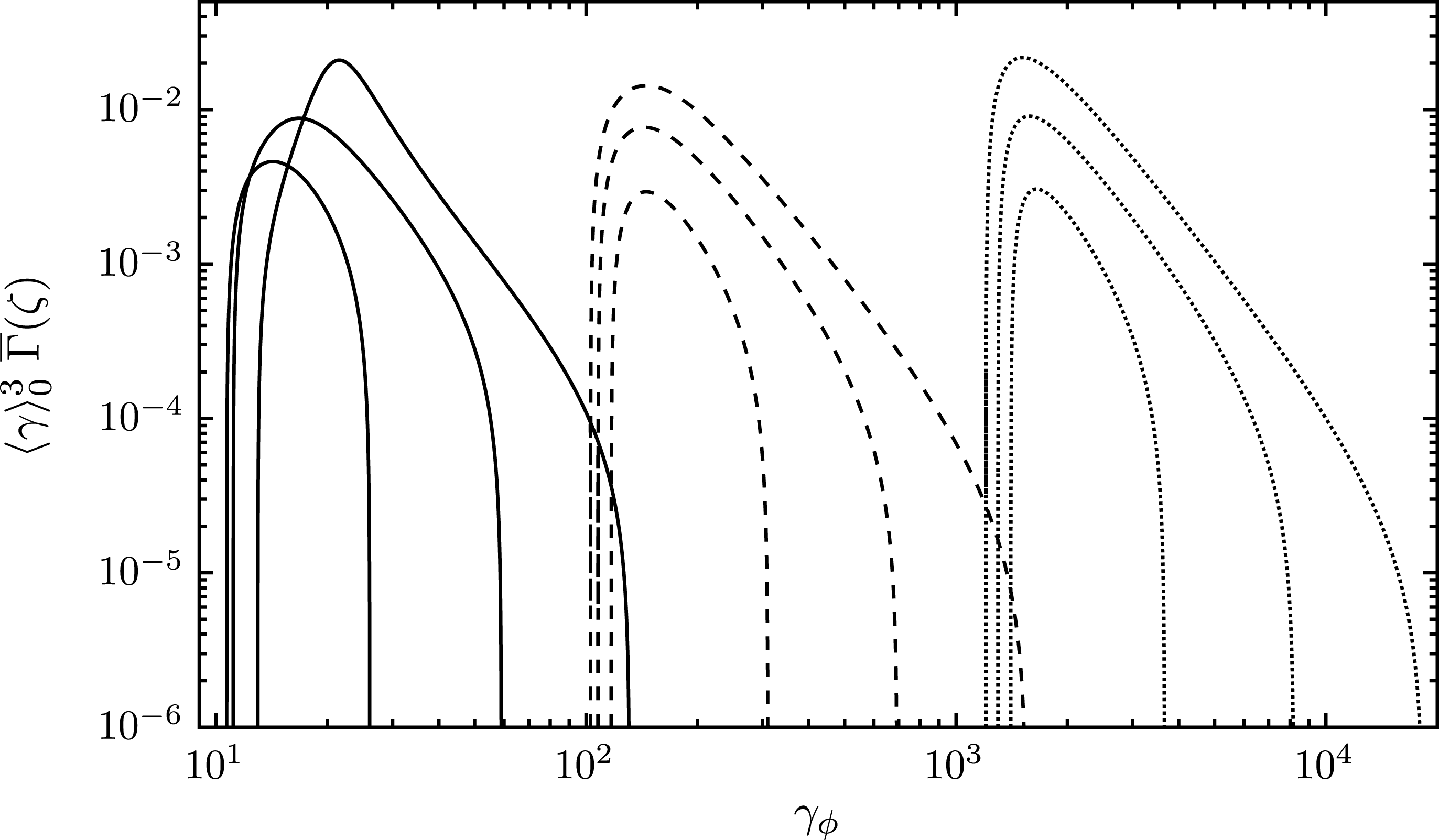
Plots of the absolute value of the negative region of the fractional absorption coefficient $\overline{\unicode[STIX]{x1D6E4}}_{L}(\unicode[STIX]{x1D701})$ , scaled by $\langle \unicode[STIX]{x1D6FE}\rangle _{0}^{3}$ , as a function of $\unicode[STIX]{x1D6FE}_{\unicode[STIX]{x1D719}}$ for $\unicode[STIX]{x1D70C}_{0}=1$ (solid), $\unicode[STIX]{x1D70C}_{0}=0.1$ (dashed) and $\unicode[STIX]{x1D70C}_{0}=0.01$ (dotted). For each $\unicode[STIX]{x1D70C}_{0}$ we use $\unicode[STIX]{x1D700}_{\unicode[STIX]{x1D70C}}=1$ , $\unicode[STIX]{x1D700}_{n}=10^{-3}$ and $\unicode[STIX]{x1D6FE}_{\text{b}}/\unicode[STIX]{x1D6FE}_{\text{b},\min }=2$ (bottom), 3.2 (middle) and 5 (top). The right footpoint of each curve corresponds to $\unicode[STIX]{x1D6FE}_{\unicode[STIX]{x1D719}}\approx \unicode[STIX]{x1D6FE}_{\text{b}}$ .

In figure 1 we show plots of the absolute value of the negative region of the fractional absorption coefficient $\overline{\unicode[STIX]{x1D6E4}}_{L}(\unicode[STIX]{x1D701})$ , scaled by $\langle \unicode[STIX]{x1D6FE}\rangle _{0}^{3}$ , as a function of $\unicode[STIX]{x1D6FE}_{\unicode[STIX]{x1D719}}$ for $\unicode[STIX]{x1D70C}_{0}=1$ (solid), $\unicode[STIX]{x1D70C}_{0}=0.1$ (dashed) and $\unicode[STIX]{x1D70C}_{0}=0.01$ (dotted). For all values of $\unicode[STIX]{x1D70C}_{0}$ we use $\unicode[STIX]{x1D700}_{\unicode[STIX]{x1D70C}}=1$ , $\unicode[STIX]{x1D700}_{n}=10^{-3}$ and $\unicode[STIX]{x1D6FE}_{\text{b}}/\unicode[STIX]{x1D6FE}_{\text{b},\min }=2$ (bottom), 3.2 (middle) and 5 (top). The right footpoint of each curve corresponds to $\unicode[STIX]{x1D6FE}_{\unicode[STIX]{x1D719}}\approx \unicode[STIX]{x1D6FE}_{1}\approx \unicode[STIX]{x1D6FE}_{\text{b}}$ and the left hand corresponds to $\unicode[STIX]{x1D6FE}_{\unicode[STIX]{x1D719}}\approx \unicode[STIX]{x1D6FE}_{2}$ as defined in (3.13). It is evident that the region over which $\overline{\unicode[STIX]{x1D6E4}}_{L}(\unicode[STIX]{x1D701})$ is negative widens as $\unicode[STIX]{x1D6FE}_{\text{b}}$ increases, however, the full width at half-maximum (FWHM) remains relatively unaffected. The maximum negative value of $\overline{\unicode[STIX]{x1D6E4}}_{L}(\unicode[STIX]{x1D701})$ occurs at $\unicode[STIX]{x1D6FE}_{\unicode[STIX]{x1D719}}\approx (12\pm 4)\langle \unicode[STIX]{x1D6FE}\rangle _{0}\sim \unicode[STIX]{x1D6FE}_{\text{b},\min }$ which is at higher phase velocity than the peak of $\unicode[STIX]{x1D701}^{2}\text{Re}\,W_{0}(\unicode[STIX]{x1D701})$ at $\unicode[STIX]{x1D701}=\unicode[STIX]{x1D701}_{\text{m0}}$ corresponding to $\unicode[STIX]{x1D6FE}_{\unicode[STIX]{x1D719}}\approx \unicode[STIX]{x1D6FE}_{\text{m0}}\approx 6.2\langle \unicode[STIX]{x1D6FE}\rangle _{0}$ , where $\unicode[STIX]{x1D6FE}_{\text{m0}}=\unicode[STIX]{x1D6FE}|_{\unicode[STIX]{x1D6FD}=\unicode[STIX]{x1D701}_{\text{m0}}}$ .

Figure 2.

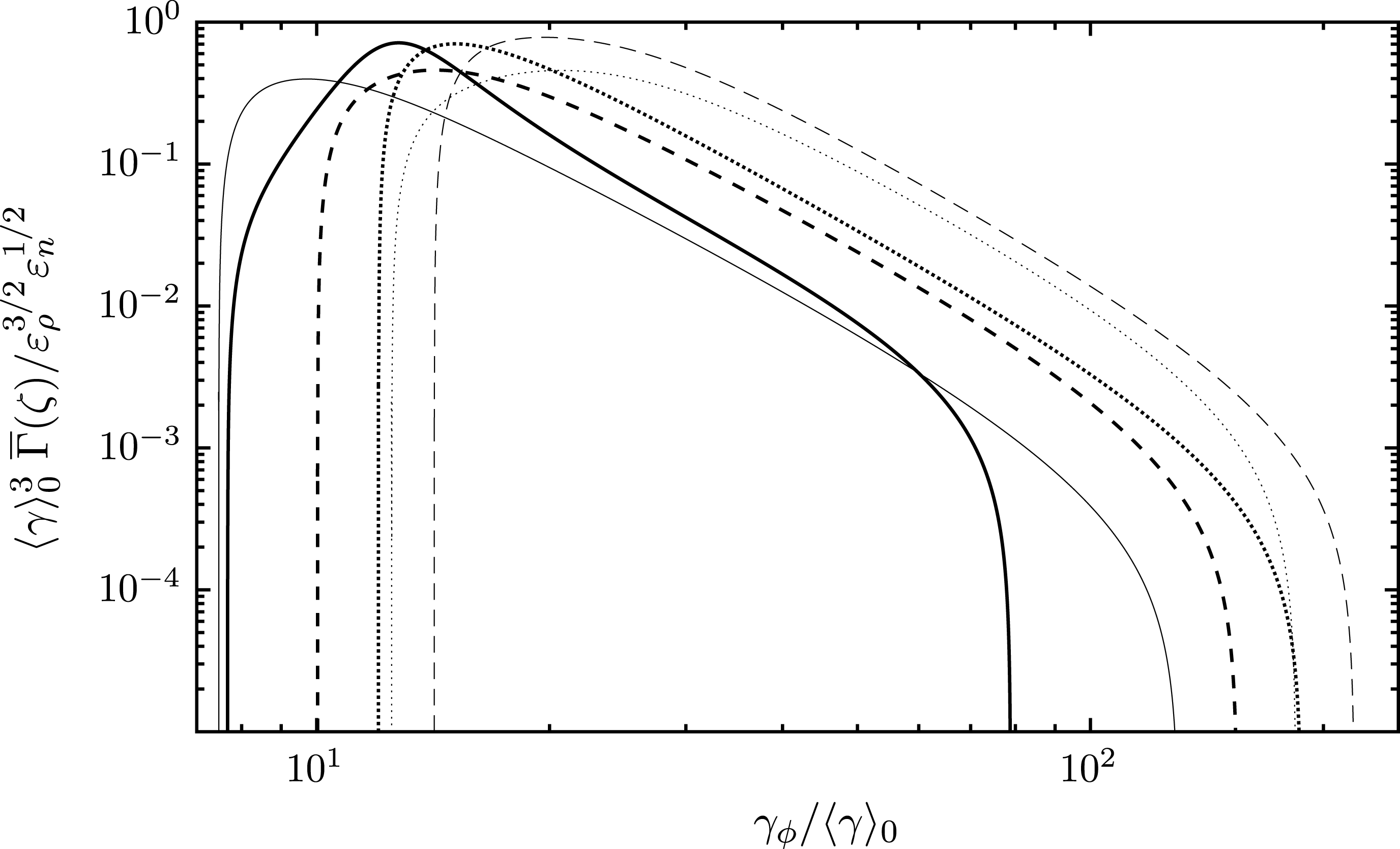
Plots of the absolute value of the negative region of $\overline{\unicode[STIX]{x1D6E4}}_{L}(\unicode[STIX]{x1D701})$ , scaled by $\langle \unicode[STIX]{x1D6FE}\rangle _{0}^{3}/\unicode[STIX]{x1D700}_{\unicode[STIX]{x1D70C}}^{3/2}\unicode[STIX]{x1D700}_{n}^{1/2}$ , as a function of $\unicode[STIX]{x1D6FE}_{\unicode[STIX]{x1D719}}$ , scaled by $1/\langle \unicode[STIX]{x1D6FE}\rangle _{0}$ , for $\unicode[STIX]{x1D6FE}_{\text{b}}/\unicode[STIX]{x1D6FE}_{\text{b},\min }=3.2$ and default values $(\unicode[STIX]{x1D70C}_{0},\unicode[STIX]{x1D700}_{\unicode[STIX]{x1D70C}},\unicode[STIX]{x1D700}_{n})=(0.1,1,10^{-3})$ . We vary $\unicode[STIX]{x1D70C}_{0}\rightarrow 1$ (solid), $\unicode[STIX]{x1D70C}_{0}\rightarrow 0.01$ (dotted), $\unicode[STIX]{x1D700}_{n}\rightarrow 10^{-4}$ (thin-dotted), $\unicode[STIX]{x1D700}_{n}\rightarrow 10^{-2}$ (thin-solid) and $\unicode[STIX]{x1D700}_{n}\rightarrow 0.1$ (thin-dashed).

In figure 2 we show plots of the absolute value of the negative region of $\overline{\unicode[STIX]{x1D6E4}}_{L}(\unicode[STIX]{x1D701})$ , scaled by $\langle \unicode[STIX]{x1D6FE}\rangle _{0}^{3}/\unicode[STIX]{x1D700}_{\unicode[STIX]{x1D70C}}^{3/2}\unicode[STIX]{x1D700}_{n}^{1/2}$ , as a function of $\unicode[STIX]{x1D6FE}_{\unicode[STIX]{x1D719}}$ , scaled by $1/\langle \unicode[STIX]{x1D6FE}\rangle _{0}$ , for $\unicode[STIX]{x1D6FE}_{\text{b}}/\unicode[STIX]{x1D6FE}_{\text{b},\min }=3.2$ and default values $(\unicode[STIX]{x1D70C}_{0},\unicode[STIX]{x1D700}_{\unicode[STIX]{x1D70C}},\unicode[STIX]{x1D700}_{n})=(0.1,1,10^{-3})$ . We vary $\unicode[STIX]{x1D70C}_{0}\rightarrow 1$ (solid), $\unicode[STIX]{x1D70C}_{0}\rightarrow 0.01$ (dotted), $\unicode[STIX]{x1D700}_{n}\rightarrow 10^{-4}$ (thin-dotted), $\unicode[STIX]{x1D700}_{n}\rightarrow 10^{-2}$ (thin-solid) and $\unicode[STIX]{x1D700}_{n}\rightarrow 0.1$ (thin-dashed). This shows that the location of the peak roughly scales with $1/\langle \unicode[STIX]{x1D6FE}\rangle _{0}$ and its height with $\langle \unicode[STIX]{x1D6FE}\rangle _{0}^{3}/\unicode[STIX]{x1D700}_{\unicode[STIX]{x1D70C}}^{3/2}\unicode[STIX]{x1D700}_{n}^{1/2}$ .

3.3 Penrose criterion

In appendix A we derive a necessary and sufficient condition for temporal kinetic plasma instability ( $\text{Im}\,\unicode[STIX]{x1D714}>0$ ): the solution $\unicode[STIX]{x1D714}^{2}=\unicode[STIX]{x1D714}_{\text{p}0}^{2}z^{2}W(z)$ to the dispersion equation $K_{33}(\unicode[STIX]{x1D714},k_{\Vert })=0$ corresponds to a growing mode provided that $\text{Re}\,z^{2}W(z)$ is positive when $\text{Im}\,z^{2}W(z)$ switches sign from negative to positive at $z=\unicode[STIX]{x1D701}_{2}$ , where $\unicode[STIX]{x1D701}_{2}$ corresponds to the phase at which $g(u)|_{\unicode[STIX]{x1D6FD}=\unicode[STIX]{x1D701}_{2}}$ is a minimum with $\text{d}g(u)/\text{d}\unicode[STIX]{x1D6FD}|_{\unicode[STIX]{x1D6FD}=\unicode[STIX]{x1D701}_{2}}=0$ . When the separation condition is satisfied, the Penrose criterion guarantees the existence of kinetic instability.

3.4 Bandwidth of growing waves

A restriction on the maser version of any instability is that the growth rate must be smaller than the bandwidth of the growing waves. This condition is required for the random phase approximation to be valid, with the bandwidth determining the rate of phase mixing of the growing waves. If the growth rate were to exceed the bandwidth of the growing waves, the initial phase would be remembered, and a phase-coherent wave would grow. The bandwidth of the growing waves provides a maximum value for the growth rate of the maser instability.

In estimating the bandwidth of the growing L mode waves in a pulsar plasma, it is not obvious how one can appeal to the analogy with the non-relativistic thermal case, or its relativistic generalization to a Gaussian distribution. This is because the dispersion relation $\unicode[STIX]{x1D714}=\unicode[STIX]{x1D714}_{L0}(\unicode[STIX]{x1D701})$ is a rapidly varying function of $\unicode[STIX]{x1D701}$ for the values of interest between the maximum of the RPDF $\unicode[STIX]{x1D701}^{2}\text{Re}\,W_{0}(\unicode[STIX]{x1D701})$ at $\unicode[STIX]{x1D701}=\unicode[STIX]{x1D701}_{\text{m0}}$ and the light line $\unicode[STIX]{x1D701}=1$ . This large rate of change of frequency with phase speed needs to be taken into account in estimating the bandwidth. A small range $\unicode[STIX]{x0394}\unicode[STIX]{x1D701}$ corresponds to a very small fractional bandwidth. The range $\unicode[STIX]{x0394}\unicode[STIX]{x1D701}$ over which the fractional absorption $\overline{\unicode[STIX]{x1D6E4}}_{L}(\unicode[STIX]{x1D701})$ is negative determines the bandwidth of the growing wave $\unicode[STIX]{x0394}\unicode[STIX]{x1D714}$ through $\unicode[STIX]{x0394}\unicode[STIX]{x1D714}=\unicode[STIX]{x0394}\unicode[STIX]{x1D701}\text{d}\unicode[STIX]{x1D714}_{L}(\unicode[STIX]{x1D701})/\text{d}\unicode[STIX]{x1D701}|_{\unicode[STIX]{x1D701}=\unicode[STIX]{x1D701}_{0}}+\mathit{O}((\unicode[STIX]{x0394}\unicode[STIX]{x1D701})^{2})$ for some central $\unicode[STIX]{x1D701}_{0}$ . We estimate $\unicode[STIX]{x0394}\unicode[STIX]{x1D701}$ by the FWHM of the negative region of the fractional absorption coefficient $\overline{\unicode[STIX]{x1D6E4}}_{L}(\unicode[STIX]{x1D701})$ with $\unicode[STIX]{x1D701}_{0}=\unicode[STIX]{x1D701}_{\text{ma}}$ corresponding to the phase at which the magnitude of the negative absorption coefficient is a maximum. The fractional bandwidth is then given by

(3.14) $$\begin{eqnarray}\overline{\unicode[STIX]{x0394}\unicode[STIX]{x1D714}}_{\text{bw}}=\left(\frac{\unicode[STIX]{x0394}\unicode[STIX]{x1D714}}{\unicode[STIX]{x1D714}_{L}(\unicode[STIX]{x1D701}_{\text{ma}})}\right)_{\text{bw}}\approx \left.\frac{\text{d}[\unicode[STIX]{x1D701}^{2}\text{Re}\,W(\unicode[STIX]{x1D701})]/\text{d}\unicode[STIX]{x1D701}}{2\unicode[STIX]{x1D701}^{2}\text{Re}\,W(\unicode[STIX]{x1D701})}\right|_{\unicode[STIX]{x1D701}=\unicode[STIX]{x1D701}_{\text{ma}}}\unicode[STIX]{x0394}\unicode[STIX]{x1D701}=\left[1-\frac{1}{2R_{L}(\unicode[STIX]{x1D701}_{\text{ma}})}\right]\unicode[STIX]{x0394}\unicode[STIX]{x1D701}.\end{eqnarray}$$

Figure 3.

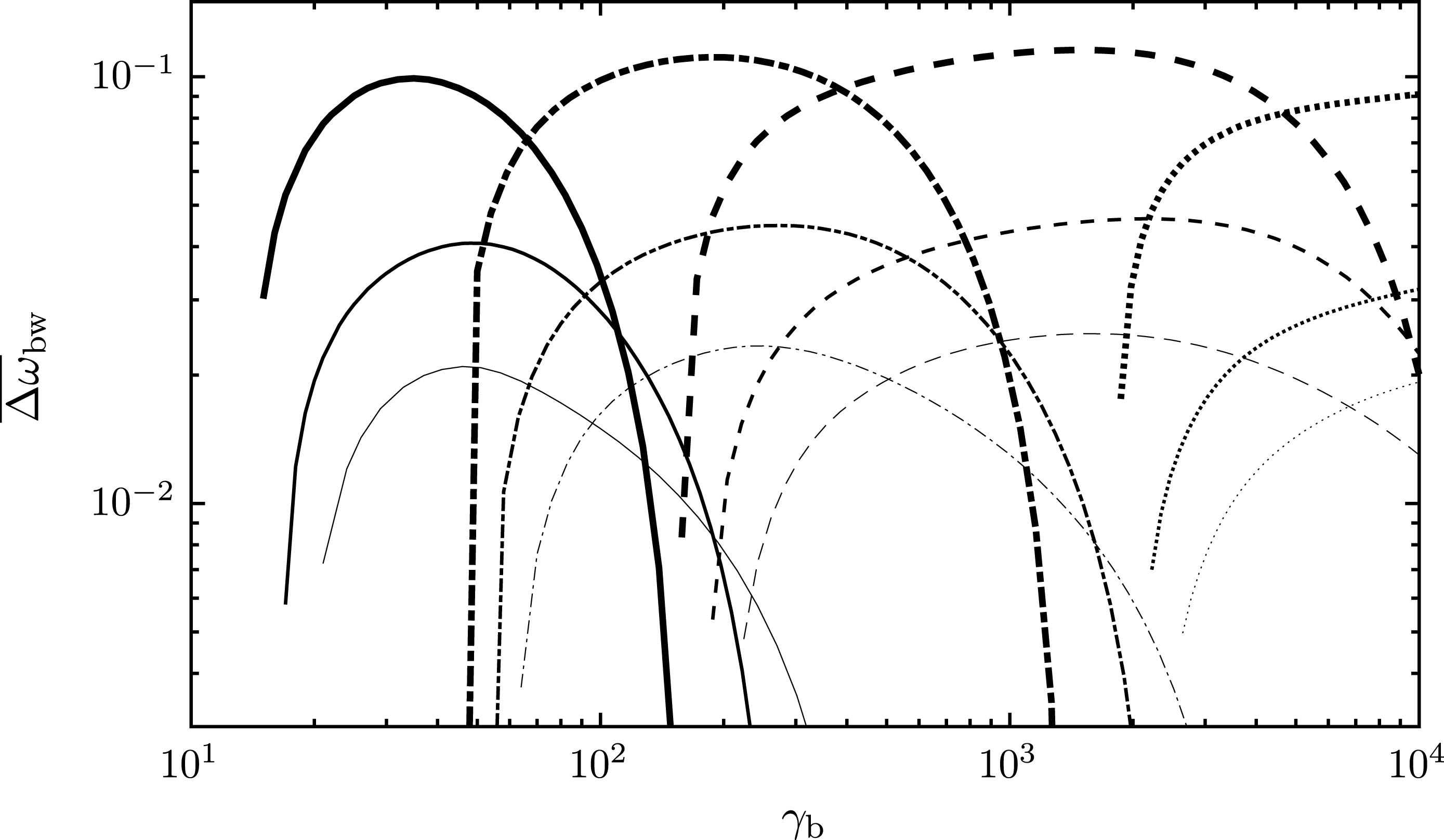
Plots of the fractional bandwidth $\overline{\unicode[STIX]{x0394}\unicode[STIX]{x1D714}}_{\text{bw}}$ over $\unicode[STIX]{x1D6FE}_{\text{b}}$ for $\unicode[STIX]{x1D70C}_{0}=1$ (solid), 0.32 (dash-dotted), 0.1 (dashed) and 0.01 (dotted). For each value of $\unicode[STIX]{x1D70C}_{0}$ we use $\unicode[STIX]{x1D700}_{\unicode[STIX]{x1D70C}}=1$ and $\unicode[STIX]{x1D700}_{n}=10^{-3}$ (thick), $10^{-4}$ (medium) and $10^{-5}$ (thin).

In figure 3 we show plots of the fractional bandwidth $\overline{\unicode[STIX]{x0394}\unicode[STIX]{x1D714}}_{\text{bw}}$ over $\unicode[STIX]{x1D6FE}_{\text{b}}$ for $\unicode[STIX]{x1D70C}_{0}=1$ (solid), 0.32 (dash-dotted), 0.1 (dashed) and 0.01 (dotted). For each value of $\unicode[STIX]{x1D70C}_{0}$ we use $\unicode[STIX]{x1D700}_{\unicode[STIX]{x1D70C}}=1$ and $\unicode[STIX]{x1D700}_{n}=10^{-3}$ (thick), $10^{-4}$ (medium) and $10^{-5}$ (thin). Using $\unicode[STIX]{x1D700}_{n}=10^{-3}$ , $10^{-4}$ , $10^{-5}$ , for $\unicode[STIX]{x1D70C}_{0}=1$ the fractional bandwidth is a maximum at $\unicode[STIX]{x1D6FE}_{\text{b}}\approx 35,49,46$ , for $\unicode[STIX]{x1D70C}=0.32$ the maxima are at $\unicode[STIX]{x1D6FE}_{\text{b}}\approx (1.9,2.8,2.4)\times 10^{2}$ , and for $\unicode[STIX]{x1D70C}_{0}=0.1$ the maxima are at $\unicode[STIX]{x1D6FE}_{\text{b}}\approx (1.6,2.1,1.6)\times 10^{3}$ , respectively. The maximum value of the fractional bandwidth is given by

(3.15) $$\begin{eqnarray}\overline{\unicode[STIX]{x0394}\unicode[STIX]{x1D714}}_{\text{bw},\max }\approx 2\times 10^{-3}\unicode[STIX]{x1D700}_{n}^{-1/3}.\end{eqnarray}$$

For the purpose of discussing the kinetic instability we are interested in the ratio of the growth rate to the bandwidth of the growing wave

(3.16) $$\begin{eqnarray}\unicode[STIX]{x1D700}_{L}=\frac{\overline{\unicode[STIX]{x1D6E4}}_{L}(\unicode[STIX]{x1D701}_{\text{ma}})}{\overline{\unicode[STIX]{x0394}\unicode[STIX]{x1D714}}_{\text{bw}}}.\end{eqnarray}$$

For maser growth through kinetic instability to be possible we require that the growth rate is smaller than the bandwidth of the growing wave so that phase mixing can occur. This is equivalent to requiring that $\unicode[STIX]{x1D700}_{L}<1$ .

Figure 4.

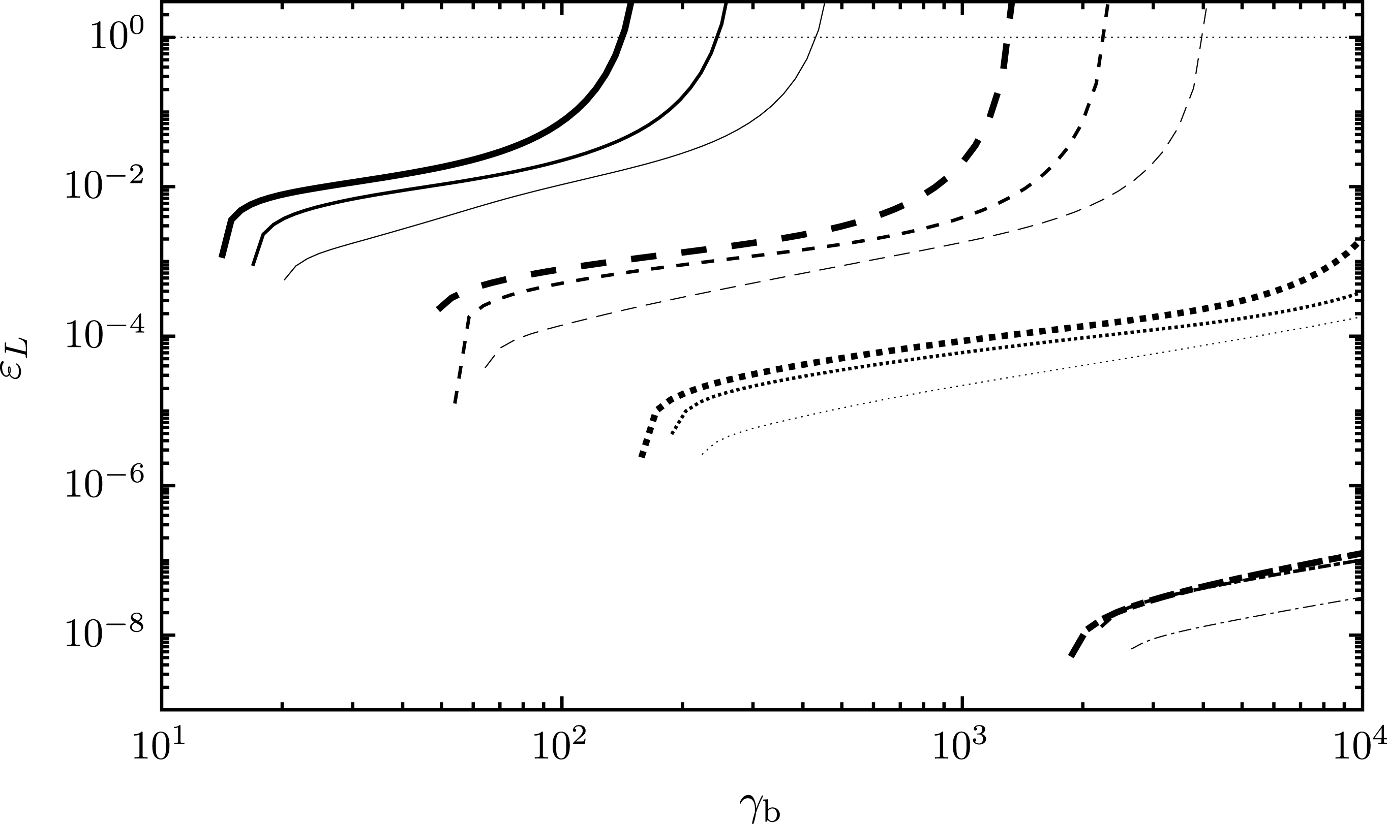
Plot $\unicode[STIX]{x1D700}_{L}$ over $\unicode[STIX]{x1D6FE}_{\text{b}}$ for $\unicode[STIX]{x1D70C}_{0}=1$ (solid), 0.32 (dashed), 0.1 (dotted) and 0.01 (dash-dotted). For each value of $\unicode[STIX]{x1D70C}_{0}$ we use $\unicode[STIX]{x1D700}_{\unicode[STIX]{x1D70C}}=1$ and $\unicode[STIX]{x1D700}_{n}=10^{-3}$ (thick), $10^{-4}$ (medium) and $10^{-5}$ (thin). The thin dotted horizontal line indicates the threshold $\unicode[STIX]{x1D700}_{L}=1$ .

In figure 4 we plot $\unicode[STIX]{x1D700}_{L}$ over $\unicode[STIX]{x1D6FE}_{\text{b}}$ for $\unicode[STIX]{x1D70C}_{0}=1$ (solid), 0.32 (dashed), 0.1 (dotted) and 0.01 (dash-dotted). For each value of $\unicode[STIX]{x1D70C}_{0}$ we use $\unicode[STIX]{x1D700}_{\unicode[STIX]{x1D70C}}=1$ and $\unicode[STIX]{x1D700}_{n}=10^{-3}$ (thick), $10^{-4}$ (medium) and $10^{-5}$ (thin). The thin dotted horizontal line indicates the threshold $\unicode[STIX]{x1D700}_{L}=1$ . For all values of $\unicode[STIX]{x1D70C}_{0}$ , each curve starts at $\unicode[STIX]{x1D6FE}_{\text{b}}\approx \unicode[STIX]{x1D6FE}_{\text{b},\min }$ . For $\unicode[STIX]{x1D70C}_{0}=1,0.32$ we have $\unicode[STIX]{x1D700}_{L}>1$ at $\unicode[STIX]{x1D6FE}_{\text{b}}\gtrsim (1.4,2.5,4.2)\times 10^{2}$ and $\unicode[STIX]{x1D6FE}_{\text{b}}\gtrsim (1.3,2.2,4)\times 10^{3}$ , respectively, for $\unicode[STIX]{x1D700}_{n}=(10^{-3},10^{-4},10^{-5})$ . The streaming Lorentz factor $\unicode[STIX]{x1D6FE}_{\text{b}}$ for which $\unicode[STIX]{x1D700}_{L}>1$ roughly scales as ${\sim}(25\text{-}23)/\unicode[STIX]{x1D700}_{n}^{1/4}\unicode[STIX]{x1D70C}_{0}^{2}$ for $\unicode[STIX]{x1D70C}_{0}=1-0.32$ . Furthermore, the curves corresponding to $\unicode[STIX]{x1D70C}_{0}=1$ , 0.32 do not extend to $\unicode[STIX]{x1D6FE}_{\text{b}}=10^{4}$ because growth is suppressed for $\unicode[STIX]{x1D6FE}_{\text{b}}\gtrsim (1.7,2.9,5)\times 10^{2}$ and $\unicode[STIX]{x1D6FE}_{\text{b}}\gtrsim (1.4,2.4,4.3)\times 10^{3}$ , respectively, for $\unicode[STIX]{x1D700}_{n}=(10^{-3},10^{-4},10^{-5})$ .

3.5 Comparison with the results of ELM

ELM considered wave growth in a pulsar plasma assuming a relativistically streaming Gaussian beam. These authors estimated both the growth rate and the bandwidth of the growing waves, and argued that the requirement that the bandwidth exceed the growth rate is so severe that it cannot be satisfied for plausible parameters in a pulsar plasma. Here we apply the same argument to a Lorentz-transformed Jüttner distribution.

For the relativistically streaming Gaussian distribution (2.8) the bandwidth of the growing waves was estimated by ELM to be $\unicode[STIX]{x0394}\unicode[STIX]{x1D714}_{\text{bw}}\approx |k_{\Vert }|c\unicode[STIX]{x0394}\unicode[STIX]{x1D6FD}$ , where $\unicode[STIX]{x0394}\unicode[STIX]{x1D6FD}\approx \unicode[STIX]{x1D6FD}\unicode[STIX]{x0394}\unicode[STIX]{x1D6FE}/\unicode[STIX]{x1D6FE}^{3}$ is the range of speeds over which the resonance applies. An analogy between a relativistically streaming Gaussian and a streaming Maxwellian allows this width to be identified as $\unicode[STIX]{x0394}\unicode[STIX]{x1D6FE}\rightarrow \unicode[STIX]{x1D6FE}_{\text{Tb}}$ around $\unicode[STIX]{x1D6FE}=\unicode[STIX]{x1D6FE}_{\text{b}}$ , giving $\unicode[STIX]{x0394}\unicode[STIX]{x1D714}_{\text{bw}}\approx |k_{\Vert }|c\unicode[STIX]{x1D6FE}_{\text{Tb}}/\unicode[STIX]{x1D6FE}_{\text{b}}^{3}$ . As in the non-relativistic case, the spread in phase speeds is identified as $\unicode[STIX]{x0394}\unicode[STIX]{x1D701}=\unicode[STIX]{x0394}\unicode[STIX]{x1D6FD}$ around the resonant value $\unicode[STIX]{x1D701}=\unicode[STIX]{x1D6FD}_{\text{b}}$ , corresponding to a spread $\unicode[STIX]{x0394}\unicode[STIX]{x1D6FE}_{\unicode[STIX]{x1D719}}$ about $\unicode[STIX]{x1D6FE}_{\unicode[STIX]{x1D719}}=\unicode[STIX]{x1D6FE}_{\text{b}}$ , with $\unicode[STIX]{x0394}\unicode[STIX]{x1D701}=\unicode[STIX]{x0394}\unicode[STIX]{x1D6FE}_{\unicode[STIX]{x1D719}}/\unicode[STIX]{x1D6FE}_{\unicode[STIX]{x1D719}}^{3}$ . ELM compared this bandwidth with the maximum growth rate for the kinetic instability due to the relativistically streaming Gaussian distribution, and found that the growth rate greatly exceeds the bandwidth for plausible parameters. We note that, although ELM took the dispersion relation for waves in pulsar plasma into account elsewhere, they did not take it into account explicitly in estimating this bandwidth.

ELM suggested that plausible parameters are $n_{1}/n_{0}\approx 10^{-3}$ which corresponds to $\unicode[STIX]{x1D700}_{n}=n_{1}/\unicode[STIX]{x1D6FE}_{\text{b}}n_{0}\approx 10^{-3}/\unicode[STIX]{x1D6FE}_{\text{b}}$ . The minimum separation streaming Lorentz factors required for $\unicode[STIX]{x1D70C}_{0}=1,0.1,0.01$ are $\unicode[STIX]{x1D6FE}_{\text{b},\min }\sim 10,10^{2},10^{3}$ , respectively, which implies corresponding $\unicode[STIX]{x1D700}_{n}$ of ${\sim}10^{-4}$ , $10^{-5}$ , $10^{-6}$ . The results of Arendt & Eilek (Reference Arendt and Eilek2002) suggest that particle distributions (background or beam) stream with Lorentz factors ${\sim}10^{2}{-}10^{3}$ in the pulsar frame. If one assumes that, in the pulsar frame, the rest frame of the background distribution streams with $\unicode[STIX]{x1D6FE}_{\text{s}}\sim 10^{2}{-}10^{3}$ then the rest frame of the beam must stream with Lorentz factor $\unicode[STIX]{x1D6FE}_{\text{r}}\sim 10^{3}{-}10^{4}$ for $\unicode[STIX]{x1D70C}_{0}=1$ ; $\unicode[STIX]{x1D6FE}_{\text{r}}\sim 10^{4}{-}10^{5}$ for $\unicode[STIX]{x1D70C}_{0}=0.1$ ; and $\unicode[STIX]{x1D6FE}_{\text{r}}\sim 10^{5}{-}10^{6}$ for $\unicode[STIX]{x1D70C}_{0}=0.01$ . The peak of negative absorption is at $\unicode[STIX]{x1D6FE}_{\unicode[STIX]{x1D719}}\sim 10\langle \unicode[STIX]{x1D6FE}\rangle _{0}$ which implies that for maximum wave growth we want $\unicode[STIX]{x1D6FE}_{\text{b}}\sim 10\langle \unicode[STIX]{x1D6FE}\rangle _{0}$ ; this roughly corresponds to $\unicode[STIX]{x1D6FE}_{\text{b},\min }$ . We may then write, for maximum fractional growth rate, $\unicode[STIX]{x1D6FE}_{\text{r}}\sim (10^{3}{-}10^{4})\langle \unicode[STIX]{x1D6FE}\rangle _{0}$ using $\unicode[STIX]{x1D6FE}_{\text{r}}=\unicode[STIX]{x1D6FE}_{\text{s}}\unicode[STIX]{x1D6FE}_{\text{b}}$ .

The maximum fractional growth rate may be approximated from figure 2 as

(3.17) $$\begin{eqnarray}|\overline{\unicode[STIX]{x1D6E4}}_{L}(\unicode[STIX]{x1D701})|_{\max }\sim \frac{\unicode[STIX]{x1D700}_{n}^{1/2}\unicode[STIX]{x1D700}_{\unicode[STIX]{x1D70C}}^{3/2}}{2\langle \unicode[STIX]{x1D6FE}\rangle _{0}^{3}}.\end{eqnarray}$$

For $\unicode[STIX]{x1D700}_{\unicode[STIX]{x1D70C}}=1$ , $\unicode[STIX]{x1D70C}_{0}=1,0.1,0.01$ and corresponding $\unicode[STIX]{x1D700}_{n}=10^{-4},10^{-5},10^{-6}$ we have, respectively,

(3.18) $$\begin{eqnarray}|\overline{\unicode[STIX]{x1D6E4}}_{L}(\unicode[STIX]{x1D701})|_{\max }\sim 10^{-3},10^{-6},10^{-11}.\end{eqnarray}$$

We conclude that wave growth through kinetic (or maser) instability is possible (in principle). This is different from the conclusion of ELM; this difference reflects the difference between the relativistically streaming Gaussian distribution that they assumed and the (much broader) Lorentz-transformed distribution that we assume, and for which the bandwidth is larger and the growth rate is smaller.

4.1 Reduction of the dispersion equation

In treating a reactive instability, one neglects the dissipative part of the response function, which plays a central role in the treatment of a kinetic instability. This corresponds to neglecting the dissipative part of the RPDF and the imaginary parts of $\unicode[STIX]{x1D714}$ and $k_{\Vert }$ , so that the response function (2.17) reduces to

(4.1) $$\begin{eqnarray}K_{33}(\unicode[STIX]{x1D714},k_{\Vert })=1-\unicode[STIX]{x1D714}_{\text{p}0}^{2}\frac{\unicode[STIX]{x1D701}^{2}\text{Re}\,W_{0}(\unicode[STIX]{x1D701})}{\unicode[STIX]{x1D714}^{2}}-\unicode[STIX]{x1D700}_{n}\unicode[STIX]{x1D714}_{\text{p0}}^{2}\frac{\unicode[STIX]{x1D701}^{\prime \prime 2}\text{Re}\,W_{1}^{\prime \prime }(\unicode[STIX]{x1D701}^{\prime \prime })}{\unicode[STIX]{x1D6FE}_{\text{b}}^{2}(\unicode[STIX]{x1D714}-\unicode[STIX]{x1D6FD}_{\text{b}}ck_{\Vert })^{2}}.\end{eqnarray}$$

In treating reactive instability we assume $k_{\Vert }=\text{Re}\,k_{\Vert }$ and comment on the spatial growth in the next section. To identify a reactive instability one needs to approximate the dispersion equation $K_{33}(\unicode[STIX]{x1D714},k_{\Vert })=0$ , implied by setting (4.1) to zero, by a polynomial in $\unicode[STIX]{x1D714}$ with real coefficients. The complex solutions then must appear in complex conjugate pairs, one of which describes an intrinsically growing wave.

The simplest cases of reactive instabilities are derived assuming a cold-plasma model, such that the spread in particle energies is neglected. For a cold background, $\unicode[STIX]{x1D70C}_{0}=\infty$ , and cold beam, $\unicode[STIX]{x1D70C}_{1}=\infty$ , one has $\unicode[STIX]{x1D701}^{2}\text{Re}\,W_{0}(\unicode[STIX]{x1D701})\rightarrow 1$ and $\unicode[STIX]{x1D701}^{\prime \prime 2}\text{Re}\,W_{1}^{\prime \prime }(\unicode[STIX]{x1D701}^{\prime \prime })\rightarrow 1$ so that (4.1) reproduces the well-known cold-plasma form for the dispersion equation for a relativistic cold weak-beam system,

(4.2) $$\begin{eqnarray}1-\frac{\unicode[STIX]{x1D714}_{\text{p}0}^{2}}{\unicode[STIX]{x1D714}^{2}}-\frac{\unicode[STIX]{x1D714}_{\text{p1}}^{2}}{\unicode[STIX]{x1D6FE}_{\text{b}}^{3}(\unicode[STIX]{x1D714}-\unicode[STIX]{x1D6FD}_{\text{b}}ck_{\Vert })^{2}}=0,\end{eqnarray}$$

which is a quartic equation in $\unicode[STIX]{x1D714}$ . A complication in reducing (4.1) to this form is that $\unicode[STIX]{x1D701}$ and $\unicode[STIX]{x1D701}^{\prime \prime }$ are implicit functions of $\unicode[STIX]{x1D714}$ . To proceed analytically, we ignore this complication, assuming that $\unicode[STIX]{x1D701}$ and $\unicode[STIX]{x1D701}^{\prime \prime }$ are constants. In our numerical results we solve (4.1) directly without additional assumptions.

A justification for assuming that $\unicode[STIX]{x1D701}$ and $\unicode[STIX]{x1D701}^{\prime \prime }$ are constants is that they are both close to unity, suggesting that one may approximate them by unity, giving

(4.3) $$\begin{eqnarray}\left.\begin{array}{@{}c@{}}\unicode[STIX]{x1D701}^{2}\text{Re}\,W_{0}(\unicode[STIX]{x1D701})\rightarrow \text{Re}\,W_{0}(1)=2\langle \unicode[STIX]{x1D6FE}\rangle _{0}-\langle 1/\unicode[STIX]{x1D6FE}\rangle _{0},\\ \unicode[STIX]{x1D701}^{\prime \prime 2}\text{Re}\,W_{1}^{\prime \prime }(\unicode[STIX]{x1D701}^{\prime \prime })\rightarrow \text{Re}\,W_{1}^{\prime \prime }(1)=2\langle \unicode[STIX]{x1D6FE}^{\prime \prime }\rangle _{1}^{\prime \prime }-\langle 1/\unicode[STIX]{x1D6FE}^{\prime \prime }\rangle _{1}^{\prime \prime },\end{array}\right\}\end{eqnarray}$$

where the right-hand expressions were derived in Part 1. For $\{\unicode[STIX]{x1D70C}_{0},\unicode[STIX]{x1D70C}_{1}\}\ll 1$ we may write $\text{Re}\,W_{0}(1)\approx 2\langle \unicode[STIX]{x1D6FE}\rangle _{0}$ and $\text{Re}\,W_{1}^{\prime \prime }(1)=2\langle \unicode[STIX]{x1D6FE}^{\prime \prime }\rangle _{1}^{\prime \prime }$ . With the implicit dependence on $\unicode[STIX]{x1D714}$ through $\unicode[STIX]{x1D701}$ and $\unicode[STIX]{x1D701}^{\prime \prime }$ neglected in this way, the dispersion equation (4.1) becomes cold-plasma like and has the form

(4.4) $$\begin{eqnarray}K_{33}(\unicode[STIX]{x1D714},k_{\Vert })=1-\frac{\unicode[STIX]{x1D714}_{L0}^{2}(1)}{\unicode[STIX]{x1D714}^{2}}-\frac{\unicode[STIX]{x1D714}_{L1}^{\prime \prime 2}(1)}{\unicode[STIX]{x1D6FE}_{\text{b}}^{2}(\unicode[STIX]{x1D714}-\unicode[STIX]{x1D6FD}_{\text{b}}ck_{\Vert })^{2}},\end{eqnarray}$$

where $\unicode[STIX]{x1D714}_{L0}^{2}(\unicode[STIX]{x1D701})=\unicode[STIX]{x1D714}_{\text{p}0}^{2}\unicode[STIX]{x1D701}^{2}\text{Re}\,W_{0}(\unicode[STIX]{x1D701})$ and $\unicode[STIX]{x1D714}_{L1}^{\prime \prime 2}(\unicode[STIX]{x1D701}^{\prime \prime })=\unicode[STIX]{x1D700}_{n}\unicode[STIX]{x1D714}_{\text{p}0}^{2}\unicode[STIX]{x1D701}^{\prime \prime 2}\text{Re}\,W_{1}^{\prime \prime }(\unicode[STIX]{x1D701}^{\prime \prime })$ . With these assumptions, dispersion equation (4.4) becomes a polynomial of degree four in $\unicode[STIX]{x1D714}$ with real coefficients.

Figure 5.

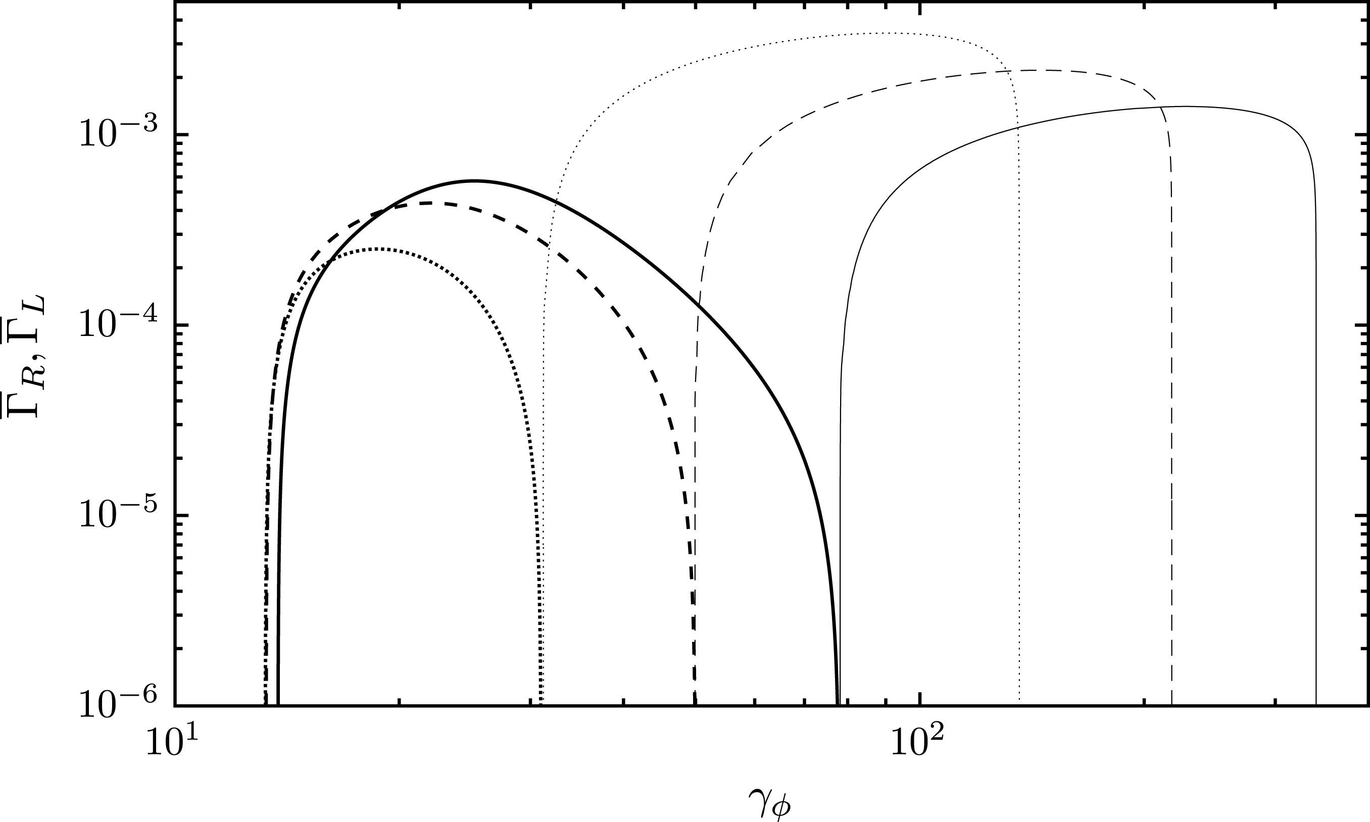
Plots of the fractional growth rate for reactive instability $\overline{\unicode[STIX]{x1D6E4}}_{R}$ (thin curves) and for kinetic instability $\overline{\unicode[STIX]{x1D6E4}}_{L}$ (thick curves) for $\unicode[STIX]{x1D70C}_{0}=1$ , $\unicode[STIX]{x1D700}_{\unicode[STIX]{x1D70C}}=1$ , $\unicode[STIX]{x1D700}_{n}=10^{-4}$ , and $\unicode[STIX]{x1D6FE}_{\text{b}}/\unicode[STIX]{x1D6FE}_{\text{b},\min }=2$ (dotted), 3.2 (dashed) and 5 (solid).

4.1.1 Numerical solutions of the dispersion equation

We numerically solve (4.1), treating $\unicode[STIX]{x1D701}$ as a function of $\unicode[STIX]{x1D714}_{r}$ , for $\unicode[STIX]{x1D714}=\unicode[STIX]{x1D714}_{r}+\text{i}\unicode[STIX]{x1D714}_{i}$ and define the fractional growth rate of (temporal) reactive instability as

(4.5) $$\begin{eqnarray}\overline{\unicode[STIX]{x1D6E4}}_{R}=2\frac{\unicode[STIX]{x1D714}_{i}}{\unicode[STIX]{x1D714}_{r}}.\end{eqnarray}$$

Figure 5 shows plots of the fractional growth rate for reactive instability $\overline{\unicode[STIX]{x1D6E4}}_{R}$ (thin curves) and for kinetic instability $\overline{\unicode[STIX]{x1D6E4}}_{L}$ (thick curves) for $\unicode[STIX]{x1D70C}_{0}=1$ , $\unicode[STIX]{x1D700}_{\unicode[STIX]{x1D70C}}=1$ , $\unicode[STIX]{x1D700}_{n}=10^{-4}$ and  $\unicode[STIX]{x1D6FE}_{\text{b}}/\unicode[STIX]{x1D6FE}_{\text{b},\min }=2$ (dotted), 3.2 (dashed) and 5 (solid). It is clear that reactive instability and kinetic instability apply over different ranges of phase velocity $\unicode[STIX]{x1D701}$ ; however, they overlap when plotted over wavenumber $k_{\Vert }$ which will become apparent below. Reactive instability grows faster, and applies over a wider phase velocity range and closer to the light line $\unicode[STIX]{x1D701}=1$ than kinetic instability.

Reactive instability applies over $\unicode[STIX]{x1D6FE}_{\text{b}}\lesssim \unicode[STIX]{x1D6FE}_{\unicode[STIX]{x1D719}}\lesssim \unicode[STIX]{x1D6FE}|_{\unicode[STIX]{x1D6FD}=\unicode[STIX]{x1D701}_{01}}$ where $\unicode[STIX]{x1D701}_{01}$ is where $\unicode[STIX]{x1D701}^{2}\text{Re}\,W_{1}(\unicode[STIX]{x1D701})$ is zero. In the rest frame of the beam $\unicode[STIX]{x1D701}_{01}^{\prime \prime }\approx 1-\unicode[STIX]{x1D6FC}_{1}\unicode[STIX]{x1D70C}_{1}$ with $\unicode[STIX]{x1D6FC}_{1}\approx 0.1$ for $\unicode[STIX]{x1D70C}_{1}=1$ and $\unicode[STIX]{x1D6FC}_{1}\approx 0.144$ for $\unicode[STIX]{x1D70C}_{1}\ll 1$ (Part 1). This corresponds to $\unicode[STIX]{x1D6FE}|_{\unicode[STIX]{x1D6FD}=\unicode[STIX]{x1D701}_{01}}\approx 4.4\unicode[STIX]{x1D6FE}_{\text{b}}$ for $\unicode[STIX]{x1D70C}_{1}=1$ and $\unicode[STIX]{x1D6FE}|_{\unicode[STIX]{x1D6FD}=\unicode[STIX]{x1D701}_{01}}\approx 3.5\unicode[STIX]{x1D6FE}_{\text{b}}\langle \unicode[STIX]{x1D6FE}\rangle _{0}/\unicode[STIX]{x1D700}_{\unicode[STIX]{x1D70C}}$ for $\unicode[STIX]{x1D70C}_{1}\ll 1$ .

4.2 Resonant reactive instability

The most familiar form of a reactive weak-beam instability is the solution of a cubic equation. To derive this case, we treat the contribution of the beam as a perturbation to that of the background so that to zeroth order the frequency is given by $\unicode[STIX]{x1D714}_{L0}(1)$ . It is convenient to assume $k_{\Vert }=\text{Re}\,k_{\Vert }$ and introduce

(4.6a,b ) $$\begin{eqnarray}\unicode[STIX]{x1D6FF}\unicode[STIX]{x1D714}=\unicode[STIX]{x1D714}-\unicode[STIX]{x1D714}_{L0}(1),\quad \unicode[STIX]{x1D6FF}\unicode[STIX]{x1D714}_{0}=\unicode[STIX]{x1D714}_{L0}(1)-k_{\Vert }c\unicode[STIX]{x1D6FD}_{\text{b}},\end{eqnarray}$$

with $|\unicode[STIX]{x1D6FF}\unicode[STIX]{x1D714}/\unicode[STIX]{x1D714}_{L0}(1)|\ll 1$ so that $K_{33}(\unicode[STIX]{x1D714},k_{\Vert })=0$ in (4.4) may be approximated as

(4.7) $$\begin{eqnarray}\overline{\unicode[STIX]{x1D6FF}\unicode[STIX]{x1D714}}(\overline{\unicode[STIX]{x1D6FF}\unicode[STIX]{x1D714}}+\overline{\unicode[STIX]{x1D6FF}\unicode[STIX]{x1D714}}_{0})^{2}\approx 1,\end{eqnarray}$$

with

(4.8) $$\begin{eqnarray}\frac{\unicode[STIX]{x1D6FF}\unicode[STIX]{x1D714}}{\overline{\unicode[STIX]{x1D6FF}\unicode[STIX]{x1D714}}}=\frac{\unicode[STIX]{x1D6FF}\unicode[STIX]{x1D714}_{0}}{\overline{\unicode[STIX]{x1D6FF}\unicode[STIX]{x1D714}}_{0}}=[\unicode[STIX]{x1D714}_{L0}(1)\unicode[STIX]{x1D714}_{L1}^{\prime \prime 2}(1)/2\unicode[STIX]{x1D6FE}_{\text{b}}^{2}]^{1/3}.\end{eqnarray}$$

The maximum growth rate is obtained when $|\unicode[STIX]{x1D6FF}\unicode[STIX]{x1D714}_{0}|\ll |\unicode[STIX]{x1D6FF}\unicode[STIX]{x1D714}|$ so that (4.7) reduces to $(\overline{\unicode[STIX]{x1D6FF}\unicode[STIX]{x1D714}})^{3}\approx 1$ with solutions

(4.9a,b ) $$\begin{eqnarray}\overline{\unicode[STIX]{x1D6FF}\unicode[STIX]{x1D714}}=1,\quad \overline{\unicode[STIX]{x1D6FF}\unicode[STIX]{x1D714}}=-(1\pm i\sqrt{3})/2.\end{eqnarray}$$

The growing solution, referred to as the resonant reactive instability, is

(4.10) $$\begin{eqnarray}\unicode[STIX]{x1D714}=\unicode[STIX]{x1D714}_{L0}(\unicode[STIX]{x1D701})\left[1-(1-i\sqrt{3})\left(\frac{\unicode[STIX]{x1D714}_{L1}^{\prime \prime 2}(1)}{16\unicode[STIX]{x1D6FE}_{\text{b}}^{2}\unicode[STIX]{x1D714}_{L0}^{2}(1)}\right)^{1/3}\right].\end{eqnarray}$$

The fractional growth rate of the resonant reactive instability is then given by

(4.11) $$\begin{eqnarray}\overline{\unicode[STIX]{x1D6E4}}_{\text{rr}}=2\frac{\unicode[STIX]{x1D714}_{i}}{\unicode[STIX]{x1D714}_{r}}\approx \sqrt{3}\left(\frac{\unicode[STIX]{x1D700}_{n}\langle \unicode[STIX]{x1D6FE}^{\prime \prime }\rangle _{1}^{\prime \prime }}{2\unicode[STIX]{x1D6FE}_{\text{b}}^{2}\langle \unicode[STIX]{x1D6FE}\rangle _{0}}\right)^{1/3}=\frac{\sqrt{3}}{\unicode[STIX]{x1D6FE}_{\text{b}}}\left(\frac{n_{1}\langle \unicode[STIX]{x1D6FE}^{\prime \prime }\rangle _{1}^{\prime \prime }}{2n_{0}\langle \unicode[STIX]{x1D6FE}\rangle _{0}}\right)^{1/3},\end{eqnarray}$$

where we use $\unicode[STIX]{x1D714}_{L0}^{2}(1)\approx 2\unicode[STIX]{x1D714}_{\text{p}0}^{2}\langle \unicode[STIX]{x1D6FE}\rangle _{0}$ , $\unicode[STIX]{x1D714}_{L1}^{\prime \prime 2}(1)\approx 2\unicode[STIX]{x1D700}_{n}\unicode[STIX]{x1D714}_{\text{p}0}^{2}\langle \unicode[STIX]{x1D6FE}^{\prime \prime }\rangle _{1}^{\prime \prime }$ and assume $\unicode[STIX]{x1D700}_{n}\langle \unicode[STIX]{x1D6FE}^{\prime \prime }\rangle _{1}^{\prime \prime }/2\unicode[STIX]{x1D6FE}_{\text{b}}^{2}\langle \unicode[STIX]{x1D6FE}\rangle _{0}$ $\ll 1$ . The fractional growth rate of the resonant reactive instability decreases with increasing streaming Lorentz factor $\unicode[STIX]{x1D6FE}_{\text{b}}$ and increases with $\unicode[STIX]{x1D700}_{n}$ . The fractional growth rate does not depend independently on the temperatures of the two distributions, described by the mean Lorentz factors, $\langle \unicode[STIX]{x1D6FE}\rangle _{0}$ and $\langle \unicode[STIX]{x1D6FE}^{\prime \prime }\rangle _{1}^{\prime \prime }$ , but only on the ratio of these quantities. This lack of dependence on temperature is not surprising as we effectively approximate the background and the beam as cold distributions through ignoring the implicit dependence of $\unicode[STIX]{x1D701}$ and $\unicode[STIX]{x1D701}^{\prime \prime }$ on $\unicode[STIX]{x1D714}$ .

The analytical approximation (4.11) is supported by numerical solutions of (4.1) where $\unicode[STIX]{x1D701}$ and $\unicode[STIX]{x1D701}^{\prime \prime }$ are treated as functions of $\unicode[STIX]{x1D714}$ . The thin-dotted curve in figure 5 corresponds to $\unicode[STIX]{x1D70C}_{0}=1$ , $\unicode[STIX]{x1D700}_{\unicode[STIX]{x1D70C}}=1$ , $\unicode[STIX]{x1D700}_{n}=10^{-4}$ and $\unicode[STIX]{x1D6FE}_{\text{b}}\approx 32$ with peak value $\overline{\unicode[STIX]{x1D6E4}}_{R}\approx 3.4\times 10^{-3}$ . For these parameter values we obtain $\overline{\unicode[STIX]{x1D6E4}}_{\text{rr}}\approx 6.3\times 10^{-3}$ using (4.11).

4.3 Non-resonant reactive instability

In (4.4), the contribution of the third term is significant when $\unicode[STIX]{x1D714}-\unicode[STIX]{x1D6FD}_{\text{b}}ck_{\Vert }$ is small since $\unicode[STIX]{x1D700}_{n}\ll 1$ . Introducing

(4.12) $$\begin{eqnarray}\unicode[STIX]{x1D6FF}\unicode[STIX]{x1D714}_{1}=\unicode[STIX]{x1D714}-\unicode[STIX]{x1D6FD}_{\text{b}}ck_{\Vert },\end{eqnarray}$$

with $|\unicode[STIX]{x1D6FF}\unicode[STIX]{x1D714}_{1}/\unicode[STIX]{x1D6FD}_{\text{b}}ck_{\Vert }|\ll 1$ allows us to write (4.4) as

(4.13) $$\begin{eqnarray}K_{33}(\unicode[STIX]{x1D714},k_{\Vert })\approx 1-\frac{\unicode[STIX]{x1D714}_{L0}^{2}(1)}{(\unicode[STIX]{x1D6FD}_{\text{b}}ck_{\Vert })^{2}}-\frac{\unicode[STIX]{x1D714}_{L1}^{\prime \prime 2}(1)}{\unicode[STIX]{x1D6FE}_{\text{b}}^{2}(\unicode[STIX]{x1D6FF}\unicode[STIX]{x1D714}_{1})^{2}},\end{eqnarray}$$

with $K_{33}(\unicode[STIX]{x1D714},k_{\Vert })=0$ having solutions

(4.14) $$\begin{eqnarray}\unicode[STIX]{x1D714}=\unicode[STIX]{x1D6FD}_{\text{b}}ck_{\Vert }\pm \frac{\unicode[STIX]{x1D6FD}_{\text{b}}ck_{\Vert }\unicode[STIX]{x1D714}_{L1}^{\prime \prime }(1)/\unicode[STIX]{x1D6FE}_{\text{b}}}{[(\unicode[STIX]{x1D6FD}_{\text{b}}ck_{\Vert })^{2}-\unicode[STIX]{x1D714}_{L0}^{2}(1)]^{1/2}}.\end{eqnarray}$$

A growing mode ( $\unicode[STIX]{x1D714}_{i}>0$ ) exists only if $\unicode[STIX]{x1D6FD}_{\text{b}}ck_{\Vert }<\unicode[STIX]{x1D714}_{L0}(1)$ . This condition agrees with our discussion that reactive instability applies over $\unicode[STIX]{x1D6FE}_{\text{b}}\lesssim \unicode[STIX]{x1D6FE}_{\unicode[STIX]{x1D719}}\lesssim \unicode[STIX]{x1D6FE}|_{\unicode[STIX]{x1D6FD}=\unicode[STIX]{x1D701}_{01}}$ (see also figure 6 below). This is the non-resonant unstable beam mode (Gedalin, Gruman & Melrose Reference Gedalin, Gruman and Melrose2002a ) with real frequency $\unicode[STIX]{x1D714}_{r}\approx \unicode[STIX]{x1D6FD}_{\text{b}}ck_{\Vert }$ . The non-resonant fractional absorption coefficient is given by

(4.15) $$\begin{eqnarray}\overline{\unicode[STIX]{x1D6E4}}_{\text{nr}}=2\frac{\unicode[STIX]{x1D714}_{i}}{\unicode[STIX]{x1D714}_{r}}=\frac{2\unicode[STIX]{x1D714}_{L1}^{\prime \prime }(1)/\unicode[STIX]{x1D6FE}_{\text{b}}}{[\unicode[STIX]{x1D714}_{L0}^{2}(1)-(\unicode[STIX]{x1D6FD}_{\text{b}}ck_{\Vert })^{2}]^{1/2}}\approx \left(\frac{2}{\unicode[STIX]{x1D6FE}_{\text{b}}}\right)^{3/2}\left(\frac{n_{1}\langle \unicode[STIX]{x1D6FE}^{\prime \prime }\rangle _{1}^{\prime \prime }}{2n_{0}\langle \unicode[STIX]{x1D6FE}\rangle _{0}}\right)^{1/2}\left[1-\frac{(\unicode[STIX]{x1D6FD}_{\text{b}}ck_{\Vert })^{2}}{2\langle \unicode[STIX]{x1D6FE}\rangle _{0}\unicode[STIX]{x1D714}_{\text{p}0}^{2}}\right]^{-1/2}.\end{eqnarray}$$

Clearly (4.14) and (4.15) break down as $\unicode[STIX]{x1D6FD}_{\text{b}}ck_{\Vert }\rightarrow \unicode[STIX]{x1D714}_{L0}(1)$ . This limit corresponds to the resonant case as treated above where $\unicode[STIX]{x1D714}_{r}\approx \unicode[STIX]{x1D714}_{L0}(1)$ instead of $\unicode[STIX]{x1D714}_{r}\approx \unicode[STIX]{x1D6FD}_{\text{b}}ck_{\Vert }$ in the non-resonant case. We may approximate the ratio of the resonant to non-resonant fractional growth rate as

(4.16) $$\begin{eqnarray}\frac{\overline{\unicode[STIX]{x1D6E4}}_{\text{rr}}}{\overline{\unicode[STIX]{x1D6E4}}_{\text{nr}}}\approx \sqrt{3}\left(\frac{\unicode[STIX]{x1D6FE}_{\text{b}}}{8}\right)^{1/2}\left(\frac{n_{1}\langle \unicode[STIX]{x1D6FE}^{\prime \prime }\rangle _{1}^{\prime \prime }}{2n_{0}\langle \unicode[STIX]{x1D6FE}\rangle _{0}}\right)^{-1/6},\end{eqnarray}$$

where we use $\unicode[STIX]{x1D6FD}_{\text{b}}ck_{\Vert }/\unicode[STIX]{x1D714}_{L0}(1)\ll 1$ for the non-resonant case. The non-resonant fractional growth rate is smaller than that for the resonant reactive instability, but it applies over a wider frequency range, which tends to offset the smaller growth rate (Gedalin et al. Reference Gedalin, Gruman and Melrose2002b ). The argument is that the gain factor depends on the number of e-folding growth lengths which is limited by the changing value of $\unicode[STIX]{x1D714}_{\text{p}0}$ , and hence $\unicode[STIX]{x1D714}_{L0}(1)$ , along the ray path: the growth rate (4.15) allows the waves to grow over a much longer ray path than for the resonant reactive version.

Figure 6.

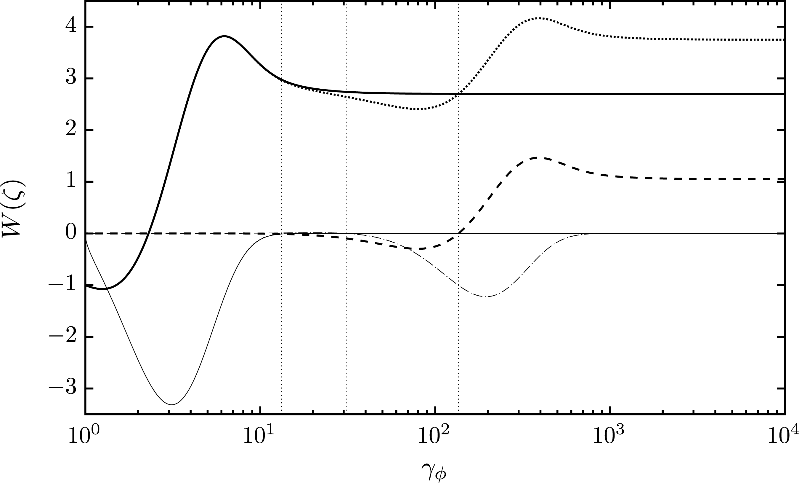
Plots of real (thick) and imaginary (thin) parts of $W(\unicode[STIX]{x1D701})$ (dotted), $W_{0}(\unicode[STIX]{x1D701})$ (solid) and $\unicode[STIX]{x1D700}_{n}\unicode[STIX]{x1D6FE}_{\text{b}}W_{1}(\unicode[STIX]{x1D701})$ (dashed) over $\unicode[STIX]{x1D6FE}_{\unicode[STIX]{x1D719}}$ for $\unicode[STIX]{x1D70C}_{0}=1$ , $\unicode[STIX]{x1D700}_{\unicode[STIX]{x1D70C}}=1$ , $\unicode[STIX]{x1D700}_{n}=10^{-4}$ and $\unicode[STIX]{x1D6FE}_{\text{b}}/\unicode[STIX]{x1D6FE}_{\text{b},\min }=2$ . The three vertical dotted lines indicate, from left to right, $\unicode[STIX]{x1D6FE}_{\unicode[STIX]{x1D719}}=\unicode[STIX]{x1D6FE}_{2},\unicode[STIX]{x1D6FE}_{1},\unicode[STIX]{x1D6FE}|_{\unicode[STIX]{x1D6FD}=\unicode[STIX]{x1D701}_{01}}$ , respectively, with $\unicode[STIX]{x1D6FE}_{1}\approx \unicode[STIX]{x1D6FE}_{\text{b}}$ .

4.3.1 Comparison with ELM

For comparison, the estimate made by ELM for a streaming relativistic Gaussian distribution, $\propto \exp [-(u-u_{\text{b}})^{2}/\langle \unicode[STIX]{x1D6FE}\rangle ^{2}]$ , may be written as

(4.17) $$\begin{eqnarray}2\left(\frac{\unicode[STIX]{x1D714}_{i}}{\unicode[STIX]{x1D714}_{r}}\right)_{\text{rr}}\approx \frac{\sqrt{3}}{\unicode[STIX]{x1D6FE}_{\text{b}}}\frac{(n_{1}/n_{0})^{1/3}}{10\langle \unicode[STIX]{x1D6FE}\rangle _{0}}\sim \frac{10^{-3}}{\langle \unicode[STIX]{x1D6FE}\rangle _{0}^{2}},\end{eqnarray}$$

with $n_{1}/n_{0}\sim 10^{-3}$ and where we use $\unicode[STIX]{x1D6FE}_{\text{b}}\sim 10\langle \unicode[STIX]{x1D6FE}\rangle _{0}$ as in (3.17). We may estimate (4.11) as $\overline{\unicode[STIX]{x1D6E4}}_{\text{rr}}\sim 10^{-2}/\langle \unicode[STIX]{x1D6FE}\rangle _{0}$ for these parameter values. The resonant reactive growth rate for a streaming Gaussian distribution, equation (4.17), is smaller than for a Jüttner distribution, equation (4.11), by a factor ${\sim}1/10\langle \unicode[STIX]{x1D6FE}\rangle _{0}$ .

4.4 Does reactive instability occur?

Our results appear to be implying that reactive instability occurs for Jüttner distributions in a pulsar plasma. We first describe our search for reactive instability, and then discuss the interpretation and implications of our results.

4.4.2 Why is there no reactive instability?

When damping/growth is weak we may write $W(\unicode[STIX]{x1D701})$ using (2.11) as

(4.18) $$\begin{eqnarray}W(\unicode[STIX]{x1D701})=\frac{1}{n_{0}}\int _{-1}^{1}\,\text{d}\unicode[STIX]{x1D6FD}\frac{\text{d}g(u)/\text{d}\unicode[STIX]{x1D6FD}}{\unicode[STIX]{x1D6FD}-\unicode[STIX]{x1D701}},\end{eqnarray}$$

for $W(\unicode[STIX]{x1D701})=W_{0}(\unicode[STIX]{x1D701})+\unicode[STIX]{x1D700}_{n}\unicode[STIX]{x1D6FE}_{\text{b}}W_{1}(\unicode[STIX]{x1D701})$ with $g(u)$ given by (2.4). Interaction of a wave with phase velocity $\unicode[STIX]{x1D701}$ and a particle with velocity $\unicode[STIX]{x1D6FD}$ is resonant if in (4.18) the Cerenkov resonance condition $\unicode[STIX]{x1D6FD}-\unicode[STIX]{x1D701}=0$ is satisfied; the interaction is non-resonant otherwise. Kinetic instability arises from resonant interaction over regions where $\text{sgn}(\unicode[STIX]{x1D701})\text{d}g(u)/\text{d}\unicode[STIX]{x1D6FD}|_{\unicode[STIX]{x1D6FD}=\unicode[STIX]{x1D701}}>0$ and Landau damping occurs when $\text{sgn}(\unicode[STIX]{x1D701})\text{d}g(u)/\text{d}\unicode[STIX]{x1D6FD}|_{\unicode[STIX]{x1D6FD}=\unicode[STIX]{x1D701}}<0$ . Reactive instability may potentially occur over regions where $\text{sgn}(\unicode[STIX]{x1D701})\text{d}g(u)/\text{d}\unicode[STIX]{x1D6FD}|_{\unicode[STIX]{x1D6FD}=\unicode[STIX]{x1D701}}=0$ such as over phases where $g(u)|_{\unicode[STIX]{x1D6FD}=\unicode[STIX]{x1D701}}$ is a zero/non-zero constant, or over regions where $\text{sgn}(\unicode[STIX]{x1D701})\text{d}g(u)/\text{d}\unicode[STIX]{x1D6FD}|_{\unicode[STIX]{x1D6FD}=\unicode[STIX]{x1D701}}$ is non-zero but sufficiently small to be negligible in comparison to growth through reactive instability (if one exists). When $g(u)|_{\unicode[STIX]{x1D6FD}=\unicode[STIX]{x1D701}}=0$ , the interaction of the wave and the particles is non-resonant (as there are no particles with $\unicode[STIX]{x1D6FD}=\unicode[STIX]{x1D701}$ to resonate with the wave) and when $g(u)|_{\unicode[STIX]{x1D6FD}=\unicode[STIX]{x1D701}}$ is a non-zero constant the interaction is resonant. Magneville (Reference Magneville1990a ,Reference Magneville b ) considered a 3-D Jüttner distribution and concluded that temporal reactive growth is not possible when either the background or the beam interact resonantly with the wave; however, spatial reactive growth may be possible. For parameters relevant to pulsars, there is always resonant interaction between waves and particles in a Jüttner distribution. Aside from an exceedingly small neighbourhood of $\unicode[STIX]{x1D6FE}_{\unicode[STIX]{x1D719}}\approx \unicode[STIX]{x1D6FE}_{\text{b}}$ , Landau dissipation dominates any potential reactive growth and the dissipative term cannot be neglected.

The procedure we have employed in treating reactive instability analytically is based on the dispersion equation (4.1), and it seems that this cannot be justified, in the sense that one cannot justify neglecting the beam in determining the wave frequency. The contribution of the beam, which is heavily Landau damped, makes a significant contribution or even dominates the background invalidating the assumption $|\unicode[STIX]{x1D714}_{i}/\unicode[STIX]{x1D714}|\ll 1$ . In effect, Landau damping dominates over reactive growth, invalidating the latter. We conclude that the conventional concept of a reactive instability does not apply for a Jüttner distribution for parameter values relevant to pulsars.

5.1 Temporal and spatial growth

The kinetic equation for growing waves is of the form of a total derivative, $D/Dt=\unicode[STIX]{x2202}/\unicode[STIX]{x2202}t+\boldsymbol{v}_{\text{g}}\boldsymbol{\cdot }\unicode[STIX]{x1D735}$ where $\boldsymbol{v}_{\text{g}}$ is the group velocity, operating on the wave amplitude equal to $\unicode[STIX]{x1D6E4}$ times the wave amplitude, where $\unicode[STIX]{x1D6E4}$ is the growth rate calculated using dispersion theory. In the 1-D case discussed here one has $\boldsymbol{v}_{\text{g}}\boldsymbol{\cdot }\unicode[STIX]{x1D735}=\unicode[STIX]{x1D6FD}_{\text{g}}c\unicode[STIX]{x2202}/\unicode[STIX]{x2202}s$ , where $\unicode[STIX]{x1D6FD}_{\text{g}}$ is the group speed and $s$ is distance along the ray path. Temporal and spatial growth may be described by imaginary parts, $\text{Im}\,\unicode[STIX]{x1D714}$ and $\text{Im}\,k_{\Vert }$ , of the frequency and (parallel) wavenumber, respectively, with the amplitude varying $\propto \exp (\text{Im}\,\unicode[STIX]{x1D714}\,t-\text{Im}\,k_{\Vert }\,s)$ . The ratio of temporal and spatial terms depends partly on the boundary conditions: waves uniformly excited everywhere grow only in time and waves excited at a point source grow only in space away from the source. One has $\text{Im}\,\unicode[STIX]{x1D714}=\unicode[STIX]{x1D6E4},\text{Im}\,k_{\Vert }=0$ for purely temporal growth and $\text{Im}\,\unicode[STIX]{x1D714}=0,\text{Im}\,k_{\Vert }=-\unicode[STIX]{x1D6E4}/c\unicode[STIX]{x1D6FD}_{\text{g}}$ for purely spatial growth.

A helpful step in relating temporal and spatial growth in different frames is to consider the frame in which the group speed is zero. In this frame the wave energy is not propagating, and wave growth must be purely temporal. In the plasma rest frame, the group velocity may be directed either outward or inward. Let us use labels $g\pm$ to denote these cases, writing the group velocity as $\pm c\unicode[STIX]{x1D6FD}_{\text{g}}$ , with $\unicode[STIX]{x1D6FD}_{\text{g}}$ defined to be positive. There are then two frames ${\mathcal{K}}_{\text{g}\pm }$ , defined by the group velocity being zero for waves that are propagating outward and inward in ${\mathcal{K}}$ , respectively. Let $t_{\text{g}\pm }$ and $s_{\text{g}\pm }$ be time and distance in ${\mathcal{K}}_{\text{g}\pm }$ . One has

(5.1a,b ) $$\begin{eqnarray}t_{\text{g}\pm }=\unicode[STIX]{x1D6FE}_{\text{g}}(t\pm \unicode[STIX]{x1D6FD}_{\text{g}}s/c),\quad s_{\text{g}\pm }=\unicode[STIX]{x1D6FE}_{\text{g}}(s\pm \unicode[STIX]{x1D6FD}_{\text{g}}ct),\end{eqnarray}$$

where $\unicode[STIX]{x1D6FE}_{\text{g}}=(1-\unicode[STIX]{x1D6FD}_{\text{g}}^{2})^{-1/2}$ is the Lorentz factor corresponding to the group speed. The exponent in the variation of the amplitude, $\propto \exp (\text{Im}\,\unicode[STIX]{x1D714}\,t-\text{Im}\,k_{\Vert }\,s)$ , is an invariantFootnote ³ , and may be rewritten as a variation $\propto \exp (\unicode[STIX]{x1D6E4}t_{\text{g}\pm }/\unicode[STIX]{x1D6FE}_{\text{g}})$ .

5.2 Growth in the pulsar frame

The growth rate in the pulsar frame ${\mathcal{K}}^{\prime }$ is related to the growth rate in the rest frame of the plasma by a Lorentz transformation applied to $\text{Im}\,\,\unicode[STIX]{x1D714}$ , $\text{Im}\,\,k_{\Vert }$ , $t$ and $s$ in ${\mathcal{K}}$ to $\text{Im}\,\,\unicode[STIX]{x1D714}^{\prime }$ , $\text{Im}\,\,k_{\Vert }^{\prime }$ , $t^{\prime }$ and $s^{\prime }$ in ${\mathcal{K}}^{\prime }$ . The direct transforms are

(5.2) $$\begin{eqnarray}\left.\begin{array}{@{}c@{}}\text{Im}\,\,\unicode[STIX]{x1D714}^{\prime }=\unicode[STIX]{x1D6FE}_{\text{s}}(\text{Im}\,\,\unicode[STIX]{x1D714}+\unicode[STIX]{x1D6FD}_{\text{s}}\text{Im}\,\,k_{\Vert }c),\quad \text{Im}\,\,k_{\Vert }^{\prime }=\unicode[STIX]{x1D6FE}_{\text{s}}(\text{Im}\,\,k_{\Vert }+\unicode[STIX]{x1D6FD}_{\text{s}}\text{Im}\,\,\unicode[STIX]{x1D714}/c),\\ t^{\prime }=\unicode[STIX]{x1D6FE}_{\text{s}}(t+\unicode[STIX]{x1D6FD}_{\text{s}}s/c),\quad s^{\prime }=\unicode[STIX]{x1D6FE}_{\text{s}}(s+\unicode[STIX]{x1D6FD}_{\text{s}}ct),\end{array}\right\}\end{eqnarray}$$

and the inverse transforms follow by interchanging primed and unprimed quantities and replacing $\unicode[STIX]{x1D6FD}_{\text{s}}$ by $-\unicode[STIX]{x1D6FD}_{\text{s}}$ . The group speeds $\pm \unicode[STIX]{x1D6FD}_{\text{g}}$ in ${\mathcal{K}}$ transform into

(5.3) $$\begin{eqnarray}\unicode[STIX]{x1D6FD}_{\text{g}\pm }^{\prime }=\frac{\pm \unicode[STIX]{x1D6FD}_{\text{g}}+\unicode[STIX]{x1D6FD}_{\text{s}}}{1\pm \unicode[STIX]{x1D6FD}_{\text{g}}\unicode[STIX]{x1D6FD}_{\text{s}}}\end{eqnarray}$$

in ${\mathcal{K}}^{\prime }$ . With the variation of the amplitude $\propto \exp (\text{Im}\,\unicode[STIX]{x1D714}^{\prime }\,t^{\prime }-\text{Im}\,k_{\Vert }^{\prime }\,s^{\prime })$ in ${\mathcal{K}}^{\prime }$ , one identifies $\text{Im}\,\unicode[STIX]{x1D714}^{\prime }=\unicode[STIX]{x1D6FE}_{\text{g}\pm }^{\prime }\unicode[STIX]{x1D6E4}$ , $\text{Im}\,k_{\Vert }^{\prime }=-\unicode[STIX]{x1D6FE}_{\text{g}\pm }^{\prime }\unicode[STIX]{x1D6E4}/c\unicode[STIX]{x1D6FD}_{\text{g}\pm }^{\prime }$ with $\unicode[STIX]{x1D6FE}_{\text{g}\pm }^{\prime }=\unicode[STIX]{x1D6FE}_{\text{s}}\unicode[STIX]{x1D6FE}_{\text{g}}(1\pm \unicode[STIX]{x1D6FD}_{\text{g}}\unicode[STIX]{x1D6FD}_{\text{s}})$ , and with $\unicode[STIX]{x1D6E4}$ calculated in ${\mathcal{K}}$ by setting $\text{Im}\,k_{\Vert }=0$ and $\unicode[STIX]{x1D6E4}=\text{Im}\,\unicode[STIX]{x1D714}$ .

5.3 Growth factor

The growth factor, $G$ , such that the wave amplitude increases by a factor $\exp (G)$ during the wave growth, is an invariant. Suppose that (constant) wave growth starts at one event and finishes at another event, with the two events separated by $\unicode[STIX]{x0394}t,\unicode[STIX]{x0394}s$ in ${\mathcal{K}}$ and by $\unicode[STIX]{x0394}t^{\prime },\unicode[STIX]{x0394}s^{\prime }$ in ${\mathcal{K}}^{\prime }$ . Then one has

(5.4) $$\begin{eqnarray}G=\text{Im}\,\unicode[STIX]{x1D714}\unicode[STIX]{x0394}t-\text{Im}\,k_{\Vert }\unicode[STIX]{x0394}s=\text{Im}\,\unicode[STIX]{x1D714}^{\prime }\unicode[STIX]{x0394}t^{\prime }-\text{Im}\,k_{\Vert }^{\prime }\unicode[STIX]{x0394}s^{\prime },\end{eqnarray}$$

which allows one to estimate the growth factor by applying appropriate boundary conditions in either frame.

One restriction on $G$ arises from the spatial variation of the number density $n^{\prime }\propto 1/r^{3}$ in the pulsar magnetosphere. This implies a characteristic distance $L_{\Vert }\approx 3r/2$ over which the plasma frequency $\unicode[STIX]{x1D714}_{\text{p}}^{\prime }$ changes. (In the widely favoured ‘sparking’ model, $L_{\Vert }$ is much smaller, of the order of the size of the cloud of pairs produced in a single spark.) A wave growing in a bandwidth $\unicode[STIX]{x0394}\unicode[STIX]{x1D714}_{\text{bw}}^{\prime }$ in ${\mathcal{K}}^{\prime }$ moves out of resonance, and ceases growing, after propagating a distance $\unicode[STIX]{x0394}s^{\prime }=(\unicode[STIX]{x0394}\unicode[STIX]{x1D714}_{\text{bw}}^{\prime }/\unicode[STIX]{x1D714}^{\prime })L_{\Vert }$ . The foregoing results then enable one to estimate $G$ . The estimate is quite different for waves propagating outward and inward in ${\mathcal{K}}$ , both of which are propagating outward in ${\mathcal{K}}^{\prime }$ for $\unicode[STIX]{x1D6FD}_{\text{s}}>\unicode[STIX]{x1D6FD}_{\text{g}}$ . For $\unicode[STIX]{x1D6FE}_{\text{s}}\gg \unicode[STIX]{x1D6FE}_{\text{g}}$ one has $\unicode[STIX]{x1D6FE}_{\text{g}+}^{\prime }\approx 2\unicode[STIX]{x1D6FE}_{\text{s}}\unicode[STIX]{x1D6FE}_{\text{g}}$ and $\unicode[STIX]{x1D6FE}_{\text{g}-}^{\prime }\approx \unicode[STIX]{x1D6FE}_{\text{s}}/2\unicode[STIX]{x1D6FE}_{\text{g}}$ , implying that the spatial growth rate, $\unicode[STIX]{x1D6FE}_{\text{g}\pm }^{\prime }\unicode[STIX]{x1D6E4}/c$ , is of order $\unicode[STIX]{x1D6FE}_{\text{s}}^{2}$ larger for outward than for inward-propagating waves in ${\mathcal{K}}$ . The frequencies in ${\mathcal{K}}^{\prime }$ are also quite different, $\unicode[STIX]{x1D714}_{+}^{\prime }\approx 2\unicode[STIX]{x1D6FE}_{\text{s}}\unicode[STIX]{x1D714}$ and $\unicode[STIX]{x1D714}_{-}^{\prime }\approx \unicode[STIX]{x1D714}/2\unicode[STIX]{x1D6FE}_{\text{s}}\unicode[STIX]{x1D6FE}_{\unicode[STIX]{x1D719}}^{2}$ for $\unicode[STIX]{x1D6FE}_{\text{s}}^{2}\gg \unicode[STIX]{x1D6FE}_{\unicode[STIX]{x1D719}}^{2}$ . As a result the fractional growth rate in ${\mathcal{K}}^{\prime }$ is approximately equal to the fractional growth rate in ${\mathcal{K}}$ for outward-propagating waves, but for inward propagating waves it is larger by a factor of order $\unicode[STIX]{x1D6FE}_{\text{s}}^{2}\unicode[STIX]{x1D6FE}_{\unicode[STIX]{x1D719}}^{2}/\unicode[STIX]{x1D6FE}_{\text{g}}^{2}$ . A detailed comparison of these two cases is needed, and we plan to discuss these details elsewhere. Suffice it to say here, neither seems favourable as a basis for pulsar radio emission.