


1. Introduction
Exporters from developing countries face substantial costs in reaching and maintaining foreign customers. A growing literature shows that heterogeneity in firms’ customer bases can account for important trade patterns, including pricing and market penetration (Arkolakis Reference Arkolakis2010; Bernard et al. Reference Bernard, Moxnes and Ulltveit-Moe2018b; Alviarez et al. Reference Alviarez, Fioretti, Kikkawa and Morlacco2023). In this paper, we show that firms can mitigate these product-market frictions in international markets by outsourcing production domestically. We develop an equilibrium model to quantify how domestic outsourcing relaxes customer-capital constraints for exporters and, in turn, improves aggregate efficiency.
Our study is based on a unique dataset that links the production and sales activities of Chinese exporting firms. We document a systematic wedge between the value of goods a firm produces for export and the value of goods it sells in foreign markets. In 2006, more than 62% of Chinese exporters sold an amount that differed from what they produced. Moreover, for firms whose production-to-sales ratio differs from one, the gap is economically large: the value difference between production and sales amounts to 22% of total exports in 2006. This pattern appears even within narrowly defined homogeneous industries and cannot be explained by measurement error, exchange-rate fluctuations, processing trade, or inventory management. We interpret this evidence as indicating that some producers also act as trade intermediaries, particularly those that export more than they produce. We refer to such firms as “producer intermediaries.”
Our analysis further indicates that firms with greater marketing expenditures are more likely to export more than they produce, conditional on productivity. This result is robust across alternative specifications and estimation methods. Interpreting accumulated marketing expenditure as a proxy for customer capital, we uncover a strong link between customer capital and the production-to-sales ratio. In particular, firms with higher customer capital are more likely to function as producer intermediaries.
To interpret our empirical findings, we develop a theoretical framework in which the difficulty of reaching foreign customers is summarized by a firm-level state variable, which we call customer capital. The model allows firms to “lend” and “borrow” customer capital through outsourcing relationships. Firms decide whether to become direct exporters on the basis of their productivity and foreign customer capital. Entry into direct exporting requires paying a fixed cost, and firms’ ability to serve foreign markets is constrained by their stock of customer capital. Firms with a large customer base can outsource part of their production to other direct exporters or to domestic producers that are more efficient in production but lack sufficient customer capital. In this way, outsourcing allows firms with limited customer capital to access foreign markets without bearing the full cost of establishing foreign customer relationships.
The outsourcing price is determined in equilibrium so that aggregate demand and supply in the outsourcing market are equalized. To capture frictions in the outsourcing process, we introduce an additional outsourcing cost on top of the market price and estimate its magnitude using our data. A key feature of the model is that it accommodates two types of outsourcing firms: pure intermediaries, which do not produce export goods themselves, and producer intermediaries, which both produce and export. The framework therefore extends the standard model of trade intermediaries, which focuses exclusively on pure intermediaries.
A good institutional example comes from China’s textile and apparel export regime prior to the abolition of the Multifiber Arrangement (MFA) in 2005. Under this regime, export quotas and licenses were administratively allocated, so access to foreign buyers could be separated from production capability. As discussed by Yang (Reference Yang1999), firms without direct quota access could reach export markets by subcontracting to enterprises that held quotas, and such arrangements were not uncommon in practice. Yang also notes that China’s textile and clothing quota allocation regime favored large SOEs in the coastal regions. This institutional setting is consistent with our interpretation of customer capital as market access or buyer access that is distinct from production capability and may induce outsourcing or subcontracting.
We calibrate the model using data from the textile and apparel industry, where goods are relatively homogeneous. We then use the calibrated model to quantify the role of outsourcing in international trade. Our results show that, although frictions prevent firms from outsourcing efficiently, outsourcing still delivers substantial gains in aggregate industry productivity. Absent outsourcing, aggregate productivity in the industry would be 7.85% lower. Without the ability to outsource, firms with high customer capital but low productivity are unable to fully utilize their access to foreign demand, which reduces aggregate supply and lowers the equilibrium volume of exports.
We investigate the role of the joint distribution of customer capital and firm productivity in determining aggregate industry productivity. We find a strong positive association between the two variables: the estimated correlation between log customer capital and log productivity is 0.79. We then consider a counterfactual in which the correlation is perfect and equal to one. In this case, aggregate productivity increases by 4.5%. The result highlights a potential source of inefficiency: when low-productivity firms accumulate high customer capital, they must rely heavily on outsourcing to serve foreign markets. Our findings further suggest that policies aimed at promoting export-market entry may be more effective when directed toward high-productivity firms.
We next examine whether the gains from reducing the entry cost differ depending on whether outsourcing is available. Our results show that a 10% reduction in the entry cost raises aggregate industry productivity by 2.12% when outsourcing is allowed, compared with 5.4% when it is not. The reason is that, with outsourcing, domestic firms can already serve foreign markets indirectly by producing for direct exporters. Consequently, when entry costs fall and some firms begin to export directly, the incremental productivity gains are smaller than in an environment without outsourcing, where non-exporting firms are unable to contribute to export production at all. This result highlights the importance of incorporating outsourcing when assessing the aggregate effects of lower entry costs in the presence of customer-capital frictions. Absent this margin, the gains from reducing entry costs may be overstated. More generally, the result suggests that firms’ ability to reorganize production through outsourcing can mitigate the effects of changes in trade barriers.
In our final counterfactual, we assess the role of producer intermediaries in accounting for our results. We consider an economy in which only pure intermediaries are allowed to intermediate trade. Relative to the benchmark, aggregate productivity falls by 4.51%, indicating that producer intermediaries are quantitatively important for aggregate efficiency in international trade. For comparison, removing intermediaries altogether—thereby eliminating outsourcing—lowers aggregate productivity by 7.85%. Thus, more than half of the total productivity loss from shutting down intermediation is attributable to the absence of producer intermediaries. Their role remains quantitatively important even when the entry cost is reduced by 10%.
The paper contributes to two streams of literature. Firstly, it has been pointed out that due to friction in the product market, the customer base has a large impact on individual firm performance as well as aggregate efficiency (Foster et al. Reference Foster, Haltiwanger and Syverson2016; Gourio and Rudanko Reference Gourio and Rudanko2014; Luttmer et al. Reference Luttmer2006; Pozzi and Schivardi Reference Pozzi and Schivardi2016). Specifically, the friction in reaching foreign customers on the international market is much bigger than that in the domestic market. For instance, Drozd and Nosal (Reference Drozd and Nosal2012) develop a model of search frictions in the exporting market and show building a customer base in the exporting market is the key to understanding the price dynamics of exporting goods. Relatedly, Arkolakis (Reference Arkolakis2010) develops a model of a marketing cost in the exporting market (in the presence of search friction) as a specific trade cost and shows the model can reconcile many features of exporting firms’ dynamics. Our paper builds on this stream of research, emphasizing that exporters can alleviate the high costs of reaching and maintaining foreign customers via outsourcing and quantifying the importance of this channel. We find that the friction in the export product market may not be as important as suggested by the previous literature.
Secondly, our paper contributes to the research about trade intermediaries. The significance of Chinese trade intermediary firms in enabling international trade has been well documented (Ahn et al. Reference Ahn, Khandelwal and Wei2011; Bai et al. Reference Bai, Krishna and Ma2017). Similarly, Blum et al. (Reference Blum, Claro, Dasgupta, Horstmann and Rangel2023) show that trade intermediaries play an important role in Chile. However, these papers focus on firms which are specialized in intermediary services. Our paper points out that most indirect trade is carried by firms that are producers as well. We find that these producers’ behaviors can significantly change the equilibrium outsourcing price, hence changing the efficiency of the aggregate market. In a related paper, Bernard et al. (Reference Bernard, Blanchard, Van Beveren and Vandenbussche2018a) have also noticed this significant pattern, which the authors named “carry-along trade.” The paper interprets this phenomenon as reflecting the fact that products with complementarities (such as desks and chairs) are better sold together. We find that even in an industry with relatively homogeneous products, this phenomenon still exists. Our paper therefore complements their findings.
The paper is organized as follows. Section 2 documents motivating facts for this study. Section 3 presents a model of outsourcing in international trade. The quantitative results are shown in Section 4. Section 5 concludes.
2. Motivating facts
In this section, we provide an overview of the dataset used in this study and present the key empirical findings.
2.1 Data
To construct the main sample, we merged the Annual Surveys of Industrial Production in China (ASIP) with Chinese customs data from 2000 to 2006. The ASIP dataset includes all manufacturing firms, whether state-owned or privately owned, with annual sales exceeding 5 million RMB (equivalent to 0.71 million USD).Footnote 1 In addition to a firm’s characteristics, the ASIP provides information on the value of export goods that the firm produced. This variable captures both the value of export goods that are directly sold by the surveyed firm and the value of export goods that are sold through other channels.Footnote 2 The Chinese customs data contain a firm’s export value, price, and destination information of each product in the 6-digit Harmonized System (HS6) at the transaction level. The customs data only record the firms that carry the goods abroad. As a result, some exporters in the customs data may be trade intermediaries or manufacturing firms that carry products that they do not produce.
The aggregate export values in the two datasets are comparable. As shown in Table 1, the aggregate export values in the ASIP are about 80% of the aggregate export values in the Chinese customs data in all years. The 20% gap is likely due to the ASIP not covering small firms whose annual sales are less than 5 million RMB.
Total export values from the ASIP and the customs data

Table 1. Long description
A table comparing total export values from the ASIP and customs data over the years 2000 to 2006. The table has 7 rows and 4 columns. Column headers are Year, ASIP, Customs data, and a percentage value. Row labels are the years from 2000 to 2006. Row 1: Year 2000, ASIP 1,460, Customs data 1,880, Percentage 78. Row 2: Year 2001, ASIP 1,610, Customs data 2,020, Percentage 80. Row 3: Year 2002, ASIP 2,010, Customs data 2,510, Percentage 80. Row 4: Year 2003, ASIP 2,700, Customs data 3,390, Percentage 80. Row 5: Year 2004, ASIP 4,050, Customs data 4,600, Percentage 88. Row 6: Year 2005, ASIP 4,770, Customs data 5,990, Percentage 80. Row 7: Year 2006, ASIP 6,050, Customs data 7,630, Percentage 80. The table shows that the ASIP values are consistently about 80% of the customs data values, with a notable increase in both datasets over the years.
Note: This table shows the total export values from the ASIP and customs data for each year before merging the two datasets. Unit: one billion CNY.
Given that the two datasets do not share the same firm identifier, we impose strict criteria when we match firms in the two datasets following Bai et al. (Reference Bai, Krishna and Ma2017). Based on (1) firm name, (2) region code, (3) address, (4) phone number, and (5) legal representative, two firms in each dataset are classified as the same firm only if a majority of that information is matched. Bai et al. (Reference Bai, Krishna and Ma2017) conduct several robustness checks for their matching criteria that we follow in this study and find the matching criteria reliable.
Of 405,374 firm-year observations for firms in the ASIP that produced export goods, about 48% (194,072) are in the Chinese customs data.Footnote 3 For the firms shown in both the ASIP and the customs data, we compare the value of export goods that a firm produced, as contained in the ASIP, and the value of goods that the firm exported, as contained in the customs data. For convenience, we call the value of export goods that a firm produced in the ASIP the “production” value and the value of goods that the firm exported in the customs data the “sales” value.
2.2 Main findings
The main motivating fact for this paper is shown in Figure 1. It shows the histogram for the log value of production per sales for all firm-year observations. We observe a substantial variation in exporting firms’ production-per-sales value. Relatively more mass is observed around zero, but many firms exhibit either negative or positive log production-per-sales value. In other words, many firms are exporting more or less than what they produce for export.Footnote 4
Number of firms conditional on production per sales (
 $s$
)

Table 2. Long description
A table titled ‘Number of firms conditional on production per sales ()’ with data spanning from 2000 to 2006. The table has four columns: Year, Number (Share) of firms s ∈ (0.9, 1.1) (%), Number (Share) of firms s ∈ (0, 0.9) (%), Number (Share) of firms s ∈ [1.1, ∞) (%), and Total. Each row lists the year and the corresponding number and share of firms in three different production per sales ranges, along with the total number of firms for that year. The table shows an increase in the total number of firms over the years, with notable variations in the share of firms across different production per sales ranges.
Note: This table shows the number (and proportion) of firms conditional on production per sales
 $s=\frac {\text{Production value}}{\text{Sales value}}$
.
Histogram for Log production per sales: all industries.
Note: This figure shows the histogram for the log value of production per sales for those with a positive sales value.

To control measurement errors, we allow 10% error bounds for the production-per-sales value and report the number of firms that export different amounts that they produced.Footnote 5 Table 2 shows the specific number (and the proportion) of firms for the production-per-sales value each year. Consistent with Figure 1, exporting firms’ sales value is often different from their production value. For example, more than 62% of Chinese exporting firms sold more or less than what they produced in 2006. Thus, we conclude that the difference between the production and sales values is not driven by measurement errors.
Some domestic firms import all the necessary parts to produce final goods, assemble them, and export them as final products. Often referred to as “processing trade,” this type of trade is common in China (Yu and Tian Reference Yu, Tian, McKay and Song2012). Product-level information on processing trade is available in the customs data but not in the ASIP. To examine whether the main pattern in the data is primarily driven by firms engaged in processing trade, we remove all firm-year observations involving processing trade and plot the histogram of the log production-to-sales ratio in Figure 2. The main pattern remains, suggesting that our empirical findings are not primarily driven by processing trade.
Histogram for Log production per sales: excluding processing trade.
Note: This figure shows the histogram for the log value of production per sales, excluding firm-year observations involved with the processing trade.

Another explanation could be that firms do not ship all the goods produced in the current period and store some of them as inventory to export in the next period. To address the possibility that inventory management drives the observed discrepancies between production and sales, we aggregated each firm’s export values from both the Annual Survey of Industrial Production (ASIP) and the customs data across the entire sample period. By constructing a ratio of total aggregated production value to total aggregated sales value for each firm, we effectively net out year-by-year inventory fluctuations. As illustrated in the histogram of this long-run measure (Figure 3), the distribution remains remarkably consistent with the annual patterns previously documented. This suggests that temporal adjustments and inventory storage within firms are unlikely to account for the substantial and persistent dispersion in the production-per-sales ratio.
Overall, we conclude that the empirical pattern we have observed reflects the fact that some producers are functioning as intermediaries, especially those that export more than they produce. Before examining the reasons why some producers act as intermediaries, we analyze the value difference between production and sales, particularly for firms whose production per sales differs from one. In Table 3, we have calculated the aggregate (absolute) value difference for two groups: (1) firms whose production per sales is less than 0.9 and (2) firms whose production per sales is greater than 1.1. The value difference between production and sales for these two groups was 1,661 billion CNY in 2006, which is comparable to 22% of the aggregate customs value for that year.
Note that the mass of firms whose production exceeds their sales is considerably larger than that of firms with the reverse pattern. This asymmetry arises because, while our sample covers most of the firms with
 $s\geq 1.1$
, the corresponding excess sales are split between producer intermediaries, which are in the sample, and pure intermediaries, which are not manufacturing firms and therefore fall outside our sample.
Value difference between production and sales

Table 3. Long description
A table comparing value differences between production and sales for two groups of firms over several years. The table has 7 rows and 4 columns. The columns are labeled as follows: Year, (1) s ∈ (0, 0.9), and (2) s ∈ [1.1, ∞). The row labels are the years from 2000 to 2006. The values in the table are as follows: Row 1: 2000, 62, 308. Row 2: 2001, 71, 344. Row 3: 2002, 88, 441. Row 4: 2003, 177, 600. Row 5: 2004, 236, 761. Row 6: 2005, 355, 986. Row 7: 2006, 451, 1,210.
Note: This table shows the aggregate value difference between production and sales (
 $|\text{production}-\text{sales}|$
) for firms with
 $s\lt 0.9$
and
 $s\gt 1.1$
. Unit: one billion CNY.
Histogram of the Log ratio of total production to total sales.
Note: This figure shows the ratio of aggregated production value to aggregated sales value for each firm over time.

2.3 Comparison to the previous findings
Using Belgian customs data, Bernard et al. (Reference Bernard, Blanchard, Van Beveren and Vandenbussche2018a) observed a data pattern similar to what we have found. Specifically, they demonstrated that firms frequently export a wider range of products than they produce, which they referred to as “Carry-Along Trade.” They also found that exporting firms could increase the price of their regular products by pairing them with products they did not produce themselves and showed that product complementarity accounts for the trade pattern they identified.Footnote 6
First of all, we provide evidence of carry-along trade in China, suggesting that the practice of firms exporting more than they produce may be widespread and not confined to a specific country. Second, while the motive of complementarity among export goods can explain some of the variations in the data, we argue that it may not be the sole reason for the observed pattern. For example, even in industries with highly substitutable products such as cotton and chemical fiber or textile and garment manufacturing, the variation in production per sales remains prevalent. Figure 4 illustrates the log value of production per sales for the textile and garment industry, where products are relatively similar. We observe significant variation in the production-per-sales value, even among firms that produce comparable goods. This finding suggests that the complementarity story may not fully explain the observed variation.
Number of firms conditional on core sales

Table 4. Long description
A table showing the number of firms with core sales greater or less than production from 2000 to 2006. The table has two columns and seven rows, including the header row. Column headers are ‘Core sales > production (%)’ and ‘Core sales ≤ production (%)’. Row labels are the years from 2000 to 2006. Each cell contains the number of firms and the proportion in percent. Row 1: 2000, 872 (39), 1,378 (61). Row 2: 2001, 1,027 (40), 1,574 (60). Row 3: 2002, 1,197 (39), 1,908 (61). Row 4: 2003, 1,363 (39), 2,152 (61). Row 5: 2004, 1,905 (38), 3,106 (62). Row 6: 2005, 2,017 (37), 3,503 (63). Row 7: 2006, 2,344 (35), 4,383 (65). The table shows that the number of firms with core sales greater than production increases over the years, while the proportion decreases. Conversely, the number of firms with core sales less than or equal to production also increases, with a slight increase in proportion.
Note: This table shows the number (and proportion) of two types of firms among exporters whose sales value is greater than their production value. The core-sales value is the sales value (recorded at customs data) of goods categorized within the manufacturing survey’s registered industry.
Histogram for log production per sales: textile and garment production.
Note: This figure shows the histogram for the log value of production per sales for the textile and garment industry.

To show this point further, we separate the sales of HS6 products into two groups: HS6 products within firms’ four-digit registered industry in ASIP data (which we call “core sales”) and other HS6 products. We then further categorize firms that export more than they produce into two types: (1) firms whose core sales are greater than their production and (2) firms whose core sales are less than or equal to their production. Core products, which are within a four-digit industry, are more likely to be substitutable than complementary. Table 4 shows that among firms whose production per sales is less than 0.9, about one-third of firms export more core products than they produce.
The ASIP categorizes a firm into a four-digit industry code, depending on the products that the firm produces. On the other hand, HS6 product codes are a more refined categorization than four-digit Chinese industry codes for some industries. Readers may worry that even within a homogeneous industry, many different products may still complement each other (e.g., an article of clothing may need different textiles). To handle this concern, we focus on 4-digit Chinese industries in which only one HS6 product is categorized. The number of HS6 products assigned to each Chinese industry varies across industries. Some industries contain only one HS6 product, mapping the industry code and HS6 product code one to one. The concern is less severe in those industries.Footnote 7 Figure 5 shows the log value of production per sales for those one-product industries. We still observe many firm-year (in this case, firm-product-year) observations in which production and sales values are significantly different.
Histogram for Log production per sales: industries with one HS6 product.
Note: This figure shows the histogram for the log value of production per sales for industries in Table 5.

Our focus on the organizational choice between production and outsourcing relates to recent research on the role of intermediaries in production networks. For instance, Blum et al. (Reference Blum, Claro, Dasgupta, Horstmann and Rangel2023) use a Chilean dataset to show that wholesalers facilitate trade by allowing productive foreign suppliers to reach a broad base of domestic firms, thereby reducing the high relationship costs of international trade. While Blum et al. (Reference Blum, Claro, Dasgupta, Horstmann and Rangel2023) emphasize the role of pure wholesalers in linking producers to markets, our paper highlights that producers themselves often fulfill this intermediary role.
The list of Chinese industries with one HS6 product

Table 5. Long description
A table titled ‘The list of Chinese industries with one HS6 product’ contains two columns: Industry code and Industry name. The table has 50 rows, each representing a different industry. The first column lists the industry codes, and the second column lists the corresponding industry names. The industries range from Aquatic feed manufacturing to Manufacturing of coal products.
2.4 Production-sales ratio and marketing expenditure
In this section, we aim to provide a better understanding of Chinese exporting firms’ carry-along trade by documenting key empirical patterns associated with this phenomenon. In particular, we show that a firm’s accumulated marketing expenditure is strongly associated with the firm’s production-sales ratio.
In Table 6, we present the transition probabilities of intermediation modes for Chinese exporting firms. To facilitate the analysis, we classify the firms into three groups based on the ratio of their sales value to production value: (1) firms with higher sales value than production value (
 $s\in (0,0.9]$
), (2) firms whose production and sales have similar values (
 $s\in (0.9,1.1)$
), and (3) firms with higher production value than sales value (
 $s\in [1.1,\infty )$
). Firms in the first group produce exporting goods themselves but also act as trade intermediaries for other exporting firms, and we refer to them as “producer intermediaries.” Firms in the second group do not rely on trade intermediaries, while firms in the third group use trade intermediaries to export their products. The transition matrix reveals that the probability of a firm remaining in its current production-sales mode in the next period is considerably higher than the probability of it switching to another mode, indicating that firms’ production-sales modes are persistent.
Transitions of intermediation modes

Table 6. Long description
A table with three rows and three columns showing transition probabilities of intermediation modes for Chinese exporting firms. The rows are labeled with different ranges of the ratio of sales value to production value: (1) s ∈ (0, 0.9), (2) s ∈ (0.9, 1.1), and (3) s ∈ [1.1, ∞). The columns are labeled with the same ranges for time t. Row 1: s ∈ (0, 0.9), 0.50, 0.28, 0.22. Row 2: s ∈ (0.9, 1.1), 0.12, 0.64, 0.24. Row 3: s ∈ [1.1, ∞), 0.07, 0.20, 0.73.
Note: This table shows the transition probability for each intermediation mode.
 $s=\frac {\text{Production value}}{\text{Sales value}}$
.
Production per sales and marketing expenditure

Table 7. Long description
A table with seven columns and eleven rows, presenting regression estimates for the production-per-sales ratio and its relationship with marketing expenditure. The columns are labeled as (1), (2), (3), (4), (5), (6), and (7), with the last two columns representing Pure indirect exporter and Indirect exporter. The rows list variables such as ln(acc. marketing), ln(TFP), ln(Firm size), Year FE, Year-Ind. FE, Year-Ind.-Des. FE, Firm FE, Pure exporter, Sole destination, Observations, and R-squared. Each cell contains numerical values and standard errors in parentheses. Notable trends include significant positive relationships between ln(acc. marketing) and the production-per-sales ratio across different columns, with varying degrees of significance indicated by asterisks. The table also shows the number of observations and R-squared values for each regression model.
Note: This table shows regression estimates for the production-per-sales ratio and its relationship with marketing expenditure. Columns (1) through (5) use the log value of production per sales as the dependent variable. The main destination of a firm (Des.) is defined as the country with the highest sales value in a given year. Industry refers to the 4-digit registered industry in the Annual Survey of Industrial Production (ASIP), and firm size is measured by the number of employees. ln(acc. marketing) denotes the log value of accumulated marketing expenditure. Pure exporter refers to firms with zero domestic sales, and Sole Destination refers to firms exporting to only one country. In columns (6) and (7), the dependent variables are dummy variables representing different tiers of intermediation: “Pure indirect exporter” is equal to one for firms that produce export goods but do not appear in the customs data, while “Indirect exporter” includes all firms whose production values exceed their sales values, including pure indirect exporters.
In Table 7, we present the regression results for the log value of production per sales on firms’ accumulated marketing expenditure. In the first column, we control for the year-industry fixed effect in addition to log TFP and firm size. The industry refers to the core industry reported in the ASIP. For two exporting firms in the same industry and the same year, if a firm’s accumulated marketing expenditure is 10% higher, its production per sales is about 0.7% lower. In the second column, we further control for the firm’s main destination—defined as the country with the highest export value—to compare firms within the same industry, year, and destination. This control is particularly important to address the possibility that global demand fluctuations drive the discrepancies between production and sales. If these patterns were merely temporary mismatches caused by goods originally intended for export being redirected to the domestic market, the significance of marketing expenditure would likely diminish. However, the coefficient remains negative and significant, suggesting that the observed discrepancies reflect stable organizational choices rather than short-run demand volatility. In the third column, we control for the firm fixed effect. Consistent with the previous findings, a 10% increase in the aggregated marketing expenditure for a given firm leads to about a 1% decrease in its production per sales.
Note that since marketing expenditure is a firm-level variable, it may capture a firm’s general tendency to invest in its product or firm brands and thus could be used to attract domestic customers as well. In column (4) of Table 7, we restrict our sample to exporting firms that do not sell domestically, and even among these “pure” exporters, we find a clear negative relationship between accumulated marketing expenditure and the production-per-sales ratio. In column (5) of Table 7, we further restrict our sample to pure exporters that sell in only one foreign market, and the main result remains consistent.
To address concerns regarding non-matched firms and the potential distortion of empirical results, we expand our analysis to include firms that appear in the manufacturing survey as producers of export goods but are absent from the customs data. These entities represent firms that produce export goods but do not export directly, likely relying on intermediaries or other direct exporters to reach foreign markets. We examine whether these firms exhibit lower levels of marketing expenditure compared to those that maintain direct access to foreign customers. In column (6), the dependent variable is a “Pure indirect exporter” dummy, which is equal to one for firms that produce export goods but do not appear in the customs data. In column (7), we use a broader “Indirect exporter” dummy, which includes all firms whose production values exceed their sales values, including pure indirect exporters. The results demonstrate that these firms indeed have significantly lower accumulated marketing expenditures within the same narrowly defined industries and years.
Previous studies have documented that marketing expenditure is used to expand a firm’s customer base (e.g., Arkolakis Reference Arkolakis2010; Gourio and Rudanko Reference Gourio and Rudanko2014) and that this customer base can be accumulated over time (e.g., Foster et al. Reference Foster, Haltiwanger and Syverson2016). Our findings show a negative association between the production per sales and marketing expenditure across all model specifications. This indicates that a firm’s production-sales mode is strongly linked to its customer capital, with firms that have a larger customer capital being more likely to act as producer intermediaries.
2.5 Discussion
Existing theories are difficult to explain the empirical findings documented above. For instance, one potential explanation for different production-sales ratio is the specialization within a value chain (Grossman and Helpman Reference Grossman and Helpman2005; Oshri et al. Reference Oshri, Kotlarsky and Willcocks2015). However, our analysis shows that producer intermediaries are prevalent even within narrowly defined homogeneous industries, where value chain specialization is unlikely to occur. Another explanation, discussed in Section 2.3, is that firms bundle complementary goods together to expand demand (Bernard et al. Reference Bernard, Blanchard, Van Beveren and Vandenbussche2018a). However, this theory is also hard to reconcile with the data pattern within the homogeneous goods sector. Additionally, neither of these theories can account for the fact that firms with lower marketing expenditure tend to have a higher production-sales ratio, even after controlling for their productivity. This suggests that an alternative explanation is needed to fully capture the observed data patterns.
Motivated by the empirical findings in Section 2.4, in the next section, we develop a framework in which firms with a large amount of customer capital “lend” their customer capital to firms with better production capability but a small amount of customer capital.
3. Model
The model is based on Lucas (Reference Lucas1978), a canonical model of firm distribution. In Lucas (Reference Lucas1978), the distribution of firms’ output is determined by heterogeneous entrepreneurial productivity. Each firm can sell in the domestic market and the foreign market. Goods on the domestic market and foreign markets are different, but the goods are homogeneous within a market. We impose two additional assumptions.
First, we assume each firm is endowed with several foreign customers, and a firm can only sell to a given number of foreign customers. This assumption is made to incorporate the findings in the previous literature, which shows that, conditional on firm productivity, a firm’s outcome differs depending on its customer capital (e.g., Foster et al. Reference Foster, Haltiwanger and Syverson2016) induced by friction in the product market (e.g., asymmetric information or search friction). For simplicity, we assume accessing customers on the domestic market is costless.Footnote 8
Second, we allow firms to outsource production to maximize their profits given their productivity and customers. In other words, we model exporting firms’ production-sales modes as outsourcing the production order to other firms, thereby acting as trade intermediaries for those whose production per sales is less than one and producing outsourced products for those whose production per sales is greater than one. Therefore, our model generates an equilibrium price for outsourcing goods or, put differently, generates an endogenous price for trade intermediation. We incorporate the friction involved with outsourcing in a parsimonious way: a firm has to incur a fixed cost per unit of outsourcing. The market price of outsourcing (in addition to the exogenous cost of capturing friction) is determined when the demand and supply of outsourcing are equalized. Note that we use the term “outsourcing” more generally than typically used, to describe a situation where a firm sources goods to be exported from other producers.Footnote 9
It is worth noting that our model embeds a traditional model of trade intermediaries that do not produce export goods. By distinguishing between producer intermediaries and “pure” intermediaries, our model enables us to separately quantify the role of each type of intermediary.
3.1 Environment
The industry has a unit measure of firms. A firm is characterized by
 $(n,z)$
, where
 $n$
and
 $z$
refer to customer capital in the foreign market and productivity.
 $G(n,z)$
is the distribution of
 $n$
and
 $z$
.Footnote
10
Each firm has decreasing-returns-to-scale production technology to produce domestic goods and export goods. We assume the cost of producing
 $q$
units of export goods and
 $y$
units of domestic goods is
 $\frac {1}{z}C(q,y)$
, where
 $C$
is increasing and convex in both
 $q$
and
 $y$
.
 $C_{qy}$
captures the effect the production in one market may affect the marginal cost in the other. If
 $C_{qy}=0$
, we can consider domestic production and export separately. Friction exists in the export market; firms cannot sell beyond their given value of customer capital
 $n$
. The aggregate demand in the export market is
 $D(p)$
.
An outsourcing market exists for the export goods, and the firm can outsource its production to other firms. For each firm
 $i$
, we define the share of export goods that the firm produces as
 \begin{equation*} S_{i}=\frac {\text{Export Goods that firm} \, i \,\text{produces}}{\text{Goods that firm} \, i \,\text{exports}}. \end{equation*}
If
 $S_{i}=1$
, the firm only sells its product. If
 $S_{i}\lt 1$
, the firm outsources some of its production to other firms. A special case is
 $S_{i}=0$
. A firm with
 $S_{i}=0$
acts as a pure trade intermediary. The firm produces nothing and exports other firms’ products. Suppose
 $S_{i}\gt 1$
. The firm receives production orders from other firms and exports simultaneously. The firm’s production is greater than its sales. A firm needs to pay a cost
 $h$
per unit of outsourcing.
 $h$
captures friction associated with outsourcing per unit (e.g., management cost).
All the above firms are direct exporters because they directly participate in the export market (Bai et al. Reference Bai, Krishna and Ma2017). The direct exporters need to pay a fixed cost
 $F$
as in Melitz (Reference Melitz2003). We call a firm with
 $ S_{i}=+\infty$
an indirect exporter. The indirect exporters rely purely on other firms to export, not paying
 $F$
.
We assume the price on the domestic market
 $p^{d}$
is exogenous. The outsourcing business does not exist in the domestic market, because contacting local customers is costless.
Direct exporter’s problem
We first consider a firm with
 $S\lt 1$
. We denote
 $q$
as the export. The firm produces
 $Sq$
and outsources the production of
 $(1-S) q$
to other firms:
 \begin{equation} \pi ^{S}(n,z) =\max _{y,q,0\leq S\leq 1}\left\{p^{d}y+pq-(p^{\ast }+h)(1-S) q-\frac {1}{z}C(Sq,y) -F\right\} \end{equation}
 \begin{equation*} s.t. \,\, q\leq n, \end{equation*}
where
 $p$
is the price in the export market and
 $p^{\ast }$
is the per-unit price of outsourcing products. The constraint states that a firm’s sales cannot exceed its customer capital
 $n$
.
Next, we consider a firm with
 $1\leq S\lt +\infty$
. The firm exports
 $q$
directly and produces more than it exports
 $Sq\gt q$
. The firm receives a production order of
 $(S-1) q$
from other firms:
 \begin{equation} \pi ^{B}(n,z) =\max _{y,q,S\gt 1}\left\{p^{d}y+pq+p^{\ast }(S-1) q-\frac {1}{z}C(Sq,y) -F\right\} \end{equation}
 \begin{equation*} s.t.\,\,q\leq n, \end{equation*}
where
 $pq$
is the revenue from direct export, and
 $p^{\ast }(S-1) q$
is the revenue from the production order. The difference between problem (1) and (2) is that a firm with
 $1\leq S\lt +\infty$
does not need to pay
 $h$
.
By unifying problems (1) and (2), the value of the direct exporter is defined as
 \begin{equation} \pi ^{D}(n,z) =\max _{y,q,S\geq 0}\left\{p^{d}y+pq-( p^{\ast }+\chi (S\lt 1) h) (1-S) q-\frac {1}{z}C(Sq,y) -F\right\}\text{ } \end{equation}
 \begin{equation*} s.t.\,\, q\leq n, \end{equation*}
where
 $\chi (S\lt 1)$
is an indicator function that takes a value of 1 if
 $S\lt 1$
, and 0 otherwise.
Indirect exporter’s problem
An indirect exporter does not need to pay the fixed cost for exporting. The indirect exporter sells within the home country and has no customer-capital restriction. The indirect exporter’s problem is
 \begin{equation} \pi ^{I}(z) =\max _{y,q}\bigg\{p^{d}y+p^{\ast }q-\frac {1}{z}C(q,y) \bigg\}. \end{equation}
Direct vs. Indirect exporter
The firm chooses either to be a direct exporter or an indirect exporter:
 \begin{equation} \pi (n,z) =\max \{\pi ^{D}(n,z) ,\pi ^{I}(z) \}, \end{equation}
where
 $\pi (n,z)$
is the optimal profit function of an exporter with customer capital
 $n$
and productivity
 $z$
.
Equilibrium
The industry equilibrium is defined as two prices
 $p$
and
 $p^{\ast }$
such that (1) the total sales from the direct exporter should satisfy the total demand in the export market, and (2) the market for customer capital is cleared. We focus on an equilibrium where some firms choose
 $S\lt 1$
and others choose
 $S\gt 1$
.
3.1.1 Characterization
We assume
 \begin{equation} C(q,y) =\frac {1}{1+\alpha }[ \eta q^{\varepsilon }+(1-\eta) y^{\varepsilon }] ^{\frac {1+\alpha }{\varepsilon }}\!, \, \,\varepsilon \leq 1,0\lt \eta \lt 1\quad \text{and}\quad \alpha \gt 0, \end{equation}
where
 $\frac {1}{1-\varepsilon }$
is the elasticity of the substitution between the export goods and the domestic goods.
 $\eta$
is the relative importance of the export goods in the cost function.Footnote
11
 $\alpha$
is the curvature of the cost function implied by the decreasing-returns-to-scale technology. We assume
 $C$
is increasing and convex in both
 $q$
and
 $y$
.
We show in Appendix B that the firm’s optimal solution is characterized by Proposition 1.Footnote 12

Proposition 1.
(i) A cutoff
 $\bar {n}(z)$
exists such that if
 $n\lt \bar {n}(z)$
, the firm chooses to be an indirect exporter, and if
 $n\geq \bar {n}(z)$
, the firm chooses to be a direct exporter.
(ii) When the firm chooses to be an indirect exporter, the export-goods and domestic-goods production are
 $q^{I}(z) =\left ( \frac { zp^{\ast }}{\eta }\right ) ^{\frac {1}{\alpha }}\left [ \eta +(1-\eta) \left ( \frac {1-\eta }{\eta }\frac {p^{\ast }}{p^{d}}\right ) ^{\frac { \varepsilon }{1-\varepsilon }}\right ] ^{-\frac {1}{\alpha }\left ( \frac { 1+\alpha }{\varepsilon }-1\right ) }$
and
 $y^{I}(z) =q^{I}\left [ \frac {1-\eta }{\eta }\frac {p^{\ast }}{p^{d}}\right ] ^{\frac {1}{1-\varepsilon }}\,$
, respectively.
(iii) When the firm chooses to be a direct exporter,
 $q^{D}(z,n) =n$
. If
 $n\in \lbrack z^{\frac {1}{\alpha }}b_{0},z^{\frac {1}{\alpha }}b_{1}]$
, the direct exporter chooses
 $S=1$
. If
 $n\lt z^{\frac {1}{\alpha }}b_{0}$
, the direct exporter chooses
 $S\gt 1$
. If
 $n\gt z^{\frac {1}{\alpha }}b_{1}$
, the direct exporter chooses
 $S\lt 1$
, where
 $b_{0}=((1+\alpha) p^{d}) ^{\frac {1}{\alpha }}C_{2}\left ( 1,\left ( \frac {\eta }{1-\eta }\frac {p^{d}}{p^{\ast }}\right ) ^{\frac {1}{1-\varepsilon }}\right ) ^{-\frac {1}{\alpha }}$
,
 $b_{1}=(( 1+\alpha)p^{d}) ^{\frac {1}{\alpha }}C_{2}\left ( 1,\left ( \frac {\eta }{1-\eta }\frac {p^{d}}{p^{\ast }+h}\right ) ^{\frac {1}{1-\varepsilon }}\right ) ^{-\frac {1}{\alpha }}$
, and
 $C_{2}(1,x) =( 1+\alpha) (1-\eta) [\eta +(1-\eta) x^{\varepsilon }]^{\frac {1+\alpha }{\varepsilon }}.$
Now the profit of the direct exporter can be written as
 \begin{eqnarray*} \pi ^{D}(n,z) &=&\Delta (n,z) n+( p^{d}y+( p^{\ast }+\chi (S\lt 1) h) Sn) -\frac {1}{z}C(Sn,y) -F, \end{eqnarray*}
where
 $\Delta (n,z) =p-(p^{\ast }+\chi (S\lt 1) h)$
is the per-unit value of the customer capital. In Appendix B, we show
 $\Delta (n,z)$
must be positive in the equilibrium. Thus, the first term is the value created by the customer capital
 $n$
. The second and third terms represent the profit from own production. Due to the decreasing-returns-to-scale technology (
 $\alpha \gt 0$
), the firm can always generate a positive profit from production.
A special case is when
 $z=0$
. If a firm with zero productivity has enough customer capital, the firm will choose to be a direct exporter with
 $S=0$
. In other words, the firm becomes an intermediary.
Given the firm’s optimal solution, the industry equilibrium is characterized by the following two equations:
 \begin{equation} D(p) =\int _{n\gt \bar {n}(z) }ndG(n,z) \end{equation}
 \begin{equation} \int _{n\gt \bar {n}(z) }n[1-S(n,z)] dG(n,z) =\int _{n\lt \bar {n}(z) }q^{I}(z) dG(n,z), \end{equation}
where
 $q^{I}$
is the indirect exporters’ production. The first equation suggests the total sales from direct exporters should satisfy the total demand. The second equation suggests the total net amount of outsourcing from the direct exporters should equal the indirect exporters’ production.
The existence and the uniqueness of the equilibrium are guaranteed when
 $F=0$
, as shown in Appendix C. In general, multiple solutions of
 $ p$
and
 $p^{\ast }$
to the system of non-linear equations (7) and (8) may exist. We explain how we handle multiple equilibria when we calibrate the model in Section 4.1.
Why do firms outsource? Some firms can reduce production costs, and others can access more foreign consumers. However, as we show in the next subsection, reducing the production cost is not sufficient to guarantee the existence of customer-capital trade. The reason is that if all firms have enough customer capital (or the cost of accessing the foreign consumers is 0), firms will charge high outsourcing cost
 $p^{\ast }$
such that no firms want to outsource in the equilibrium.
What is the implication of outsourcing on aggregate productivity? If friction in the export market prevents firms from finding customers, they are constrained to sell to their customers. Suppose more productive firms have fewer customers (whereas less productive firms have many customers). In that case, the aggregate productivity will decrease compared with the first-best allocation. Outsourcing can mitigate this inefficiency.
3.2 Role of customer capital restriction
We investigate the role of the customer-capital restriction (
 $q\leq n$
). We show that when the customer-capital restriction does not exist, every firm will choose to sell what it produces, and the outsourcing activity will not be observed.
Supposing the restriction does not exist, we have the first-order conditions (FOCs) with respect to
 $q$
and
 $S$
of the direct exporter:
 \begin{equation*} p-\left [(p^{\ast }+\chi (S\lt 1) h) (1-S) + \frac {S}{z}C_{1}(Sq,y) \right ] = 0, \end{equation*}
 \begin{equation*} ( p^{\ast }+\chi (S\lt 1) h) -\frac {1}{z}C_{1}(Sq,y) =0. \end{equation*}
Combining them, we have
 $p-\frac {1}{z}C_{1}(Sq,y) = 0$
. Then,
 $p^{\ast }+\chi (S\lt 1) h=p$
. This equality condition implies all firms choose
 $S\gt 1$
or
 $S\lt 1$
. Therefore, in equilibrium, we cannot see the outsourcing activity as the pattern in the data.
4. Quantitative evaluation
In this section, we calibrate the model to conduct counterfactual simulations.
4.1 Calibration
Sample construction
The model considers an industry in which homogeneous goods are produced. For estimation, we use products categorized as Chinese industry code 1810 (Textile and garment manufacturing), an industry in which relatively homogeneous goods are categorized.
We first take the ASIP as our primary estimation sample and keep firm-year observations if a firm’s main industry is categorized as 1810. China joined the WTO in December 2001, and data moments before and after joining the WTO can be quite different. We consider a one-year gap for the WTO to be effective and use observations between 2003 and 2006. We then merge the primary sample with the customs data. By our definition, firms that show up both in the ASIP and the customs data are direct exporters.
Specification
We first impose a parametric assumption on some model elements. First, we assume the elasticity of demand to price is constant. Specifically, the demand curve is
 $D(p) =Dp^{-\beta }$
, where
 $\beta$
is the price elasticity and
 $D$
is a constant. De Loecker (Reference De Loecker2011) estimated the demand elasticity for the Belgian textile industry. We set
 $\beta =3.85$
, the estimate from De Loecker (Reference De Loecker2011). Following Hayashi (Reference Hayashi1982), we set
 $\alpha =1$
so that the cost function is a quadratic function with respect to
 $z$
. We also set
 $\epsilon$
to be 0 so that the elasticity of substitution between the export and domestic goods is 1. Finally, we normalize the price of the domestic goods
 $p^d=1$
and set the price of export goods relative to domestic goods as 2.04, computed from the Penn World Table (the average relative price of export goods from 2003–2006).
Second, we impose a parametric assumption on the joint distribution of
 $n$
and
 $z$
. Conditional on
 $z\gt 0$
,
 $n$
and
 $z$
are assumed to follow a joint log-normal distribution with the mean
 $\mu _{n}$
,
 $\mu _{z}$
and the co-variance matrix
 $[\sigma _{n}^{2},\rho \sigma _{n}\sigma _{z};\; \rho \sigma _{n}\sigma _{z},\sigma _{z}^{2}]$
, where
 $\mu _n$
and
 $\mu _{z}$
are the means of
 ${\kern.5pt}\ln{\kern-1pt} (n)$
and
 $\ln{\kern-1pt} (z)$
, respectively,
 $\sigma _{z}$
and
 $\sigma _{n}$
are the standard deviations of
 $\ln (z)$
and
 $\ln (n)$
, respectively, and
 $\rho$
is the correlation coefficient between
 $\ln (z)$
and
 $\ln (n)$
. To incorporate trade intermediaries in the data, we assume one firm exists whose
 $z=0$
and whose customer capital is
 $n^{I}$
.
Mapping model to the data
The remaining parameters are calibrated by matching the target moments. Specifically, the proportion of each type of (non-intermediary) exporter can inform the value of
 $h$
and
 $F$
. For example, as
 $h$
increases, fewer firms will choose to outsource. Similarly, when
 $F$
decreases, more indirect exporters become direct exporters that export less than what they produce (because their
 $n$
is small). The total export value of intermediaries can discipline the customer capital of the pure intermediary firm (
 $n^I$
).Footnote
13
Other parameters for the joint distribution of
 $(n,z)$
(
 $\{\mu _n,\mu _z,\sigma _n,\sigma _z,\rho \}$
) affect the joint distribution of sales and production values for direct exporters, and therefore can be pinned down by those moments. Finally,
 $\eta$
increases the share of export goods. Therefore, the export-value share can identify
 $\eta$
. In Appendix D, we show the numerical details of our estimation.Footnote
14
The target moments and model fit are reported in Table 8.Footnote
15
Model fit

Table 8. Long description
A table with two main sections: Target moments and Untargeted Moments, each containing multiple rows and columns. The table compares data and model values for various export-related moments. The Target moments section includes rows for export value share, proportion of firms that export what they produce, proportion of firms that export more than they produce, average production of firms that export less than they produce, average sales of firms that export what they produce, average sales of firms that export more than they produce, average sales of firms that export less than they produce, correlation between production and sales among non-intermediaries, and value share of intermediaries. The Untargeted Moments section includes rows for standard deviations and skewness of sales and production for different types of firms. Each row provides data and model values for the respective moment. The table aims to show the fit between simulated and actual data moments, with the calibration sample restricted to firms with positive export values. The monetary moments are denominated in million RMB and normalized by the average sales for direct exporters.
Note: This table compares the simulated moments with data moments. The calibration sample is restricted to firms in the ASIP with positive export values. The monetary moments are denominated in million RMB. We normalize the money value by the average sales for direct exporters. To account for a possible measurement error in the data, we classify firms with
 $0.9\lt s\lt 1.1$
as firms that export what they produce, firms with
 $0\lt s\le 0.9$
as firms that export more than they produce, and firms with
 $s\ge 1.1$
as firms that export less than they produce. We calculate the correlation between production and sales when either value is not greater than 1 billion CNY to limit outliers’ influence (14 observations dropped).
Model fit
The model provides a reasonably good fit to the targeted moments. We also report the second moments and skewness of sales and production for direct exporters, although these moments are not explicitly targeted in the calibration. While the magnitudes differ, the overall order of magnitude and the relative ranking across groups remain broadly consistent with the data.
To further assess the model’s fit, we compare the distribution of log production-to-sales ratios implied by the model with that observed in the data. The empirical distribution is presented in Figure 1, and the corresponding model-implied distribution is shown in Figure 7. Although not targeted in the calibration, the simulated distribution of log production-to-sales ratios closely resembles the empirical distribution.
Model fit: density of the log production-to-sales ratio.
Note: This figure plots the model-predicted density of ln(production/sales).

4.2 Results
Parameter estimates are shown in Table 9. The outsourcing-cost share out of the total cost for outsourcing per unit
 $\big (\frac {h}{p^\ast +h}\big )$
is about 48%. (As shown in Table 10,
 $p^\ast =0.6$
; hence,
 $h=0.55$
.) This estimate is consistent with the results of research in the management literature.Footnote
16
Given other parameter values, the model predicts a large outsourcing volume if
 $h$
is 0. The model can match the observed data pattern because of a higher
 $h$
, which may capture frictions that prevent firms from outsourcing.
Calibrated parameters

Table 9. Long description
A table with two columns and eleven rows. The columns are labeled ‘Parameters’ and ‘Values’. The rows list various parameters and their corresponding values. Row 1: Outsourcing cost share, 0.48. Row 2: Fixed exporting cost/export value, 0.12. Row 3: Demand curve, 51.57. Row 4: Cost function (export-goods share), 0.32. Row 5: Distribution. Row 6: Mean of ln(n), 0.03. Row 7: Mean of ln(z), 0.40. Row 8: Std. of ln(n), 1.32. Row 9: Std. of ln(z), 2.50. Row 10: Correlation, 0.79. Row 11: Intermediary customer capital, 2.16.
Note: This table shows the calibrated parameter values.
Counterfactual simulation

Table 10. Long description
Table 9: Calibrated parameters. Parameters include outsourcing cost share, fixed exporting cost, demand curve, cost function, distribution mean and standard deviation, correlation, and intermediary customer capital. Table 10: Counterfactual simulation. Columns show different scenarios like benchmark, no outsourcing, and variations in correlation and entry cost. Metrics include aggregate productivity, price, outsourcing price, and total export quantity.
Note: This table shows the implication of (1) removing outsourcing (
 $h=\infty$
), (2) making the correlation between
 $n$
and
 $z$
1, (3) decreasing the fixed entry cost (
 $F$
) by 10%, (4) decreasing the entry cost by 10% while removing outsourcing, (5) without customer capital restriction (
 $n=\infty$
), and (6) without customer capital restriction (
 $n=\infty$
) and decreasing the fixed entry cost (
 $F$
) by 10%. The numbers are normalized by the ones in the estimated (benchmark) economy.
The fixed exporting cost
 $F$
is estimated at 0.12, suggesting about 12% of the average direct exporters’ sales value is needed for direct exporting. This estimate is broadly consistent with the international trade literature. For instance, Wei et al. (Reference Wei, Wei and Xu2021) found the per-period export fixed cost is about 10% to 30% of export value in China.
The correlation between
 $\ln n$
and
 $\ln z$
is estimated at 0.79, showing firms with higher productivity are more likely to have more customer capital.
4.3 Counterfactual experiments
Counterfactual simulations are conducted using the parameter estimates to examine the effects of different scenarios on industry-wide aggregate productivity, output price, and export value in comparison to the benchmark economy. During these counterfactual analyses, both
 $p$
and
 $p^*$
need to be determined, and multiple equilibria could exist. A new equilibrium is searched for near the prices in the baseline case.
In what follows, we use output relative to total production cost as a cost-based proxy for productivity. This measure should not be interpreted as physical TFP in the strict sense, since it may also reflect variation in input prices or markups. This definition is particularly suitable in our setting because firms use multiple heterogeneous inputs, including intermediates and outsourced production services, while detailed quantity-based input measures are not consistently observed in the data. Accordingly, our measure is best viewed as capturing productive efficiency conditional on observed production costs, rather than as a direct measure of pure technology.
In the first simulation, outsourcing is removed from the model by setting
 $h$
to infinity, which results in no observed outsourcing activity. The consequences of this scenario on aggregate productivity, output price, and export value, when compared to the benchmark economy, are presented in the second column of Table 10.
Prohibiting outsourcing leads to a decline of around 7.85% in aggregate productivity. Firms with low productivity and high customer capital are particularly affected, as they produce less than their customer capital. Consequently, aggregate supply decreases. This, in turn, causes the equilibrium price to rise from 2.04 to 2.16, while the equilibrium quantity decreases by 19.75%.
For the second counterfactual analysis, we assume a correlation of 1 between a firm’s customer capital and productivity, meaning that the most productive firm has the highest customer capital. When productive firms possess high customer capital, the demand for outsourcing decreases, leading to a reduction in the outsourcing price (
 $p^*$
). Consequently, as the outsourcing volume declines, the resources that would have been wasted by the outsourcing cost (
 $h$
) decrease, leading to an increase in total production. As a result, the aggregate productivity increases by approximately 4.5%.
The second counterfactual analysis suggests that a low-productivity firm’s accumulation of high customer capital may be inefficient if the firm relies on outsourcing. This finding aligns with a previous study by Khandelwal et al. (Reference Khandelwal, Schott and Wei2013), which showed that the distribution of Chinese export quotas, imposed until 2004, was misallocated with respect to firm productivity, resulting in a significant loss of aggregate productivity. In our model, the Chinese export quota system can be seen as a friction that generates a lower correlation between
 $n$
and
 $z$
, leading to lower aggregate productivity. Some countries provide different forms of support for nascent exporters. Our findings indicate that governments should prioritize productive firms when trying to help export firms accumulate customer capital (
 $n$
in our model). Furthermore, we find that when outsourcing costs exist, aggregate productivity improves more when policies target more productive firms, increasing the correlation between customer capital and productivity.
In our third counterfactual (Table 10, column 4), a 10% decline in entry cost
 $F$
increases aggregate productivity by 2.12% over the benchmark. This result aligns with the classical view that reducing trade barriers improves welfare. Lower entry costs allow more firms to export directly, driving down product prices. Consequently, firms shift from outsourcing to direct exporting, leading to a higher per-unit price for outsourced products (
 $p^*$
).
The fifth column of Table 10 reports a scenario combining a 10% reduction in
 $F$
with the elimination of outsourcing. Compared to the fourth column, aggregate productivity drops by 5% (
 $\frac {102.12-97.10}{102.12}$
), suggesting that the gains from outsourcing remain substantial even under trade liberalization, when firms face customer capital restrictions.
A comparison of Columns (5) and (2) provides further insight. Compared to the second column, the aggregate productivity increases by 5.4% (
 $\frac {97.1-92.15}{92.15}$
), which is a larger gain than when outsourcing is allowed (2.12%). In an economy with customer capital restrictions, the presence of outsourcing appears to dampen the productivity gains from lower entry costs. Similarly, the increase in export volume following a reduction in
 $F$
is smaller when outsourcing is allowed. Although direct exporting is not an option, firms can still produce goods outsourced from direct exporters, leading to increased output. Some firms become direct exporters when
 $F$
decreases, but the additional gain from the decrease is smaller than when these firms were unable to produce exporting goods before the entry.
To relate our findings to the standard welfare gains from trade liberalization, we simulate two additional economies in Columns (6) and (7). Column (6) considers a standard trade model where firms export freely without customer capital constraints (
 $n = \infty$
) but face the fixed entry cost (
 $F$
), while Column (7) shows the results for an economy with no constraints and a 10% reduction in entry costs. The resulting welfare gain of 0.8% (
 $\frac {111.04-110.20}{110.20}$
) represents the gains from trade liberalization in a standard model. Compared to our benchmark, aggregate productivity is higher here, suggesting that customer capital restrictions impose a significant welfare loss relative to the standard trade economy. Simultaneously, the magnitude of welfare gains from outsourcing in the presence of these restrictions is substantial, even when compared to the gains from trade liberalization in a standard model.
4.4 Role of producer intermediaries
In our model, the outsourcing demand is generated by two groups of trade intermediaries: (1) pure intermediaries that do not produce exporting goods and (2) producer intermediaries that produce exporting goods in addition to the outsourced products. The current literature has predominantly focused on the role of pure intermediaries in enhancing trade and assumes a constant cost for intermediary services (e.g., Khandelwal et al. Reference Khandelwal, Schott and Wei2013; Bai et al. Reference Bai, Krishna and Ma2017). Our study, however, takes a unique approach by emphasizing that producers can also act as intermediaries. Our findings, as presented in Section 2, show that the intermediary services provided by producers are significant in size.
To gain a better understanding of the role of producer intermediaries, we investigate a scenario where only pure intermediaries can function as trade intermediaries. The result is presented in the first column of Table 11. Note that although producers cannot outsource their production, pure intermediaries can do so, creating a market for outsourcing. The results indicate, compared to the benchmark case in Table 10, aggregate productivity declines by approximately 4.51% (100-95.49), while the outsourcing price
 $p^{\ast }$
increases by 32% (
 $\frac {0.79-0.6}{0.6}$
). As producers cannot outsource their production, aggregate output is reduced, and as a result, the output price (
 $p$
) increases. With increasing output prices, firms that previously produced for intermediaries become direct exporters and reduce their supply to the outsourcing market, leading to an increase in the outsourcing price. Notably, the absence of intermediaries (or outsourcing) resulted in a total decline of 7.85% in aggregate productivity (column (2) of Table 10), and half of this decline was attributed to the absence of producer intermediaries.
The role of producer intermediaries

Table 11. Long description
A table comparing the role of producer intermediaries in different scenarios. The table has two columns and four rows, including headers. Column headers are (1) and (2). Row labels are Aggregate productivity, Price (p), Outsourcing price (p*), and Total export quantity. Row 1: (1), 95.49; (2), 99.75. Row 2: (1), 2.11; (2), 2.02. Row 3: (1), 0.79; (2), 0.99. Row 4: (1), 89.39; (2), 105.07.
Note: This table shows the implications of (1) removing producer intermediaries and (2) removing producer intermediaries while decreasing the fixed entry cost (
 $F$
) by 10%. The numbers are normalized by the estimates from the benchmark economy in Table 10. Note that although we do not allow carry-along trades by producer intermediaries, we allow pure intermediaries to outsource production to other firms.
The second column of Table 11 presents the scenario where producers do not act as intermediaries when
 $F$
has declined by 10%. The analysis shows that aggregate productivity declines by 2.3% (
 $\frac {102.12-99.75}{102.12}$
) compared to column (4) in Table 10. Column (5) of Table 10 indicates that, in the absence of outsourcing, the overall decline in aggregate productivity is about 5% (
 $\frac {102.12-97.10}{102.12}$
). Therefore, the absence of producer intermediaries accounts for nearly half of the total decline in aggregate productivity. Despite the fact that a decrease in
 $F$
has made direct exporting more accessible, the role of producers as intermediaries remains crucial.
4.5 Robustness check
The MFA, which was an export quota system, remained in place for the Chinese textile and clothing industry until 2004. The Chinese government was responsible for distributing the export quotas until January 1, 2005. In our model, we assume that the distribution of customer capital (
 $n$
) is predetermined and we do not model the sources that generate this distribution. Therefore, from the perspective of our model, the export quotas can be seen as a source of demand-side friction (in addition to asymmetric information and search friction) that creates a mismatch between customer capital (
 $n$
) and firm productivity (
 $z$
).
To verify whether the export quotas are the primary driver of our findings, we re-estimated the model using data from 2006 when the export quotas were no longer in place. The counterfactual simulations produce similar outcomes to those in Table 10, indicating that demand-side friction persisted even after the Chinese export quotas were removed.
5. Conclusion
We find that the value of export goods produced by a firm often differs from the value of export goods sold in foreign markets, suggesting that some exporters act as trade intermediaries, which we call producer intermediaries. Additionally, we find that firms with higher accumulated marketing expenditures are more likely to become producer intermediaries. To understand the implications of our empirical findings, we develop a model in which firms can lend and borrow customer capital through outsourcing. Firms with high foreign customer capital can facilitate trade by outsourcing their export demand to productive firms with limited customer capital, despite frictions preventing firms from outsourcing optimally. The estimated model suggests that gains from outsourcing can be substantial, and producer intermediaries generate a large part of these gains. The model also indicates that gains from a reduction in trade costs can be overstated when we do not consider producer intermediaries in the presence of customer capital restrictions.
Appendix
A. Discussion of measurement error
We discuss several data issues related to our main empirical findings. Because we merge two different datasets, the main findings may be driven by the different ways the numbers are being recorded across the two datasets. To address this concern, we investigate, as closely as possible, how the number is recorded in both datasets.
The customs declaration form requires the names of three firms: the shipper, the seller, and the reporter. The shipper is a legal entity in China that has signed and executed export trade contracts, while the seller is the producer of the exported goods or a trade intermediary. The reporter is responsible for the authenticity of the declared content, and all three roles can be fulfilled by the same company in the customs declaration form. In our dataset, we only have the name of the shipper, which is the firm that sells products abroad and the one used to record the export value at the Free On Board (FOB) price in USD. This value is supposed to represent the contractual value between the shipper and the importer in the destination country, and there is no minimum shipment value required for completing the form.
To collect a company’s export value, the ASIP asks a specific question: “What is the value of production (including processing trade) that directly exports or sells to a trade intermediary?” The value is recorded in RMB, and if the transaction value is in USD, it is converted to RMB using the spot exchange rate.Footnote 17
When a manufacturing firm does not directly export its products, it typically identifies that its goods are destined for foreign markets through specific order details, such as packaging in English. More importantly, the institutional framework in China provides strong incentives for firms to accurately record these production values for export. The primary export-support policy during this period operated through Value-Added Tax (VAT) rebates, which were generally tied to verified, realized export transactions rather than mere intended production. Because these rebates require customs verification and recorded trade flows, they are more enforceable than subsidies based on production intent. Consequently, while other local fiscal incentives and preferential credit policies existed, the VAT rebate system effectively incentivized firms to expand and report realized export outcomes.
To summarize, a firm’s sales value in our customs dataset represents the FOB price of goods. The value reflects the contractual value (between the firm and an importer in the destination country), not the destination country’s market value. Therefore, if a company signed an export contract with an importer in a destination country and produced its own goods, the sales value in the customs data and the production value in the ASIP will be similar, subject to the FOB price and exchange rates for each contract.
The FOB price and exchange rates can vary by contract. A discrepancy between the sales and the production value can arise from variations in the exchange rate fluctuations. To check this possibility, we use the minimum and maximum exchange rates during the sample period and check the extent to which the production values fall within the range calculated by the minimum and maximum exchange rates. Only 9% of observations fall within the range, suggesting the value difference between production and sales cannot be explained by the exchange rate fluctuation.
B. Model solution
B.1 Firm’s optimal decision
B.1.1 Direct exporter
Let
 $p_{q}=p^{\ast }+\chi (S\lt 1) h$
. The FOCs of the direct exporter are
 \begin{equation} p-\left [ p_{q}(1-S) +\frac {S}{z}C_{1}(Sq,y) \right ] \geq 0, \end{equation}
 \begin{equation} p^{d}=\frac {1}{z}C_{2}(Sq,y) \end{equation}
 \begin{equation} p_{q}-\frac {1}{z}C_{1}(Sq,y) =0,\quad \text{if}\;S\neq 1 \end{equation}
 \begin{equation} ( p^{\ast }+h) \gt \frac {1}{z}C_{1}(q,y) \gt p^{\ast},\quad \text{if}\;S=1, \end{equation}
where the first two conditions are the optimality conditions with respect to
 $y$
and
 $q$
. The last two conditions are the optimality conditions of
 $S$
.
Equation (9) suggests the marginal benefit of export is
 $p$
, and the marginal cost of the export is a weighted sum of outsourcing (
 $ p_{q}$
) and own production
 $\frac {1}{z}C_{1}(Sq,y)$
. By combining equations (9) and (11), we can see the marginal profit of the export is
 $p-p_{q}$
when
 $S\neq 1$
. Given that the marginal profit of the export cannot be negative,
 $p\geq p_{q}$
(in particular,
 $p\ge p^{\ast }+h$
) in an equilibrium. At the same time, when
 $S=1$
, the marginal profit of the export is
 $p-\frac {1}{z} C_{1}(q,y) \geq 0$
. Suppose
 $p-\frac {1}{z} C_{1}(q,y) = 0$
. By combining with equation (12), we have
 $p^{\ast }+h\gt \frac {1}{z} C_{1}(q,y) = p$
, which is a contradiction. Therefore,
 $p-\frac {1}{z} C_{1}(q,y) \gt 0$
, implying
 $q^{D}=n$
.
We first solve the production decisions of direct exporters. Combining equations (10) and (11), we have
 \begin{equation} Sq^{D}=\left ( \frac {zp_{q}}{\eta }\right ) ^{\frac {1}{\alpha }}\left [ \eta +(1-\eta) \left ( \frac {1-\eta }{\eta }\frac {p_{q}}{p^{d}} \right ) ^{\frac {\varepsilon }{1-\varepsilon }}\right ] ^{-\frac {1}{\alpha } \left ( \frac {1+\alpha }{\varepsilon }-1\right ) }, \, \,\text{ if }S\neq 1\quad \text{and}\quad q^{D}\gt 0 \end{equation}
 \begin{equation} y^{D}=\left [ \frac {1-\eta }{\eta }\frac {p_{q}}{p^{d}}\right ] ^{\frac {1}{ 1-\varepsilon }}Sq^{D},\quad \text{if}\;S\neq 1\quad \text{and}\quad q^{D}\gt 0 \end{equation}
 \begin{equation} p^{d}=\frac {1-\eta }{z}(y^{D}) ^{\varepsilon -1}[ \eta (q^{D})^{\varepsilon }+(1-\eta) y^{D\varepsilon }] ^{ \frac {1+\alpha }{\varepsilon }-1},\quad \text{if }S=1 \end{equation}
 \begin{equation} \,p^{\ast }+h\gt \frac {1}{z}C_{1}( q^{D},y^{D}) \gt p^{\ast },\quad \text{if }S=1, \end{equation}
where equation (15) implicitly determines
 $y^{D}$
. From (13),
 $ Sq^{D}$
is decreasing in
 $p_{q}$
.
The outsourcing cost has two effects on own export production. First, when
 $p_{q}$
increases, firms find it more profitable to produce by themselves. Second, when the outsourcing cost is higher, the firm finds the domestic market is more attractive. Thus, it may reduce the export production. Under the assumption that
 $(1+\alpha) (1-\eta) \gt 1$
, the second effect dominates.
From the last inequality, denote
 $b_{0}=((1+\alpha) p^{d}) ^{\frac {1}{\alpha }}C_{2}\left ( 1,\left ( \frac {\eta }{1-\eta } \frac {p^{d}}{p^{\ast }}\right ) ^{\frac {1}{1-\varepsilon }}\right ) ^{-\frac {1 }{\alpha }}$
, and
 $b_{1}=((1+\alpha) p^{d}) ^{\frac { 1}{\alpha }}$
 $C_{2}\left ( 1,\left ( \frac {\eta }{1-\eta }\frac {p^{d}}{p^{\ast }+h}\right ) ^{\frac {1}{1-\varepsilon }}\right ) ^{-\frac {1}{\alpha }}$
, where
 $C_{2}(1,x) = ( 1+\alpha) (1-\eta) [\eta +(1-\eta) x^{\varepsilon }]^{\frac {1+\alpha }{\varepsilon }}$
and it is increasing in
 $x$
. We then have
Lemma 1.
If
 $q^{D}\in \lbrack z^{\frac {1}{\alpha }}b_{0},z^{\frac {1}{\alpha }}b_{1}]$
, the direct exporter chooses
 $S=1$
. If
 $0\lt q^{D}\lt z^{\frac {1}{\alpha }}b_{0}$
,
 $S\gt 1$
; and if
 $q^{D}\gt z^{\frac {1}{\alpha }}b_{1}$
,
 $S\lt 1$
.
Proof. Substituting
 $C_{1}(Sq^{D},y)$
into (16), we have
 \begin{equation*} p^{\ast }+h\gt \frac {1}{z}( 1+\alpha ) \eta \frac {C}{Sq^{D}}\frac { ( Sq^{D}) ^{\varepsilon }}{\eta (Sq^{D}) ^{\varepsilon }+(1-\eta) y^{D\varepsilon }}\gt p^{\ast }. \end{equation*}
Substituting the definition of
 $C_{2}$
, we have
 \begin{equation*} p^{\ast }+h\gt \frac {1}{z}\left ( \frac {y^{D}}{Sq^{D}}\right ) ^{1-\varepsilon } \frac {\eta }{1-\eta }\underbrace {( 1+\alpha ) (1-\eta) \frac {C}{y^{D}}\frac {y^{D\varepsilon }}{\eta (Sq^{D}) ^{\varepsilon }+(1-\eta) y^{D\varepsilon }}}_{C_{2}( Sq^{D},y) }\gt p^{\ast }. \end{equation*}
Because
 $p^{d}=\frac {1}{z}C_{2}( Sq^{D},y^{D})$
, the above inequality could be simplified to
 \begin{equation*} \left ( \frac {\eta }{1-\eta }\frac {p^{d}}{p^{\ast }+h}\right ) ^{\frac {1}{ 1-\varepsilon }}\lt \frac {y^{D}}{Sq^{D}}\lt \left ( \frac {\eta }{1-\eta }\frac {p^{d} }{p^{\ast }}\right ) ^{\frac {1}{1-\varepsilon }}. \end{equation*}
Note
 $C_{2}$
is an increasing function in
 $y^{D}$
; we have
 \begin{equation*} \frac {y^{D}}{Sq^{D}}=C_{2}^{-1}\left ( 1,\frac {( 1+\alpha ) p^{d}z }{ ( Sq^{D} ) ^{\alpha }}\right )\!. \end{equation*}
Substituting it into the above inequality, we have
 \begin{equation*} C_{2}\left ( 1,\left ( \frac {\eta }{1-\eta }\frac {p^{d}}{p^{\ast }+h}\right ) ^{ \frac {1}{1-\varepsilon }}\right ) \lt \frac {( 1+\alpha ) p^{d}z}{ ( Sq^{D} ) ^{\alpha }}\lt C_{2}\left ( 1,\left ( \frac {\eta }{1-\eta } \frac {p^{d}}{p^{\ast }}\right ) ^{\frac {1}{1-\varepsilon }}\right )\!. \end{equation*}
Cleaning the above inequality, we have Lemma 1.
We now switch to the export sales
 $q^{D}$
. It has three possible cases.
Case 1.
 $p\gt p^{\ast }+h$
; then,
 \begin{equation} q^{D}=n\text{ for all }S. \end{equation}
Intuitively, when
 $p$
is high, the marginal benefit of export is positive. So the firm wants to sell to
 $n$
.
Case 2.
 $p^{\ast }\leq p\leq p^{\ast }+h$
; then,
 \begin{eqnarray*} q^{D} &=&\min \left \{ \left ( \frac {zp}{\eta }\right ) ^{\frac {1}{\alpha }} \left [ \eta +(1-\eta) \left ( \frac {1-\eta }{\eta }\frac {p}{p^{d} }\right ) ^{\frac {\varepsilon }{1-\varepsilon }}\right ] ^{-\frac {1}{\alpha } \left ( \frac {1+\alpha }{\varepsilon }-1\right ) },n\right \}\!, \quad \text{if } S=1 \\ q^{D} &=&n,\quad \text{if }S\gt 1\text{;} \,\, q^{D}=0,\quad \text{if }S\lt 1. \end{eqnarray*}
This result comes from the fact that when
 $p\lt p^{\ast }+h$
, no firm wants to choose
 $S\lt 1$
.Footnote
18
Case 3.
 $p\lt p^{\ast }$
; then,
 \begin{equation*} q^{D}=0 \quad \text{if }S\neq 1 \end{equation*}
 \begin{equation*} q^{D}=\min \left \{ \left ( \frac {zp}{\eta }\right ) ^{\frac {1}{\alpha }}\left [ \eta +(1-\eta) \left ( \frac {1-\eta }{\eta }\frac {p}{p^{d}} \right ) ^{\frac {\varepsilon }{1-\varepsilon }}\right ] ^{-\frac {1}{\alpha } \left ( \frac {1+\alpha }{\varepsilon }-1\right ) },n\right \}\!, \quad \text{if } S=1 \end{equation*}
Intuitively, when
 $p$
is too low, firms do not want to use the outsourcing market.
The profit of the direct exporter can be written as
 \begin{eqnarray*} \pi ^{D} &=&( p-p_{q}) q^{D}+( p^{d}y^{D}+p_{q}Sq^{D}) -\frac {1}{z}C( Sq^{D},y ) -F \, \, \, \, \text{if }S\neq 1 \\ &=&( p-p_{q}) q^{D}+c\left ( \frac {p_{q}}{p^{d}}\right ) \frac { (Sq^{D}) ^{1+\alpha }}{z}-F, \end{eqnarray*}
where
 $c\left ( \frac {p_{q}}{p^{d}}\right ) =\frac {\alpha }{1+\alpha }\left [ \eta +(1-\eta) \left ( \frac {1-\eta }{\eta }\frac {p_{q}}{p^{d}} \right ) ^{\frac {\varepsilon }{1-\varepsilon }}\right ] ^{\frac {1+\alpha }{ \varepsilon }}$
 \begin{gather*} \pi ^{D}=\left [ pn+\left ( 1-\frac {1}{( 1+\alpha) (1-\eta) }\frac {\eta n^{\varepsilon }+(1-\eta) y^{D\varepsilon } }{y^{D\varepsilon }}\right ) p_{d}y^{D}\right ] \chi (q^{D}=n) \\ +c\left ( \frac {p}{p^{d}}\right ) \frac {(q^{D}) ^{1+\alpha }}{z} \chi (q^{D}\lt n) -F \quad \text{if }S=1. \end{gather*}
B.1.2 Indirect exporter
Next, we switch to the indirect exporter’s problem. We can solve
 $q^{I}$
and
 $y^{I}$
out:
 \begin{equation} q^{I}=\left ( \frac {zp^{\ast }}{\eta }\right ) ^{\frac {1}{\alpha }}\left [ \eta +(1-\eta) \left ( \frac {1-\eta }{\eta }\frac {p^{\ast }}{p^{d}} \right ) ^{\frac {\varepsilon }{1-\varepsilon }}\right ] ^{-\frac {1}{\alpha } \left ( \frac {1+\alpha }{\varepsilon }-1\right ) } \end{equation}
 \begin{equation} y^{I}=q^{I}\left [ \frac {1-\eta }{\eta }\frac {p^{\ast }}{p^{d}}\right ] ^{ \frac {1}{1-\varepsilon }}. \end{equation}
The profit of the indirect exporter is
 \begin{equation*} \pi ^{I}(z) =\frac {\alpha }{z}C( q^{I},y^{I}) =c\left ( \frac {p^{\ast }}{p^{d}}\right ) \frac {( q^{I}) ^{1+\alpha }}{z}, \end{equation*}
where function
 $c(.)$
is defined similarly as before.
Given that we focus on an equilibrium in which some firms choose
 $S\gt 1$
and other firms choose
 $S\lt 1$
, we have proposition 1.
B.1.3 Direct exporter vs. Indirect exporter
Finally, we can consider the choice of direct exporter versus indirect exporter. For each
 $z$
, we define
 $\bar {n}(z)$
as
 \begin{equation*} \pi ^{D}( \bar {n},z) =\pi ^{I}(z). \end{equation*}
If
 $S\gt 1$
, the above problem is
 \begin{equation*} \bar {n}(z) =\frac {F}{p-p^{\ast }}\leq z^{\frac {1}{\alpha }}b_{0}. \end{equation*}
If
 $S=1$
, the above problem is
 \begin{gather*} \pi ^{D}=\left [ p\bar {n}+\left ( 1-\frac {1}{( 1+\alpha ) (1-\eta) }\frac {\eta \bar {n}^{\varepsilon }+(1-\eta) y^{D\varepsilon }}{y^{D\varepsilon }}\right ) p_{d}y^{D}\right ] \chi (q^{D}=\bar {n}) \\[8pt] +c\left ( \frac {p}{p^{d}}\right ) \frac {(q^{D}) ^{1+\alpha }}{z} \chi (q^{D}\lt \bar {n}) -F=c\left ( \frac {p^{\ast }}{p^{d}}\right ) \frac {( q^{I}) ^{1+\alpha }}{z}, \end{gather*}
where
 $\bar {n}$
is between
 $z^{\frac {1}{\alpha }}b_{0}$
and
 $z^{\frac {1}{ \alpha }}b_{1}$
.
 $\bar {n}$
may have two solutions. We need to take the large one.
If
 $S\lt 1$
, we have
 \begin{equation*} \bar {n}=\frac {F-\frac {1}{z}\left [ c\left ( \frac {p^{\ast }+h}{p^{d}}\right ) ( Sq^{D}) ^{1+\alpha }-c\left ( \frac {p^{\ast }}{p^{d}}\right ) ( q^{I}) ^{1+\alpha }\right ] }{p-( p^{\ast }+h) }\gt z^{ \frac {1}{\alpha }}b_{1}. \end{equation*}
Notice that when
 $p^{\ast }\lt p\lt p^{\ast }+h$
and
 $S\lt 1$
, we have
 $q^{D}=0$
and
 $ \bar {n}$
is negative and cannot be greater than
 $z^{\frac {1}{\alpha }}b_{1}$
. Therefore, no firms would choose to be a direct exporter with
 $S\lt 1$
.
C. Special case
In this section, we consider a special case in which the fixed cost does not exist (
 $F=0$
) and all firms have positive productivity. If
 $F=0$
, firms with
 $n\gt 0$
choose to be direct exporters, and firms with
 $n=0$
choose to be indirect exporters. On the other hand, if all firms have positive productivity, no pure intermediary exists. Assume the customer capital restriction is always binding.
Under the assumptions of the special case, the equilibrium conditions become
 \begin{equation*} D(p) =\int q^{D}dG(n,z), \end{equation*}
 \begin{equation*} \int _{n\gt 0}q^{D}[1-S(n,z)] dG(n,z) =\int _{n=0}q^{I}(z) dG(n,z). \end{equation*}
The first equilibrium condition suggests the international export price
 $p$
only depends on the mean of
 $n$
.
Substituting the definition of
 $S(n,z)$
, we can rewrite the second equilibrium condition as
 \begin{equation*} E[ q^{D} ] =E[Sq^{D}|n\gt 0]+E[ q^{I}|n=0]. \end{equation*}
The left-hand side (LHS) is the industry’s total exports, and the right-hand side (RHS) is the total production of the industry. We can see the RHS is a decreasing function of
 $p^{\ast }$
, because the firm finds the domestic market is more attractive when the outsourcing cost is higher. Meanwhile, when
 $ p^{\ast }$
is higher than
 $p-h$
, all firms choose
 $S\geq 1$
. Then the above equation will never hold. So in the equilibrium,
 $p^{\ast }\leq p-h$
. Thus,
 $q^{D}=n$
for all firms. So we can rewrite the above condition as
 \begin{equation*} E[n]=E[Sn|n\gt 0]+E[ q^{I}|n=0]. \end{equation*}
The RHS becomes a large number as
 $p^{\ast }$
approaches to 0. In particular, when
 $\epsilon$
is equal to 0, the RHS goes to infinity as
 $p^{\ast }$
approaches to 0. When
 $p^{\ast }$
is close to
 $p-h$
, the RHS is smaller than the LHS. Therefore, we have the following proposition.
Proposition 3. A unique equilibrium exists.
D. Numerical details
This section provides the details on how we solve and estimate the model. We normalize
 $p^{d}=1$
and calibrate
 $p$
to match the observed relative price of the export goods in China. This can be done because we can always adjust
 $D$
to satisfy equation (7).
We then guess
 $p^{\ast }$
. We solve the direct-exporter and indirect-exporter problem directly given we know
 $p^{d}$
,
 $p$
, and
 $p^{\ast }$
. Finally, we check the residual:
 $\int _{n\gt \bar {n}(z) ,z\gt 0}n[1-S(n,z)] dG(n,z) +\int _{z=0}ndG(n,z) -\int _{n\leq \bar {n}(z) ,z\gt 0}q^{I}(z) dG(n,z)$
. The first and the second term are the demand on the outsourcing market from the direct exporter and the pure intermediary. The last term is the production of the indirect exporter. If the residual is greater (smaller) than 0, increase (decrease)
 $p^{\ast }$
. After finding
 $ p^{\ast }$
, we can then infer
 $D$
from
 $D(p) =\int _{n\gt \bar {n} (z) }ndG(n,z)$
. We then calculate the target moments.



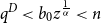


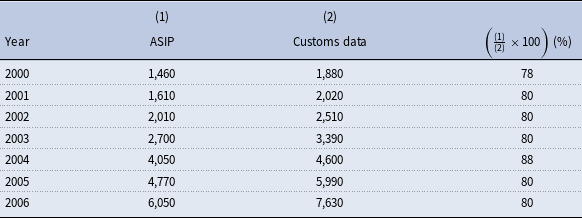
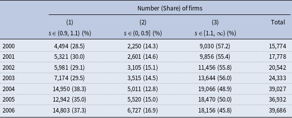
 s
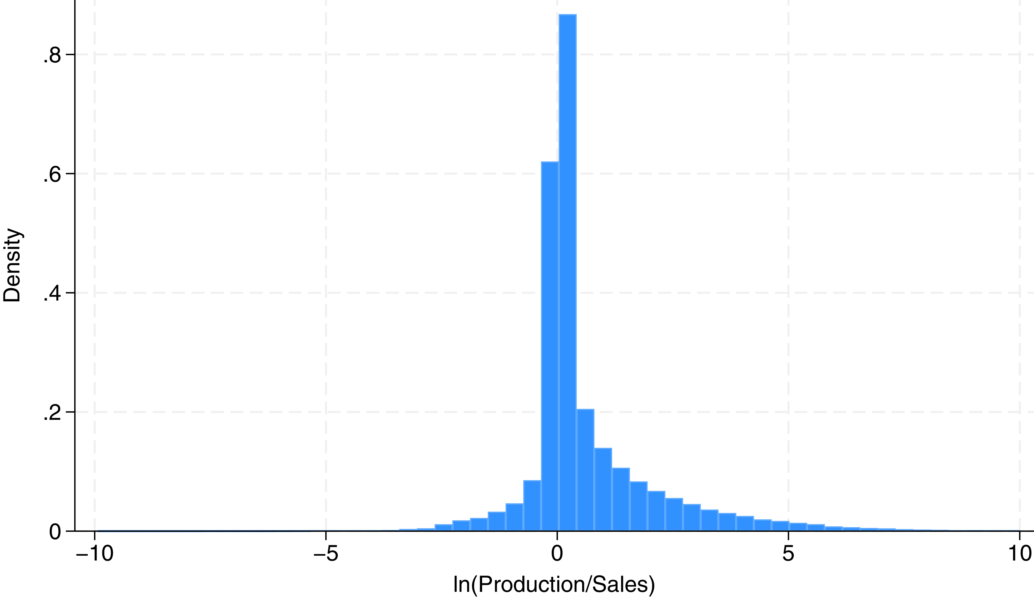
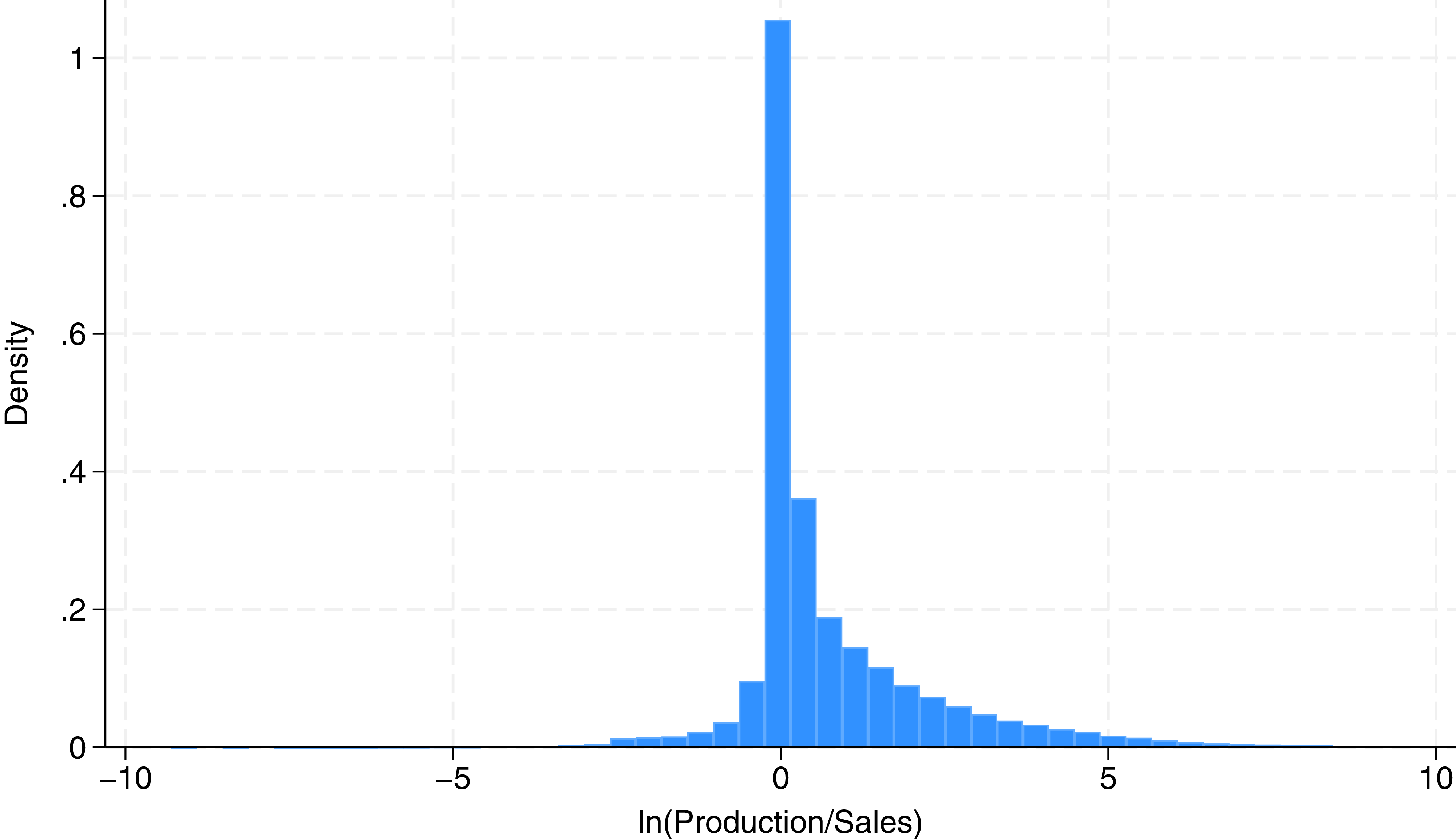
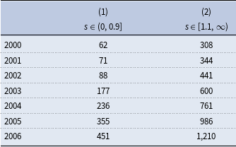
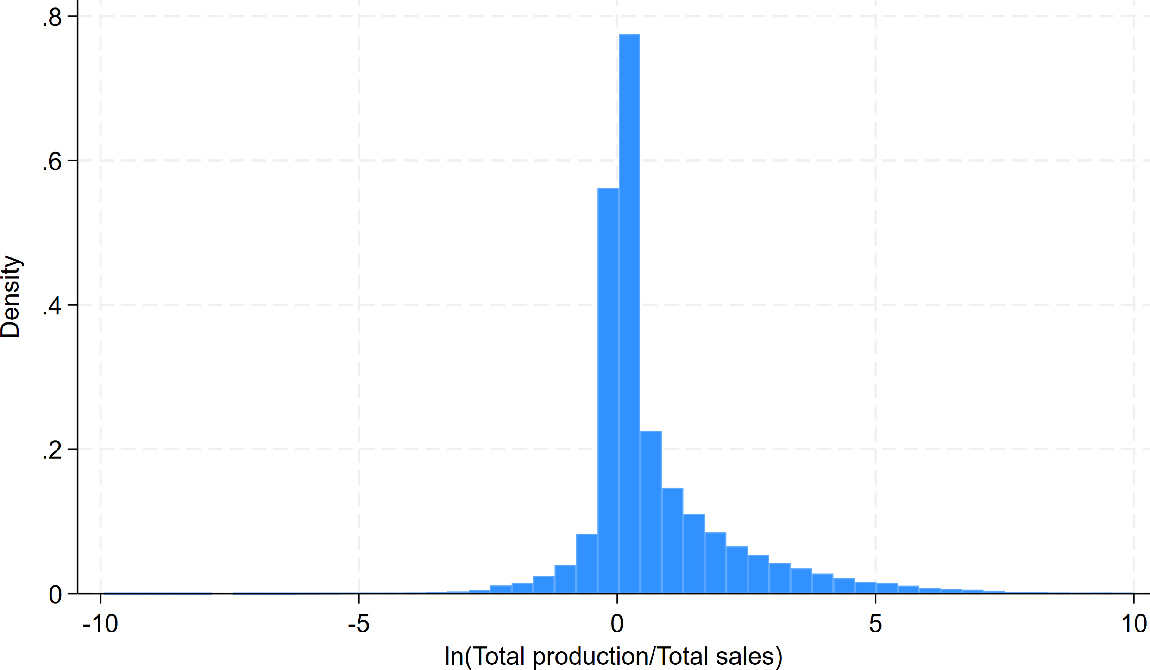
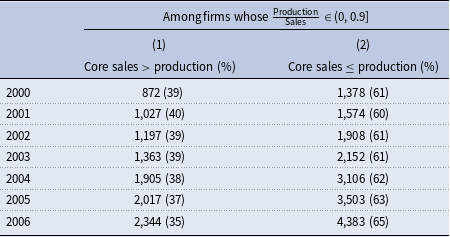
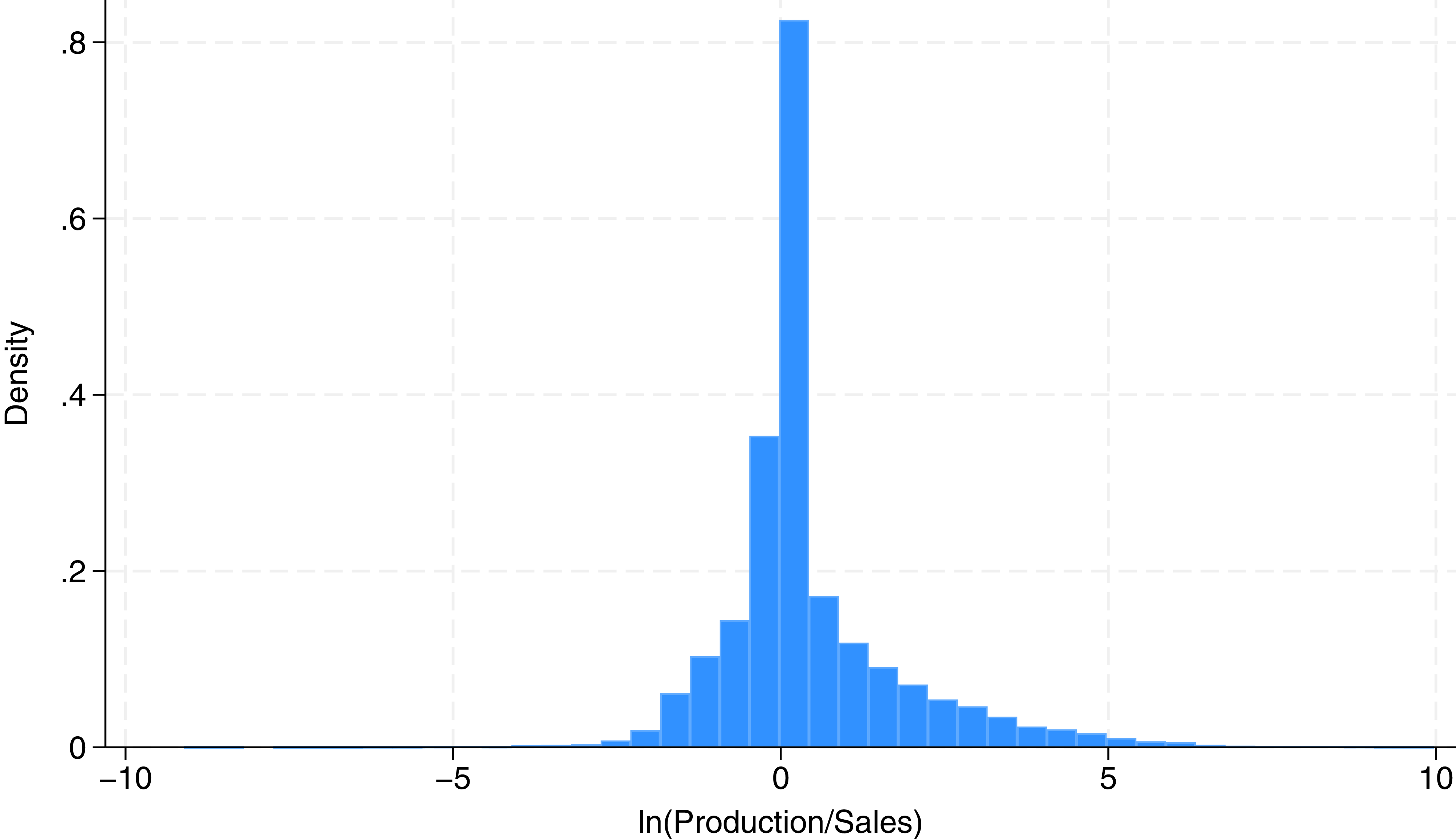
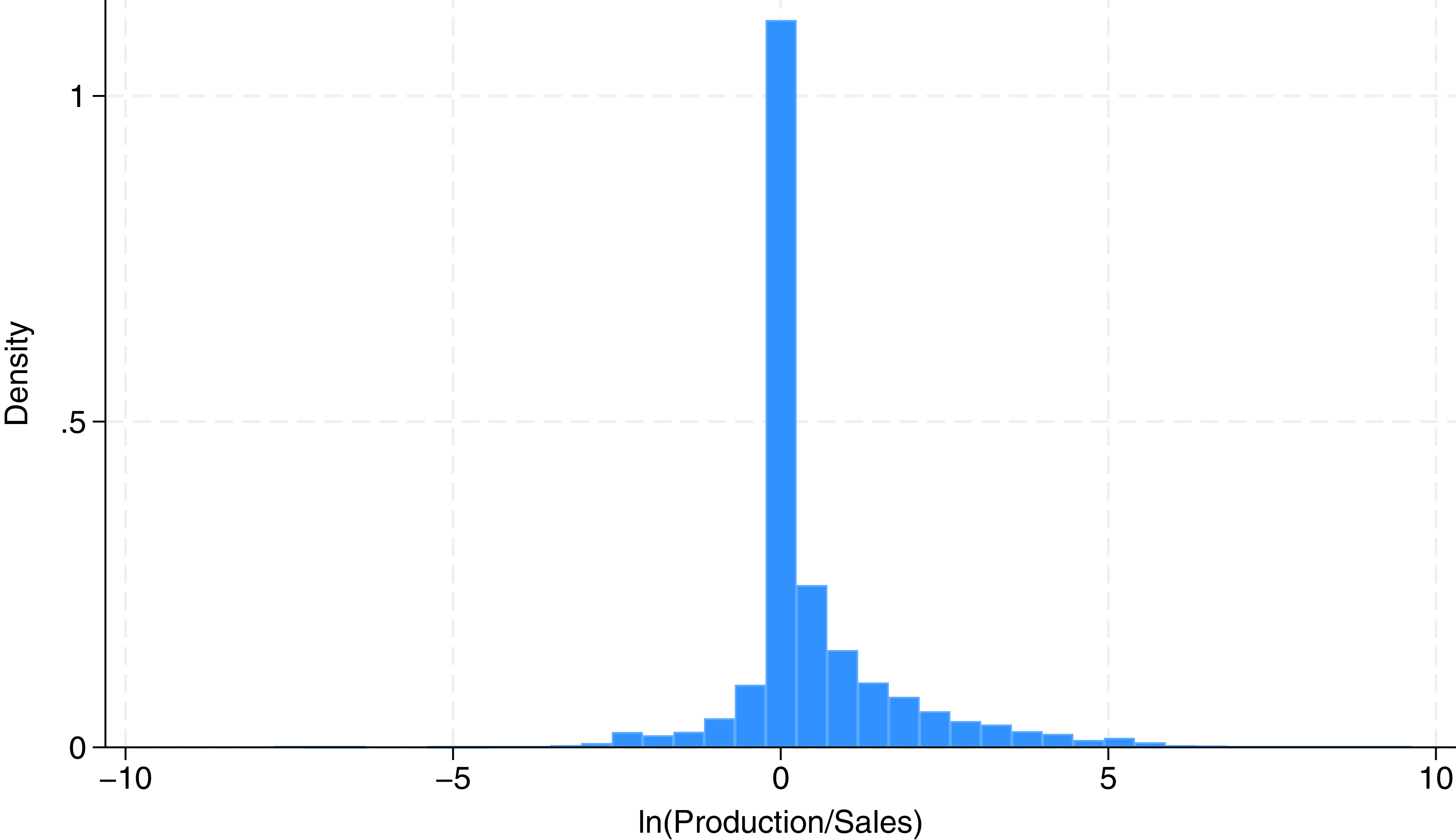
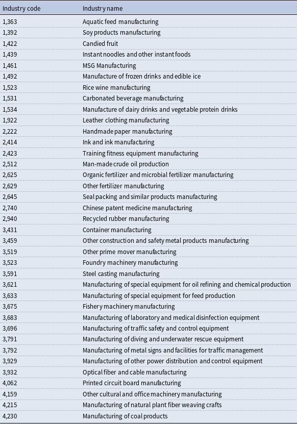
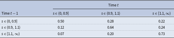
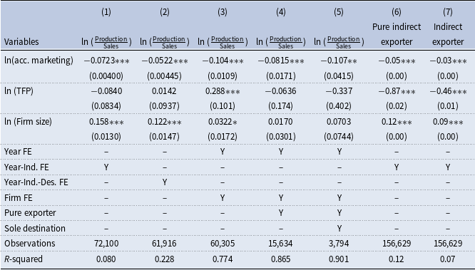
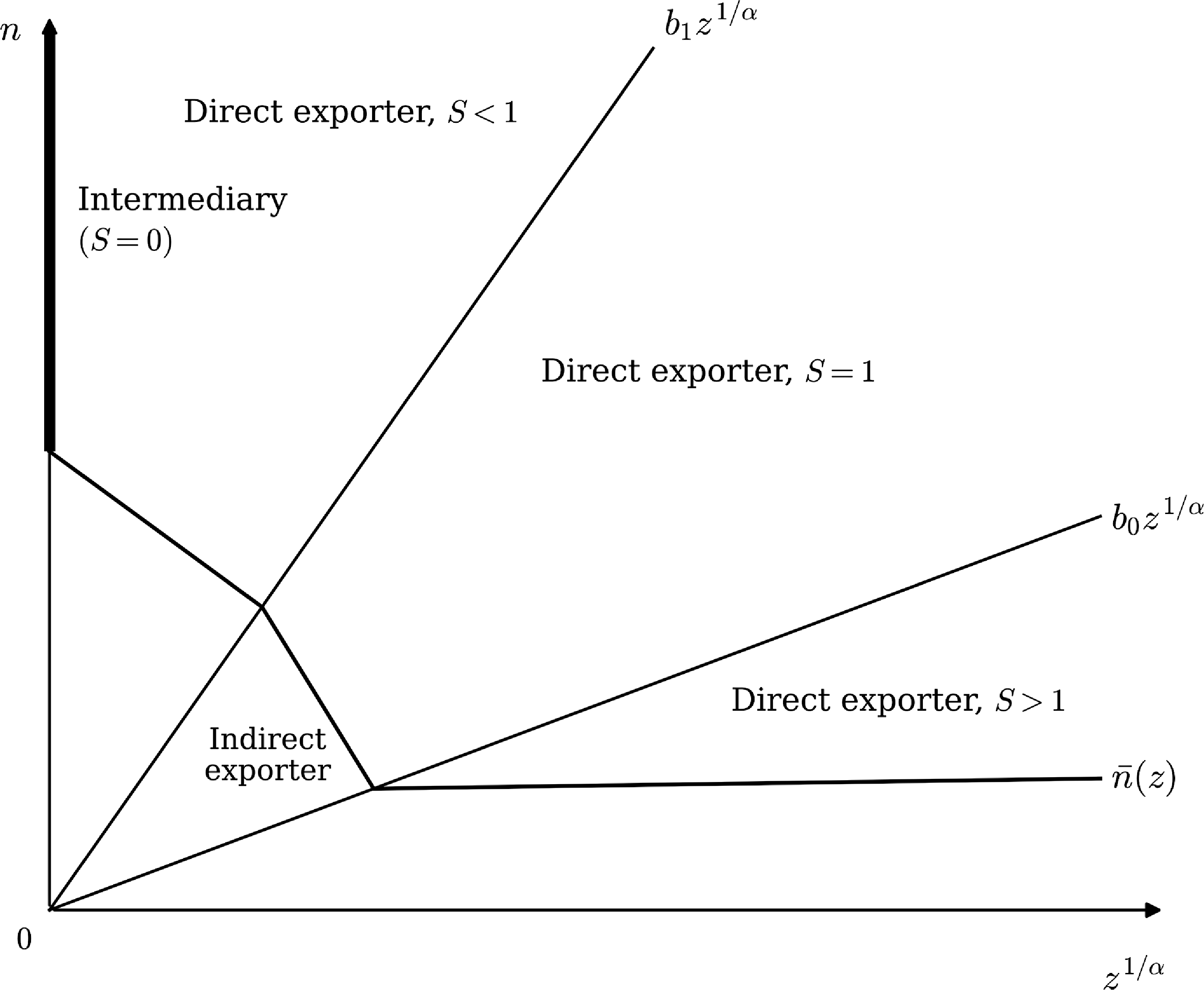
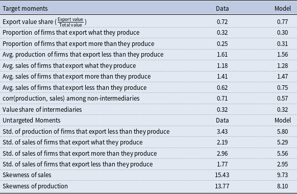

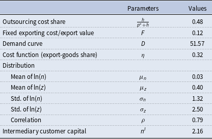

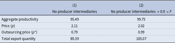

 Open access

