

Introduction
On any given day, fire stations don't know exactly how many firefighters will be needed, power plant operators don't know exactly what the demand for power will be and banks don't know exactly how much liquid capital they should have in reserve. In such systems, formally known as threshold systems, when demand exceeds capacity, the consequences can be dire – such as unchecked fires, power outages or short selling non-liquid assets to acquire emergency capital (for each of the above examples, respectively). To avoid this, managers of such systems need to create safety margins by setting the capacities of their systems near the upper end of the distribution of possible demand. That leads to underutilized capacity most of the time (e.g., idle firefighters, wasted power-generation capacity and underinvested assets), but prevents system failures caused by spikes in demand.
Another way to make a system more robust is to allow its components to pool resources to a greater degree. For example, firefighters may be allowed to call in reinforcements from neighboring precincts, failing or failed power plants might be allowed to shift demand to neighboring plants or banks might insure each other or share a common capital reserve.
We call such a modification pooling the system. In pooled systems, small failures are less damaging because pooling reduces the impact of failures of a system's most vulnerable components. However, a side effect of introducing pooling is increasing the coupling of system components (cf. Perrow, Reference Perrow1999). In particular, when one component fails, that imposes an additional cost on the other components, which strains their capacity and may cause further failures. This cascade of failures can continue until all components in the coupled system are no longer working. As a result, coupled systems can be susceptible to rare but large cascading failures in which a chain reaction of failures brings down the entire system. Simulations and analytic results have shown that a small amount of coupling is often enough to convert what would have been a small failure into a large chain of failures (Granovetter, Reference Granovetter1978; Watts, Reference Watts2002; Dobson et al., Reference Dobson, Carreras and Newman2005; Nedic et al., Reference Nedic, Dobson, Kirschen, Carreras and Lynch2006).
What makes pooled systems dangerous is that they create a decision environment where the risks involved are largely hidden from system operators, undermining their ability to accurately gauge the extent to which reducing capacity threatens the system. Pooled systems hide risks because they tend to produce initial records of operation in which few failures occur. That can motivate operators to cut costs by reducing safety margins. For example, managers might reduce the capacities of components of an electrical system or financial regulators might reduce capital reserve requirements for banks. Such changes can increase the probability of large cascading failures.
Furthermore, the benefits of increased pooling are highly visible (e.g., less wasted capacity and reduced frequency or impact of small failures, depending on the specific instantiation of the pooling). In contrast, the cost of increased pooling (increased risk of large failures as safety margins are reduced) is typically invisible – at least until a large failure occurs (by which point it's too late).
Highly pooled systems have another dangerous feature: since the likelihood of failure of each node is conditionally dependent upon the failure of other nodes in the system, the system as a whole can shift rapidly from no failures to total failure. There is good reason to believe that people do not recognize non-linearity in these sorts of systems and therefore can exhibit preferences that lead to catastrophic failures.
Indeed, people's ability to reason about non-linear systems is systematically flawed (e.g., De Bock et al., Reference De Bock, Van Dooren, Janssens and Verschaffel2002; Van Dooren et al., Reference Van Dooren, De Bock, Depaepe, Janssens and Verschaffel2003; Zhao, Reference Zhao2016). People tend to assume that systems are linear, and adjusting away from this assumption is effortful, requiring both numeracy skills and available working memory capacity (Thomson & Oppenheimer, Reference Thomson and Oppenheimer2016). As the deviation from linearity is even more extreme in coupled threshold systems than more commonly studied non-linear systems (such as those involving exponential or quadratic dependencies), there is ample reason to believe that people will struggle to make accurate judgments in such systems.
In sum, theory predicts that coupled threshold systems will be difficult to safely manage because they involve: (1) a hidden risk of cascading failure; and (2) a highly non-linear dependence of failure probability on size of safety margin. Given this, there is surprisingly little empirical research demonstrating failures in managing such systems or investigating how to prevent such failures.
This is troubling because coupled threshold systems are highly prevalent in domains as diverse as finance, infrastructure, health care, emergency response and engineering. Moreover, political and market forces can accentuate the danger. When one simultaneously increases pooling in a threshold system and reduces its safety margins, one reduces resource wastage due to unused capacity. One also reduces the frequency of small system failures. The net effect is to reduce the (short-term) cost of operating the system while increasing its apparent reliability. So politicians and firms have significant incentive to increase pooling and reduce safety margins (Boin et al., Reference Boin and Hart2003, p. 546; Elga, Reference Elga2012).
One might hope that existing regulations and procedures would compensate for the above incentives to prevent cascading failures. But in fact, cascading failures contributed to the 2003 Northeast blackout (affecting 15 million customers) (Perrow, Reference Perrow2007, pp. 211–213), the 1996 Western US blackout (affecting 7.5 million customers), the 1984 Western US blackout (affecting 3 million customers) (Hines et al., Reference Hines, Balasubramaniam and Sanchez2009, p. 26), a number of fires such as the 2007 and 2014 San Diego wildfires and the 2018 North Bay wildfires (Lagos et al., Reference Lagos, Lewis and Pickoff-White2018) and a large range of financial panics and crises, including the 2008 financial crisis (Kindleberger & Aliber, Reference Kindleberger and Aliber2005; Brunnermeier, Reference Brunnermeier2009; Sachs, Reference Sachs2009; Gorton & Metrick, Reference Gorton and Metrick2010; Yellen, Reference Yellen2013).
In several studies, we investigated whether coupled threshold systems are indeed as dangerous as theory would predict. Participants played an experimental game in which they were placed into the role of a power company executive and asked to choose safety margins for either coupled or uncoupled systems. To foreshadow results: as predicted by the aforementioned theory, participants in the coupled system condition failed to provide adequate safety margins. As a result, participants in the coupled system condition performed worse than those in the uncoupled system condition.
Study 1
Participants
Forty-six participants were recruited through Amazon.com's Mechanical Turk platform (for a discussion on the validity of results from this platform, see Paolacci et al., Reference Paolacci, Chandler and Ipeirotis2010) and participated in the study for monetary compensation.
Design and procedure
Participants were placed in the role of a power company CEO and were tasked with determining how much power to produce in each of 10 cities with the aim of maximizing profits. The cost of producing power was $5 per megawatt hour, and power was sold at $7 per megawatt hour. Thus, every sold unit generated a $2 profit and every unsold unit generated a $5 loss. If demand exceeded supply, the power plant would ‘crash’, meaning that: (i) no income could be generated; (ii) all expenses (production of power) remained; and (iii) a $5000 penalty was applied (see Supplementary Online Materials and Methods for wording of instructions).
Half of the participants were randomly assigned to be in an independent-plants condition and were informed:
If you happen to underestimate demand in a particular city, and as a result the power distributor in that city crashes, your remaining functional power plants will be completely unaffected. Although you will not earn any income from cities where the power distributors have crashed, the remaining functional power plants will still provide power to their own cities, and you can potentially make enough profits in those other cities to offset some of the losses from failed power plants.
The remaining participants were assigned to a coupled-plants condition, and were informed:
If you happen to underestimate demand in a particular city, and as a result the power distributor in that city crashes, your remaining functioning power plants will pick up some of the unfilled demand. 20 percent of the demand from any crashed power plant will be reallocated to the functioning power plants from other cities (each of the functioning plants will take an equal share of that demand). This will increase the demand at all of your other plants, allowing you to sell power that would otherwise go unused – assuming those other plants have enough capacity to handle this increased demand. However if the functioning power plants do not have the capacity to handle the increased demand, they too will crash. In such a situation, the Coupling Distributor would then reallocate 20 percent of the demand from those (newly crashed) plants to the remaining functioning plants. This process will continue until no additional functioning plants crash from the added load.
Participants in both conditions were given a fictional backstory to increase their motivation and interest in the game (see Supplementary Online Materials and Methods for wording).
Participants were then given a comprehension quiz testing their understanding of the setup and the within-game compensation scheme consisting of questions such as: “If you create 1000 megawatt hours of power, and the demand is 200 megawatt hours, how much money will you gain or lose?” If participants missed a question, they were required to reread the experimental directions until they achieved a perfect score on the quiz.
At the start of each trial, participants were shown their current cumulative cash balance (starting at $150,000), a reminder of the cost of producing power and an array of pictures representing 10 power plants (see Figure 1 for screenshot). Cumulative cash balances were allowed to go negative.
Section of a screenshot from Study 1. Participants set safety margins for 10 individual power plants after being informed of the expected demand.

An expected demand distribution was randomly generated for each city such that the midpoint of each city's demand distribution was independently sampled from a normal distribution with a mean of 1600 megawatt hours and a standard deviation of 100 megawatt hours. Each city was labeled with the expected demand range, which participants had been informed represented the width of a roughly bell-shaped distribution for power demand in that city.
Participants entered into text boxes the amount of power that they wished to produce in each city. Actual demand was then determined based on the distributions that participants had been provided. In the independent-plants condition, if a plant's power supply was at least as great as its city's demand, then the plant succeeded and supplied that amount of power. Otherwise, the plant failed and supplied no power.
Each participant's simulation was entirely independent from those of other participants. Thus, each participant faced a series of single-person decision problems, and (multi-person) game-theoretic considerations such as free-riding or collective optimality played no role.
In the coupled-plants condition, plant failures were determined by the following algorithm:
1. Set each plant's available capacity to the amount selected by the participant.
2. Set each plant's load to equal the power demanded by its associated city.
3. Any plant whose load exceeds its available capacity fails and supplies no power.
4. Twenty percent of the total demand from cities associated with newly failed plants is divided equally among unfailed plants, adding to their load.
5. Steps 3 and 4 are repeated until no additional plants fail.
A results screen then showed overall income and expenses for that day, the actual demand for power in each city, and whether the power plant in each city could supply all of the power that was asked of it. In the coupled-demand condition, power plant failures were animated, allowing participants to see when failures of some power plants caused further failures.
Participants completed 15 trials. After trials 2, 5, 8, 11 and 13, participants were shown snippets of storyline text intended to increase their engagement in the game.
Results
The data for five participants were excluded from the analysis: one participant due to a computer recording error, two for providing invalid input and two for failing to complete the study.
Participants in the coupled condition fared much worse than those in the independent condition. Participants in the independent condition earned an average total of $262,454, while participants in the coupled condition lost an average of $69,865 (t(40) = 2.241, p = 0.031).Footnote 1
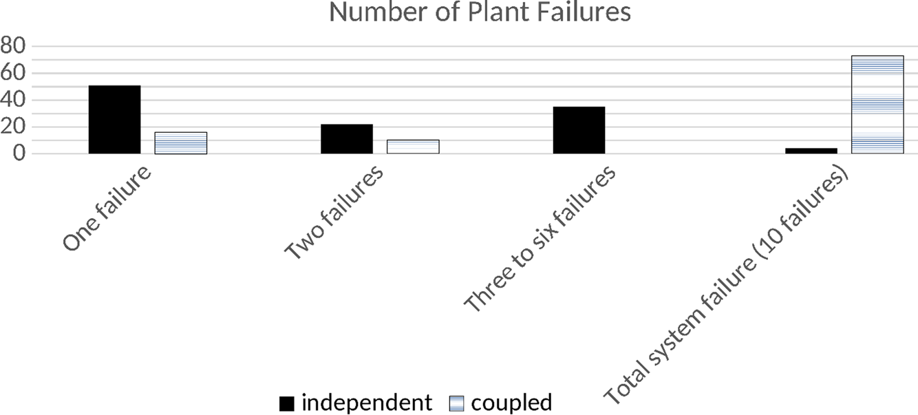
Part of the reason for this is that participants had fewer plants fail on average in the independent condition (x = 0.91) than in the coupled condition (x = 2.1), although this difference did not reach conventional levels of significance (t(40) = 1.9, p = 0.064). Importantly, total system failure happened 73 times in the coupled conditions, but only twice in the independent condition (χ 2(1, n = 75) = 67.21, p < 0.001). In contrast, mid-range failures (i.e., three to six failures) happened 34 times in the independent condition, but never in the coupled condition (see Figure 2).
Distribution of plant failures by condition. In the independent condition, participants observed small failures with some regularity, but almost never had total system failure. In contrast in the coupled condition, participants had few small failures, but were much more likely to see total system failure. There were no instances of seven to nine failures in either condition.

Discussion
One reason participants performed better in the independent condition was that, in that condition, they experienced isolated failures; single-plant failures were more than three times as likely in the independent condition as in the coupled condition. These small failures may have acted as early ‘danger signals’, leading participants to adopt more conservative safety margins – a safer strategy. In contrast, participants in the coupled condition, in the absence of isolated failures to indicate that risk was increasing, lowered safety margins (to increase profits) until the entire system crashed. Total system failures were more than 35 times as likely to occur in the coupled than independent condition.
Introducing coupling into a system changes the probability distribution of outcomes. In particular, it can make moderately bad outcomes (low-impact minor failures) less likely while making extremely bad outcomes (high-impact total system failures) more likely. Whether such a tradeoff is reasonable for a participant depends on the details of his or her risk preferences. In particular, it depends how much the participant values small but significant risks of large losses. So it is possible that participants earned less money in the coupled condition not because of error (as outlined in the introduction), but rather because their true risk preferences in the coupled condition favored choices with lower expected monetary values.
To test for this possibility, Study 2 was designed so that a third of the participants were given live previews of the expected distribution of plant failures across their possible choices, a third were given live previews of the expected profits (and losses) across their possible choices (cf. Sterman et al., Reference Sterman, Fiddaman, Frankck, Jones, McCauley, Rice, Sawin and Siegel2013) and a third were provided with no distribution information (as in Study 1). If in Study 1 participants were correctly assessing the risk profiles produced by their choices, then it would be expected that informing participants about those risk profiles would make little difference to their performance. On the other hand, if participants in the cascading condition were systematically underestimating the risks of large failures, then informing them of those risks would be expected to improve their performance.
Study 2
Participants
Three-hundred and seven participants were recruited through Amazon.com's Mechanical Turk platform and participated in the study for monetary compensation.
Design and procedure
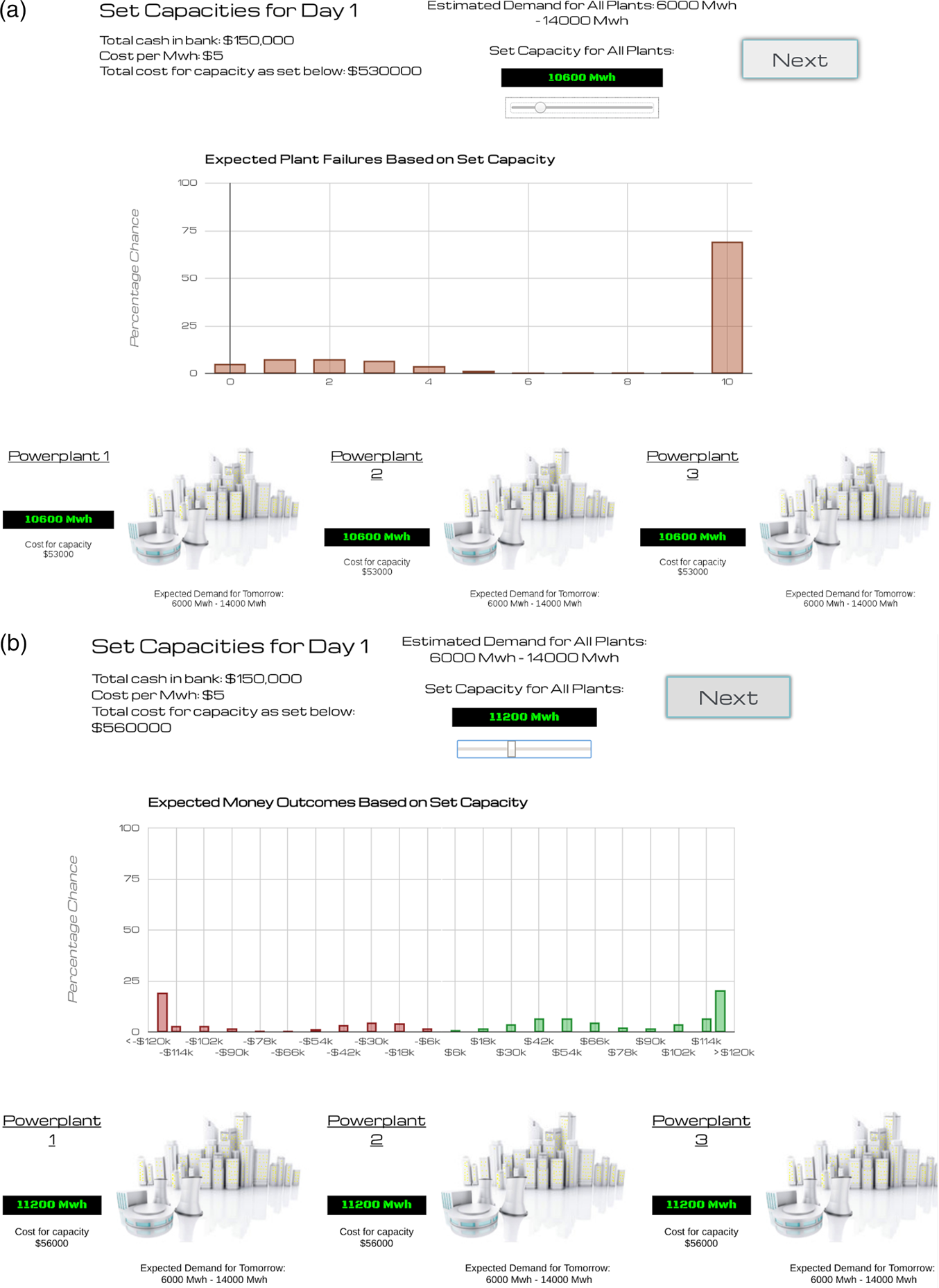
Study 2 closely mimicked the design of Study 1, with two main differences: (1) a third of the participants were given live previews of the expected distribution of plant failures across their possible choices, a third were given live previews of the expected profits (and losses) across their possible choices and a third were provided with no distribution information (as in Study 1; see Figure 3 for screenshots of the different conditions); and (2) to allow for real-time feedback, participants were asked to choose a single capacity level to be applied to all power plants on a given game day (trial).
(a) Screenshot from the Study 2 failure feedback condition. Participants chose safety margins for all power plants using an onscreen slider. As the slider was moved, participants could see a live-updating probability mass function for the expected number of plant failures for the currently selected safety margin. (b) Screenshot from the Study 2 money feedback condition. Participants chose safety margins for all power plants using an onscreen slider. As the slider was moved, participants could see a live-updating histogram showing the probability mass function for expected monetary outcomes for the currently selected safety margin.

Participants were randomly assigned to a condition in a 2 (independent vs. coupled) × 3 (no graph vs. failure graph vs. money graph) design. Each subject completed 10 trials. For simplicity, on each trial, each city's power demand was drawn from the same normal distribution with a standard deviation of 1000. To ensure that participants continued to respond to expected demand ranges, the mean of the distribution for power demand changed between trials, varying between 8000 and 12,000.
Capacity was set by moving an onscreen slider to positions that represented different levels of power generation. As participants in failure graph conditions moved the slider, they were shown a histogram representing the probability distribution for the number of expected plant failures given the currently selected capacity. Participants in money graph conditions were shown a histogram representing the probability distribution for expected net profits (or losses). Participants in no graph conditions were not given any distributional information, and thus were forced to determine the likely outcome themselves (as in Study 1). Participants in graph conditions were given explanations in advance of how to read the graphs (see Supplementary Online Materials and Methods for exact wording).
The algorithm for determining plant failures was the same as Study 1 except that in coupled conditions, 12% rather than 20% of the total unfilled demand from failed plants was reallocated. This compensated for the fact that, in a given trial, the expected demands between cities were more highly correlated in Study 2 than in Study 1, since in each Study 2 trial every city's demand was drawn from the same distribution. The overall result was that the algorithm in Study 2 produced cascades that were qualitatively similar to those in Study 1. Nevertheless, because of the parameter value change, Study 2 included a replication of the cascading vs. independent comparison from Study 1 using the new parameter value.
No motivational snippets were displayed between rounds.
Results
Five participants were removed for failing to complete the experiment. An additional five participants were removed as outliers for having a rate of failure falling at least eight standard deviations from the mean (these participants did not understand how to move the slider to change capacity).
As an absolute benchmark for performance in the game, we used Monte-Carlo sampling to estimate the strategy for each condition that maximized expected total monetary gain. In particular, for each game situation and approximate choice of power capacity, we averaged the monetary returns in 107 sample runs to estimate the expected return produced by that choice. This allowed us to estimate the choice for each game situation that maximized expected gain. We summed those gains to estimate the maximum possible expected gain for each experimental condition. For the independent condition, the maximal expected gain was approximately $829,000. For the coupled condition, it was approximately $830,000. These estimates also apply to Study 3 below.
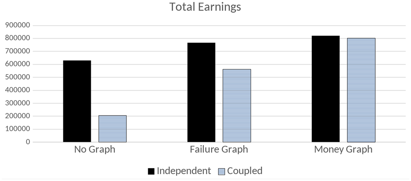
Replicating the findings from Study 1, participants performed significantly better in the independent condition than the coupled condition. This was the case even though a player who maximized expected gain would do at least as well in the coupled condition as he or she would in the independent condition. Within the no graph condition, participants in the coupled condition earned less over the course of the 10 trials (x = $205,968) than participants in the independent condition (x = $628,962), and this difference was statistically significant (t(96) = 3.6, p < 0.01). Although participants across the board performed better in the failure graph condition, participants still earned less in the coupled condition (x = $563,323) than in the independent condition (x = $766,134), and this difference was also statistically reliable (t(97) = 2.1, p < 0.05). Participants performed even better in the money graph condition, and here the significant difference between the independent condition (x = $819,886) and the coupled condition (x = $802,155) disappeared (t(97) = 0.21, p > 0.8). Notably, monetary gains in both money graph conditions were near optimal – within 4% of gains achieved by optimal play.
To make sense of this pattern, we ran a 2 (coupling level: coupled vs. independent) × 3 (graph type: no graph vs. failure-graph vs. money-graph) analysis of variance (ANOVA). There was a significant main effect for graph type (F(2,291) = 15.6, p < 0.001) and a main effect of coupling level (F(1, 291) = 13.7, p < 0.001), and these main effects were qualified by a graph type × coupling level interaction (F(2, 291) = 4.1, p < 0.05) (see Figure 4).
Average of total earnings (losses) in the independent vs. coupled conditions across the three graph conditions (no graph, failure graph and money graph) in Study 2. In the no graph condition, participants earned significantly more in the independent than coupled condition. When participants received failure graphs, their performance improved overall, but the discrepancy between the coupled and independent conditions decreased. In the money graph condition, the difference between coupled and independent conditions disappeared.

This difference in performance by condition appeared to once again be driven by the number of plant failures. In the no-graph condition, participants had more failures per trial in the coupled condition (x = 1.24) than in the independent condition (x = 0.81), and this difference was statistically significant (t(96) = 2.3, p < 0.05). In the failure graph condition, participants also had more failures in the coupled condition (x = 0.79) than in the independent condition (x = 0.51), which was marginally significant (t(96) = 1.7, p = 0.092). In the money graph condition, participants had similar numbers of failures in the coupled (x = 0.45) and in the independent (x = 0.49) conditions (t(96) = 0.30, p > 0.7). Unsurprisingly given this pattern, when we ran a 2 (coupling level: coupled vs. independent) × 3 (graph type: no graph vs. failure graph vs. money graph) ANOVA, we found a main effect for coupling (F(1,291) = 5.5, p < 0.05) and a main effect for graph type (F(2,291) = 12.0, p < 0.001), although the interaction was not statistically reliable (F(2,291) = 2.1, p = 0.12). Indeed, participants' allocation policies looked remarkably similar in both of the money graph conditions, suggesting that the failures in the coupled condition were due to a cognitive error in determining the risks of coupled systems, rather than a true reflection of participants' risk preferences.
Raw anonymized experimental data associated with this paper are publicly available at https://osf.io/wtpx5.
Discussion
Once again, participants had considerably worse outcomes in coupled than independent systems. However, when participants were given distributions of the possible outcomes of a given allocation policy, this performance deficit disappeared. This suggests that participants struggle to recognize the dangers of cascades in coupled systems when setting allocation policies; when they are alerted to the risks of having too-small safety margins, participants increase capacity and reduce the frequency of cascading failures.
The first two studies were not incentive compatible: participants earned fictional dollars, but success and failure in the context of the game had no real-world consequences. Thus, it is possible that participants were not sufficiently motivated to take the task seriously and optimize their outcomes. Moreover, the individual trials were not independent, which raises the possibility of strategic game play. Indeed, having a catastrophic failure in earlier trials may actually encourage people to play in riskier ways. After experiencing one catastrophic failure, there is not much downside to adopting an extremely risky policy – as one is going to go bankrupt anyway, additional failures have limited downside, but one might get lucky and pull oneself out of debt. While to some degree this is a feature that mimics real-world environments, it limits the inferential power of the preliminary studies by reducing the number of independent observations of the phenomenon, and it may lead to inflated estimates of the prevalence of catastrophic failure.
To rectify these shortcomings, a third study mimicked the ‘no-graph’ condition of Study 2 while adding an incentive-compatible compensation scheme.
Study 3
Participants
One-hundred and nineteen participants were recruited through Amazon.com's Mechanical Turk platform and participated in the study for monetary compensation.
Design and procedure
Study 3 game play proceeded as in the independent no graph and coupled no graph conditions from Study 2, except that an incentive-compatible compensation scheme was introduced. The backstory of the game was changed to make the ‘days’ within the game independent, and no cumulative balances were reported. Participants began the game with $10. One of 10 trials was randomly selected and participants gained or lost 1 cent for every 1000 game dollars that they gained or lost in that trial. Overall compensation was bounded so that participants could not earn less than $3 or more than $17. Participants were informed in advance of the compensation scheme.
Results
One participant dropped out of the study after the first simulated day, but since each trial was an independent observation, we were able to include that participant's partial data in the analyses. Removing that data point does not qualitatively affect the results.
Study 3 replicated our previous findings. Participants in the independent condition earned an average of $42,203 (in game money) per trial, while those in the coupled condition lost an average of $21,715 (in game money) per trial. A generalized linear mixed model with trial as a within-subject variable and condition as a between-subject variable showed this difference to be statistically reliable (F(1,1181) = 6.3, p < 0.05). This difference was driven by the number of plant failures, with participants in the coupled condition experiencing, on average, nearly twice as many failures (x = 1.7) as those in the independent condition (x = 0.83). As with earnings, a generalized linear mixed model with trial as a within-subject variable and condition as a between-subject variable revealed this difference to be statistically reliable (F(1,1181) = 274.7, p < 0.001).
Breaking down those failures, in the coupled condition there were 82 trials in which total system failure occurred (roughly 14% of trials), while in the independent condition total system failure never happened (χ 2(1, n = 82) = 82, p < 0.001). In contrast, mid-range failures (i.e., three to six failures) happened 65 times in the independent condition (roughly 11% of trials), but only 14 times in the coupled condition (roughly 2.5% of trials; χ 2(1, n = 79) = 32.9, p < 0.001).
There was also evidence that participants learned how to better manage coupled systems over the course of the experiment. While the correlation between trial number and earnings was not statistically reliable in the independent condition (r = 0.298, p > 0.05), that relationship in the coupled condition was significantly positive (r = 0.841, p < 0.01). These differences were driven by reductions in the number of plant failures over the course of the experiment.
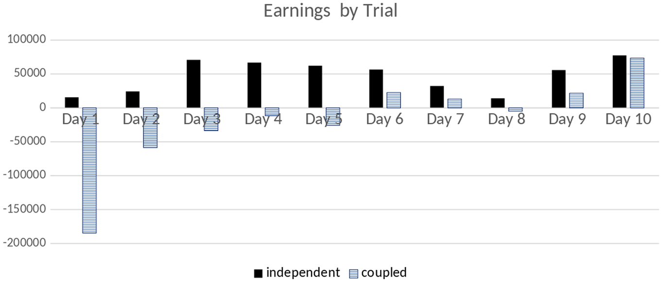
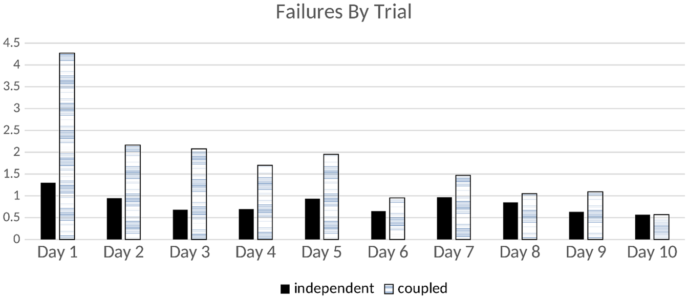
To put this in perspective, on Trial 1, participants in the coupled condition suffered an average of 4.3 failures and lost $184,748 (in game money), while those in the independent condition suffered an average of 1.3 failures and earned $15,235 (in game money; ttrial_1_failures(117) = 4.37, p < 0.001; ttrial_1_earnings(117) = 4.468, p < 0.001). However, by Trial 10, participants in the coupled condition suffered an average of only 0.569 failures and earned an average of $73,467 (in game money), while those in the independent condition suffered an average of 0.567 failures and earned an average of $77,080 (in game money; ttrial_10_failures(116) = 0.008, p > 0.99; ttrial_10_earnings(116) = 0.18, p > 0.85) (see Figures 5 and 6).Footnote 2
Earnings by trial in the independent and coupled conditions for Study 3. Participants in both conditions showed improvement over the course of the experiment, but this improvement was much greater in the coupled condition. In Trial 1, participants in the coupled condition performed significantly worse than those in the independent condition. By Trial 10, this difference had disappeared.

Failures by trial in the independent and coupled conditions for Study 3. While participants in the coupled condition suffered many more failures on Trial 1 than those in the independent condition, this difference had disappeared by Trial 10.

Discussion
As in Study 2, even though an optimal player would perform at least as well in the coupled condition as in the independent condition, in fact participants performed significantly worse in coupled than independent conditions. Even when trials are independent and performance is rewarded in an incentive-compatible manner, participants initially set buffers too low, leading to catastrophic failures. While participants appear to eventually learn how to appropriately manage a coupled system, that learning comes at the expense of massive failure that would have significant deleterious effects in real-world environments.
General discussion
Over three studies, our investigations highlighted a distinct hidden danger of pooled systems. Study 1 provided an initial demonstration that participants struggle to set appropriate capacity in pooled systems, and as a consequence have considerably worse outcomes. Study 2 replicated the findings of Study 1, further demonstrating that these findings are due to error rather than a reflection of participants' true risk preferences. Study 3 replicated these findings in an incentive-compatible framework and demonstrated that people learn how to avoid the dangers of coupled systems with experience, providing convergent evidence that underperformance in coupled systems is not a reflection of true risk preferences.
Taken together, these studies show that pooled systems have a hidden risk. While such systems are appealing on the surface because they reduce waste and the frequency of small failures, they also obscure the likelihood of catastrophic failure. Pooled systems are perilous because decision-makers get misleading information and feedback that is not optimized for how humans reason. While people can learn how to appropriately manage pooled systems given sufficient experience, that experience comes in the form of highly costly catastrophic failures.
Caveats
In the studies, a number of parameters of the system were set arbitrarily. These include the payoff for each unit of demand met, the cost of each unit of unused/wasted capacity, the penalty associated with the failure of a node (i.e., a power plant crashing) and the number of nodes in the system. It is important to note that while this is an existence proof of the dangers of coupled threshold systems, it does not mean that all pooled systems will necessarily lead to cascading, catastrophic failure. Future research will need to identify the boundary conditions and determine if there exist pooled systems that don't have the dangerous characteristics identified here.
Policy advice
There are two major viable policy responses to the challenges we have identified with pooled threshold systems: (1) increasing safety margins; and (2) reducing pooling.
Increasing safety margins
Pooling resources in threshold systems is actually helpful in reducing waste and increasing robustness so long as safety margins are sufficiently large. However, as the benefits of reducing safety margins are immediately obvious (less waste and consequently greater short-term profit) while the drawbacks are hidden (increased risk of catastrophic failure in the long term), there are strong pressures to reduce those margins to dangerous levels. Policies that encourage increased safety margins would therefore substantially mitigate the risk of pooling threshold systems.
In a seminal chapter, Thaler et al. (Reference Thaler, Sunstein, Balz and Shafir2013) lay out a set of principles for effective choice architecture, which apply to overcoming the challenges inherent in setting appropriate capacities for pooled systems. We use this framework to organize recommendations for policy-makers on how to reduce the risk of the negative impact of coupled systems.
Give feedback
One reason that highly pooled systems are so dangerous is that decision-makers receive feedback that the system is working, right up until the moment of catastrophic failure. Feedback systems need to be revised to inform policy-makers not just as to whether the system is robust in a current cycle, but also what would have happened with slightly greater pressure on the system. It may also be important to have decoupled feedback, even when the system itself is coupled. That is, even though the system as a whole is doing well, policy-makers should be informed when nodes would have failed had the coupling not been present (as seeing that some nodes would have failed may encourage more conservative allocation policies).
Understanding mappings
One challenge with coupled threshold systems is that decision-makers cannot easily calculate the likelihood of catastrophic outcomes for different capacity levels. Because risk in these systems increases in a non-linear manner, which is notoriously difficult for humans to understand (cf. Olsson et al., Reference Olsson, Enkvist and Juslin2006), there is not a clear mapping from choice to welfare. In Study 2, we provided decision-makers with information on how different levels of capacity relate to the likelihood of failures (including system-wide failures) and distributions of overall earnings, to great effect. However, Study 2 also shows that the specific nature of the mapping is important – information about the likely number of failures was less effective than information about likely financial outcomes. This underscores the importance of making sure the mappings are appropriately calibrated to the decision strategies that policy-makers are using.
Incentives
Explicitly incentivizing a larger safety margin (e.g., by subsidizing the system to reimburse the costs of unused/wasted capacity) may be able to reduce the danger of coupled threshold systems. More standard incentive schemes, such as the one used in Study 3, highlight the advantages of reducing buffers – notably, it is immediately obvious to the decision-maker that there is excess capacity and that money could be saved (in the short run) by reducing capacity. Of course, such risky strategies are penalized in the long run in the form of catastrophic failure. But myopia prevents decision-makers from taking account of those long-term consequences, which means that typical incentive schemes encourage dangerously low safety margins. An incentive scheme that explicitly rewards the maintenance of larger safety margins could offset the tendency to adopt risky strategies.
Of course, such reward structures could create perverse incentives toward waste. An organization that is paid for generating excess capacity might be inclined to generate more excess capacity than necessary. Therefore, it is important to be mindful of undesirable motivational effects when implementing such an incentive scheme.
Expect error
Knowing that decision-makers tend to reduce safety margins to dangerous levels, it may be worthwhile to design systems that are more robust to such errors. For example, to the extent that it is possible in a particular domain, it might be helpful to create a metaphorical (or literal) circuit breaker. The aim is that once a certain number of nodes in the system have failed, the breaker mechanism would disengage the remainder of the system before the entire system crashes. In the power grid case, this might involve a load-shedding scheme in which failing power components are deactivated without redirecting demand to their neighbors when the system as a whole is in a vulnerable state. While this sometimes produces local power shortages, it reduces the risk of total system failure (Perrow, Reference Perrow2007, pp. 215–220; Hines et al., Reference Hines, Balasubramaniam and Sanchez2009, pp. 25–26; Wei et al., Reference Wei, Lu, Tang and Lu2018). More generally, the idea is to construct systems so that when the decision-maker sets safety margins too low there is a failsafe in place.
Defaults
While our specific studies cannot speak to the effectiveness of default choices in encouraging decision-makers to maintain more responsible buffers, there is a large literature demonstrating that people often stick with a default (e.g., Dinner et al., Reference Dinner, Johnson, Goldstein and Liu2011). Certainly, it seems unlikely that a default choice of a high safety margin would discourage high safety margins, so to the extent that it might help, there seems only upside potential of such an intervention. One difficulty that arises when attempting to adopt this approach is identifying the appropriate default, as whoever is setting the default would likely be subject to the same challenges in identifying appropriate choices as the person setting safety margin policy. Still, there may be fewer pressures/incentives toward reducing capacity for the person setting the default, which might help somewhat overcome the biases observed in this paper.
Structuring complex choices
The final element of Thaler et al.'s (Reference Thaler, Sunstein, Balz and Shafir2013) framework seems less relevant to the present issue, as in our study the choice options were already well structured (see screenshots); the challenge wasn't the complexity of choices, but the failure to understand the consequences of those choices. However, it may be the case that in some coupled threshold systems the choices are not structured effectively, which might only exacerbate the problem.
Across all of the nudges based on Thaler et al.'s (Reference Thaler, Sunstein, Balz and Shafir2013) framework described above, the specifics will vary by context. While the deep structural problem of cascading failures is evidenced across most coupled threshold systems, there are obviously differences in the logistics of implementing policy in power systems as opposed to financial systems or first-response systems.
While we have described a nudge-based set of interventions above, another option is to mandate high safety margins, such as is often done with banks and capital reserve. Such mandates have costs: they can be politically difficult to implement, could require resources to enforce and may limit flexibility and creativity in managing systems. However, in some pooled systems, the consequences of catastrophic failure may be great enough to outweigh those costs.
Another sort of policy intervention is to limit the degree to which the system in question pools its resources and hence to reduce the degree to which its components are coupled. This might be implemented by encouraging or enforcing limits on the resources that a failing component can draw from other components. It might also be implemented by partitioning the system into zones and allowing pooling only within each zone.
The appropriate limits to pooling in a given case depend on the relative importance of increased safety and increased efficiency. As a result, no domain-neutral guidelines apply. But it is worth noting that one result seems to be fairly robust across models: when the coupling in a system is below a critical value, cascades of failures tend to die out quickly. When the coupling exceeds that value, however, cascades tend to continue until a large fraction of the units have failed (cf., Dobson, Reference Dobson2007). While it will typically not be feasible to effectively calculate the critical level of coupling for a large real-world system, policy-makers should keep in mind that there is a great gain in safety when the level of coupling is sub-critical.
Conclusions
Increasing interconnectivity and globalization has led to a rapid rise in coupled threshold systems across many domains. In addition to the finance, infrastructure and emergency response examples described above, these systems are prevalent in health care (e.g., whether or not pharmacies and hospitals stock sufficient medications for rare but highly contagious conditions), flood control (e.g., whether or not municipalities maintain sufficient levees and floodplains), food supply planning (e.g., how much crop diversity is required to achieve a prudent level of food security) and hybrid systems in which failures in one domain put stresses on another (e.g., disease outbreaks or terrorist attacks that simultaneously stress medical resources, physical infrastructure and financial systems) (Sheppard, Reference Sheppard2014). A better understanding of our cognitive deficits in managing coupled threshold systems and empirically tested interventions to improve such management could prevent catastrophic system failure in a number of important domains.
Acknowledgments
A. Elga gratefully acknowledges support from a 2014–2015 Deutshe Bank Membership at the Princeton Institute for Advanced Studies, the David A. Gardner ’69 Magic Project (through Princeton University's Humanities Council) and the Princeton Institute for International and Regional Studies (PIIRS) Research Community on Systemic Risk. The authors wish to acknowledge R.A. Taimur Ahmed, programmers Helen Colby and Paul Feitzinger, the Opp Lab, helpful discussions with David Clark Sanjeev Kulkarni, Ron Mandle, Don Mango, Nina Mazar, Ida Momennejad, George O'Brien, Nicole Oppenheimer, Emily Pronin, Luis Rayo, Eldar Shafir, Gene Stein, Savitar Sundaresan, Nassim Taleb and Jiaying Zap and audiences at the Casualty Actuaries of the Mid-Atlantic Region Conference, Cognitive Group of the University of California Los Angeles Psychology Department, Corridor Reading Group, Harvard Law School, International Conference on Thinking, Princeton Social Psychology Research Seminar, University of Pennsylvania and World Bank. Special thanks are owed to Daniel Cloud for conversations that provided the initial inspiration for the project.
Supplementary Material
To view supplementary material for this article, please visit https://doi.org/10.1017/bpp.2018.38.