1. INTRODUCTION
In the last two decades, integrated navigation has become a useful tool in determining the position and attitude of mobile sensors, in which information can be provided by Global Navigation Satellite Systems (GNSS), Inertial Navigation Systems (INS) and/or vision-based sensors. When this information is obtained directly by means of measurements from sensors on board the vehicle the term “direct geo-referencing” is used (Skaloud, Reference Skaloud1999). The integration of this data is usually done using a type of Kalman filter algorithm (Kalman, Reference Kalman1960). In the literature, the Kalman filter is derived as either a Best Predictor (BP) or a Best Linear Predictor (BLP) solution (Kalman, Reference Kalman1960; Gelb, Reference Gelb1974. P.107; Sanso, Reference Sanso and Sunkel1986; Teunissen and Khodabandeh, Reference Teunissen and Khodabandeh2013). The Minimum Mean Squared Error (MMSE) is the criterion used to select the best predictor or estimator. Up to now, one of the common solutions to this problem has been the traditional Extended Kalman Filter (EKF) (Jazwinski, Reference Jazwinski1970) due to the nonlinearities of the dynamic model. This algorithm has been widely used to provide a sub-optimal (or approximate optimal) nonlinear prediction of the state vector by means of a linearization procedure using a first-order Taylor approximation, in particular when the navigation systems have relied mainly on GNSS receivers as the primary source of position information for a vehicle. GNSS is able to provide precise positioning information to an unlimited number of users anywhere on the planet. However, a comprehensive study, referred to as the Volpe report (Volpe, Reference Volpe2001), indicates several vulnerabilities of GNSS associated with signal disruptions. GNSS provides precise information only under ideal conditions, that is, it normally requires an open environment.
Nevertheless, motivated by the new advances in remote sensor solutions in combination with traditional navigation sensors, some new systems have been proposed based on fusing remote sensing measurements with Global Positioning System (GPS)-INS measurements to achieve comprehensive, fast and real-time systems (Sheta, Reference Sheta2012). The linearized observation equations and/or system equations of these newly developed systems are referred to as Dynamic Errors-In-Variables (DEIV) models (Mahboub et al., Reference Mahboub, Saadatseresht and Ardalan2017a; Reference Mahboub, Saadatseresht and Ardalan2017b; Schaffrin and Iz, Reference Schaffrin and Iz2008). In such a case the classic EKF algorithm or its alternatives such as the Unscented Kalman Filter (UKF) (Julier and Uhlmann, Reference Julier and Uhlmann1997) may not be useful since they try to approximate the functional and stochastic model rather than properly modelling the dynamic environment.
Schaffrin and Iz (Reference Schaffrin and Iz2008) considered the observation equations of the DEIV model and proposed a Kalman filter algorithm named the Total Kalman Filter (TKF). Then Schaffrin and Uzun (Reference Schaffrin and Uzun2011) tried to impose a “data snooping” procedure on the TKF algorithm. As the characteristics of the noise of different sensors are often arbitrary and different, the structure of the noise supposed by Schaffrin and Iz (Reference Schaffrin and Iz2008) may not be useful. These algorithms and the techniques utilised are not ideally suited to the problem which is discussed in this paper. Therefore Mahboub et al. (Reference Mahboub, Saadatseresht and Ardalan2017a; Reference Mahboub, Saadatseresht and Ardalan2017b) presented a TKF algorithm with general weight matrices and named it the Weight Total Kalman Filter (WTKF).
In our problem the observation equations are generally nonlinear models and the system equations may be a DEIV model. Meanwhile, we want to impose a quadratic constraint. Even after linearization, the coefficient matrix of the linearized observation equations may remain noisy because of neglected random observed quantities such as errors derived from the control points. Thus in this paper we develop a Constrained Total Extended Kalman Filter (CTEKF) algorithm which can consider nonlinear dynamic models and quadratic constraints for integrated navigation.
Two points must be mentioned. Teunissen (Reference Teunissen1991) argued that by carefully iterating the EKF, one can solve the originally nonlinear formulation with the known rate of convergence of the Gauss-Newton method. See also Skoglund et al. (Reference Skoglund, Hendeby and Axehill2015) and Teunissen (Reference Teunissen1990). The second point is that Errors-In-Variables (EIV) models in their time invariant cases have been investigated by several valuable publications (for example, Amiri-Simkooei, Reference Amiri-Simkooei2017; Neitzel, Reference Neitzel2010; Snow, Reference Snow2012; Fang, Reference Fang2011; Reference Fang2014; Shen et al., Reference Shen, Li and Chen2011; Schaffrin, Reference Schaffrin2016; Schaffrin et al., Reference Schaffrin, Neitzel, Uzun and Mahboub2012; Schaffrin and Felus, Reference Schaffrin and Felus2008; Mahboub, Reference Mahboub2012; Reference Mahboub2014; Reference Mahboub2016; Mahboub et al., Reference Mahboub, Amiri-Simkooei and Sharifi2013; Reference Mahboub, Ardalan and Ebrahimzadeh2015; Mahboub and Sharifi, Reference Mahboub and Sharifi2013a; Reference Mahboub and Sharifi2013b; Paláncz and Awange, Reference Paláncz and Awange2012; Zhang et al., Reference Zhang, Tong and Zhang2013; Jazaeri et al., Reference Jazaeri, Schaffrin and Snow2014; Zeng et al., Reference Zeng, Liu and Yao2015).
This paper is organised as follows. In Section 2, a dynamic model of an integrated geo-referencing problem is defined. In Section 3, the CTEKF algorithm and its simplified form are developed, then, in Section 4, a case study gives insight into the efficiency of the algorithm proposed. Finally, in Section 5, we conclude the paper.
2. DYNAMIC MODEL OF INTEGRATED NAVIGATION
In recent years, integrated navigation techniques have started to be applied to mobile systems. They can provide a self-contained autonomous navigation solution and can be used as an alternative (or an addition) to traditional sensors (GNSS, INS and integrated GNSS/INS). Here we propose a new least squares prediction method called Constrained Total Extended Kalman Filter (CTEKF). The refined data from different sensors including GNSS, INS and remote sensors are fused using the newly developed Kalman filter algorithm in order to demonstrate the efficiency of the proposed method.
The dynamic model of an integrated direct geo-referencing problem in integrated navigation can be defined as follows (Sheta, Reference Sheta2012):
 $$\underline{y}_{i}=f_{i}\lpar \underline{x}_{i}\rpar +\underline{e}_{i} $$
 $$\underline{x}_{i}=\Phi_{i}x_{i-1}+g_{i}+\underline{u}_{i} $$
Equation (1) represents observation equations and Equation (2) are the system equations which are also called the dynamic model. This relates the unknown parameters at an epoch i to an earlier epoch i − 1. In the above equations  $\underline{y}_{i}$ is the m × 1 random observation vector,
 $\underline{e}_{i}$ is the m × 1 vector of observational noise, f i is a general non-linear function,
 $\underline{x}_{i}$ is the n × 1 random parameter vector (time dependent unknowns) which contains Three Dimensional (3D) position and attitude of the mobile sensors, that is,
 $\underline{x}_{i}=\left[\matrix{X_{i} & Y_{i} & Z_{i} &\omega_{i} & \varphi_{i} & \kappa_{i} }\right]$, Φi is the n × n transition matrix and
 $\underline{u}_{i}$ is the random system noise, g i is an independent time variable function and underlining (
 ) indicates random variables.
Equation (2) is usually produced by INS data and Equation (1) is usually provided by other sensors, for example, GPS and remote sensor data in an integrated navigation system. This arrangement can be changed according to the available sensors in a system. It is also assumed that the state vector is observed at an initial (previous) epoch:
 $$\underline{x}_{i-1}=x_{i-1}+\underline{e}_{i-1}^{0} $$
Here,  $\underline{e}_{i-1}^{0}$ is the random noise at the first epoch. Equations (1) to (3) usually represent the functional model of the dynamic problem. The corresponding stochastic model is defined as follows:
 $$\left[\matrix{ \underline{e}_{i} \cr \underline{u}_{i} \cr \underline{e}_{i-1}^{0} }\right]\sim \left(\left[\matrix{ 0 \cr 0 \cr 0 }\right]\comma \; \left[\matrix{ Q_{y_{i}} & 0 & 0 \cr 0 & \theta_{i} & 0 \cr 0 & 0 &\Sigma_{i-1}^{0} }\right]\right)$$
where  $Q_{y_{i}}$, θ i and
 $\Sigma_{i-1}^{0}$, are the corresponding dispersion matrices of the observation vector, the system equations and the observed unknown parameters at an initial epoch. Traditionally, the so called Extended Kalman Filter (EKF) is applied to solve the above problem; the first step requires the linearization of the functional model. In other words, the EKF algorithm is applied to the following linearized dynamic model by the assumption that
 $\underline{e}_{i}^{0}=0$:
 $$\underline{\delta y}_{i}=A_{i}\underline{\delta x}_{i}+\underline{e}_{i} $$
Here  $\underline{\delta y}_{i}$, A i and
 $\underline{\delta x}_{i}$ are given as follows:
 $$A_{i}=\left. {\partial f_{i} \over \partial \underline{x}_{i}} \right\vert _{\underline{x}_{i}=\underline{x}_{i}^{0}}\comma \; \quad \underline{\delta x}_{i}=\underline{x}_{i}-x_{i}^{0}\comma \; \quad \underline{\delta y}_{i}=\underline{y}_{i}-f_{i}\lpar \underline{x}_{i}^{0}\rpar $$
where  $x_{i}^{0}$ is the approximate value of the random parameter vector
 $\underline{x}_{i}$ which is as follows:
 $$x_{i}^{0}=\Phi_{i}\underline{x}_{i-1}+g_{i} $$
We can argue that the real dynamic model of the problem should be given by the following equations since some random observed quantities may still exist in A i which may be neglected. Moreover, if an INS is used to produce system equations, one encounters a DEIV model (Mahboub et al., Reference Mahboub, Saadatseresht and Ardalan2017a; Reference Mahboub, Saadatseresht and Ardalan2017b). Thus, we have:
 $$\underline{\delta y}_{i}=\lpar A_{i}-\underline{E}_{A_{i}} \rpar \underline{\delta x}_{i}+\underline{e}_{i} $$
 $$\underline{x}_{i}=\lpar \Phi_{i}-\underline{E}_{\Phi_{i}} \rpar x_{i-1}+g_{i}+\underline{u}_{i} $$
 $$\underline{x}_{i-1}=x_{i-1}+\underline{e}_{i-1}^{0} $$
In such a case, the EKF algorithm needs to be improved. The developed algorithm can be called a Total Extended Kalman Filter (TEKF) or a Constrained Total Extended Kalman Filter (CTEKF) algorithm after imposing the constraints. As we can see in the numerical example later in this paper, the TEKF algorithm is more accurate in solving integrated navigation problems. In the next section, the CTEKF algorithm and a simplified version are developed.
3. CONSTRAINED TOTAL EXTENDED KALMAN FILTER ALGORITHM
In this section, we develop the TEKF algorithm. For this, the dynamic model given by Equations (7) to (9) must be solved. Following Schaffrin and Iz (Reference Schaffrin and Iz2008) and Mahboub et al. (Reference Mahboub, Saadatseresht and Ardalan2017a; Reference Mahboub, Saadatseresht and Ardalan2017b), condition equations are used to solve this problem. Thus, Equations (8) to (10) should first be combined. From Equations (9) and (10) one has:
 $$\underline{x}_{i}=\lpar \Phi_{i}-\underline{E}_{\Phi_{i}} \rpar \lpar \underline{x}_{i-1}-\underline{e}_{i-1}^{0} \rpar +g_{i}+\underline{u}_{i} $$
Then Equation (11) can be linearized as follows:
 $$\matrix{ {{\underline{x} }_i} { \cong x_i^0 + {\left. {\displaystyle{{\partial {\underline{x} }_i} \over {\partial \underline{e}_{i - 1}^0 }}} \right\vert }_{\matrix{ {{\underline{E} }_{\Phi _i} = \underline{E} _{\Phi _i}^0 } \hfill \cr {{\underline{u} }_i = \underline{u} _i^0 } \hfill \cr {{\underline{e} }_{i - 1} = \underline{e} _{i - 1}^0 } \hfill \cr } }\lpar {x_{i - 1} - {\underline{x} }_{i - 1}} \rpar + {\left. {\displaystyle{{\partial {\underline{x} }_i} \over {\partial {\underline{u} }_i}}} \right\vert }_{\matrix{ {{\underline{E} }_{\Phi _i} = \underline{E} _{\Phi _i}^0 } \hfill \cr {{\underline{u} }_i = \underline{u} _i^0 } \hfill \cr {{\underline{e} }_{i - 1} = \underline{e} _{i - 1}^0 } \hfill \cr } }\lpar {{\underline{u} }_i - \underline{u}_i^0 } \rpar } \hfill \cr {} {\quad + {\left. {\displaystyle{{\partial {\underline{x} }_i} \over {\partial {\underline{E} }_{\Phi_i}}}} \right\vert }_{\matrix{ {{\underline{E} }_{\Phi _i} = \underline{E} _{\Phi _i}^0 } \hfill \cr {{\underline{u} }_i = \underline{u} _i^0 } \hfill \cr {{\underline{e} }_{i - 1} = \underline{e} _{i - 1}^0 } \hfill \cr } }vec\lpar {{\underline{E} }_{\Phi_i} - \underline{E}_{\Phi_i}^0 } \rpar } \hfill \cr {{\underline{x} }_i} { \cong x_i^0 + \lpar {\Phi_i} \rpar \lpar { - \underline{e}_{i - 1}^0 } \rpar + {\underline{u} }_i - \lpar {{\lpar {{\underline{x} }_{i - 1}} \rpar }^T \otimes I_n} \rpar {\underline{e} }_{\Phi _i}} \hfill \cr {{\underline {\delta x} }_i} { = {\underline{x} }_i - x_i^0 \cong - \Phi _i\underline{e} _{i - 1}^0 + {\underline{u} }_i - {\underline{E} }_{\Phi _i}{\underline{x} }_{i - 1}} \hfill \cr }$$
where the approximate value  $x_{i}^{0}$ for the unknown parameter vector
 ${\underline x}_{i}$ at an epoch i can be obtained as follows by the assumption that
 ${\underline E}_{\Phi_{i}}^{0} \cong 0_{n \times n}$,
 ${\underline e}_{i-1}^{0} \cong 0_{n\times 1}$ and
 $ {\underline u}_{i}^{0}\cong 0_{n\times 1}$:
 $$x_{i}^{0}=\Phi_{i}\underline{x}_{i-1}+g_{i} $$
If we insert Equation (12) into Equation (8) yields
 $$\underline{\delta y}_{i}=\lpar A_{i}-\underline{E}_{A_{i}} \rpar \lpar -\Phi_{i}\underline{e}_{i-1}^{0}+\underline{u}_{i}-\underline{E}_{\Phi_{i}}\underline{x}_{i-1} \rpar +\underline{e}_{i} $$
We also seek to impose a quadratic constraint and use a Quaternion approach to solve the singularity problems at the Euler (90°) angles. In such a case, a quadratic constraint can be considered during the integrated direct geo-referencing problem. This quadratic constraint can be shown as follows:
 $$\underline{x}_{i}^{T}C\underline{x}_{i}=c_{0} $$
Here C is a symmetric matrix and c 0 is a nonnegative scalar. Moreover, if we want to impose the constraint Equation (15) to the target function, it should be combined with Equation (11). In other words, Equations (15) and (11) give the following quadratic constraint:
 $$\lpar \lpar \Phi_{i}-\underline{E}_{\Phi_{i}} \rpar \lpar \underline{x}_{i-1}-\underline{e}_{i-1}^{0} \rpar +g_{i}+\underline{u}_{i} \rpar ^{T}C\lpar \lpar \Phi_{i}-\underline{E}_{\Phi_{i}} \rpar \lpar \underline{x}_{i-1}-\underline{e}_{i-1}^{0} \rpar +g_{i}+\underline{u}_{i} \rpar =c_{0} $$
It should be noted that we do not linearize the non-linear constraints. Due to Equations (14) and (16), the target function of the Constrained Extended Total Kalman Filter (CETKF) is given as follows:
 $$\eqalign{&\Phi\lpar \underline{e}_{i}\comma \; \underline{e}_{A_{i}}\comma \; \lambda_{i}\comma \; \underline{e}_{\Phi_{i}}\comma \; \underline{u}_{i}\comma \; \underline{e}_{i-1}^{0}\comma \; \mu_{i} \rpar =\underline{e}_{i}^{T}Q_{y_{i}}^{-1}\underline{e}_{i}+\underline{e}_{A_{i}}^{T}Q_{A_{i}}^{-1}\underline{e}_{A_{i}}+ \underline{u}_{i}^{T}\theta _{i}^{-1}\underline{u}_{i}+\underline{e}_{\Phi_{i}}^{T}Q_{\Phi _{i}}^{-1}\underline{e}_{\Phi_{i}}\cr &\quad +{\underline{e}^{0}_{i-1}}^{T}\lpar \Sigma_{i-1}^{0} \rpar ^{-1}\underline{e}_{i-1}^{0}+2\lambda_{i}^{T}\lpar \underline{\delta y}_{i}-\underline{e}_{i}-\lpar A_{i}-\underline{E}_{A_{i}} \rpar \lpar -\Phi_{i}\underline{e}_{i-1}^{0}+\underline{u}_{i}-\underline{E}_{\Phi_{i}}\underline{x}_{i-1} \rpar \rpar \cr &\quad +\mu_{i}\lpar \underline{b}_{i}^{T}C\underline{b}_{i}-c_{0} \rpar }$$
where μi and λi are the Lagrange multipliers of the quadratic constraint and  $\underline{b}_{i}$ is as follows:
 $$\underline{b}_{i}=\lpar \Phi_{i}-\underline{E}_{\Phi_{i}} \rpar \lpar \underline{x}_{i-1}-\underline{e}_{i-1}^{0} \rpar +g_{i}+\underline{u}_{i} $$
For optimisation, if tildas ( ) indicate predicted vectors and hats (
 ) denote estimated ones the following necessary conditions must hold:
 $$\left. {\partial \Phi \over \partial \tilde{e}_{i}} \right\vert \tilde{e}_{i}\comma \; \tilde{e}_{A_{i}}\comma \; \hat{\lambda }_{i}\comma \; \tilde{e}_{\Phi _{i}}\comma \; \tilde{u}_{i}\comma \; \tilde{e}_{i-1}^{0}\comma \; \hat{\mu }_{i}=2\lpar \tilde{e}_{i}^{T}Q_{y_{i}}^{-1}-\hat{\lambda }_{i}^{T}\rpar =0 $$
 $$\eqalign{ \left. {\displaystyle{{\partial \Phi } \over {\partial {\tilde e}_{A_i}}}} \right\vert {\tilde e}_i\comma \; {\tilde e}_{A_i}\comma \; {\hat \lambda }_i\comma \; {\tilde e}_{\Phi _i}\comma \; {\tilde u}_i\comma \; \tilde e_{i - 1}^0 \comma \; {\hat \mu }_i = & 2\hat \lambda _i^T \lpar {{\lpar { - \Phi_i\underline{e}_{i - 1}^0 + {\underline{u} }_i - {\underline{E} }_{\Phi_i}{\underline{x} }_{i - 1}} \rpar }^T \otimes I_m} \rpar \cr & + \hbox{2}\tilde e_{A_i}^T Q_{A_i}^{ - 1} = 0} $$
 $$\eqalign{ \left. {\displaystyle{{\partial \Phi } \over {\partial {\tilde e}_{\Phi_i}}}} \right\vert {\tilde e}_i\comma \; {\tilde e}_{A_i}\comma \; {\hat \lambda }_i\comma \; {\tilde e}_{\Phi _i}\comma \; {\tilde u}_i\comma \; \tilde e_{i - 1}^0 \comma \; {\hat \mu }_i = & 2\hat \lambda _i^T \lpar {{\lpar {{\underline{x} }_{i - 1}} \rpar }^T \otimes \lpar {A_i - {\tilde E}_{A_i}} \rpar } \rpar + 2\tilde e_{\Phi _i}^T Q_{\Phi _i}^{ - 1} \cr & - 2{\hat \mu }_i\underline{b} _i^T C\lpar {{\lpar {{\underline{x} }_{i - 1} - \tilde e_{i - 1}^0 } \rpar }^T \otimes I_n} \rpar = 0} $$
 $$\left. {\displaystyle{{\partial \Phi } \over {\partial {\tilde u}_i}}} \right\vert \tilde e_i\comma \; \tilde e_{A_i}\comma \; \hat \lambda _i\comma \; \tilde e_{\Phi _i}\comma \; \tilde u_i\comma \; \tilde e_{i - 1}^0 \comma \; \hat \mu _i = - 2\hat \lambda _i^T \lpar {A_i - {\tilde E}_{A_i}} \rpar + \hbox{2}\tilde u_i^T \theta _i^{ - 1} + 2\hat \mu _i\underline{b} _i^T C = 0 $$
 $$\eqalign{ \left. {\partial \Phi \over \partial \tilde{e}_{i-1}^{0}} \right\vert \tilde{e}_{i}\comma \; \tilde{e}_{A_{i}}\comma \; \hat{\lambda }_{i}\comma \; \tilde{e}_{\Phi _{i}}\comma \; \tilde{u}_{i}\comma \; \tilde{e}_{i-1}^{0}\comma \; \hat{\mu }_{i}= &2\hat{\lambda }_{i}^{T}\lpar A_{i}-\tilde{E}_{A_{i}} \rpar \lpar \Phi_{i} \rpar +2\tilde{e}{^{0}_{i-1}}^{T}\lpar \Sigma_{i-1}^{0} \rpar ^{-1}\cr & -2\hat{\mu }_{i}\underline{b}_{i}^{T}C\lpar \Phi_{i}-\tilde{E}_{\Phi_{i}} \rpar =0 } $$
 $$\eqalign{\left. {\displaystyle{{\partial \Phi } \over {\partial {\hat \lambda }_i}}} \right\vert {\tilde e}_i\comma \; {\tilde e}_{A_i}\comma \; {\hat \lambda }_i\comma \; {\tilde e}_{\Phi _i}\comma \; {\tilde u}_i\comma \; \tilde e_{i - 1}^0 \comma \; {\hat \mu }_i & = 2\lpar {\delta y_i - {\tilde e}_i - \lpar {A_i - {\underline{E} }_{A_i}} \rpar } \cr & \quad {\lpar { - \Phi_i\underline{e}_{i - 1}^0 + {\underline{u} }_i - {\underline{E} }_{\Phi_i}{\underline{x} }_{i - 1}} \rpar } \rpar ^T = 0} $$
 $$\left. {\displaystyle{{\partial \Phi } \over {\partial {\hat \mu }_i}}} \right\vert \tilde e_i\comma \; \tilde e_{A_i}\comma \; \hat \lambda _i\comma \; \tilde e_{\Phi _i}\comma \; \tilde u_i\comma \; \tilde e_{i - 1}^0 \comma \; \hat \mu _i = \underline{b} _i^T C\underline{b} _i - c_0 = 0 $$
 ${\tilde e}_i$ and
 ${\tilde e}_{A_{i}}$ can be obtained from Equations (19) and (20) as follows:
 $$\tilde{e}_{i}=Q_{y_{i}}\hat{\lambda }_{i} $$
 $$\tilde{e}_{A_{i}}=-Q_{A_{i}}\lpar \lpar -\Phi_{i}\tilde{e}_{i-1}^{0}-\tilde{E}_{\Phi_{i}}\underline{x}_{i-1}+\tilde{u}_{i} \rpar \otimes I_{m} \rpar \hat{\lambda }_{i}=-Q_{A_{i}}R_{i}^{1}\hat{\lambda }_{i} $$
Equations (21), (22) and (23) lead to:
 $$\eqalign{ {{\tilde e}_{\Phi _i}} \hfill & { = Q_{\Phi _i}\lpar {\lpar {\lpar { - {\underline{x} }_{i - 1}} \rpar \otimes {\lpar {A_i - {\tilde E}_{A_i}} \rpar }^T} \rpar {\hat \lambda }_i + \lpar {\lpar {{\underline{x} }_{i - 1} - \tilde e_{i - 1}^0 } \rpar \otimes I_n} \rpar C{\underline{b} }_i{\hat \mu }_i} \rpar } \hfill \cr {} \hfill & { = Q_{\Phi _i}\lpar {R_i^2 {\hat \lambda }_i + R_i^3 C{\underline{b} }_i{\hat \mu }_i} \rpar } \hfill \cr } $$
 $$\eqalign{& {{\tilde u}_i} = \theta _i\lpar {{\lpar {A_i - {\tilde E}_{A_i}}\rpar }^T{\hat \lambda }_i - C{\underline{b}}_i{\hat \mu }_i}\rpar \cr \hfill} $$
 $$\eqalign{ {\tilde e_{i - 1}^0 } \hfill & { = \Sigma _{i - 1}^0 \lpar { - {\lpar {\lpar {A_i - {\tilde E}_{A_i}} \rpar \lpar {\Phi_i} \rpar } \rpar }^T{\hat \lambda }_i + {\lpar {\Phi_i - {\tilde E}_{\Phi_i}} \rpar }^TC{\underline{b} }_i{\hat \mu }_i} \rpar } \hfill \cr {} \hfill & { = \Sigma _{i - 1}^0 \lpar {R_i^4 {\hat \lambda }_i + R_i^5 C{\underline{b} }_i{\hat \mu }_i} \rpar } \hfill \cr } $$
By inserting Equations (26) to (30) into Equation (24), the vector of Lagrange multipliers  $\hat{\lambda }_{i}$ can be estimated as follows:
 $$\eqalign{ & {\delta y_i - Q_{y_i}{\hat \lambda }_i - \lpar {A_i - {\tilde E}_{A_i}} \rpar \theta _i\lpar {{\lpar {A_i - {\tilde E}_{A_i}} \rpar }^T{\hat \lambda }_i - C{\underline{b} }_i{\hat \mu }_i} \rpar + \lpar {{\lpar {\Phi_i\tilde e_{i - 1}^0 } \rpar }^T \otimes I_m} \rpar Q_{A_i}R_i^1 {\hat \lambda }_i} \hfill \cr {} \hfill & {\quad - {\lpar {R_i^2 } \rpar }^TQ_{\Phi _i}\lpar {R_i^2 {\hat \lambda }_i + R_i^3 C{\underline{b} }_i{\hat \mu }_i} \rpar + \lpar {A_i} \rpar \Phi _i\Sigma _{i - 1}^0 \lpar {R_i^4 {\hat \lambda }_i + R_i^5 C{\underline{b} }_i{\hat \mu }_i} \rpar = 0 \to } \hfill \cr {} \hfill & {{\hat \lambda }_i = \lpar {Q_{y_i} + \lpar {A_i - {\tilde E}_{A_i}} \rpar \theta_i{\lpar {A_i - {\tilde E}_{A_i}} \rpar }^T + {\lpar {R_i^2 } \rpar }^TQ_{\Phi_i}R_i^2 - A_i\Phi_i\Sigma_{i - 1}^0 R_i^4 } } \hfill \cr {} \hfill & {\qquad - { {\lpar {{\lpar {\Phi_i\tilde e_{i - 1}^0 } \rpar }^T \otimes I_m} \rpar Q_{A_i}R_i^1 } \rpar }^{ - 1}\lpar {\delta y_i + \lpar {A_i - {\tilde E}_{A_i}} \rpar \theta_iC{\underline{b} }_i{\hat \mu }_i - {\lpar {R_i^2 } \rpar }^T} } \hfill \cr {} \hfill & {\qquad {{\rm }Q_{\Phi_i}R_i^3 C{\underline{b} }_i{\hat \mu }_i + A_i\Phi_i\Sigma_{i - 1}^0 R_i^5 C{\underline{b} }_i{\hat \mu }_i} \rpar } \hfill \cr } $$
The Lagrange multiplier μ̂i can be estimated by inserting Equations (26) to (30) into Equation (25) as follows:
 $$\eqalign{ & {\underline{b} _i^T C\lpar {\lpar {\Phi_i - {\tilde E}_{\Phi_i}} \rpar \lpar {{\underline{x} }_{i - 1} - \tilde e_{i - 1}^0 } \rpar + g_i + {\tilde u}_i} \rpar - c_0 = 0 \to \underline{b} _i^T C\Phi _i{\underline{x} }_{i - 1} - \underline{b} _i^T C{\tilde E}_{\Phi _i}{\underline{x} }_{i - 1}} \hfill \cr {} \hfill & {\quad - \underline{b} _i^T C\lpar {\Phi_i - {\tilde E}_{\Phi_i}} \rpar \tilde e_{i - 1}^0 + \underline{b} _i^T Cg_i + \underline{b} _i^T C{\tilde u}_i - c_0 = 0 \to } \hfill \cr {} \hfill & {{\hat \mu }_i = {\lpar {\underline{b}_i^T C\lpar {\lpar {{\lpar {{\underline{x} }_{i - 1}} \rpar }^T \otimes I_n} \rpar Q_{\Phi_i}R_i^3 + {\lpar {R_i^5 } \rpar }^T\Sigma_{i - 1}^0 R_i^5 + I_n} \rpar C{\underline{b} }_i} \rpar }^{ - 1}} \hfill \cr {} \hfill & {\qquad \lpar {\underline{b}_i^T C\lpar {\Phi_i{\underline{x} }_{i - 1} - \lpar {{\lpar {{\underline{x} }_{i - 1}} \rpar }^T \otimes I_n} \rpar Q_{\Phi_i}R_i^2 {\hat \lambda }_i - {\lpar {R_i^5 } \rpar }^T\Sigma_{i - 1}^0 R_i^4 {\hat \lambda }_i + g_i} } } \hfill \cr {} \hfill & {\qquad + { {\theta_i{\lpar {A_i - {\tilde E}_{A_i}} \rpar }^T{\hat \lambda }_i} \rpar - c_0{\rm }} \rpar } \hfill \cr } $$
Note that in Equation (32) the inverse of the matrix exists since it is a scalar quantity. After prediction of random observed variables  $\tilde{e}_{i}\comma \; \tilde{e}_{A_{i}}\comma \; \tilde{e}_{\Phi_{i}}\comma \; \tilde{u}_{i}$ and
 $\tilde{e}_{i-1}^{0}$ iteratively using Equations (26) to (30), we must update the measured unknown parameters
 $\underline{x}_{i-1}$ and the corresponding dispersion matrix for the next epoch i. According to Welch and Bishop (Reference Welch and Bishop2001), the updated dispersion matrix can be obtained by applying variance propagation rules. For this, we apply it to Equation (11). Then the updated dispersion matrix for the next epoch is given by
 $$D\lpar \underline{x}_{i} \rpar =K_{i}.blkdiag\lpar D\lpar \underline{x}_{i-1} \rpar \comma \; D\lpar e_{i-1}^{0} \rpar \!\comma \; D\!\lpar u_{i} \rpar \comma \; D\!\lpar E_{\Phi_{i}} \rpar \rpar {.K_{i}}^{T} $$
where the “blkdiag” operator constructs a block diagonal matrix from input arguments with
 $$\eqalign{K_{i}&=\left[\matrix{ {\partial \underline{x}_{i} \over \partial \underline{x}_{i-1}} & {\partial \underline{x}_{i} \over \partial e_{i-1}^{0}} &{\partial \underline{x}_{i} \over \partial u_{i}} & {\partial \underline{x}_{i} \over \partial E_{\Phi_{i}}}}\right]\cr &=\left[\matrix{ \lpar \Phi_{i}-\tilde{E}_{\Phi_{i}} \rpar & -\lpar \Phi_{i}-\tilde{E}_{\Phi_{i}} \rpar & I_{n} & -\lpar \lpar \underline{x}_{i-1}-\tilde{e}_{i-1}^{0} \rpar^{T}\otimes I_{n} \rpar }\right].}$$
Due to the nonlinearities contained within DEIV models, it is not deemed necessary to compute the rigorous variance matrix, although if required in practice, Equation (30) usually works well. To obtain the rigorous variance matrices one should apply the results of Teunissen (Reference Teunissen1989) and Grafarend and Awange (Reference Grafarend and Awange2012).
From Equation (12) the update of the unknown parameters  ${\tilde x}_i$ is obtained as follows:
 $$\eqalign{ \tilde{x}_{i}=\widetilde{\delta x}_{i}+x_{i}^{0} \qquad\qquad\cr \widetilde{\delta x}_{i}=-\Phi _{i}\tilde{e}_{i-1}^{0}+\tilde{u}_{i}-\tilde{E}_{\Phi _{i}}\underline{x}_{i-1}\cr x_{i}^{0}=\Phi_{i}\underline{x}_{i-1}+g_{i}\qquad\quad} $$
The prediction part is done by Equations (26) to (30) and the update part for the next epoch is given by Equations (30) and (34). Summarising, the proposed CETKF algorithm is given by the following:
Step 1:  $\underline{E}_{\Phi_{i}}^{0}\cong 0_{n\times n}$,
 $\underline{e}_{i-1}^{0}\cong 0_{n\times 1}$,;
 $\thinspace \hat{\mu }_{i}^{0}=0$,
 $x_{i}^{0}=\Phi_{i}\underline{x}_{i-1}+g_{i}$ and
 $\thinspace \underline{u}_{i}^{0}\cong 0_{n\times 1}$;
Step 2: for an epoch i ∈ N compute iteratively:
 $$\eqalign{\hat{\lambda }_{i} & =\lpar Q_{y_{i}}+\lpar A_{i}-\tilde{E}_{A_{i}} \rpar \theta_{i}\lpar A_{i}-\tilde{E}_{A_{i}} \rpar^{T}+\lpar R_{i}^{2} \rpar^{T}Q_{\Phi_{i}}R_{i}^{2}-A_{i}\Phi_{i}\Sigma_{i-1}^{0}R_{i}^{4} -\lpar \lpar \Phi_{i}\tilde{e}_{i-1}^{0} \rpar^{T}\otimes I_{m} \rpar Q_{A_{i}}R_{i}^{1} \rpar ^{-1} \cr & \quad \lpar {\delta y}_{i}+\lpar A_{i}-\tilde{E}_{A_{i}} \rpar \theta_{i}C\underline{b}_{i}\hat{\mu }_{i}-\lpar R_{i}^{2} \rpar^{T}Q_{\Phi_{i}}R_{i}^{3}C\underline{b}_{i}\hat{\mu }_{i}+A_{i}\Phi_{i}\Sigma_{i-1}^{0}R_{i}^{5}C\underline{b}_{i}\hat{\mu }_{i} \rpar \cr {\hat{\mu}}_{i} & =\lpar \underline{b}_{i}^{T}C\lpar \lpar \lpar \underline{x}_{i-1} \rpar^{T}\otimes I_{n} \rpar Q_{\Phi_{i}}R_{i}^{3}+\lpar R_{i}^{5} \rpar^{T}\Sigma_{i-1}^{0}R_{i}^{5}+I_{n} \rpar C\underline{b}_{i} \rpar ^{-1} \cr & \quad \lpar \underline{b}_{i}^{T}C\lpar \Phi_{i}\underline{x}_{i-1}-\lpar \lpar \underline{x}_{i-1} \rpar^{T}\otimes I_{n} \rpar Q_{\Phi_{i}}R_{i}^{2}\hat{\lambda }_{i}-\lpar R_{i}^{5} \rpar^{T}\Sigma_{i-1}^{0}R_{i}^{4}\hat{\lambda }_{i}+g_{i}+\theta_{i}\lpar A_{i}-\tilde{E}_{A_{i}} \rpar^{T}\hat{\lambda }_{i} \rpar -c_{0} \rpar \cr \tilde{e}_{i} & =Q_{y_{i}}\hat{\lambda }_{i} \cr \tilde{e}_{A_{i}} & =-Q_{A_{i}}\lpar \lpar -\Phi_{i}\tilde{e}_{i-1}^{0}-\tilde{E}_{\Phi_{i}}\underline{x}_{i-1}+\tilde{u}_{i} \rpar \otimes I_{m} \rpar \hat{\lambda }_{i}=-Q_{A_{i}}R_{i}^{1}\hat{\lambda }_{i} \cr \tilde{e}_{\Phi_{i}} & = Q_{\Phi_{i}}\lpar \lpar \lpar -\underline{x}_{i-1} \rpar \otimes \lpar A_{i}-\tilde{E}_{A_{i}} \rpar^{T} \rpar \hat{\lambda }_{i}+\lpar \lpar \underline{x}_{i-1}-\tilde{e}_{i-1}^{0} \rpar \otimes I_{n} \rpar C\underline{b}_{i}\hat{\mu }_{i} \rpar =Q_{\Phi_{i}}\lpar R_{i}^{2}\hat{\lambda }_{i}+R_{i}^{3}C\underline{b}_{i}\hat{\mu }_{i} \rpar \cr \tilde{u}_{i} & =\theta_{i}\lpar \lpar A_{i}-\tilde{E}_{A_{i}} \rpar^{T}\hat{\lambda }_{i}-C\underline{b}_{i}\hat{\mu }_{i} \rpar \cr \tilde{e}_{i-1}^{0} & =\Sigma_{i-1}^{0}\lpar -\lpar \lpar A_{i}-\tilde{E}_{A_{i}} \rpar \lpar \Phi_{i} \rpar \rpar^{T}\hat{\lambda }_{i}+\lpar \Phi_{i}-\tilde{E}_{\Phi_{i}} \rpar^{T}C\underline{b}_{i}\hat{\mu }_{i} \rpar =\Sigma_{i-1}^{0}\lpar R_{i}^{4}\hat{\lambda }_{i}+R_{i}^{5}C\underline{b}_{i}\hat{\mu }_{i} \rpar }$$
Step 3: after one sees the convergence at Step 2 for an epoch i, compute the state vector and its corresponding dispersion matrix at this epoch as follows:
 $$\eqalign{K_{i} & =\left[\matrix{ \lpar \Phi_{i}-\tilde{E}_{\Phi_{i}}\rpar & -\lpar \Phi_{i}-\tilde{E}_{\Phi_{i}} \rpar & I_{n} & -\lpar \lpar \underline{x}_{i-1}-\tilde{e}_{i-1}^{0} \rpar^{T}\otimes I_{n} \rpar }\right]\cr D\lpar \underline{x}_{i} \rpar & =K_{i}.blkdiag\lpar D\lpar \underline{x}_{i-1} \rpar \!\comma \; D\lpar e_{i-1}^{0} \rpar \!\comma \; D\!\lpar u_{i} \rpar \comma \; D\!\lpar E_{\Phi_{i}} \rpar \rpar {.K_{i}}^{T} \cr \tilde{x}_{i} & =\widetilde{\delta x}_{i}+x_{i}^{0} \cr \widetilde{\delta x}_{i} & =-\Phi _{i}\tilde{e}_{i-1}^{0}+\tilde{u}_{i}-\tilde{E}_{\Phi _{i}}\underline{x}_{i-1}}$$
Step 4: for the next epoch i + 1, put  $\underline{x}_{i}=\tilde{x}_{i}$,
 $\Sigma_{i}^{0}=Q_{x_{i}}$ and repeat the steps 1 to 3.
Note: if C = 0 and c 0 = 0, a simplified TEKF algorithm is obtained which may be useful for some problems.
4. SIMULATION AND A CASE STUDY
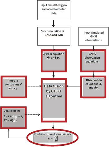
In this section, we numerically examine random neglected quantities that demonstrate, through simulation, that the EKF solution is less unsuitable than the CTEKF. Then, the CTEKF is applied to a case study. For the simulation, a simulated data set was used. The simulation was based on the block diagram as shown in Figure 1. In this example, a GNSS/Inertial Measurement Unit (IMU) system is considered. Two types of datasets were included for this test: a gyro and accelerometer dataset and a GNSS dataset, both obtained from different sources. More information may be found at www.Spirent.com.
Simulator block diagram.

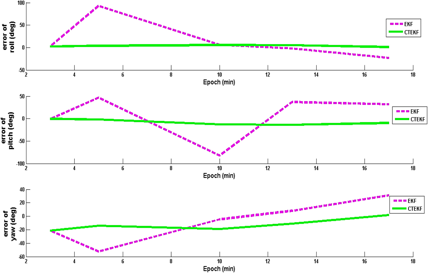
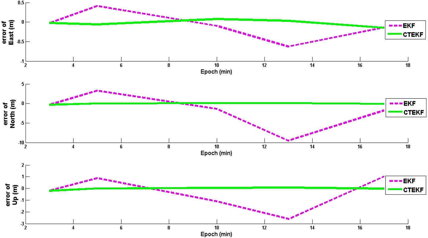
The observation equations and system equations are given by Equations (4), (8), (9) and (10). The time series of position prediction errors for the EKF and CTEKF algorithms are plotted in Figure 3 while the attitude (rotation) prediction errors are illustrated in Figure 2. In these figures, 3D position and 3D attitude are decomposed into three subplots so that each component can be assessed separately. East, North and Up are the three components of 3D position. 3D attitude of the mobile sensor is decomposed by Roll, Pitch and Yaw rotations. The navigation solution was improved as shown in Figures 2 and 3. The results demonstrate that the EKF algorithm is divergent since it could not model the random neglected noise which appeared in the coefficient matrices of the dynamic model.
Attitude (rotation) prediction error time series.

Position prediction error time series.

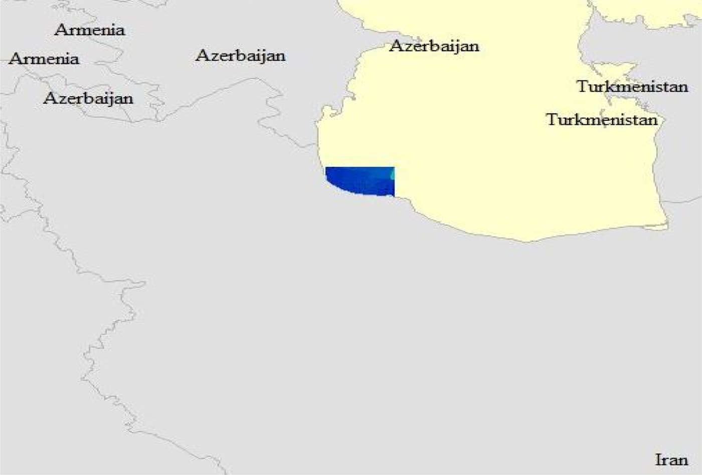
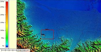
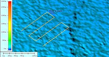
Next, we apply the proposed CTEKF algorithm to determine the position and attitude of a mobile sensor which has been moved in an area located in the Guilan province in the north of Iran. The trajectory is illustrated in Figures 4 to 6 We applied the CTEKF and EKF algorithms to the above example and compared the results with the post-processed solution as the true solution.
The location of the vision-based navigation case study.

The location of the vision-based navigation study on a Digital Elevation Model (DEM).

The trajectory of the mobile sensor on DEM.

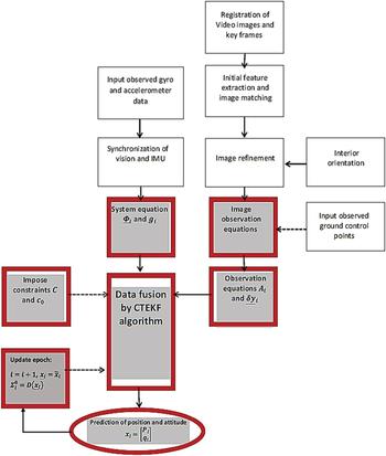
Here, we have to solve the integrated navigation for a vision/IMU system. In the block diagram shown in Figure 7, it can be seen how the data for this problem are prepared and then fused using the proposed Kalman filer. Three data sets are included in the test. They are gyro and accelerometer data, image data and ground points. A database of the geo-referenced satellite images of the area was built on the Speeded-Up Robust Features (SURF) algorithm in order to identify features within the dataset. The output contains descriptors for selected features that form the classes. Once a set of key points is detected in the real-time aerial images, they are matched with the set of SURF descriptors available in the database.
Vision/IMU navigation system block diagram.

Given conjugate correspondence points between the real-time images and the images from the database, the object-space transformation parameters can be estimated through the mathematical model of the collinearity. The vision aid for the Vision/IMU system uses the image matching position to update the INS error states using the Kalman filter algorithm. In other words, the collinearity equations are used to predict the position of the perspective centre of the camera through the concept of photogrammetric resection. The object space transformation parameters and the output of the photogrammetric resection are then used as the update for the INS Kalman filter for position updates. The camera and IMU specification are shown in Tables 1 and 2. In the rest of this section, we analytically examine how the vision system and IMU data produce the corresponding observation and system equations.
Error description of IMU data.

Camera specification.

If we want to produce the system equations from INS data, we have to consider Equation (9) as the system equations, and these are a set of differential equations. See Sheta (Reference Sheta2012) and Jekeli (Reference Jekeli2001) for more information. These equations describe the input gyroscope and accelerometer measurement input to the local frame mechanisation and the output curvilinear coordinates; three velocity components and three attitude components. The input to the computation process are the angular increments measured by the gyroscopes and the velocity increments measured by the accelerometers. The rotation matrix is updated by using Equation (9). The Quaternion approach is used in the update because it deals with the singularity problems of the Euler angles at a 90° angle. According to Sheta (Reference Sheta2012) we can argue that Equation (9) is set as follows:
 $$\underline{\Phi }_{i}=\left[\matrix{ I_{3} & 0 \cr 0 & I_{4}+\displaystyle{{1}\over{2}}\left[\matrix{ \underline{c} & \underline{d} &-\underline{b} & \underline{a} \cr -\underline{d} & \underline{c} &\underline{a} & \underline{b} \cr \underline{b} & -\underline{a} &\underline{c} & \underline{d} \cr -\underline{a} & -\underline{b} &-\underline{d} & \underline{c} } \right]}\right]$$
 $$g_{i}=\left[\matrix{ D_{i}\underline{V}_{i}{\Delta t}_{i} \cr 0 \cr }\right]$$
 $$x_{i}=\left[\matrix{ P_{i} \cr q_{i} \cr}\right]$$
where  $q_{i}^{T}=\left[\matrix{ q_{1} & q_{2} &q_{3} & q_{4} }\right]_{i}$,
 $\underline{V}_{i}$ is produced by the observed velocity increments, D i is a deterministic matrix depends on radius of curvature, Δ t i is time increments between two epochs and
 $P_{i}^{T}=\left[\matrix{ \varphi_{i} &\lambda_{i} & h_{i} }\right]$ or
 $P_{i}^{T}=\left[\matrix{ \hbox{X}_{i} &\hbox{Y}_{i} & Z_{i} }\right]$ in Cartesian coordinates. The noisy coefficients a, b, c and d are provided by the observed angular increments. The latitude φ, longitude λ and geodetic height h are the position components.
In some numerical examples, we see that considering a quadratic constraint may improve the solution. This situation can be seen when we want to impose the quadratic constraints of quaternion angles, for instance. In other words, if we want to use the quaternion angles q 1, q 2, q 3 and q 4, it is well-known that the following quadratic condition must hold:
 $$q_{1}^{2}+q_{2}^{2}+q_{3}^{2}+q_{4}^{2}=1 $$
In practice, when differential equations are used to describe the input gyroscope and accelerometer measurements input, one can apply Equation (38) to the integrated navigation problem. Then, the matrix C and the scalar c 0 in quadratic constraint given by Equation (15), can be determined by the following equations
 $$\left[\matrix{ P_{i}\cr q_{i} }\right]^{T}C\left[\matrix{ P_{i}\cr q_{i} }\right]=c_{0} $$
 $$q_{i}^{T}q_{i}=1 $$
 $$c = \left[{\matrix{ 0 & 0 & 0 & 0 & 0 & 0 & 0 \cr 0 & 0 & 0 & 0 & 0 & 0 & 0 \cr 0 & 0 & 0 & 0 & 0 & 0 & 0 \cr 0 & 0 & 0 & 1 & 0 & 0 & 0 \cr 0 & 0 & 0 & 0 & 1 & 0 & 0 \cr 0 & 0 & 0 & 0 & 0 & 1 & 0 \cr 0 & 0 & 0 & 0 & 0 & 0 & 1 \cr } } \right]\semicolon \; \quad c_0 = 1$$
The observation equations are usually produced from GNSS or remote sensed data or both. The non-linear function  $f_{i}\lpar \underline{x}_{i}\rpar $ can be provided depending on the type of sensor. In this example we used vision data and the corresponding equation is the well-known co-linearity condition. Also some ground noisy control points exist in this area. The observation equations can update the exterior orientation parameters using these points and the co-linearity condition. The observation equations for a pair of the vision data
 $x_{i}^{image}$ and
 $y_{i}^{image}$ is obtained as follows:
 $$x_{i}^{image}=x_{p}-f\displaystyle{{m_{11}\lpar X_{g}-X_{i} \rpar +m_{12}\lpar Y_{g}-Y_{i} \rpar +m_{13}\lpar Z_{g}-Z_{i} \rpar }\over{m_{31}\lpar X_{g}-X_{i} \rpar +m_{32}\lpar Y_{g}-Y_{i} \rpar +m_{33}\lpar Z_{g}-Z_{i} \rpar }} $$
 $$y_{i}^{image}=y_{p}-f\displaystyle{{m_{21}\lpar X_{g}-X_{i} \rpar +m_{22}\lpar Y_{g}-Y_{i} \rpar +m_{23}\lpar Z_{g}-Z_{i} \rpar }\over{m_{31}\lpar X_{g}-X_{i} \rpar +m_{32}\lpar Y_{g}-Y_{i} \rpar +m_{33}\lpar Z_{g}-Z_{i} \rpar }} $$
where f is the focal length, x p and y p are the coordinates of the principle point and Xg, Yg and Zg are ground points. Other elements are given as follows
 $$R_{i}=\left[\matrix{ q_{1}^{2}-q_{2}^{2}-q_{3}^{2}+q_{4}^{2} & 2\lpar q_{1}q_{2}-q_{3}q_{4}\rpar & 2\lpar q_{1}q_{3}+q_{2}q_{4}\rpar \cr 2\lpar q_{1}q_{2}+q_{3}q_{4}\rpar & -q_{1}^{2}+q_{2}^{2}-q_{3}^{2}+q_{4}^{2} & 2\lpar q_{2}q_{3}-q_{1}q_{4}\rpar \cr 2\lpar q_{1}q_{3}-q_{2}q_{4}\rpar & 2\lpar q_{2}q_{3}+q_{1}q_{4}\rpar & -q_{1}^{2}-q_{2}^{2}+q_{3}^{2}+q_{4}^{2} }\right]$$
 $$M^{T}=R_{i} $$
 $$A_{i}=\left[\matrix{ \displaystyle{{\partial x_{i}^{image}}\over{\partial X_{i}}} & \displaystyle{{\partial x_{i}^{image}}\over{\partial Y_{i}}} & \displaystyle{{\partial x_{i}^{image}}\over{\partial Z_{i}}} & \displaystyle{{\partial x_{i}^{image}}\over{\partial q_{1}}} & \displaystyle{{\partial x_{i}^{image}}\over{\partial q_{2}}} & \displaystyle{{\partial x_{i}^{image}}\over{\partial q_{3}}} & \displaystyle{{\partial x_{i}^{image}}\over{\partial q_{4}}} \cr \displaystyle{{\partial y_{i}^{image}}\over{\partial X_{i}}} & \displaystyle{{\partial y_{i}^{image}}\over{\partial Y_{i}}} & \displaystyle{{\partial y_{i}^{image}}\over{\partial Z_{i}}} & \displaystyle{{\partial y_{i}^{image}}\over{\partial q_{1}}} & \displaystyle{{\partial y_{i}^{image}}\over{\partial q_{2}}} &\displaystyle{{\partial y_{i}^{image}}\over{\partial q_{3}}} & \displaystyle{{\partial y_{i}^{image}}\over{\partial q_{4}}}\cr }\right]$$
 $$\underline{\delta x}_{i}=\left[\matrix{ {\delta X}_{i} & {\delta Y}_{i} & {\delta Z}_{i} &{\delta q}_{1} &{\delta q}_{2} & {\delta q}_{3} & {\delta q}_{4} }\right]^{T}$$
Note that the existence of observed ground points makes the coefficient matrix A i random. Hence one should apply CTEKF to this problem.
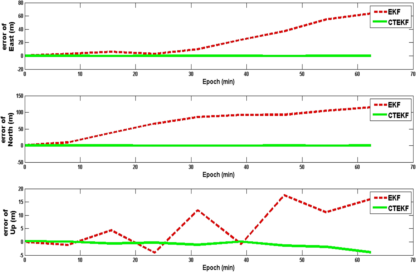
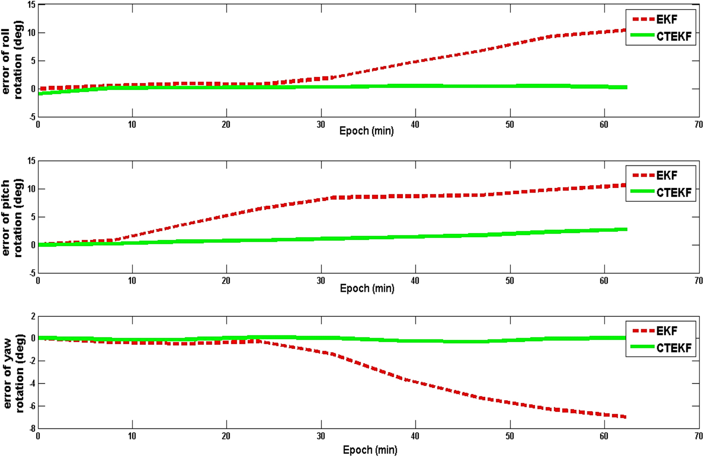
The navigation solution was improved as shown in Figures 8 and 9 and Table 3. The time series of position and attitude (rotation) prediction errors for the EKF and CTEKF algorithms are plotted in Figures 8 and 9 in which three position components East, North and Up, and three rotation components, Roll, Pitch and Yaw, are illustrated. As can be seen from the figures, the CTEKF algorithm shows approximately 5° improvement for attitude and approximately 10 metres for position on average in contrast to the EKF approach. Moreover, the proposed algorithm is convergent in contrast to the EKF algorithm. This situation is more significant in 3D attitude since the imposed constraints refer to angles.
Position prediction error time series.

Attitude (rotation) prediction error time series.

The percentage of navigational error for two filters in three directions.

5. CONCLUSIONS
In this paper, the EKF algorithm has been applied to dynamic error-in-variables models, it has been shown that adding generalised quadratic constraints improves model output. In particular, for a more appropriate modelling of an integrated direct geo-referencing problem, we found that a new algorithm named CTEKF (or its simplified version) should be used. The predicted residuals for all variables besides the variance matrix of the unknown parameters were obtained. In particular, the developed algorithm can be applied to vision-based navigation in which GNSS data may not be always available since GNSS can provide information only under ideal conditions. In other words, the system does not work very well in urban and/or canopy areas due to signal blockage and can be totally blocked if the signal is jammed. In such a case, fusing the vision and INS data by the developed CTEKF is recommended. The observation equations can be obtained from vision data while INS data provides the system equations.