1 Introduction
When an electric field is applied across a drop of fluid suspended in another fluid, a jump in electric stress is generated at the interface due to a mismatch in the electrical properties between the fluids. For perfectly conducting or perfectly dielectric drops, suspended in a perfectly dielectric fluid, the resultant electric traction solely acts normal to the interface and is balanced by capillary traction due to surface tension. The electric traction is non-uniform along the interface, and consequently, the drop becomes elongated along the direction of the applied field into a prolate shape (Zeleny Reference Zeleny1917; Wilson & Taylor Reference Wilson and Taylor1925; Macky Reference Macky1931; O’Konski & Thacher Reference O’Konski and Thacher1953; Taylor Reference Taylor1964; Saville Reference Saville1997). For such systems, there is no fluid motion at steady state, and this phenomenon is called electrohydrostatics.
The problem becomes more complicated if both the fluids are weakly conducting, or leaky dielectrics. Drops of such fluids can also deform perpendicular to the applied field into oblate shapes (Allan & Mason Reference Allan and Mason1962). This was explained by Taylor (Reference Taylor1966) in his ‘leaky dielectric model’. The conductivity of such fluids is typically less than
 $10^{-9}~\text{S}~\text{m}^{-1}$
, which is, for example, very small compared to distilled water, that has a conductivity of around
 $10^{-4}~\text{S}~\text{m}^{-1}$
. Since the conductivity is not zero, however, as is the case with perfect dielectrics, charge carriers can be transported from the bulk fluids to the interface under an electric field. The characteristic time for a charge to reach the interface is given by the charge relaxation time scale,
 $t_{e(i,o)}=\unicode[STIX]{x1D700}_{i,o}/\unicode[STIX]{x1D70E}_{i,o}$
, where
 $\unicode[STIX]{x1D700}$
is the permittivity and
 $\unicode[STIX]{x1D70E}$
is the conductivity and the subscripts ‘
 $i$
’ and ‘
 $o$
’ refer to properties of the drop and the medium, respectively. The action of the imposed field on the accumulated charge at the interface generates a component of the electric stress tangential to the interface, in addition to a normal component. This requires a tangential viscous stress to balance it, which is why a flow is generated. The flow is sustained even if the system reaches a steady state, and this phenomenon is therefore referred to as electrohydrodynamics (Taylor Reference Taylor1966; Melcher & Taylor Reference Melcher and Taylor1969; Saville Reference Saville1997). A leaky dielectric drop can deform into either a prolate or an oblate shape, depending on the properties of the drop and the medium. Taylor’s small deformation theory predicts the steady state deformation of the drop to be
 $$\begin{eqnarray}D_{T}={\displaystyle \frac{9}{16(2R+1)^{2}}}\left[{\displaystyle \frac{3R(3M+2)(1-RS)}{5(M+1)}}+R^{2}(1-2S)+1\right]Ca_{E},\end{eqnarray}$$
where
 $R=\unicode[STIX]{x1D70E}_{o}/\unicode[STIX]{x1D70E}_{i}$
is the ratio of conductivity of the medium to the drop,
 $S=\unicode[STIX]{x1D700}_{i}/\unicode[STIX]{x1D700}_{o}$
is the ratio of the permittivity of the drop to the medium and
 $M=\unicode[STIX]{x1D707}_{i}/\unicode[STIX]{x1D707}_{o}$
is the ratio of viscosity of the drop to the medium, with
 $\unicode[STIX]{x1D707}$
denoting the viscosity. Note that in his original paper, Taylor had used an inverse definition of
 $M,S$
and
 $R$
. The steady state deformation is defined as
 $D_{T}=(L-l)/(L+l)$
, where
 $L$
and
 $l$
denote the semi-axes along and perpendicular to the applied field, respectively (figure 1). The electric capillary number,
 $Ca_{E}=\unicode[STIX]{x1D700}_{o}a_{0}E_{\infty }^{2}/\unicode[STIX]{x1D6FE}$
is the ratio of electric stress (
 $\unicode[STIX]{x1D700}_{o}E_{\infty }^{2}$
) to capillary stress (
 $\unicode[STIX]{x1D6FE}/a_{0}$
), where
 $a_{0}$
is the radius of the undeformed drop and
 $\unicode[STIX]{x1D6FE}$
is the interfacial tension. The capillary number is calculated based on the medium properties. The capillary number can also be defined as the ratio of the capillary time scale,
 $t_{c,o}=\unicode[STIX]{x1D707}_{o}a_{0}/\unicode[STIX]{x1D6FE}$
, which represents the time taken by the capillary force to restore the drop to its undeformed state, to the flow time scale,
 $t_{f,o}=a_{0}/U$
, where the velocity scale is obtained by balancing shear and electric stresses, and is given by
 $U=\unicode[STIX]{x1D700}_{o}\unicode[STIX]{x1D707}_{o}E_{\infty }^{2}/a_{0}$
. Taylor’s theory is valid for small values of the capillary number,
 $Ca_{E}\ll 1$
, and predicts that the drop deforms into a spheroidal shape: prolate if
 $D_{T}>0$
, and oblate if
 $D_{T}<0$
.
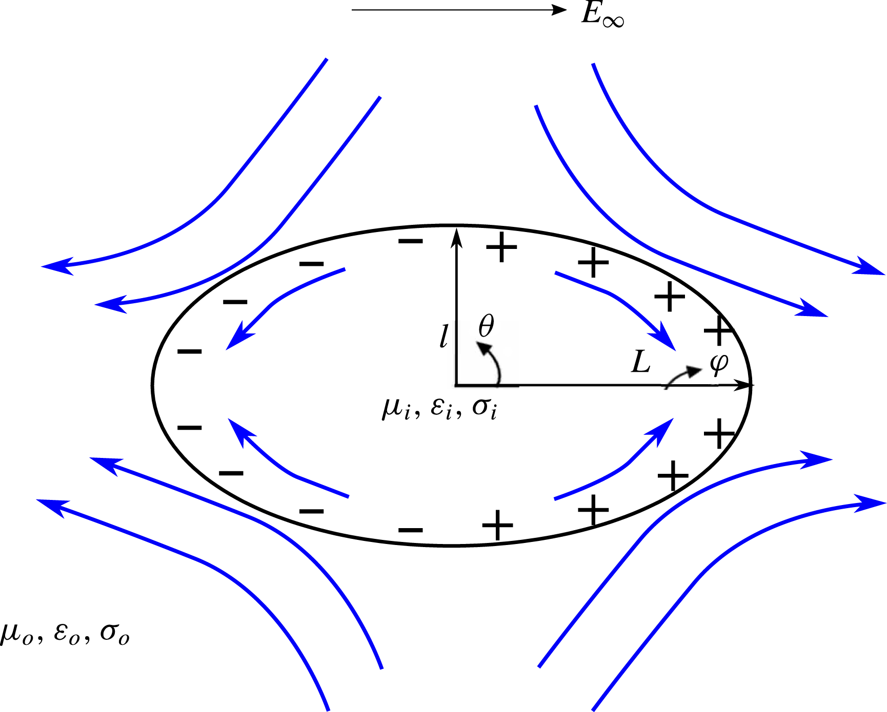
Schematic of electric field induced prolate deformation of a leaky dielectric drop. The axis of rotational symmetry,
 $\unicode[STIX]{x1D711}$
, is along the direction of the applied field. The drop of viscosity
 $\unicode[STIX]{x1D707}_{i}$
, permittivity
 $\unicode[STIX]{x1D700}_{i}$
and conductivity
 $\unicode[STIX]{x1D70E}_{i}$
is suspended in a fluid of viscosity
 $\unicode[STIX]{x1D707}_{o}$
, permittivity
 $\unicode[STIX]{x1D700}_{o}$
and conductivity
 $\unicode[STIX]{x1D70E}_{o}$
. Here, the charge relaxation time scale of the drop,
 $t_{e,i}=\unicode[STIX]{x1D700}_{i}/\unicode[STIX]{x1D70E}_{i}$
is smaller than the charge relaxation time scale of the medium,
 $t_{e,o}=\unicode[STIX]{x1D700}_{o}/\unicode[STIX]{x1D70E}_{o}$
. Consequently, the charging of the interface is controlled by the drop, and the induced flow is directed from the equator (
 $\unicode[STIX]{x1D703}=\unicode[STIX]{x03C0}/2,3\unicode[STIX]{x03C0}/2$
) to the poles (
 $\unicode[STIX]{x1D703}=0,\unicode[STIX]{x03C0}$
). The curved arrows denote the direction of fluid flow.

Taylor’s small deformation theory qualitatively explains oblate and prolate deformations based on the properties of the fluids. It predicts accurate values for the deformation at small
 $Ca_{E}$
, however a quantitative match at larger
 $Ca_{E}$
with experiments is poor, with the theory underestimating the measured deformations (Torza et al.
Reference Torza, Cox and Mason1971; Vizika & Saville Reference Vizika and Saville1992; Salipante & Vlahovska Reference Salipante and Vlahovska2010). The inclusion of higher-order terms to Taylor’s model (Ajayi Reference Ajayi1978) does not resolve this discrepancy. Droplet deformation at larger
 $Ca_{E}$
has received attention in numerical studies to determine the steady state deformation, as well as breakup of drops (Sherwood Reference Sherwood1988; Basaran et al.
Reference Basaran, Patzek, Brenner and Scriven1995; Feng & Scott Reference Feng and Scott1996; Feng Reference Feng1999; Lac & Homsy Reference Lac and Homsy2007; Collins et al.
Reference Collins, Jones, Harris and Basaran2008; Supeene et al.
Reference Supeene, Koch and Bhattacharjee2008; Collins et al.
Reference Collins, Sambath, Harris and Basaran2013; Lanauze et al.
Reference Lanauze, Walker and Khair2015; Das & Saintillan Reference Das and Saintillan2016). At larger deformations, the drop shape may substantially deviate from a spheroid (Sherwood Reference Sherwood1988; Lac & Homsy Reference Lac and Homsy2007; Lanauze et al.
Reference Lanauze, Walker and Khair2015). Sherwood (Reference Sherwood1988) was the first to computationally study the steady shapes and breakup modes of leaky dielectric prolate drops under creeping flow conditions (i.e. the flow Reynolds numbers,
 $Re_{i,o}=\unicode[STIX]{x1D70C}_{i,o}a_{0}U/\unicode[STIX]{x1D707}_{i,o}$
was assumed to be zero) using the boundary integral method. In his study, the viscosity of the drop was considered to be equal to that of the medium, and the effect of
 $R$
and
 $S$
on the final state of the drop was analysed. Sherwood identified two modes of breakup: end pinching, where a drop elongates into a cylindrical thread and develops two or more lobes which eventually detach from the thread; and breakup by pointed ends. He concluded that pointed ends are observed when the permittivity of the drop is high compared to that of the medium, and end pinching is observed when the conductivity of the drop is higher than that of the medium. Lac & Homsy (Reference Lac and Homsy2007) performed boundary integral computations to investigate the behaviour of a leaky dielectric drop in a wider parameter space, by varying
 $M,S$
and
 $R$
. Both prolate and oblate deformations were considered in their study, which identified various steady and unsteady shapes, some characterized by multiple lobes. The effect of fluid inertia was probed by Feng & Scott (Reference Feng and Scott1996), Feng (Reference Feng1999) and Nganguia et al. (Reference Nganguia, Young, Layton, Lai and Hu2016), where finite values of
 $Re_{i,o}$
were considered. These studies show that for cases with realistic values of fluid properties and applied fields, where the flow Reynolds number,
 $Re\sim O(1)$
, inertia does not play a significant role in leaky dielectric prolate drop systems.
Although the studies by Sherwood (Reference Sherwood1988) and Lac & Homsy (Reference Lac and Homsy2007) dealt with leaky dielectric drops, they neglected the effects of surface charge convection, by effectively assuming that the interface is charged instantaneously, i.e. the charge relaxation time (
 $t_{e}$
) is much smaller than the flow (
 $t_{f}$
) and capillary (
 $t_{c}$
) times. This assumption simplifies the analysis by decoupling the electrostatic and fluid flow problems; however, in experiments the value of the charge relaxation time scale can be comparable to the flow and capillary time scales (Lanauze et al.
Reference Lanauze, Walker and Khair2015). Moreover, including a non-zero
 $t_{e}$
is important to predict electrohydrodynamic tip streaming of films and drops of leaky dielectric fluids. The size of the drops that are shed as a result of tip streaming, and the charge carried by the daughter drops depend on
 $t_{e}$
(Collins et al.
Reference Collins, Jones, Harris and Basaran2008, Reference Collins, Sambath, Harris and Basaran2013). Surface charge convection is quantified by the electric Reynolds number,
 $Re_{E(i,o)}=t_{e(i,o)}/t_{f(i,o)}=\unicode[STIX]{x1D700}_{i,o}^{2}E_{\infty }^{2}/\unicode[STIX]{x1D707}_{i,o}\unicode[STIX]{x1D70E}_{i,o}$
(Melcher & Taylor Reference Melcher and Taylor1969). The experiments of Salipante & Vlahovska (Reference Salipante and Vlahovska2010) showed that charge convection affects the onset of electrorotation for oblate drops, and possibly contributes to the hysteresis observed in the transition from axisymmetric to asymmetric shapes of the drops. The computations of Lanauze et al. (Reference Lanauze, Walker and Khair2015) and Das & Saintillan (Reference Das and Saintillan2016) demonstrated that surface charge convection leads to the development of ‘charge shocks’ near the equator of oblate drops, where steep gradients develop in the surface charge density profile. The effect of surface charge convection was also incorporated in the works of Feng (Reference Feng1999), Supeene et al. (Reference Supeene, Koch and Bhattacharjee2008) and Fernandez (Reference Fernandez2013). These studies concluded that surface charge convection reduces the steady deformation of oblate drops; enhances the steady deformation of prolate drops and that accounting for surface charge convection is important to characterize the transient dynamics of the drop.
In this work, we demonstrate that surface charge convection plays a more profound role for prolate drops than just enhancing the steady state deformation, as has been previously reported (Feng Reference Feng1999; Supeene et al.
Reference Supeene, Koch and Bhattacharjee2008; Fernandez Reference Fernandez2013). Prolate drops can support flows that are directed from the equator to the poles of the drop (figure 1), as well as flows from the poles to the equator. Through boundary integral computations, we show that in the former case, surface charge convection can lead to an abrupt transition in breakup mode from end pinching to breakup by the formation of conical ends. We mainly focus on drops having the same viscosity as the medium (
 $M=1$
) and study the breakup modes of the drops as the electric Reynolds number is increased from zero to finite values. In § 2, we formulate the problem of interest, and outline the governing equations and the numerical scheme employed. In § 3 we discuss the two flow profiles that can be supported by prolate drops. In § 4, we provide the results of our work. In § 5, we discuss the experimental relevance of our computations. In § 6, we provide the conclusion of our work.
2 Problem formulation
Consider an initially uncharged weakly conducting drop of initial radius
 $a_{0}$
suspended in a weakly conducting medium (figure 1). The drop and medium have the same density and same viscosity. A uniform direct current (DC) field,
 $\boldsymbol{E}_{\boldsymbol{\infty }}$
, is applied, which induces flow in both the fluids. Prolate drops can experience flows directed either from the equator (
 $\unicode[STIX]{x1D703}=\unicode[STIX]{x03C0}/2,3\unicode[STIX]{x03C0}/2$
) to the poles (
 $\unicode[STIX]{x1D703}=0,\unicode[STIX]{x03C0}$
) of the drop, or vice versa. The direction of the fluid flow depends on the charge relaxation time scales of the drop and the medium. If
 $t_{e,i}<t_{e,o}$
, the flow is from the equator to the poles (Prolate A, or ‘
 $PR_{A}$
’ drops), and if
 $t_{e,i}>t_{e,o}$
, the flow runs from the poles to the equator (‘
 $PR_{B}$
’ drops). In this study, we will predict the drops to deform into non-spheroidal shapes, with multiple lobes. For such shapes, it is difficult to choose a semi-minor axis to quantify the deformation of the drop, per Taylor’s definition. Hence, the deformation is defined as
 $D=L/a_{0}$
, where
 $L$
denotes the half-length of the drop, and is equivalent to the semi-axis along the electric field used in Taylor’s definition. The effect of charge convection, characterized by
 $Re_{E}$
, on the breakup mode of the drop is quantified.
The electrohydrodynamic problem requires in principal the calculation of the electric field and the fluid flow inside and outside the drop, and the shape of the drop with time. We employ the boundary integral method to solve this problem. This requires the solution of the field and flow at the interface only, thereby reducing the dimensionality of the problem and hence the computational cost (Youngren & Acrivos Reference Youngren and Acrivos1975; Rallison Reference Rallison1981; Stone & Leal Reference Stone and Leal1990). Coupling between the electric field and fluid flow occurs at the interface due to the convection of charge by the electrohydrodynamic flow. This is accounted for through the interfacial charge conservation equation. We now present the governing equations. Henceforth, a superscript ‘*’ denotes a dimensional variable, and a lack of the superscript denotes a physical parameter, scale, dimensionless group or the dimensionless version of a dimensional variable.
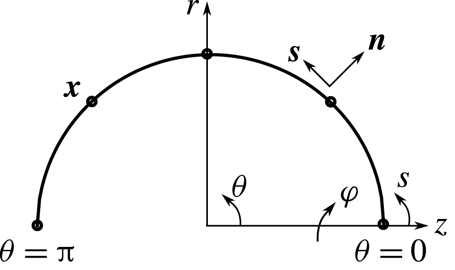
Schematic showing the discretization of the undeformed drop, the unit tangential (
 $\boldsymbol{s}$
) and normal (
 $\boldsymbol{n}$
) vectors, the continuous tangential coordinate (
 $s$
) and a fixed source point on the interface (
 $\boldsymbol{x}$
).

2.1 Electric field
The first step is to solve for the electric field and electric stress at the interface. The electric field is irrotational, and since the drop is electrically neutral, Gauss’s law for electrostatics reduces to the Laplace equation for the inner and outer electrostatic potentials, giving
 $\unicode[STIX]{x1D6FB}^{\ast 2}\unicode[STIX]{x1D719}_{i,o}^{\ast }=0$
, with the electric fields given by
 $\boldsymbol{E}_{\boldsymbol{i},\boldsymbol{o}}^{\ast }=-\unicode[STIX]{x1D735}^{\ast }\unicode[STIX]{x1D719}_{i,o}^{\ast }$
(Baygents & Saville Reference Baygents and Saville1990; Stone et al.
Reference Stone, Lister and Brenner1999; Lac & Homsy Reference Lac and Homsy2007; Lanauze et al.
Reference Lanauze, Walker and Khair2015). The electric field in the medium satisfies the condition
 $\boldsymbol{E}_{\boldsymbol{o}}^{\ast }=-\unicode[STIX]{x1D735}^{\ast }\unicode[STIX]{x1D719}_{o}^{\ast }\rightarrow \boldsymbol{E}_{\boldsymbol{\infty }}$
at large distances from the drop. In addition, the field also satisfies the interface conditions of continuity in the tangential component of the electric field, and a jump in the normal electric displacement due to the accumulation of interfacial charge (Baygents & Saville Reference Baygents and Saville1990; Lac & Homsy Reference Lac and Homsy2007; Lanauze et al.
Reference Lanauze, Walker and Khair2015), namely,
 $$\begin{eqnarray}E_{t,o}^{\ast }=E_{t,i}^{\ast },\end{eqnarray}$$
and
 $$\begin{eqnarray}\unicode[STIX]{x1D700}_{o}E_{n,o}^{\ast }-\unicode[STIX]{x1D700}_{i}E_{n,i}^{\ast }=q^{\ast },\end{eqnarray}$$
where
 $E_{t(i,o)}^{\ast }=\boldsymbol{E}_{\boldsymbol{i},\boldsymbol{o}}^{\ast }\boldsymbol{\cdot }\boldsymbol{s}$
is the tangential component of the inner and outer electric fields, respectively, and
 $\boldsymbol{s}$
is a unit tangent vector, positive in the counterclockwise direction. The normal component of the electric field is given by
 $E_{n(i,o)}^{\ast }=\boldsymbol{E}_{\boldsymbol{i},\boldsymbol{o}}^{\ast }\boldsymbol{\cdot }\boldsymbol{n}$
, where
 $\boldsymbol{n}$
is a unit normal vector, positive in the outward direction (figure 2), and
 $q^{\ast }$
is the interfacial charge density.
We first non-dimensionalize the problem. Distance is non-dimensionalized with the radius of the undeformed drop,
 $a_{0}$
. The magnitude of the applied electric field,
 $E_{\infty }$
, is used to normalize the electric fields. Surface charge density is rendered dimensionless using
 $\unicode[STIX]{x1D700}_{o}E_{\infty }$
, and time is normalized by the capillary time,
 $t_{c}=\unicode[STIX]{x1D707}_{o}a_{0}/\unicode[STIX]{x1D6FE}$
. The fluid flow is driven by the electric stress acting at the interface. Thus, the velocity scale is obtained by balancing the electrical stress with the viscous shear stress, giving
 $U=\unicode[STIX]{x1D700}_{o}E_{\infty }^{2}a_{0}/\unicode[STIX]{x1D707}_{o}$
. Using these scalings, the Laplace equation is recast into a non-dimensional integral equation (Stone et al.
Reference Stone, Lister and Brenner1999; Lac & Homsy Reference Lac and Homsy2007; Lanauze et al.
Reference Lanauze, Walker and Khair2015)
 $$\begin{eqnarray}\boldsymbol{E}_{\boldsymbol{\infty }}\boldsymbol{\cdot }\boldsymbol{n}(\boldsymbol{x})-{\displaystyle \frac{1}{4\unicode[STIX]{x03C0}}}\oint _{A}{\displaystyle \frac{\boldsymbol{r}\boldsymbol{\cdot }\boldsymbol{n}(\boldsymbol{x})}{r^{3}}}(E_{n,o}(\,\boldsymbol{y})-E_{n,i}(\,\boldsymbol{y}))\,\text{d}A(\,\boldsymbol{y})={\displaystyle \frac{1}{2}}[E_{n,o}(\boldsymbol{x})+E_{n,i}(\boldsymbol{x})],\end{eqnarray}$$
where
 $\boldsymbol{r}=\boldsymbol{y}-\boldsymbol{x}$
is the distance between an observer point
 $\boldsymbol{y}$
that can move along the interface and a fixed source point
 $\boldsymbol{x}$
on the interface. The integral is taken over the surface area
 $A$
of the drop. Equation (2.3) has two unknowns
 $E_{n,o}$
and
 $E_{n,i}$
. Using the dimensionless form of (2.2),
 $E_{n,i}=(E_{n,o}-q)/S$
, to substitute for
 $E_{n,i}$
, equation (2.3) can be written as (Lanauze et al.
Reference Lanauze, Walker and Khair2015)
 $$\begin{eqnarray}\displaystyle & & \displaystyle {\displaystyle \frac{S-1}{4\unicode[STIX]{x03C0}S}}\oint _{A}{\displaystyle \frac{\boldsymbol{r}\boldsymbol{\cdot }\boldsymbol{n}(\boldsymbol{x})}{r^{3}}}E_{n,o}(\,\boldsymbol{y})\,\text{d}A(\,\boldsymbol{y})+{\displaystyle \frac{S+1}{2S}}E_{n,o}(\boldsymbol{x})\nonumber\\ \displaystyle & & \displaystyle \quad =\boldsymbol{E}_{\boldsymbol{\infty }}\boldsymbol{\cdot }\boldsymbol{n}(\boldsymbol{x})-{\displaystyle \frac{1}{4\unicode[STIX]{x03C0}S}}\oint _{A}q(\,\boldsymbol{y})\,\text{d}A(\,\boldsymbol{y})+{\displaystyle \frac{1}{2S}}q(\boldsymbol{x}).\end{eqnarray}$$
To calculate the normal electric field, a knowledge of the surface charge density is required. The interface is initially uncharged, and hence
 $E_{n,o}$
and subsequently
 $E_{n,i}$
can be computed at
 $t=0$
.
After calculating the normal electric fields inside and outside the drop, the tangential fields are obtained by an integral transformation of the Laplace equation in terms of the electrostatic potential,
 $\unicode[STIX]{x1D719}_{o}$
(Pozrikidis Reference Pozrikidis2010; Lanauze et al.
Reference Lanauze, Walker and Khair2015),
 $$\begin{eqnarray}\unicode[STIX]{x1D719}_{o}(\boldsymbol{x})=\unicode[STIX]{x1D719}_{\infty }(\boldsymbol{x})+\oint _{A}{\displaystyle \frac{1}{4\unicode[STIX]{x03C0}r}}(E_{n,o}(\,\boldsymbol{y})-E_{n,i}(\,\boldsymbol{y}))\,\text{d}A(\,\boldsymbol{y}).\end{eqnarray}$$
The tangential field is obtained using
 $E_{t,o}=-\unicode[STIX]{x2202}\unicode[STIX]{x1D719}_{o}/\unicode[STIX]{x2202}s$
and (2.1). Here,
 $s$
is the tangential coordinate measured from
 $\unicode[STIX]{x1D703}=0$
(figure 2). From the normal and tangential components of the electric field inside and outside the drop, the jump in electric traction at the interface from inside the drop to outside is evaluated as
 $$\begin{eqnarray}[\unicode[STIX]{x1D749}_{\boldsymbol{e}}\boldsymbol{\cdot }\boldsymbol{n}]={\textstyle \frac{1}{2}}[(E_{n,o}^{2}-SE_{n,i}^{2})+(S-1)E_{t,o}^{2}]\boldsymbol{n}+E_{t,o}(E_{n,o}-SE_{n,i})\boldsymbol{t}=\unicode[STIX]{x0394}p_{E}\boldsymbol{n}+qE_{t,o}\boldsymbol{t},\end{eqnarray}$$
where
 $\unicode[STIX]{x1D749}_{\boldsymbol{e}(\boldsymbol{i},\boldsymbol{o})}=\boldsymbol{E}_{\boldsymbol{i},\boldsymbol{o}}\boldsymbol{E}_{\boldsymbol{i},\boldsymbol{o}}-E_{i,o}^{2}\boldsymbol{I}/2$
is the dimensionless form of the Maxwell stress tensor and
 $\unicode[STIX]{x1D700}_{o}E_{\infty }^{2}$
is the scale used to non-dimensionalize it. Following the notation used by Lac & Homsy (Reference Lac and Homsy2007) and Lanauze et al. (Reference Lanauze, Walker and Khair2015), the jump in normal component of the electric traction is denoted by
 $\unicode[STIX]{x0394}p_{E}$
, and is called the electric pressure, and the tangential component of the jump in electric traction, which is responsible for maintaining a flow, is
 $qE_{t,o}$
.
2.2 Fluid flow
The flow of fluid is sustained by the tangential component of the electrical stress. In this study, we assume creeping flow,
 $Re=0$
. Although in experiments
 $Re\sim O(1)$
(Lanauze et al.
Reference Lanauze, Walker and Khair2015), the computations of Feng & Scott (Reference Feng and Scott1996) and Nganguia et al. (Reference Nganguia, Young, Layton, Lai and Hu2016) show that including fluid inertia at
 $Re\sim O(1)$
makes little difference in the steady state deformations from the results obtained using
 $Re=0$
. Thus, the flow satisfies the equation of continuity, along with Stokes equations, which when cast as integral equations in a dimensionless form becomes (Pozrikidis Reference Pozrikidis1992)
 $$\begin{eqnarray}\boldsymbol{u}_{\boldsymbol{o}}(\boldsymbol{x})=-{\displaystyle \frac{1}{8\unicode[STIX]{x03C0}}}\oint _{A}\unicode[STIX]{x0394}\boldsymbol{f}(\,\boldsymbol{y})\boldsymbol{\cdot }\boldsymbol{J}(\,\boldsymbol{y},\boldsymbol{x})\,\text{d}A(\,\boldsymbol{y}),\end{eqnarray}$$
where
 $\boldsymbol{J}$
and
 $\boldsymbol{K}$
denote the free-space Green’s functions for velocity and stress, respectively, and
 $$\begin{eqnarray}\unicode[STIX]{x0394}\boldsymbol{f}={\displaystyle \frac{2\unicode[STIX]{x1D705}_{m}\boldsymbol{n}}{Ca_{E}}}-[\unicode[STIX]{x1D749}_{\boldsymbol{e}}\boldsymbol{\cdot }\boldsymbol{n}]\end{eqnarray}$$
is the jump in hydrodynamic traction at the interface, where
 $\unicode[STIX]{x1D705}_{m}$
is the mean curvature defined as (Feng Reference Feng1999)
 $$\begin{eqnarray}\unicode[STIX]{x1D705}_{m}\boldsymbol{n}={\displaystyle \frac{1}{2}}\left[{\displaystyle \frac{\text{d}\boldsymbol{s}}{\text{d}s}}+{\displaystyle \frac{\boldsymbol{n}}{r}}{\displaystyle \frac{\text{d}z}{\text{d}s}}\right],\end{eqnarray}$$
and
 $Ca_{E}=\unicode[STIX]{x1D700}_{o}E_{\infty }^{2}a_{0}/\unicode[STIX]{x1D6FE}$
is the electric capillary number based on medium properties.
2.3 Interfacial charge conservation
After obtaining the interfacial velocity, the surface charge density is updated. This is performed using the interfacial charge conservation equation (Melcher & Taylor Reference Melcher and Taylor1969; Saville Reference Saville1997), which reads in dimensionless form,
 $$\begin{eqnarray}Sa{\displaystyle \frac{\unicode[STIX]{x2202}q}{\unicode[STIX]{x2202}t}}+Re_{E}\unicode[STIX]{x1D735}_{\boldsymbol{s}}\boldsymbol{\cdot }(\boldsymbol{u}_{\boldsymbol{o}}q)={\displaystyle \frac{E_{n,i}}{R}}-E_{n,o},\end{eqnarray}$$
where
 $Re_{E}=\unicode[STIX]{x1D700}_{o}^{2}E_{\infty }^{2}/\unicode[STIX]{x1D707}_{o}\unicode[STIX]{x1D70E}_{o}$
is the electric Reynolds number based on medium properties and
 $Sa=Re_{E}/Ca_{E}$
is the Saville number, which is the ratio of the charge relaxation time scale to the capillary time scale. The first term on the left-hand side of (2.10) represents the transient charging of the interface, i.e. the charge relaxation. The second term accounts for surface charge convection, and changes in the surface charge density due to dilation of the interface. This term couples the electric field and fluid flow equations due to the presence of
 $\boldsymbol{u}_{o}$
. The terms on the right-hand side account for the Ohmic conduction of charges from the bulk to the interface and vice versa. Finally, the interface is updated using the dimensionless kinematic condition
 $$\begin{eqnarray}{\displaystyle \frac{\text{d}\boldsymbol{x}}{\text{d}t}}=Ca_{E}(\boldsymbol{u}_{\boldsymbol{o}}\boldsymbol{\cdot }\boldsymbol{n})\boldsymbol{n}.\end{eqnarray}$$
2.4 Numerical scheme
Equations (2.4), (2.5) are (2.7) are solved sequentially via the boundary element method. The details of the numerical method have been provided in an earlier publication from our group (Lanauze et al.
Reference Lanauze, Walker and Khair2015), and will therefore only be briefly discussed here. The field and flow are assumed to be axisymmetric, allowing an analytical integration over the azimuth, which reduces the surface integrals to line integrals over the contour of the drop. The top half of the drop is partitioned into
 $N$
elements. This creates
 $N+1$
nodes, which are called source points, and whose coordinates are denoted by
 $\boldsymbol{x}$
. All functions are interpolated as cubic splines with respect to
 $s$
. The integral over the entire contour is replaced by a sum of integrals over each element. Singular terms in the integrands are subtracted out, and then added back, following standard regularization techniques (Pozrikidis Reference Pozrikidis2010). Gauss–Legendre quadrature is used to evaluate the integrals and the points at which the integrand is evaluated are termed observer points, their coordinates being denoted by
 $\boldsymbol{y}$
. After evaluating the field and flow equations, the surface charge density (2.10) and the shape of the interface (2.11) is updated using the second-order Runge–Kutta method, and the deformation of the drop at every time instant is calculated. The time step is chosen such that the volumetric flow rate across the interface, which should be identically zero to conserve mass, is at most
 $O(10^{-6})$
for the initial 20 iterations. This ensures that the computations remain stable for the selected time step, and any instability occurs due to the breakup of the drop. If the volumetric flow rate across the interface remains
 $O(10^{-6})$
or less, while the maximum value of the radial velocity keeps on decreasing and reaches
 $O(10^{-4})$
or less, we conclude that the drop has attained a steady shape. If the volumetric flow rate slowly starts to increase, along with an increase in the maximum value of the radial velocity, we conclude that the drop shape is unsteady, and it will eventually breakup. The boundary integral method cannot track the interface after the drop breaks, and in this case, the results are reported at a time instant very close to breakup, where the ratio of volumetric flow rate across the interface to the initial volumetric flow rate is
 $O(10^{2})$
. For all our computations, the top half of the drop was divided into 150 elements, and the time step size was taken to be 0.05. These values were chosen after performing a convergence analysis, the results of which are given in the Appendix.
3 Flow in prolate drops
At
 $Ca_{E}\ll 1$
, and neglecting surface charge convection,
 $Re_{E}=0$
, the electrohydrodynamic problem has been solved analytically for DC electric fields (Taylor Reference Taylor1966). Depending on the ratios
 $M,S$
and
 $R$
, the drop can deform into prolate or oblate shapes, or even remain spherical. Oblate drops only support flows directed from the poles to the equator, whereas depending on the ratios, prolate drops can support flows directed from the equator to the poles (
 $PR_{A}$
drops), as well as flows directed from the poles to the equator (
 $PR_{B}$
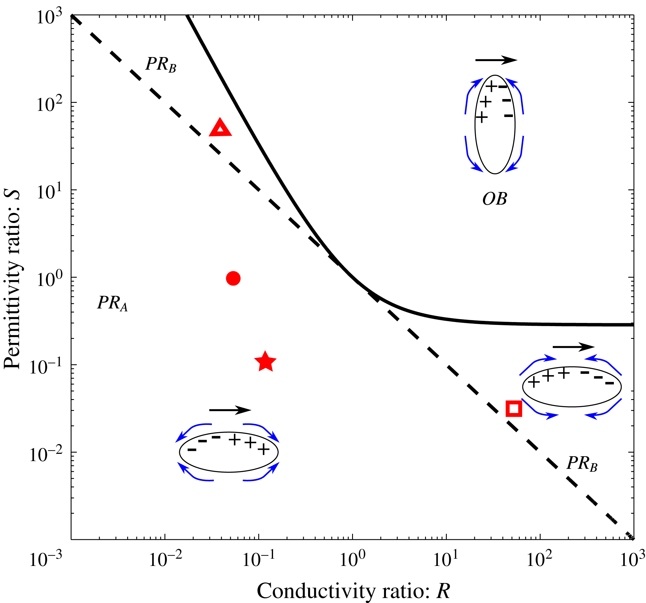
drops). Figure 3 depicts various behaviours of the drop in the (
 $R-S$
) space when
 $M=1$
. This figure has been previously shown by Torza et al. (Reference Torza, Cox and Mason1971), Baygents et al. (Reference Baygents, Rivette and Stone1998) and Lac & Homsy (Reference Lac and Homsy2007); it is reproduced here to provide a context for our nonlinear computations.
(
 $R-S$
) parameter space diagram for
 $M=1$
. The solid line distinguishes regions showing prolate deformation from regions showing oblate deformation. Points along the solid line remain spherical under an applied electric field (at small
 $Ca_{E}$
). The dotted line separates drops showing prolate A (
 $PR_{A}$
) behaviour from drops showing prolate B (
 $PR_{B}$
) behaviour. The four symbols on the diagram represent the four systems considered in this study. The curved arrows around the drops show the direction of the induced flow in each of these regions. The electric field is applied from left to right and is shown by straight arrows above the drops.

When the charge relaxation time scale of the drop is smaller than that of the medium (
 $RS<1$
), the charging of the interface is controlled by the drop. The interface gets charged in a fashion depicted by the
 $PR_{A}$
region of figure 3. This results in an electric stress, whose tangential component acts from the equator to the poles, giving rise to fluid flow in that direction. Regardless of the value of
 $M$
, prolate A behaviour occurs when
 $RS<1$
, in the region below the dashed line. The locus of the solid line is (Torza et al.
Reference Torza, Cox and Mason1971)
 $$\begin{eqnarray}RS=1+{\displaystyle \frac{5(1+M)}{16+19M}}{\displaystyle \frac{(R-1)^{2}}{R}},\end{eqnarray}$$
and along this line the drop remains spherical. This line also demarcates regions of oblate deformation from regions of prolate deformation. In the region between the solid line and the dashed line, i.e. where
 $$\begin{eqnarray}1<RS<1+{\displaystyle \frac{5(1+M)}{16+19M}}{\displaystyle \frac{(R-1)^{2}}{R}},\end{eqnarray}$$
the drop deforms into prolate shapes, but the flow is directed from the poles to the equator. In this region
 $RS>1$
, and the charging of the interface is controlled by the medium. The interface charge distribution now gives rise to an electrical stress whose tangential component is directed from the poles to the equator, thus resulting in a similar flow direction. These are the results of small deformation theory, and give a first-order estimate of the induced flow direction. The flow profile is expected to deviate when deformations are substantial and drop shapes become non-spheroidal. However, understanding the flow direction at small
 $Ca_{E}$
is important to draw conclusions on the mode of breakup of prolate drops at larger
 $Ca_{E}$
.
4 Results
The effect of surface charge convection on prolate A and prolate B drops is studied. We are interested in understanding how charge convection affects the breakup modes of these drops. The response of the drop depends on the ratios of viscosity, permittivity and conductivity, i.e.
 $M,S$
and
 $R$
; hence the computational parameter space is large. For the most part of this study, we assume
 $M=1$
, and choose different combinations of
 $S$
and
 $R$
, so as to cover different regions of the
 $R-S$
parameter space. Here, we present results on two prolate A drops, and two prolate B drops; the
 $R$
and
 $S$
values for these drops are shown in figure 3. Later, we provide a short discussion for cases where
 $M\neq 1$
.
4.1 Prolate A drops
The validity of our computational method with and without surface charge convection was established in a previous publication from our group (Lanauze et al.
Reference Lanauze, Walker and Khair2015) by comparing the results of a system with
 $(M,S,R)=(1,0.5,100)$
to the results of Feng (Reference Feng1999). Here, we first choose a system with
 $(M,S,R)=(1,1,0.05)$
, which corresponds to the filled circle symbol in figure 3, and was studied by Sherwood (Reference Sherwood1988) for the case
 $Re_{E}=0$
. This system deforms into a prolate shape and undergoes breakup at
 $Ca_{E}=0.28$
for
 $Re_{E}=0$
. Computations were performed at this value of
 $Ca_{E}$
, with
 $Re_{E}$
increasing from zero to finite values. The results are shown in figure 4.
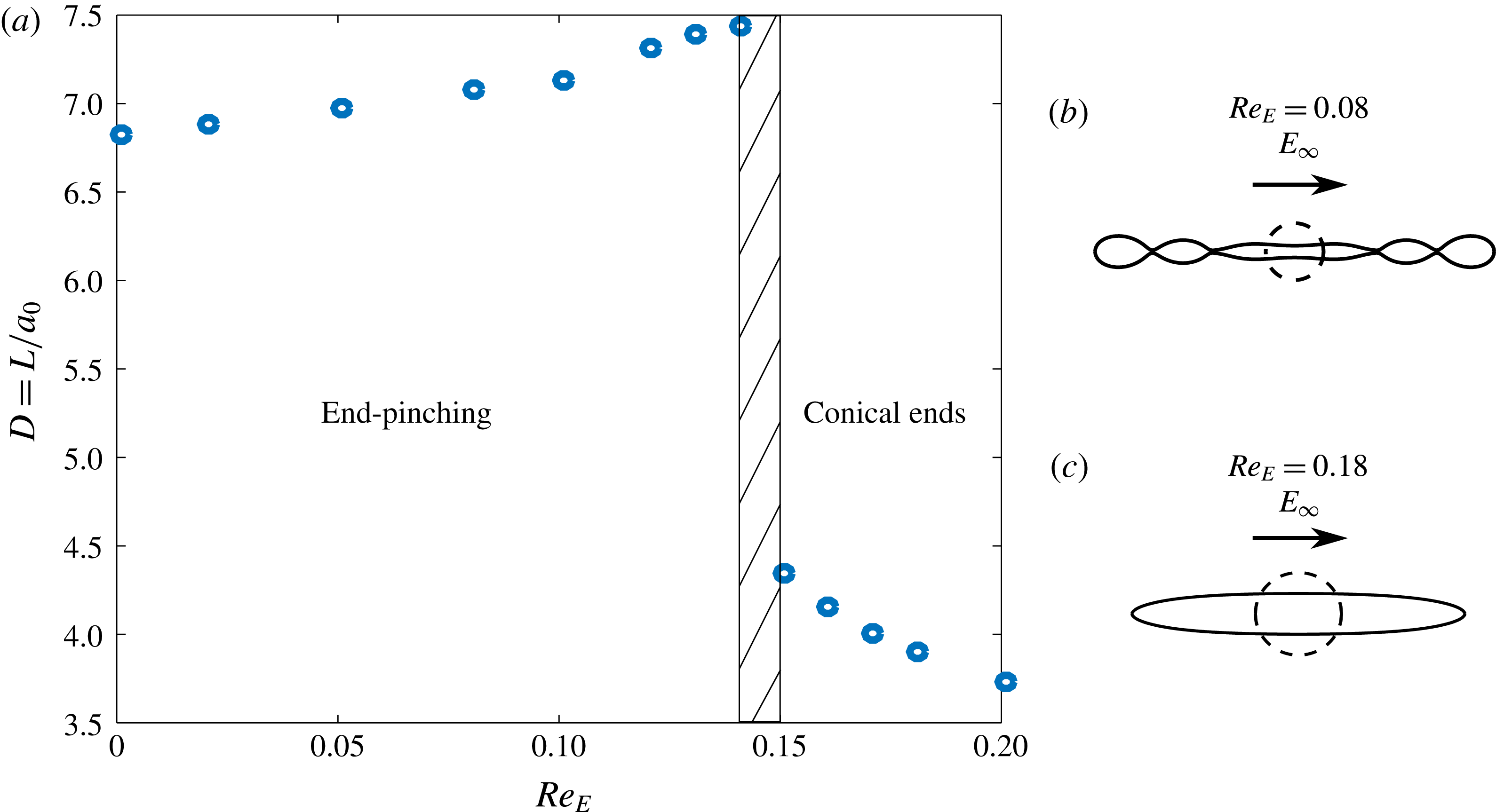
(a) Deformation,
 $D=L/a_{0}$
versus electric Reynolds number,
 $Re_{E}$
at
 $Ca_{E}=0.28$
and
 $(M,S,R)=(1,1,0.05)$
, showing the effect of surface charge convection on the breakup mode of a prolate A drop. The breakup mode changes from end pinching to breakup by conical end formation over a narrow range of
 $Re_{E}$
, as shown by the dashed region. The panel (b,c) shows the shape of the drop just before breakup at (b)
 $Re_{E}=0.08$
; and (c) at
 $Re_{E}=0.18$
, with the dotted circle representing the shape of the undeformed drop. The black arrow above the drops shows the direction of the applied electric field.

At
 $Re_{E}=0$
, the drop initially stretches into a long cylinder. After some time, bulbs form at the two ends, being connected by a thin thread of the fluid. As time progresses, the connecting thread of fluid develops more bulbs, and forms a multi-lobed structure. Eventually, the bulbs pinch off from the thread. This mechanism of breakup is called end pinching. The shape of the drop before breakup (figure 4
b) is similar to the result of Sherwood (Reference Sherwood1988) (figure 8 of that paper). As
 $Re_{E}$
is increased from zero, the mode of breakup remains the same, and the drop elongates slightly more before finally breaking. This trend continues until
 $Re_{E}=0.14$
. At
 $Re_{E}=0.15$
, the mode of breakup changes dramatically: the ends form conical tips, instead of bulbous ends. Increasing
 $Re_{E}$
further does not change the mode of breakup, but the final deformation before breakup decreases. The only parameter that was changed in the computations was the electric Reynolds number, which quantifies the strength of charge convection. Thus, surface charge convection changes the breakup mode of this drop from end pinching to the formation of conical ends at an
 $Re_{E}$
between 0.14 and 0.15 and
 $Ca_{E}=0.28$
.
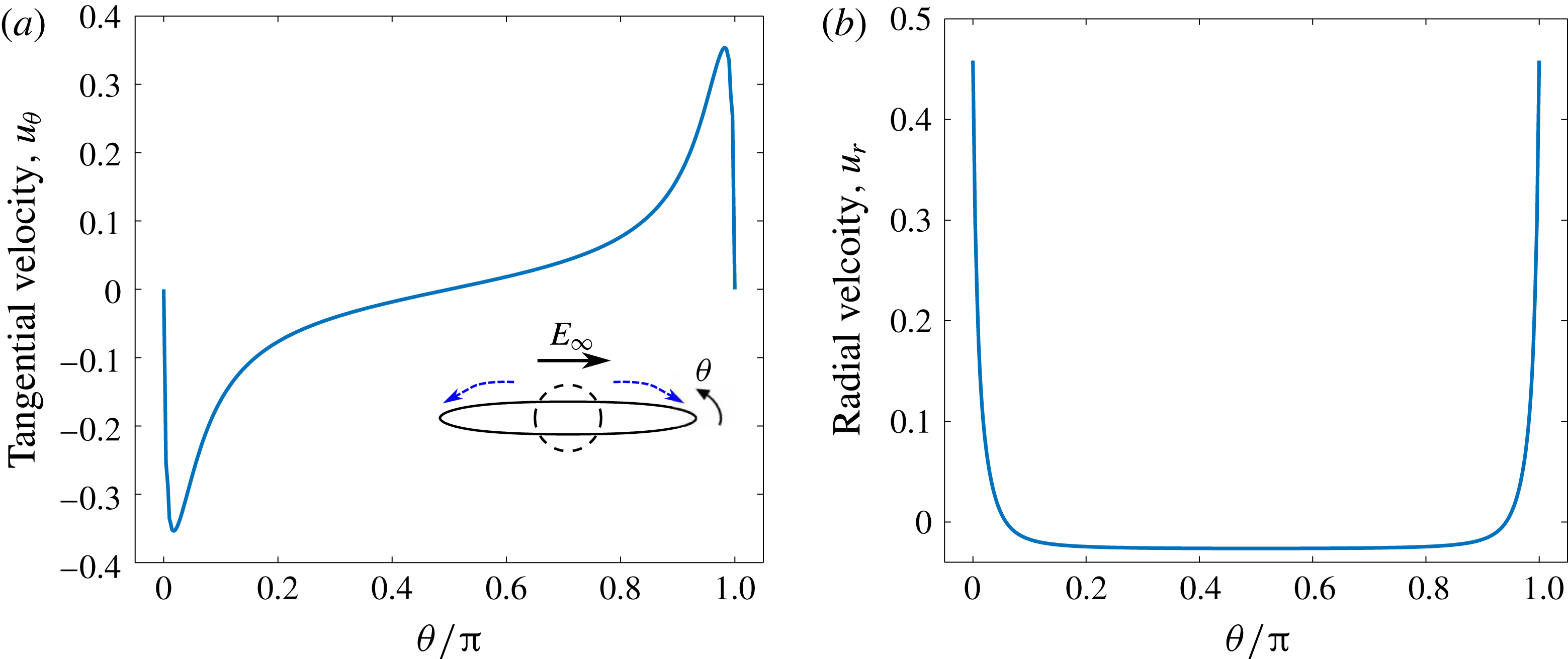
Interfacial velocity profile for a prolate A drop
 $(M,S,R=1,1,0.05)$
just before breakup. Here,
 $Ca_{E}=0.28$
and
 $Re_{E}=0.18$
. The drop breaks by the formation of pointed ends. (a) Dimensionless tangential velocity profile. The inset shows the drop shape before breakup, the dashed circle is the shape of the undeformed drop, and the dotted arrows above the drop show the direction of flow. (b) Dimensionless radial velocity profile.

To understand why a transition in breakup mode takes place, consider the jump in the electrical stress at the poles (
 $\unicode[STIX]{x1D703}=0,\unicode[STIX]{x03C0}$
) of the drop. Here, the tangential component of the electric field vanishes, and thus there is no jump in the tangential electric stress (2.6). Substituting the condition for the discontinuity in normal electric field at the interface, the electric pressure at the poles is given by
 $$\begin{eqnarray}[\unicode[STIX]{x1D749}_{\boldsymbol{e}}\boldsymbol{\cdot }\boldsymbol{n}]=\unicode[STIX]{x0394}p_{E}={\displaystyle \frac{q}{2}}(q+2SE_{n,i}),\end{eqnarray}$$
and it varies with the square of the surface charge density,
 $q$
. The electric pressure drives the drop to breakup, while the capillary stress tends to restore its spherical shape. For the system being studied, the tangential velocity profile (figure 5
a) suggests that the flow occurs from the equator to the poles of the drop, and the radial velocity profile (figure 5
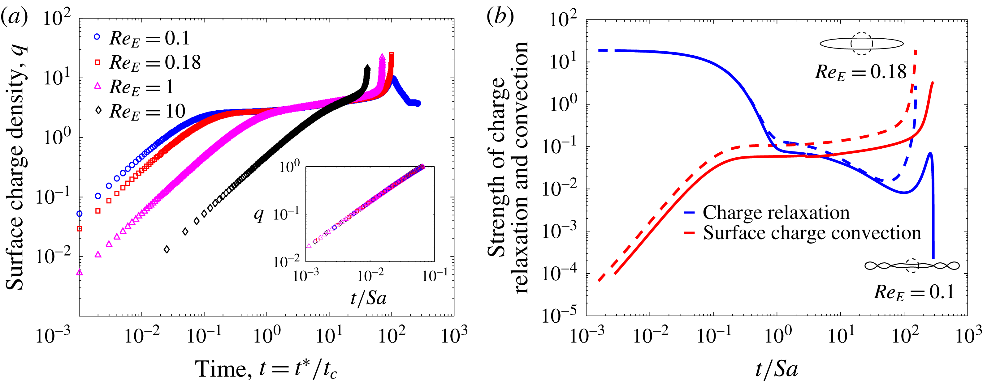
b) shows that the normal component of the velocity is very small at all points on the interface, except at the poles, where it rises sharply to values almost two orders of magnitude higher than at other points on the interface. Thus, the formation of pointed tips is accompanied by flow towards the tips of the drop. We hypothesize that the transition in the breakup mode is caused by the accumulation of surface charge at the poles due to increased charge convection by the electrohydrodynamic flow at higher
 $Re_{E}$
. The evolution of the surface charge density for a drop breaking via end pinching (
 $Re_{E}=0.1$
), and via the formation of conical ends (
 $Re_{E}=0.18,1$
and
 $10$
) is shown in figure 6(a). When the field is turned on, the interface starts acquiring charge. Initially, the surface charge density evolves in a similar fashion for all the cases. At this early stage of charging, the drop behaves as a perfect dielectric (Lanauze et al.
Reference Lanauze, Walker and Khair2013, Reference Lanauze, Walker and Khair2015), because it takes a finite amount of time for the charges to reach the interface. The strength of the fluid flow during this stage is low, and hence the surface charge convection is negligible. Figure 6(b) shows how the strength of the charge relaxation and surface charge convection (the two terms in the left-hand side of (2.10)) evolves with time. It follows that at early times, the strength of charge relaxation is at least three orders of magnitude higher than the strength of surface charge convection. During this time, charge relaxation is balanced by the discontinuity in the normal component of the electric field, and the surface charge density scales as
 $q\sim (t/Sa)[1/R-1]$
. The inset in figure 6(a) shows the early time charging at the poles for different electric Reynolds numbers. All the curves collapse when the dimensionless time is scaled by
 $Sa$
. This initial period lasts till
 $t/Sa\approx 0.1$
. After this, surface charge convection can no longer be neglected, and the early time scaling for the surface charge density no longer holds. The effect of charge convection is stronger for systems with a larger
 $Re_{E}$
(figure 6
b). Thus, drops with different values of the electric Reynolds number get charged differently after the initial period, and the distribution of surface charge density is affected by the strength of surface charge convection.
(a) Evolution of surface charge density and (b) strength of charge relaxation and surface charge convection at the poles (
 $\unicode[STIX]{x1D703}=0$
). For (b), the solid curve represents a drop breaking via end pinching (
 $Re_{E}=0.1$
) and the dashed curve represents a drop breaking via the formation of conical ends (
 $Re_{E}=0.18$
).

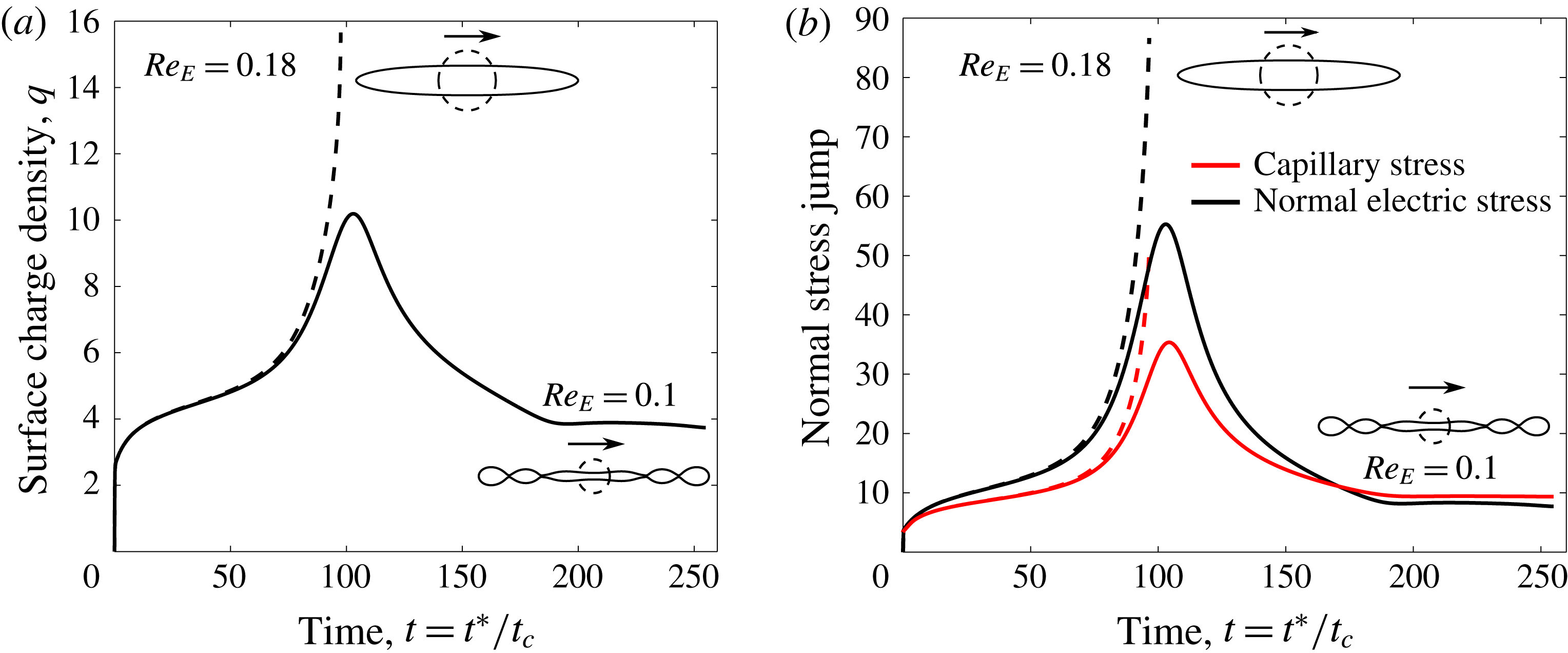
(a) Evolution of surface charge density and (b) jump in the normal component of the electric and capillary stress at the pole (
 $\unicode[STIX]{x1D703}=0$
). The solid curve represents a drop breaking via end pinching (
 $Re_{E}=0.1$
), and the dashed curve represents a drop breaking via the formation of conical ends (
 $Re_{E}=0.18$
).

Figure 7 shows the evolution of surface charge density, and the jump in the normal electric and capillary stress at the poles of the drop, for the two modes of breakup (end pinching for
 $Re_{E}=0.1$
and conical ends formation for
 $Re_{E}=0.18$
). As time progresses, the surface charge density at the poles increases for both the cases. After surface charge convection becomes comparable to the other terms in (2.10), the charge carriers are convected more strongly to the poles for the system with a larger electric Reynolds number (
 $Re_{E}=0.18$
). This system shows a monotonic increase in the surface charge density at the poles, and correspondingly, the electric pressure (figure 7
b). To balance the electric pressure, the capillary stress also increases monotonically, and as a result, the curvature at the pole increases. Eventually the electric pressure dominates and the drop breaks via the formation of pointed ends. In contrast, for
 $Re_{E}=0.1$
, the surface charge density shows a maxima, implying that the charge carriers are convected back from the poles to points elsewhere on the interface. This suggests that there is a flow reversal occurring after a particular time. The ends of the drop develop bulbs sometime after this maxima occurs. The jump in the electric stress reaches a maximum value, after which it decreases, allowing the capillary stress to dominate at the poles. Here, the drop breaks at points on the interface where the charge carriers accumulate. Therefore, the breakup mode depends on whether the electric pressure or the capillary stress dominates at the poles.
The formation of conical tips and the evolution of the surface charge density and electric pressure at the tips resemble the onset of a conic cusping singularity, which has been observed for conducting and dielectric, inviscid fluids (Zubarev Reference Zubarev2001, Reference Zubarev2002); liquid metallic films in vacuum (Suvorov & Litvinov Reference Suvorov and Litvinov2000); films of perfectly conducting fluids in an insulating gas (Collins et al.
Reference Collins, Jones, Harris and Basaran2008); and perfectly dielectric drops in oils (Pillai et al.
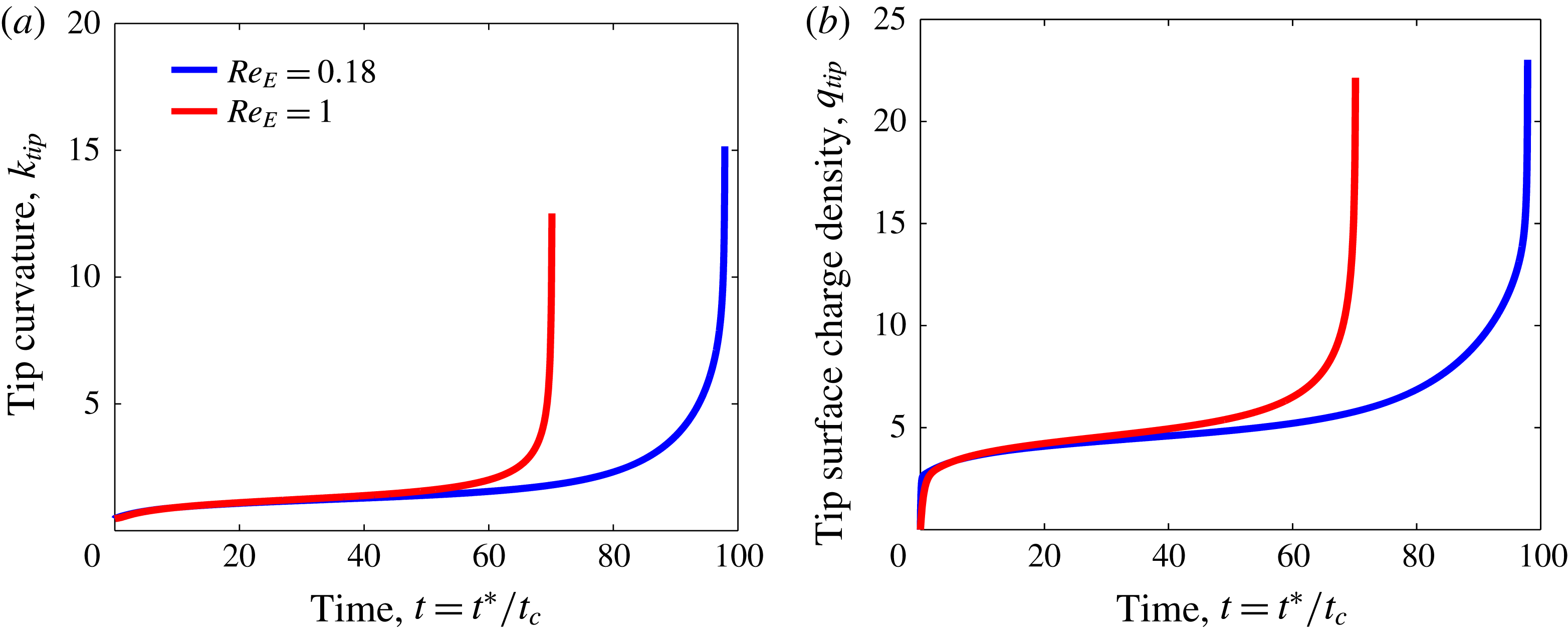
Reference Pillai, Berry, Harvie and Davidson2016), under a uniform electric field. The characteristic feature of a conic cusping singularity is that the temporal evolution of physical quantities, like the surface charge density, fluid velocity, normal electric field and the curvature at the tips exhibit a runaway behaviour. These parameters tend to become infinitely large in a finite time. Figure 8 shows the evolution of the curvature and the surface charge density at the tips for
 $Re_{E}=\{0.18,1\}$
. Both these quantities show a relatively slow growth until the onset of cusps, when they approach infinitely large values over a relatively short span of time. Further, for systems showing a conic cusping singularity, the magnitude of the electric pressure at the tips becomes much larger than the capillary force, as is exhibited in figure 7. Although the computations of Sherwood (Reference Sherwood1988) and Lac & Homsy (Reference Lac and Homsy2007) predict leaky dielectric drops to break via the formation pointed tips, an analysis of the evolution of physical parameters and the curvature at the tip was not performed. Hence, it is unclear if the conical ends observed in their studies is conic cusping. Since the flow in the drops is directed from the equator to the poles, Sherwood (Reference Sherwood1988) used the term ‘tip streaming’ to describe the breakup by pointed ends. However, tip streaming necessitates the transition of cones to fine jets, followed by the disintegration of the jet into drops of size orders of magnitude smaller than the parent drop (Basaran et al.
Reference Basaran, Patzek, Brenner and Scriven1995; Collins et al.
Reference Collins, Jones, Harris and Basaran2008, Reference Collins, Sambath, Harris and Basaran2013; Pillai et al.
Reference Pillai, Berry, Harvie and Davidson2015), and this transition has not observed in the studies of Sherwood (Reference Sherwood1988) and Lac & Homsy (Reference Lac and Homsy2007). Figures 7 and 8 indicate that the system studied here undergoes a conic cusping singularity above a critical
 $Re_{E}$
.
Evolution of the (a) curvature and (b) surface charge density at the tips of drops showing conical ends. Here,
 $(M,S,R)=(1,1,0.05)$
and
 $Ca_{E}=0.28$
.

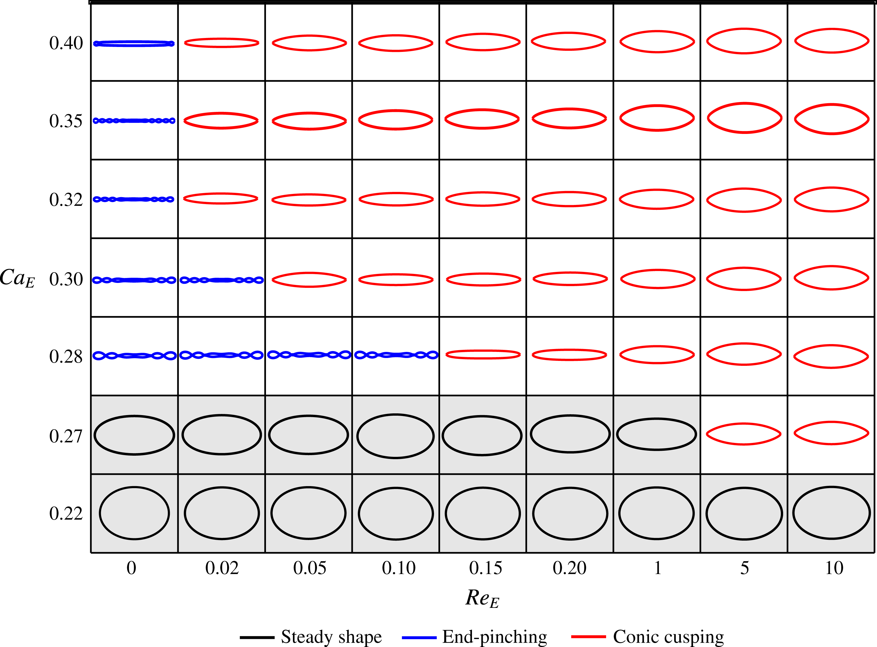
In figure 9, we present the results for the final drop state across the
 $Ca_{E}-Re_{E}$
parameter space, again for
 $(M,S,R)=(1,1,0.05)$
. From the expressions of
 $Re_{E}$
and
 $Ca_{E}$
, the magnitude of the applied electric field and the initial size of the drop are the two parameters that can be tuned to perform this parameter sweep experimentally. We find that as
 $Ca_{E}$
is increased, the value of
 $Re_{E}$
at which the transition in breakup mode occurs reduces. Drops breaking via end pinching form a higher number of lobes before breaking as
 $Ca_{E}$
increases beyond the critical capillary number. For this system, breakup via end pinching occurs over a small region in the
 $Ca_{E}-Re_{E}$
space; thus, the drop predominantly breaks via the formation of conical ends.
Final state of the drop in the
 $Ca_{E}-Re_{E}$
space for
 $(M,S,R)=(1,1,0.05)$
. Three states are identified in this diagram: steady prolate shapes, breakup by end pinching and conic cusping. The shapes have been normalized by the half-length of the drop at steady state or just before breakup. Thus, drops that deform more appear thinner in this diagram. Drops attaining steady states, or breaking via end pinching deform more as
 $Re_{E}$
,
 $Ca_{E}$
or both increase. For drops exhibiting conic cusping, the deformation just before breakup decreases as
 $Re_{E}$
,
 $Ca_{E}$
or both increase.

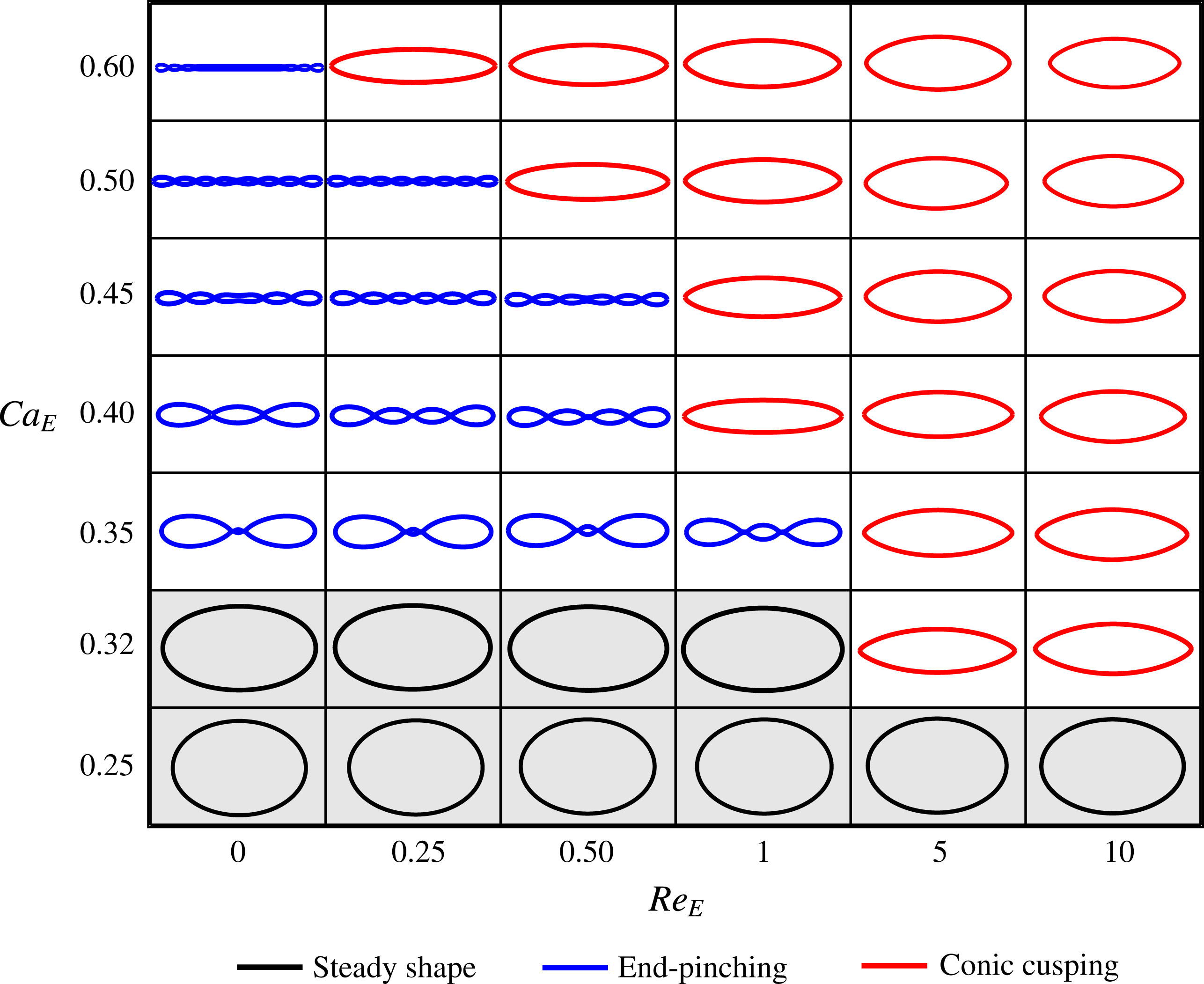
Next, we study another prolate A system with
 $(M,S,R)=(1,0.1,0.1)$
, which corresponds to the filled star symbol in figure 3, and was first examined by Lac & Homsy (Reference Lac and Homsy2007) for
 $Re_{E}=0$
only. We again start with
 $Re_{E}=0$
and probe the effect of increasing the electric Reynolds number. The results are shown in figure 10. The computations of Lac & Homsy (Reference Lac and Homsy2007) predict a critical capillary number of 0.342 for this system at
 $Re_{E}=0$
. We find that the drop breaks into two daughter drops at a critical capillary number of
 $Ca_{E}=0.35$
at
 $Re_{E}=0$
. The breakup mode observed by our computations is same as the one observed by Lac & Homsy (Reference Lac and Homsy2007) (figure 5 of their paper). Further increasing the capillary number does not alter the breakup mode, but the number of lobes before breakup increases. This is due to the fact that the destabilizing force is larger at higher capillary numbers. Thus, the drop can get elongated to a larger extent, and be more prone to capillary instability. Similar to the system depicted in figure 9, this system has a transition in breakup mode from end pinching to conic cusping beyond a certain
 $Re_{E}$
; and shows breakup via end pinching over a larger region in the
 $Ca_{E}-Re_{E}$
parameter space as compared to the system depicted in figure 9. Surface charge convection also reduces the critical capillary number for breakup; the drop exhibits conic cusping at
 $Ca_{E}=0.32$
when
 $Re_{E}=5$
, which is lower than the critical capillary number,
 $Ca_{E}=0.35$
, predicted at
 $Re_{E}=0$
.
 $Ca_{E}-Re_{E}$
parameter space plot for
 $(M,S,R=1,0.1,0.1)$
. Three states are identified in this diagram: steady prolate shapes, breakup by end pinching and conic cusping. Refer to figure 9 for details of the drop shape illustration.

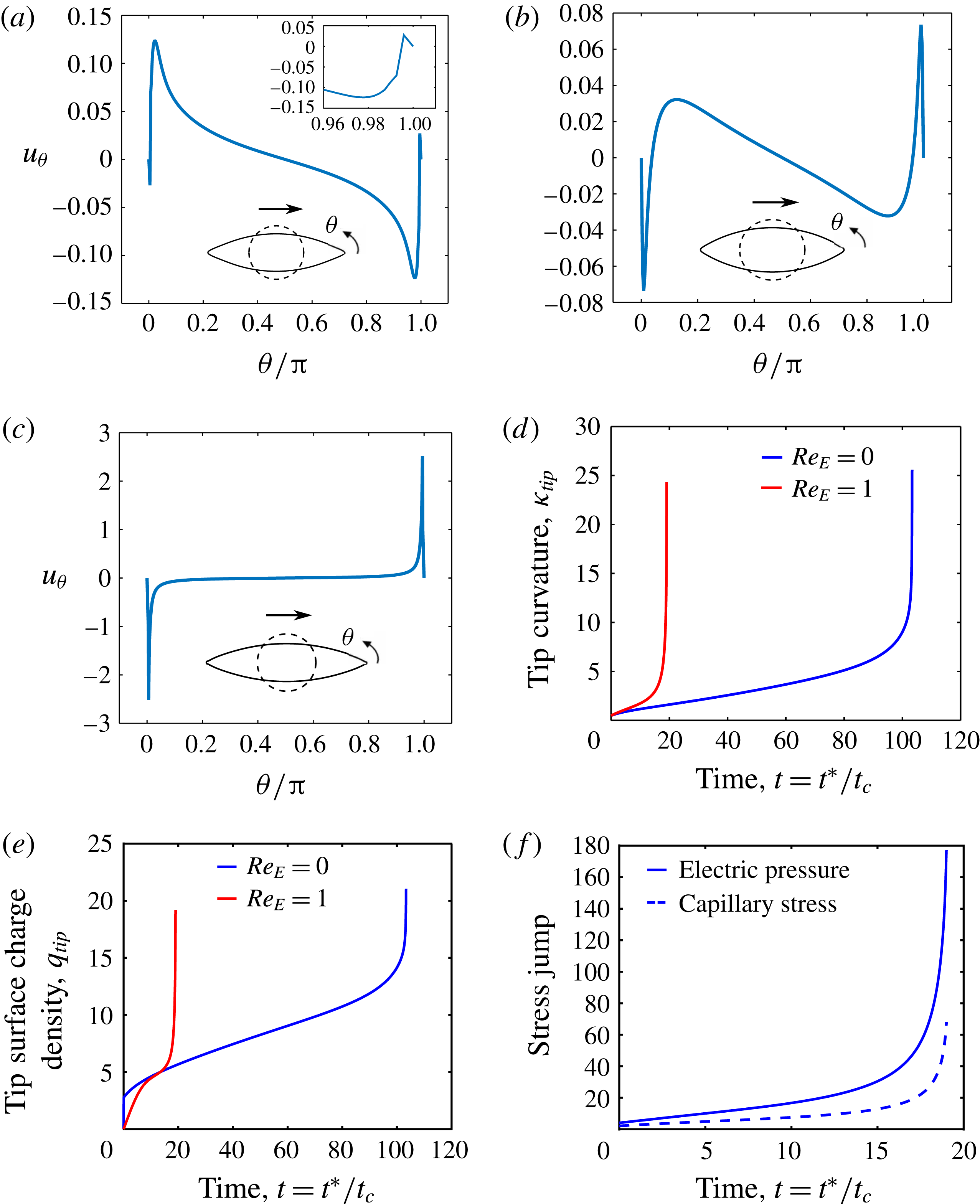
Dimensionless interfacial velocity for a prolate B system
 $(M,S,R=1,50,0.04)$
just before breakup at
 $Ca_{E}=0.46$
for (a)
 $Re_{E}=0$
, (b)
 $Re_{E}=1$
and (c)
 $Re_{E}=3$
. Evolution of (d) the curvature and (e) surface charge density at the tip of the drop at
 $Re_{E}=\{0,1\}$
. (f) Evolution of the electric pressure and the jump in capillary stress at the tips for
 $Re_{E}=1$
. The insets in the velocity profiles show the shapes of the drop just before breakup, with the dashed circles representing the shape of the undeformed drop.

In summary, for
 $PR_{A}$
drops, our computations suggest that surface charge convection abruptly changes the breakup mode from end pinching to conic cusping, and also reduces the critical capillary number for breakup. This is a consequence of the transport of charges along the interface, which in these systems, takes place from the equator to the poles. Additionally, for both systems, increasing
 $Re_{E}$
reduces the time at which breakup occurs.
4.2 Prolate B drops
We now consider prolate B drops, where small deformation theory predicts the flow to be directed from the poles to the equator. The value of our calculations here is twofold. First, we demonstrate that surface charge convection has a minor effect on the deformation of prolate B drops, as compared to prolate A drops. This highlights the important point that surface charge convection does not always lead to a significant change in drop deformation. Second, our computed steady deformations for prolate B drops are shown to compare favourably against predictions from slender-body theories (Stone et al.
Reference Stone, Lister and Brenner1999; Yariv & Rhodes Reference Yariv and Rhodes2013), which helps to assess the accuracy of the latter. Prolate B drops can be studied in experiments by choosing a pair of fluids that have a large contrast in the dielectric constant and conductivity. For example, a drop of squalane doped with polyisobutylene succinimide surfactant (OLOA 11000) in a polystyrene (PS) solution, dissolved in dimethylformamide (DMF) should show a prolate B response when subjected to an electric field. A squalane drop doped with 30 pph OLOA is characterized by
 $\unicode[STIX]{x1D707}_{i}=0.03$
Pa s,
 $\unicode[STIX]{x1D700}_{i}\sim 2$
,
 $\unicode[STIX]{x1D70E}_{i}=2.2\times 10^{-10}~\text{S}~\text{m}^{-1}$
(Lanauze Reference Lanauze2016), and for a 15 wt.% PS solution in DMF,
 $\unicode[STIX]{x1D707}_{o}=0.035$
Pa s,
 $\unicode[STIX]{x1D700}_{o}=30.2$
,
 $\unicode[STIX]{x1D70E}_{o}=7.6\times 10^{-9}~\text{S}~\text{m}^{-1}$
(Ha & Yang Reference Ha and Yang1995); yielding
 $M=0.86$
,
 $S=0.07$
and
 $R=35$
.
We first study a system with
 $(M,S,R)=(1,50,0.04)$
, which corresponds to the triangle symbol in figure 3, and was examined by Lac & Homsy (Reference Lac and Homsy2007) (figure 16 of that paper). They found the system to become unstable at a capillary number of 0.47 when
 $Re_{E}=0$
, and the drop developed pointed ends before breaking. Since the flow is from the poles to the equator, Lac & Homsy (Reference Lac and Homsy2007) did not categorize this mode of breakup as tip streaming. We find this system to become unstable at
 $Ca_{E}=0.46$
when
 $Re_{E}=0$
, and the poles develop pointed ends. The tangential velocity profile shows the appearance of stagnation points very close to the poles just before breakup (figure 11
a inset). The interfacial flow is directed from the stagnation points to the equator, as well as to the poles. Thus, charges are convected to the poles of the drop. When surface charge convection is accounted for, at non-zero
 $Re_{E}$
, the breakup mode does not change. Pointed ends are formed, there are stagnation points very close to the poles, and the flow profile suggests surface charge convection to the poles. The evolution of the curvature, surface charge density and stress jumps at the tips suggest the onset of conic cusping both at
 $Re_{E}=0$
, and at finite values of
 $Re_{E}$
(figure 11
d–f). The critical capillary number for breakup reduces, and the stagnation points move farther away from the poles as
 $Re_{E}$
increases. Similar to
 $PR_{A}$
drops, the time at which the drops undergo breakup decreases as
 $Re_{E}$
increases. At the highest values of
 $Re_{E}$
, the flow occurs from the equator to the poles, similar to that for prolate A drops (figure 11
c). A large value of
 $Re_{E}$
implies that the charge relaxation time scale is large compared to the flow time scale. The flow sets up much faster than charges arrive at the interface. The drop behaves as a perfect dielectric at initial times (Lanauze et al.
Reference Lanauze, Walker and Khair2013, Reference Lanauze, Walker and Khair2015), and the flow occurs from the equator to the poles. The flow direction reverses as the interface acquires charge. If however, the charge relaxation time scale is much larger than the flow time scale, as is the case at large
 $Re_{E}$
, the inner fluid may transport sufficient charge to the poles of the drop, so as to increase the electric pressure and cause conic cusping before the flow can reverse. Thus, the flow direction will be from the equator to the poles in this case.
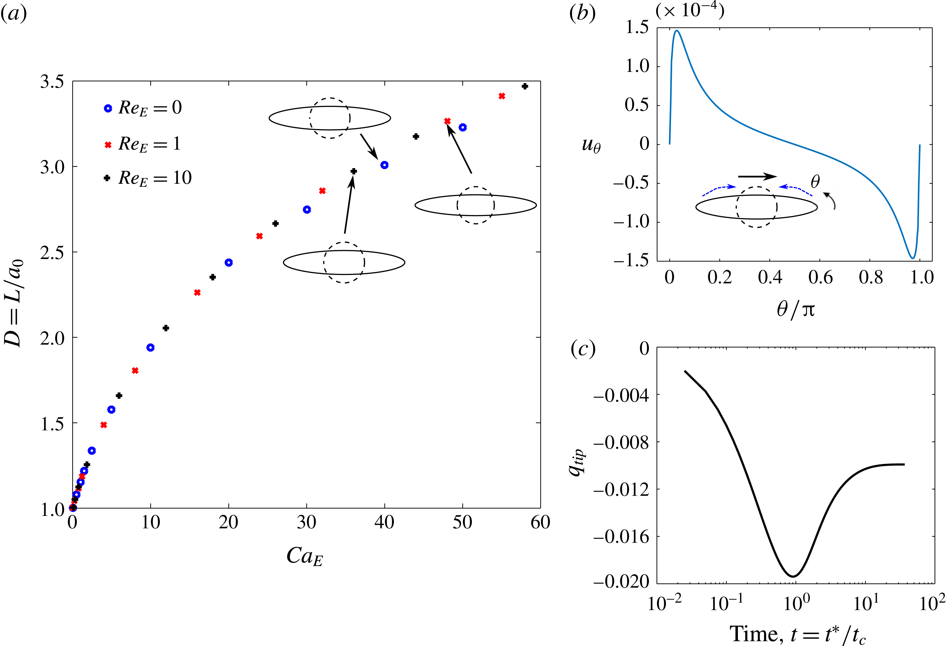
Deformation of a
 $PR_{B}$
drop with
 $(S,R)=(0.03,50)$
. (a) Deformation versus electric capillary number at
 $Re_{E}=0$
(shown by ○),
 $Re_{E}=1$
(shown by
 $\times$
) and
 $Re_{E}=10$
(shown by
 $+$
). The top insets show the steady shape of the drop, and the dashed circle represents the undeformed drop. (b) Dimensionless interfacial tangential velocity,
 $u_{\unicode[STIX]{x1D703}}$
profile at steady state for
 $Ca_{E}=58,Re_{E}=10$
. The inset shows the drop shape at steady state, and the curved lines show the direction of the induced flow. The arrow above the drop shows the direction of the applied electric field. (c) Evolution of dimensionless surface charge density at the tip for
 $Ca_{E}=58,Re_{E}=10$
.

We now consider a second
 $PR_{B}$
drop with
 $M=1$
,
 $S=0.03$
and
 $R=50$
, shown by the square symbol in figure 3. This system is most closely resembled by a drop of squalane doped with 30 pph OLOA, suspended in a 15 wt.% PS solution in DMF. Here, the drop does not break even at the largest capillary numbers tested. The steady prolate shape of the drop is characterized by pointed ends, as shown in figure 12. In this case, surface charge convection increases the final steady deformation of the drop, but it does not induce breakup. The strength of the induced flow is very weak, as seen in the figure. The flow is directed from the poles to the equator, and there are no stagnation points observed. At very high values of
 $Ca_{E}$
, the drop assumes long, stable slender shapes with pointed ends. The evolution of the surface charge density at the poles (figure 12
c) shows that it does not diverge like the drops exhibiting conic cusping, but instead attains a steady value, implying that the conical tips observed for this drop are stable. Slender-body theories for perfect dielectric and leaky dielectric drops in a uniform electric field predict stable drop shapes with conical ends (Stone et al.
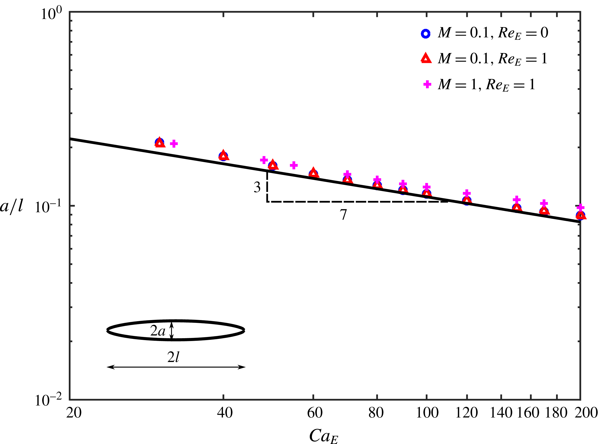
Reference Stone, Lister and Brenner1999; Yariv & Rhodes Reference Yariv and Rhodes2013). These theories predict the slenderness of the drop, defined as the ratio of the equatorial radius of the deformed drop to the half-length of the drop,
 $a/l$
(see inset to figure 13) to scale with the inverse
 $3/7$
-power of
 $Ca_{E}$
, under large applied fields, i.e. for
 $Ca_{E}\gg 1$
. Figure 13 shows the results of our computations at viscosity ratios
 $M=\{0.1,1\}$
, both with and without surface charge convection. All the three results closely obey the scaling
 $a/l\sim Ca_{E}^{-0.4285}$
predicted by the slender-body theories (shown by the black curve). Although the theories have been developed under the assumptions of
 $Re_{E}=0$
and
 $M\ll O(a/l)^{2}$
, it is interesting to note that the computations accounting for surface charge convection and
 $O(1)$
values of the viscosity ratio seem to closely follow the predicted scaling.
Slenderness of the drop as a function of the electric Capillary number for a system with
 $(S,R)=(0.03,50)$
. The symbols correspond to the results of our computations. The black line shows the curve
 $a/l\sim Ca_{E}^{-3/7}$
. The inset shows a deformed drop with pointed tips. The equatorial radius is
 $a$
, and the half-length of the drop is
 $l$
.

In summary, our computations suggest that surface charge convection does not affect the breakup mode of
 $PR_{B}$
drops. In these systems, its role is to increase the final steady deformation of drops. For drops which ultimately break into smaller drops, surface charge convection reduces the time at which the drop undergoes breakup. Drops which deform into long, stable shapes under strong electric fields closely follow slender-body theories, which predict the slenderness to scale as
 $Ca_{E}^{-3/7}$
.
5 Discussion
End pinching and breakup by the formation of pointed ends have both been observed in experiments on drops in electric fields. For highly conducting drops (
 $R<10^{-4}$
) suspended in oils, end pinching has been reported to be the mode of breakup (Allan & Mason Reference Allan and Mason1962; Torza et al.
Reference Torza, Cox and Mason1971; Ha & Yang Reference Ha and Yang2000). For example, a drop of deionized water in castor oil, with
 $(M,S,R)=(1\times 10^{-4},6.3,1\times 10^{-5})$
at
 $Ca_{E}=0.2$
and
 $Re_{E}=0.15$
(Allan & Mason Reference Allan and Mason1962); and a deionized water drop in silicone oil, with
 $(M,S,R)=(0.001,28,1\times 10^{-6})$
at
 $Ca_{E}=0.22$
and
 $Re_{E}=32$
, break via end pinching (Ha & Yang Reference Ha and Yang2000). Breakup via the formation of pointed ends has been observed for soap films (Taylor Reference Taylor1964); sessile water drops exposed to air (Taylor Reference Taylor1969; Gennari et al.
Reference Gennari, Battista, Silva, Grilli, Miccio, Vespini, Coppola, Orlando, Aprin and Slangen2015); sessile water drops suspended in oils (Taylor Reference Taylor1964); leaky dielectric systems and polymer drops (Ha & Yang Reference Ha and Yang2000); and sessile drops of dielectric liquids in air (Gennari et al.
Reference Gennari, Battista, Silva, Grilli, Miccio, Vespini, Coppola, Orlando, Aprin and Slangen2015). In nearly all these studies, the formation of the pointed end, or the conic cusp is followed by the ejection of a very fine jet of fluid, which then disintegrates into drops, whose sizes are orders of magnitude less than the parent drop. While our computations predict the onset of the conic cusp, the transition from the cone to jet is not captured. The transition from cones to fine jets, or the process of ‘electrohydrodynamic tip streaming’ has been resolved computationally for films and drops of leaky dielectric fluids exposed to air (Collins et al.
Reference Collins, Jones, Harris and Basaran2008, Reference Collins, Sambath, Harris and Basaran2013) and electrolytic drops suspended in oils (Pillai et al.
Reference Pillai, Berry, Harvie and Davidson2015, Reference Pillai, Berry, Harvie and Davidson2016). These studies accounted for the surface convection of charges, as well as the transient fluid inertia, by taking finite values of the Ohnesorge number,
 $Oh$
, which is the ratio of capillary to momentum diffusion time scales. The evolution of curvature for a leaky dielectric drop exhibiting tip streaming shows a rapid growth over a very short span of time, akin to conic cusping, which corresponds to the formation of a sharp tip. This is followed by a period of slower growth and then a rapid decline in the curvature due to the transition of the cone into a jet (Collins et al.
Reference Collins, Jones, Harris and Basaran2008). The sharpening of the tip is accompanied by a rapid acceleration of fluid towards the tips, suggesting that accounting for transient fluid inertia, in addition to the convection of charges might be important to capture the cone to jet transition. Our computations account for the surface convection of charges, but not transient fluid inertia, which possibly explains why the evolution of a jet is not observed. There is a sharp transition in the breakup mode of the drop, from disintegration by the formation of lobes to breakup characterized by the formation of cusps at the ends. It will be interesting to understand the mechanism by which the cusps undergo breakup.
From the two
 $PR_{A}$
drops we studied, it is clear that the critical values of
 $Ca_{E}$
and
 $Re_{E}$
at which the transition from end pinching to conic cusping occurs, and the operating space over which each breakup mode is observed, depend on the system being studied, i.e. on the values of
 $M,S$
and
 $R$
. The system shown in figure 9 is predicted to show breakup via the formation of pointed ends over most of the operating space. It is most closely resembled by system ‘NN21’, of a 0.16 cm radius castor oil drop in silicone oil, studied by Ha & Yang (Reference Ha and Yang2000). Their experimental system was reported to have
 $(M,S,R)=(0.874,1.37,0.1)$
and the drop was observed to break with pointed ends at
 $Ca_{E}=1.23$
and
 $Re_{E}=35$
. For these parameters, our computations indeed predict the appearance of pointed ends. In order to move into the region of end pinching for this system, we have to start with drops having
 $a_{0}\sim 10$
cm or higher. It is difficult to apply uniform fields to such large drops in practice; thus for viable drop sizes, this system will show the formation of pointed ends. A castor oil drop suspended in another silicone oil (system ‘NN17’), characterized by
 $(M,S,R)=(0.08,1.37,0.1)$
showed breakup via end pinching at
 $Ca_{E}=1.1$
and
 $Re_{E}=4.3$
(Ha & Yang Reference Ha and Yang2000). Our computations indeed suggest that lowering
 $Ca_{E}$
and
 $Re_{E}$
will shift the breakup mode from pointed ends to end pinching, provided
 $M,S$
and
 $R$
remain constant. Systems ‘NN17’ and ‘NN21’ have the same values of
 $R$
and
 $S$
, however,
 $M$
differs by an order of magnitude. It is here important to recall that we consider a viscosity ratio
 $M=1$
for most of this study. Thus, one expects our results to be relevant to system ‘NN21’
 $(M=0.874)$
. However, the relevance of our results to low viscosity (
 $M\ll 1$
, e.g. system ‘NN17’) or high viscosity drops (
 $M\gg 1$
) is questionable. The viscosity ratio is known to have a great influence on the deformation and breakup of drops in shear and extensional flows (Stone & Leal Reference Stone and Leal1990). Figure 14 shows the result of changing the viscosity of the drop on the deformation and breakup of a prolate A drop. Our computations predict a more viscous drop to deform more before undergoing breakup, and the strength of the interfacial flow to reduce for a more viscous drop, both in agreement with the observations of Lac & Homsy (Reference Lac and Homsy2007); however, the breakup mode remains unchanged. Thus, for a prolate A drop, there is a quantitative change in breakup, but the breakup mode remains the same when there is a moderate change in
 $M$
. The deformation of a prolate B drop was found to be essentially unaffected by the viscosity ratio. For the system with
 $(S,R)=(0.03,50)$
, the deformation changed by 0.5 % when
 $M$
was varied over two decades. It is expected that the boundaries demarcating regions of steady state, end pinching and conic cusping in the
 $Ca_{E}-Re_{E}$
parameter space will change when the viscosity ratio changes, but as figure 14 suggests, a transition will be observed. A detailed study investigating the effect of viscosity ratio on the transition in breakup mode is left as future work.
Effect of viscosity ratio on the deformation and breakup of a prolate A drop. For this system,
 $(S,R)=(1,0.05)$
,
 $Ca_{E}=0.28$
, with (a)
 $Re_{E}=0.05$
and (b)
 $Re_{E}=0.2$
.

Weakly conducting oils like castor oil, silicone oil, squalane and polymers like polystyrene and polyvinylidene fluoride dissolved in suitable solvents have been used to perform experiments on leaky dielectric systems (Allan & Mason Reference Allan and Mason1962; Torza et al.
Reference Torza, Cox and Mason1971; Vizika & Saville Reference Vizika and Saville1992; Ha & Yang Reference Ha and Yang1995, Reference Ha and Yang2000). For these systems, the conductivity and the dielectric constant can be changed to different extents without altering the viscosity by doping with carbon black particles (Yacubowicz & Narkis Reference Yacubowicz and Narkis1986); and the conductivity can be independently changed at constant viscosity and dielectric constant by doping with surfactants (Yezer et al.
Reference Yezer, Khair, Sides and Prieve2015, Reference Yezer, Khair, Sides and Prieve2016). Thus, different regions of the
 $R-S$
parameter space (figure 3) can be accessed with leaky dielectric fluids. However, observing the predicted transition in breakup modes in the same system might be difficult in experiments, because experimentally feasible drop sizes and electric fields will restrict the system to a subset of the
 $Ca_{E}-Re_{E}$
phase space, thus showing one of the breakup modes, instead of a transition between the two modes. A potential way to observe the transition for the same system is to work with higher molecular weight oils, with viscosity of
 $O(10)$
Pa s, or by increasing the conductivity of both the phases by doping with surfactants, leaving the viscosity and dielectric constants relatively unchanged. Increasing the viscosity or the conductivity of the individual phases ensure that the transition occurs at electric fields of
 $O~(\text{kV}~\text{cm}^{-1})$
, with millimetre size drops. Preliminary calculations show that for a drop of polydimethysiloxane (PDMS) in polyisobutylene (PIB), having
 $(M,S,R)=(1,1,0.05)$
, the transition in breakup mode can be observed from end-pinching, with a PDMS drop of initial radius 8 mm, subjected to a field of
 $0.8~\text{kV}~\text{cm}^{-1}$
, to breakup via conical ends with a drop of initial radius
 $80~\unicode[STIX]{x03BC}\text{m}$
, subjected to a field of
 $8~\text{kV}~\text{cm}^{-1}$
. However, the drop would take nearly an hour to break because of the high viscosity of the fluids.
6 Conclusion
We have studied the effect of surface charge convection on the breakup mode of weakly conducting prolate drops, using the boundary integral method. Prolate drops can support two kinds of flows: directed from the equator to the poles of the drop (prolate A,
 $PR_{A}$
drops), and flows from the poles to the equator (prolate B,
 $PR_{B}$
drops). It has been shown that the breakup mode of a prolate A drop changes from end pinching to breakup via conical ends beyond a critical
 $Re_{E}$
. The
 $Ca_{E}-Re_{E}$
parameter space map for two different
 $PR_{A}$
systems (figures 9 and 10) show that the critical parameters at which the transition occurs depend on the system under consideration, i.e. (
 $M,S,R$
) values, however the transition is common to both
 $PR_{A}$
drops. As such, this should be generic to
 $PR_{A}$
drops. Surface charge convection has a less pronounced effect on
 $PR_{B}$
drops. The breakup mode of these drops does not change with increasing
 $Re_{E}$
; however, the final steady deformation increases when charge convection is included. Similar to
 $PR_{A}$
drops, charge convection reduces the critical capillary number for breakup, and the time at which breakup occurs.
Acknowledgements
We are grateful to J. Lanauze for insightful discussions regarding the computations and the results. This work was supported in part by the J. E. Swearingen Graduate Fellowship in Chemical Engineering, Carnegie Mellon University, awarded to R.S.
Appendix. Convergence tests
Here, we present a convergence analysis to select the number of elements,
 $N$
, into which the top half of the drop is partitioned, and the time step size,
 $\unicode[STIX]{x0394}t$
. For this analysis, we select the first
 $PR_{A}$
drop with
 $(M,S,R)=(1,1,0.05)$
at
 $Ca_{E}=0.28$
and
 $Re_{E}=0.15$
. We test three values each for
 $N$
and
 $\unicode[STIX]{x0394}t$
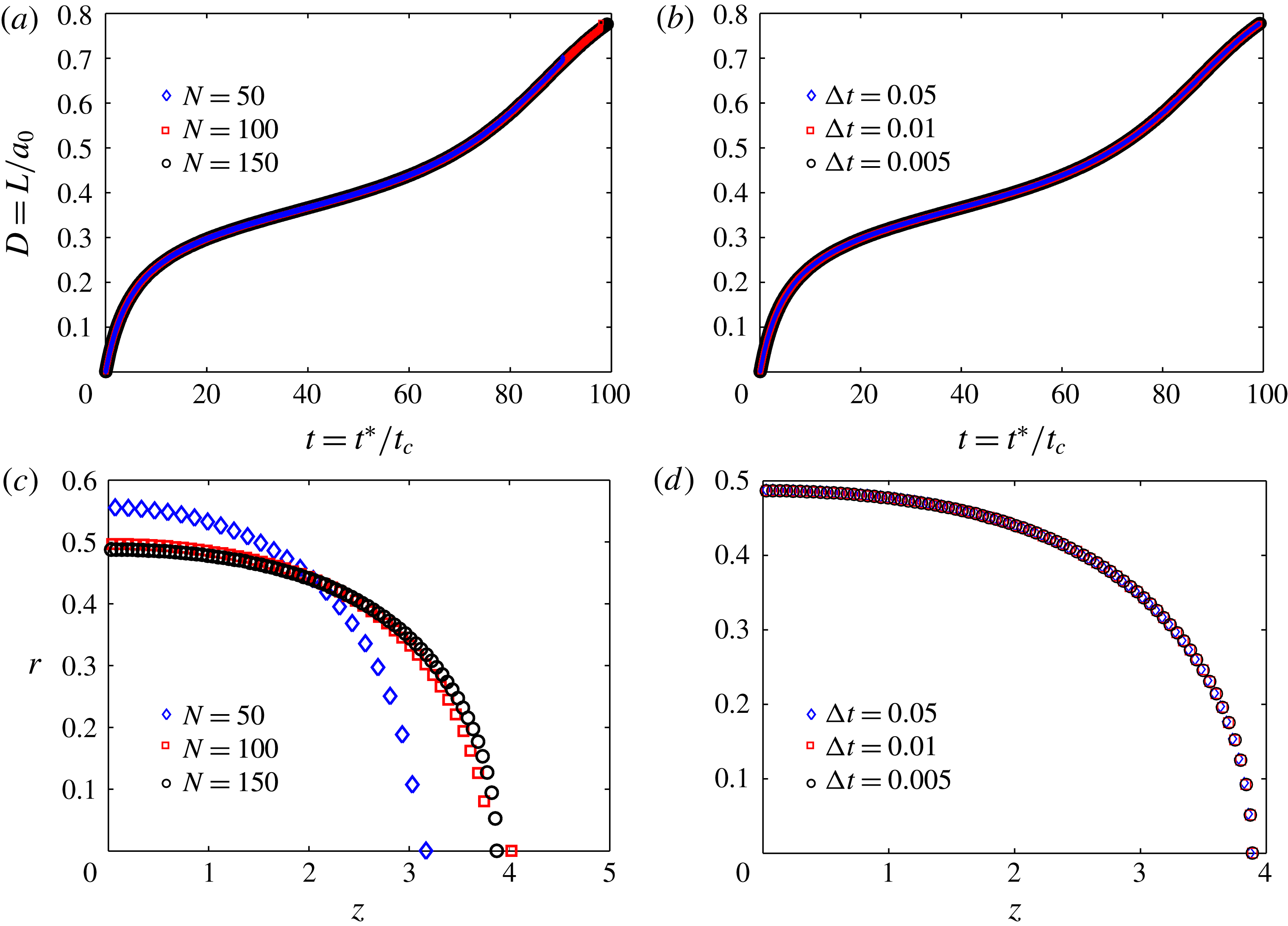
. The results of the computations for the different cases are shown in figure 15. Changing the values of
 $N$
or
 $\unicode[STIX]{x0394}t$
does not significantly alter the result. Moreover, all the values tested predict the formation of conical tips to be the mode of breakup, confirming that this is not a numerical artefact. We fixed
 $N=150$
and
 $\unicode[STIX]{x0394}t=0.05$
in all the computations presented in the main sections of the paper.
Convergence results for a
 $PR_{A}$
drop with
 $(M,S,R)=(1,1,0.05)$
at
 $Ca_{E}=0.28$
and
 $Re_{E}=0.15$
. Deformation of the drop as a function of the dimensionless time for (a) different values of
 $N$
at
 $\unicode[STIX]{x0394}t=0.05$
and (b) different values of
 $\unicode[STIX]{x0394}t$
at
 $N=150$
. Drop shapes before breakup for (c) different values of
 $N$
at
 $\unicode[STIX]{x0394}t=0.05$
and (d) different values of
 $\unicode[STIX]{x0394}t$
at
 $N=150$
.