2 The Kolmogorov and Yaglom equations

In the framework of homogeneous and isotropic turbulence transporting a passive temperature, the Kolmogorov–Obukhov–Corrsin (K41-OC) theory states that, at sufficiently high Reynolds numbers, a range of scales exists where turbulent kinetic energy and temperature variance are only transferred from large to small scales (Kolmogorov Reference Kolmogorov1941b ; Corrsin Reference Corrsin1951; Obukhov Reference Obukhov1968). This exact and non-trivial result can be derived from the equations for the second-order velocity and temperature structure functions $\langle \unicode[STIX]{x1D6FF}u^{2}\rangle =\langle \unicode[STIX]{x1D6FF}u_{i}\unicode[STIX]{x1D6FF}u_{i}\rangle$ and $\langle \unicode[STIX]{x1D6FF}\unicode[STIX]{x1D703}^{2}\rangle =\langle \unicode[STIX]{x1D6FF}\unicode[STIX]{x1D703}\unicode[STIX]{x1D6FF}\unicode[STIX]{x1D703}\rangle$ . Here the angular brackets $\langle \cdot \rangle$ denote the spatial average along the homogeneous directions, and the ensemble average over different configurations, $\unicode[STIX]{x1D6FF}u_{i}=u_{i}(x_{j}+r_{j}/2)-u_{i}(x_{j}-r_{j}/2)$ and $\unicode[STIX]{x1D6FF}\unicode[STIX]{x1D703}=\unicode[STIX]{x1D703}(x_{j}+r_{j}/2)-\unicode[STIX]{x1D703}(x_{j}-r_{j}/2)$ are the fluctuating velocity and temperature increments between the points $x_{j}+r_{j}/2$ and $x_{j}-r_{j}/2$ , and the indices $i,j=1,2,3$ denote the Cartesian components.

Following the heuristic approach proposed by Davidson, Pearson & Staplehurst (Reference Davidson, Pearson and Staplehurst2004), the second-order structure functions $\langle \unicode[STIX]{x1D6FF}u^{2}\rangle$ and $\langle \unicode[STIX]{x1D6FF}\unicode[STIX]{x1D703}^{2}\rangle$ can be interpreted as the turbulent kinetic energy and the temperature variance, respectively, contained by the eddies of length scale smaller than $r=\sqrt{r_{i}r_{i}}$ . Indeed, turbulent scales less than $r$ can actively modulate the signal at $x_{j}+r_{j}/2$ or $x_{j}-r_{j}/2$ but not at both locations simultaneously; thus, they contribute significantly to the structure function. On the other hand, eddies of size much larger than $r$ tend to induce similar signals at both points, with consequent little contribution to the fluctuating increment. In summary, the structure function can be considered along the same line as a high-pass filter, capable of retaining the fluctuations at scales smaller than the filter length $r$ and of damping the information from eddies of size larger than $r$ . Hence, together with the turbulent spectrum, it can be used to study the multiscale features of turbulence (see e.g. Dupuy, Toutant & Bataille Reference Dupuy, Toutant and Bataille2018). In view of this, throughout this paper we will refer to $\langle \unicode[STIX]{x1D6FF}u^{2}\rangle$ and $\langle \unicode[STIX]{x1D6FF}\unicode[STIX]{x1D703}^{2}\rangle$ also as scale energy and scale variance, respectively, adopting the nomenclature introduced by Danaila et al. (Reference Danaila, Anselmet, Zhou and Antonia2001) and employed later by Marati et al. (Reference Marati, Casciola and Piva2004), Cimarelli & De Angelis (Reference Cimarelli and De Angelis2011), Cimarelli, De Angelis & Casciola (Reference Cimarelli, De Angelis and Casciola2013) and Togni, Cimarelli & De Angelis (Reference Togni, Cimarelli and De Angelis2015).

In general, the second-order structure function depends both on the separation vector $r_{j}$ and on the spatial location of the midpoint $x_{j}$ . However, in the case of homogeneous turbulence, the dependence of the scale energy and the scale variance on the midpoint $x_{j}$ drops and, starting from the governing equations, it is possible to derive the following exact equations for $\langle \unicode[STIX]{x1D6FF}u^{2}\rangle$ and $\langle \unicode[STIX]{x1D6FF}\unicode[STIX]{x1D703}^{2}\rangle$ :

(2.1) $$\begin{eqnarray}\displaystyle & \displaystyle -\frac{\unicode[STIX]{x2202}\langle \unicode[STIX]{x1D6FF}u^{2}\unicode[STIX]{x1D6FF}u_{i}\rangle }{\unicode[STIX]{x2202}r_{i}}+2\langle \unicode[STIX]{x1D6FF}f_{i}^{u}\unicode[STIX]{x1D6FF}u_{i}\rangle +2\unicode[STIX]{x1D708}\frac{\unicode[STIX]{x2202}^{2}\langle \unicode[STIX]{x1D6FF}u^{2}\rangle }{\unicode[STIX]{x2202}r_{j}\unicode[STIX]{x2202}r_{j}}-4\langle \unicode[STIX]{x1D716}\rangle =0, & \displaystyle\end{eqnarray}$$

(2.2) $$\begin{eqnarray}\displaystyle & \displaystyle -\frac{\unicode[STIX]{x2202}\langle \unicode[STIX]{x1D6FF}\unicode[STIX]{x1D703}^{2}\unicode[STIX]{x1D6FF}u_{i}\rangle }{\unicode[STIX]{x2202}r_{i}}+2\langle \unicode[STIX]{x1D6FF}f_{i}^{\unicode[STIX]{x1D703}}\unicode[STIX]{x1D6FF}u_{i}\rangle +2\unicode[STIX]{x1D705}\frac{\unicode[STIX]{x2202}^{2}\langle \unicode[STIX]{x1D6FF}\unicode[STIX]{x1D703}^{2}\rangle }{\unicode[STIX]{x2202}r_{j}\unicode[STIX]{x2202}r_{j}}-2\langle \unicode[STIX]{x1D712}\rangle =0, & \displaystyle\end{eqnarray}$$

where $\unicode[STIX]{x1D708}$ is the kinematic viscosity, $\unicode[STIX]{x1D705}$ is the thermal diffusivity, $\unicode[STIX]{x1D716}=2\unicode[STIX]{x1D708}(S_{ij}S_{ij})$ is the dissipation of turbulent kinetic energy, $S_{ij}=0.5(\unicode[STIX]{x2202}u_{i}/\unicode[STIX]{x2202}x_{j}+\unicode[STIX]{x2202}u_{j}/\unicode[STIX]{x2202}x_{i})$ is the fluctuating strain-rate tensor, $\unicode[STIX]{x1D712}=2\unicode[STIX]{x1D705}(\unicode[STIX]{x2202}\unicode[STIX]{x1D703}/\unicode[STIX]{x2202}x_{i})(\unicode[STIX]{x2202}\unicode[STIX]{x1D703}/\unicode[STIX]{x2202}x_{i})$ is the dissipation of temperature variance, and $2\langle \unicode[STIX]{x1D6FF}f_{i}^{u}\unicode[STIX]{x1D6FF}u_{i}\rangle$ and $2\langle \unicode[STIX]{x1D6FF}f_{i}^{\unicode[STIX]{x1D703}}\unicode[STIX]{x1D6FF}u_{i}\rangle$ are the homogeneous source terms due to the external forcing $f_{i}^{u}$ and $f_{i}^{\unicode[STIX]{x1D703}}$ active at large scales. The first term in (2.1) and (2.2) denotes the rate at which scales smaller than $r$ receive (release) turbulent kinetic energy and temperature variance from (to) larger ones via inertial mechanisms, whereas the third term in (2.1) and (2.2) is indicative of the amount of turbulent kinetic energy and temperature variance diffused in the space of scales. In the case of high-intensity turbulent flows, an inertial range is supposed to develop for $\unicode[STIX]{x1D702}_{k},\unicode[STIX]{x1D702}_{b}\ll r\ll \ell _{0}$ , where $\unicode[STIX]{x1D702}_{k}$ , $\unicode[STIX]{x1D702}_{b}$ and $\ell _{0}$ are the Kolmogorov, the Batchelor and the integral scales, respectively. Both production and viscous diffusion effects are negligible within this range, thus (2.1) and (2.2) reduce to

(2.3) $$\begin{eqnarray}\displaystyle & \displaystyle \frac{\unicode[STIX]{x2202}\langle \unicode[STIX]{x1D6FF}u^{2}\unicode[STIX]{x1D6FF}u_{i}\rangle }{\unicode[STIX]{x2202}r_{i}}=-4\langle \unicode[STIX]{x1D716}\rangle , & \displaystyle\end{eqnarray}$$

(2.4) $$\begin{eqnarray}\displaystyle & \displaystyle \frac{\unicode[STIX]{x2202}\langle \unicode[STIX]{x1D6FF}\unicode[STIX]{x1D703}^{2}\unicode[STIX]{x1D6FF}u_{i}\rangle }{\unicode[STIX]{x2202}r_{i}}=-2\langle \unicode[STIX]{x1D712}\rangle , & \displaystyle\end{eqnarray}$$

stating that the amount of turbulent kinetic energy and temperature variance transferred per unit time to scales less than $r$ is equal to the average dissipation rates. It should be pointed out that (2.3) and (2.4) further simplify to the familiar four-fifths and four-thirds laws, respectively, if turbulence is assumed to be also isotropic.

Figure 1.

Sketch of the Rayleigh–Bénard convection set-up.

The fundamental aspect of actual turbulent flows is the presence of a cycle along which fluctuations are generated, transported among different scales and space locations, and finally dissipated. Inhomogeneity modifies the scale-by-scale budgets (2.1) and (2.2) by introducing an autonomous production, a transport in physical space and by spatially modulating the balances. Fully developed turbulence in laterally unbounded RBC is statistically inhomogeneous in the wall-normal direction but homogeneous and isotropic in the wall-parallel planes. We exploit these symmetries, and in particular the isotropy in the wall-parallel planes, by considering a cylindrical coordinate system $(\unicode[STIX]{x1D70C},\unicode[STIX]{x1D719},z)$ rather than a Cartesian one $(x,y,z)$ ; see the sketch in figure 1. The wall-parallel coordinates are $x=x_{1}$ and $y=x_{2}$ while the wall-normal coordinate, $z=x_{3}$ , is zero at the lower wall. The cylindrical coordinates are defined such that $\unicode[STIX]{x1D70C}=\sqrt{x^{2}+y^{2}}$ and $\unicode[STIX]{x1D719}=\arctan (y/x)$ . The scale-by-scale budgets for RBC can be derived starting from the continuity, momentum and energy equations under the Boussinesq approximation (Hill Reference Hill2002) and, for a cylindrical coordinate system, result in

(2.5) $$\begin{eqnarray}\displaystyle & & \displaystyle \displaystyle -\frac{\unicode[STIX]{x2202}\langle w^{\dagger }\unicode[STIX]{x1D6FF}u^{2}\rangle }{\unicode[STIX]{x2202}z}-2\frac{\unicode[STIX]{x2202}\langle \unicode[STIX]{x1D6FF}p\unicode[STIX]{x1D6FF}w\rangle }{\unicode[STIX]{x2202}z}+\frac{\unicode[STIX]{x1D708}}{2}\frac{\unicode[STIX]{x2202}^{2}\langle \unicode[STIX]{x1D6FF}u^{2}\rangle }{\unicode[STIX]{x2202}z^{2}}-\frac{1}{r_{\unicode[STIX]{x1D70C}}}\frac{\unicode[STIX]{x2202}}{\unicode[STIX]{x2202}r_{\unicode[STIX]{x1D70C}}}(r_{\unicode[STIX]{x1D70C}}\langle \unicode[STIX]{x1D6FF}u^{2}\unicode[STIX]{x1D6FF}u_{\unicode[STIX]{x1D70C}}\rangle )\nonumber\\ \displaystyle & & \displaystyle \quad \displaystyle -\,\frac{\unicode[STIX]{x2202}\langle \unicode[STIX]{x1D6FF}u^{2}\unicode[STIX]{x1D6FF}w\rangle }{\unicode[STIX]{x2202}r_{z}}+2\unicode[STIX]{x1D6FC}g\langle \unicode[STIX]{x1D6FF}\unicode[STIX]{x1D703}\unicode[STIX]{x1D6FF}w\rangle +\frac{2\unicode[STIX]{x1D708}}{r_{\unicode[STIX]{x1D70C}}}\frac{\unicode[STIX]{x2202}}{\unicode[STIX]{x2202}r_{\unicode[STIX]{x1D70C}}}\left(r_{\unicode[STIX]{x1D70C}}\frac{\unicode[STIX]{x2202}\langle \unicode[STIX]{x1D6FF}u^{2}\rangle }{\unicode[STIX]{x2202}r_{\unicode[STIX]{x1D70C}}}\right)+2\unicode[STIX]{x1D708}\frac{\unicode[STIX]{x2202}^{2}\langle \unicode[STIX]{x1D6FF}u^{2}\rangle }{\unicode[STIX]{x2202}r_{z}^{2}}-4\langle \tilde{\unicode[STIX]{x1D716}}^{\dagger }\rangle =0\qquad\end{eqnarray}$$

and

(2.6) $$\begin{eqnarray}\displaystyle & & \displaystyle \displaystyle -\frac{\unicode[STIX]{x2202}\langle w^{\dagger }\unicode[STIX]{x1D6FF}\unicode[STIX]{x1D703}^{2}\rangle }{\unicode[STIX]{x2202}z}+\frac{\unicode[STIX]{x1D705}}{2}\frac{\unicode[STIX]{x2202}^{2}\langle \unicode[STIX]{x1D6FF}\unicode[STIX]{x1D703}^{2}\rangle }{\unicode[STIX]{x2202}z^{2}}-\frac{1}{r_{\unicode[STIX]{x1D70C}}}\frac{\unicode[STIX]{x2202}}{\unicode[STIX]{x2202}r_{\unicode[STIX]{x1D70C}}}(r_{\unicode[STIX]{x1D70C}}\langle \unicode[STIX]{x1D6FF}\unicode[STIX]{x1D703}^{2}\unicode[STIX]{x1D6FF}u_{\unicode[STIX]{x1D70C}}\rangle )-\frac{\unicode[STIX]{x2202}\langle \unicode[STIX]{x1D6FF}\unicode[STIX]{x1D703}^{2}\unicode[STIX]{x1D6FF}w\rangle }{\unicode[STIX]{x2202}r_{z}}\nonumber\\ \displaystyle & & \displaystyle \quad \displaystyle -\,2\langle w^{\dagger }\unicode[STIX]{x1D6FF}\unicode[STIX]{x1D703}\rangle \frac{\unicode[STIX]{x2202}\unicode[STIX]{x1D6FF}\unicode[STIX]{x1D6E9}}{\unicode[STIX]{x2202}z}-2\langle \unicode[STIX]{x1D6FF}w\unicode[STIX]{x1D6FF}\unicode[STIX]{x1D703}\rangle \left(\frac{\text{d}\unicode[STIX]{x1D6E9}}{\text{d}z}\right)^{\dagger }+\frac{2\unicode[STIX]{x1D705}}{r_{\unicode[STIX]{x1D70C}}}\frac{\unicode[STIX]{x2202}}{\unicode[STIX]{x2202}r_{\unicode[STIX]{x1D70C}}}\left(r_{\unicode[STIX]{x1D70C}}\frac{\unicode[STIX]{x2202}\langle \unicode[STIX]{x1D6FF}\unicode[STIX]{x1D703}^{2}\rangle }{\unicode[STIX]{x2202}r_{\unicode[STIX]{x1D70C}}}\right)+2\unicode[STIX]{x1D705}\frac{\unicode[STIX]{x2202}^{2}\langle \unicode[STIX]{x1D6FF}\unicode[STIX]{x1D703}^{2}\rangle }{\unicode[STIX]{x2202}r_{z}^{2}}\quad \nonumber\\ \displaystyle & & \displaystyle \quad \displaystyle -\,2\langle \unicode[STIX]{x1D712}^{\dagger }\rangle =0,\end{eqnarray}$$

where $g$ is the gravity acceleration, $\unicode[STIX]{x1D6FC}$ is the thermal expansion coefficient and $\tilde{\unicode[STIX]{x1D716}}=\unicode[STIX]{x1D708}(\unicode[STIX]{x2202}u_{i}/\unicode[STIX]{x2202}x_{j})(\unicode[STIX]{x2202}u_{i}/\unicode[STIX]{x2202}x_{j})$ is the pseudo-dissipation of turbulent kinetic energy. The dagger $\dagger$ denotes the midpoint average, $\unicode[STIX]{x1D6FD}^{\dagger }=(\unicode[STIX]{x1D6FD}(x_{j}-r_{j}/2)+\unicode[STIX]{x1D6FD}(x_{j}+r_{j}/2))/2$ for the generic quantity $\unicode[STIX]{x1D6FD}$ . The radial, the circumferential and the vertical components of the separation vector are $r_{\unicode[STIX]{x1D70C}}$ , $r_{\unicode[STIX]{x1D719}}$ and $r_{z}$ , whereas the same components of the velocity structure function are $\unicode[STIX]{x1D6FF}u_{\unicode[STIX]{x1D70C}}$ , $\unicode[STIX]{x1D6FF}u_{\unicode[STIX]{x1D719}}$ and $\unicode[STIX]{x1D6FF}w$ . Let us note that all the $r_{\unicode[STIX]{x1D719}}$ -derivative terms arising from the formulation in cylindrical coordinates are zero for statistical isotropy while, for statistical homogeneity, also the $\unicode[STIX]{x1D719}$ - and $\unicode[STIX]{x1D70C}$ -derivatives are null.

An additional class of terms, namely the ones with the $z$ -derivative, appear in the inhomogeneous case, denoting the amount of scale energy and scale variance received (released) from (to) other wall distances. Moreover, $2\unicode[STIX]{x1D6FC}g\langle \unicode[STIX]{x1D6FF}\unicode[STIX]{x1D703}\unicode[STIX]{x1D6FF}w\rangle$ and $-2\langle w^{\dagger }\unicode[STIX]{x1D6FF}\unicode[STIX]{x1D703}\rangle (\unicode[STIX]{x2202}\unicode[STIX]{x1D6FF}\unicode[STIX]{x1D6E9}/\unicode[STIX]{x2202}z)-2\langle \unicode[STIX]{x1D6FF}w\unicode[STIX]{x1D6FF}\unicode[STIX]{x1D703}\rangle (\text{d}\unicode[STIX]{x1D6E9}/\text{d}z)^{\dagger }$ are the inhomogeneous production terms, where $\unicode[STIX]{x1D6E9}$ is the mean temperature. At sufficiently high Reynolds numbers, an inertial range of scales is assumed to exist in which turbulence is locally homogeneous and isotropic, viscous effects are negligible, and temperature acts as a passive scalar (Lohse & Xia Reference Lohse and Xia2010). In this case, it is easy to demonstrate that (2.5) and (2.6) simplify to (2.3) and (2.4) and, with further manipulations, to the four-fifths and four-thirds laws, respectively.

Equations (2.5) and (2.6), written in the complete three-dimensional $(r_{\unicode[STIX]{x1D70C}},r_{z},z)$ space, are the Kolmogorov and Yaglom equations for RBC. The Kolmogorov equation for an axisymmetric flow has already been proposed by Danaila et al. (Reference Danaila, Krawczynski, Thiesset and Renou2012), while the Yaglom equation has been extended before only to homogeneous anisotropic turbulence (Gauding et al. Reference Gauding, Wick, Pitsch and Peters2014). For the sake of simplicity, we restrict the following analysis to the reduced $(r_{\unicode[STIX]{x1D70C}},z)$ space, where $r_{z}=0$ (Cimarelli et al. Reference Cimarelli, De Angelis, Jiménez and Casciola2016). The reduced scale-by-scale budgets are non-dimensionalized using $H$ , $\unicode[STIX]{x0394}\unicode[STIX]{x1D6E9}=\unicode[STIX]{x1D6E9}_{1}-\unicode[STIX]{x1D6E9}_{2}$ and $U_{f}=\sqrt{g\unicode[STIX]{x1D6FC}\unicode[STIX]{x0394}\unicode[STIX]{x1D6E9}H}$ as characteristic length, temperature and velocity scales, where $H$ is the height of the fluid layer, $\unicode[STIX]{x1D6E9}_{1}$ and $\unicode[STIX]{x1D6E9}_{2}$ are the temperature of the lower and upper walls, respectively, and $U_{f}$ is the free-fall velocity. The resulting equations, hereafter referred to as reduced Kolmogorov and Yaglom equations, can be written in a compact form, i.e.

(2.7) $$\begin{eqnarray}\displaystyle & \displaystyle T_{c}^{u}+I_{r}^{u}+\unicode[STIX]{x1D6F1}^{u}+E_{e}^{u}=0, & \displaystyle\end{eqnarray}$$

(2.8) $$\begin{eqnarray}\displaystyle & \displaystyle T_{c}^{\unicode[STIX]{x1D703}}+I_{r}^{\unicode[STIX]{x1D703}}+\unicode[STIX]{x1D6F1}^{\unicode[STIX]{x1D703}}+E_{e}^{\unicode[STIX]{x1D703}}=0, & \displaystyle\end{eqnarray}$$

where $T_{c}^{u}=I_{c}^{u}+P+D_{c}^{u}$ and $T_{c}^{\unicode[STIX]{x1D703}}=I_{c}^{\unicode[STIX]{x1D703}}+D_{c}^{\unicode[STIX]{x1D703}}$ represent the sum of the transport terms in physical space and hence will be hereafter called the overall transports. On the other hand, $E_{e}^{u}=D_{r}^{u}+E^{u}$ and $E_{e}^{\unicode[STIX]{x1D703}}=D_{r}^{\unicode[STIX]{x1D703}}+E^{\unicode[STIX]{x1D703}}$ represent the overall effect of viscosity on transporting scale energy and scale variance to the smallest scales of the flow by $D_{r}^{u}$ and $D_{r}^{\unicode[STIX]{x1D703}}$ , where they are finally dissipated by $E^{u}$ and $E^{\unicode[STIX]{x1D703}}$ . Accordingly, $E_{e}^{u}$ and $E_{e}^{\unicode[STIX]{x1D703}}$ will be hereafter called effective dissipations. The different contributions to the overall transports and to the effective dissipations are, in order,

(2.9) $$\begin{eqnarray}\left.\begin{array}{@{}c@{}}\displaystyle I_{c}^{u}=-\frac{\unicode[STIX]{x2202}\langle w^{\dagger }\unicode[STIX]{x1D6FF}u^{2}\rangle }{\unicode[STIX]{x2202}z},\quad P=-2\frac{\unicode[STIX]{x2202}\langle \unicode[STIX]{x1D6FF}p\unicode[STIX]{x1D6FF}w\rangle }{\unicode[STIX]{x2202}z},\quad D_{c}^{u}=\frac{1}{2}\sqrt{\frac{Pr}{Ra}}\frac{\unicode[STIX]{x2202}^{2}\langle \unicode[STIX]{x1D6FF}u^{2}\rangle }{\unicode[STIX]{x2202}z^{2}},\\ \displaystyle I_{c}^{\unicode[STIX]{x1D703}}=-\frac{\unicode[STIX]{x2202}\langle w^{\dagger }\unicode[STIX]{x1D6FF}\unicode[STIX]{x1D703}^{2}\rangle }{\unicode[STIX]{x2202}z},\quad D_{c}^{\unicode[STIX]{x1D703}}=\frac{1}{2\sqrt{PrRa}}\frac{\unicode[STIX]{x2202}^{2}\langle \unicode[STIX]{x1D6FF}\unicode[STIX]{x1D703}^{2}\rangle }{\unicode[STIX]{x2202}z^{2}},\end{array}\right\}\end{eqnarray}$$

and

(2.10) $$\begin{eqnarray}\displaystyle \left.\begin{array}{@{}c@{}}\displaystyle D_{r}^{u}=2\sqrt{\frac{Pr}{Ra}}\frac{1}{r_{\unicode[STIX]{x1D70C}}}\frac{\unicode[STIX]{x2202}}{\unicode[STIX]{x2202}r_{\unicode[STIX]{x1D70C}}}\left(r_{\unicode[STIX]{x1D70C}}\frac{\unicode[STIX]{x2202}\langle \unicode[STIX]{x1D6FF}u^{2}\rangle }{\unicode[STIX]{x2202}r_{\unicode[STIX]{x1D70C}}}\right)+2\sqrt{\frac{Pr}{Ra}}\frac{\unicode[STIX]{x2202}^{2}\langle \unicode[STIX]{x1D6FF}u^{2}\rangle }{\unicode[STIX]{x2202}r_{z}^{2}}\bigg|_{\substack{ r_{z}=0}},\quad E^{u}=-4\langle \tilde{\unicode[STIX]{x1D716}}\rangle ,\\ \displaystyle \displaystyle D_{r}^{\unicode[STIX]{x1D703}}=\frac{2}{\sqrt{PrRa}}\frac{1}{r_{\unicode[STIX]{x1D70C}}}\frac{\unicode[STIX]{x2202}}{\unicode[STIX]{x2202}r_{\unicode[STIX]{x1D70C}}}\left(r_{\unicode[STIX]{x1D70C}}\frac{\unicode[STIX]{x2202}\langle \unicode[STIX]{x1D6FF}\unicode[STIX]{x1D703}^{2}\rangle }{\unicode[STIX]{x2202}r_{\unicode[STIX]{x1D70C}}}\right)+\frac{2}{\sqrt{PrRa}}\frac{\unicode[STIX]{x2202}^{2}\langle \unicode[STIX]{x1D6FF}\unicode[STIX]{x1D703}^{2}\rangle }{\unicode[STIX]{x2202}r_{z}^{2}}\bigg|_{\substack{ r_{z}=0}},\quad E^{\unicode[STIX]{x1D703}}=-2\langle \unicode[STIX]{x1D712}\rangle ,\end{array}\right\} & & \displaystyle\end{eqnarray}$$

while the transports in the space of scales and the production terms are

(2.11) $$\begin{eqnarray}\left.\begin{array}{@{}c@{}}\displaystyle I_{r}^{u}=-\frac{1}{r_{\unicode[STIX]{x1D70C}}}\frac{\unicode[STIX]{x2202}}{\unicode[STIX]{x2202}r_{\unicode[STIX]{x1D70C}}}(r_{\unicode[STIX]{x1D70C}}\langle \unicode[STIX]{x1D6FF}u^{2}\unicode[STIX]{x1D6FF}u_{\unicode[STIX]{x1D70C}}\rangle )-\frac{\unicode[STIX]{x2202}\langle \unicode[STIX]{x1D6FF}u^{2}\unicode[STIX]{x1D6FF}w\rangle }{\unicode[STIX]{x2202}r_{z}}\bigg|_{\substack{ r_{z}=0}},\quad \unicode[STIX]{x1D6F1}^{u}=2\langle \unicode[STIX]{x1D6FF}\unicode[STIX]{x1D703}\unicode[STIX]{x1D6FF}w\rangle ,\\ \displaystyle I_{r}^{\unicode[STIX]{x1D703}}=-\frac{1}{r_{\unicode[STIX]{x1D70C}}}\frac{\unicode[STIX]{x2202}}{\unicode[STIX]{x2202}r_{\unicode[STIX]{x1D70C}}}(r_{\unicode[STIX]{x1D70C}}\langle \unicode[STIX]{x1D6FF}\unicode[STIX]{x1D703}^{2}\unicode[STIX]{x1D6FF}u_{\unicode[STIX]{x1D70C}}\rangle )-\frac{\unicode[STIX]{x2202}\langle \unicode[STIX]{x1D6FF}\unicode[STIX]{x1D703}^{2}\unicode[STIX]{x1D6FF}w\rangle }{\unicode[STIX]{x2202}r_{z}}\bigg|_{\substack{ r_{z}=0}},\quad \unicode[STIX]{x1D6F1}^{\unicode[STIX]{x1D703}}=-2\langle \unicode[STIX]{x1D6FF}w\unicode[STIX]{x1D6FF}\unicode[STIX]{x1D703}\rangle \frac{\text{d}\unicode[STIX]{x1D6E9}}{\text{d}z}.\end{array}\right\}\end{eqnarray}$$

It must be pointed out that the contribution of the term $-2\langle w^{\dagger }\unicode[STIX]{x1D6FF}\unicode[STIX]{x1D703}\rangle (\unicode[STIX]{x2202}\unicode[STIX]{x1D6FF}\unicode[STIX]{x1D6E9}/\unicode[STIX]{x2202}z)$ to the production of scale variance vanishes, since $\unicode[STIX]{x1D6FF}\unicode[STIX]{x1D6E9}=0$ for $r_{z}=0$ . Finally, the non-dimensional groups appearing are the Rayleigh number, $Ra=g\unicode[STIX]{x1D6FC}\unicode[STIX]{x0394}\unicode[STIX]{x1D6E9}H^{3}/\unicode[STIX]{x1D708}\unicode[STIX]{x1D705}$ , and the Prandtl number, $Pr=\unicode[STIX]{x1D708}/\unicode[STIX]{x1D705}$ .

Let us extend the Kolmogorov and Yaglom equations to filtered velocity and temperature fields. Starting from the filtered continuity, momentum and energy equations under the Boussinesq approximation and by following the same procedure used to derive (2.5) and (2.6) (Hill Reference Hill2002), it is possible to obtain the budgets of resolved scale energy $\langle \unicode[STIX]{x1D6FF}\bar{u}^{2}\rangle =\langle \unicode[STIX]{x1D6FF}\bar{u}_{i}\unicode[STIX]{x1D6FF}\bar{u}_{i}\rangle$ and resolved scale variance $\langle \unicode[STIX]{x1D6FF}\bar{\unicode[STIX]{x1D703}}^{2}\rangle =\langle \unicode[STIX]{x1D6FF}\bar{\unicode[STIX]{x1D703}}\unicode[STIX]{x1D6FF}\bar{\unicode[STIX]{x1D703}}\rangle$ :

(2.12) $$\begin{eqnarray}\displaystyle & & \displaystyle \displaystyle -\frac{\unicode[STIX]{x2202}\langle \bar{w}^{\dagger }\unicode[STIX]{x1D6FF}\bar{u}^{2}\rangle }{\unicode[STIX]{x2202}z}-2\frac{\unicode[STIX]{x2202}\langle \unicode[STIX]{x1D6FF}\bar{p}\unicode[STIX]{x1D6FF}\bar{w}\rangle }{\unicode[STIX]{x2202}z}+\frac{\unicode[STIX]{x1D708}}{2}\frac{\unicode[STIX]{x2202}^{2}\langle \unicode[STIX]{x1D6FF}\bar{u}^{2}\rangle }{\unicode[STIX]{x2202}z^{2}}-\frac{1}{r_{\unicode[STIX]{x1D70C}}}\frac{\unicode[STIX]{x2202}}{\unicode[STIX]{x2202}r_{\unicode[STIX]{x1D70C}}}(r_{\unicode[STIX]{x1D70C}}\langle \unicode[STIX]{x1D6FF}\bar{u}^{2}\unicode[STIX]{x1D6FF}\bar{u}_{\unicode[STIX]{x1D70C}}\rangle )\nonumber\\ \displaystyle & & \displaystyle \quad \displaystyle -\,\frac{\unicode[STIX]{x2202}\langle \unicode[STIX]{x1D6FF}\bar{u}^{2}\unicode[STIX]{x1D6FF}\bar{w}\rangle }{\unicode[STIX]{x2202}r_{z}}+2\unicode[STIX]{x1D6FC}g\langle \unicode[STIX]{x1D6FF}\bar{\unicode[STIX]{x1D703}}\unicode[STIX]{x1D6FF}\bar{w}\rangle +\frac{2\unicode[STIX]{x1D708}}{r_{\unicode[STIX]{x1D70C}}}\frac{\unicode[STIX]{x2202}}{\unicode[STIX]{x2202}r_{\unicode[STIX]{x1D70C}}}\left(r_{\unicode[STIX]{x1D70C}}\frac{\unicode[STIX]{x2202}\langle \unicode[STIX]{x1D6FF}\bar{u}^{2}\rangle }{\unicode[STIX]{x2202}r_{\unicode[STIX]{x1D70C}}}\right)+2\unicode[STIX]{x1D708}\frac{\unicode[STIX]{x2202}^{2}\langle \unicode[STIX]{x1D6FF}\bar{u}^{2}\rangle }{\unicode[STIX]{x2202}r_{z}^{2}}-4\langle \bar{\tilde{\unicode[STIX]{x1D716}}}^{\dagger }\rangle \quad \nonumber\\ \displaystyle & & \displaystyle \quad \displaystyle -\,\frac{\unicode[STIX]{x2202}\langle \unicode[STIX]{x1D6FF}\unicode[STIX]{x1D70F}_{i3}\unicode[STIX]{x1D6FF}\bar{u}_{i}\rangle }{\unicode[STIX]{x2202}z}-\frac{4}{r_{\unicode[STIX]{x1D70C}}}\frac{\unicode[STIX]{x2202}}{\unicode[STIX]{x2202}r_{\unicode[STIX]{x1D70C}}}(r_{\unicode[STIX]{x1D70C}}\langle \unicode[STIX]{x1D70F}_{ij}^{\dagger }\unicode[STIX]{x1D6FF}\bar{u}_{i}\hat{\unicode[STIX]{x1D70C}}_{j}\rangle )-4\frac{\unicode[STIX]{x2202}\langle \unicode[STIX]{x1D70F}_{i3}^{\dagger }\unicode[STIX]{x1D6FF}\bar{u}_{i}\rangle }{\unicode[STIX]{x2202}r_{z}}\bigg|_{\substack{ r_{z}=0}}-4\langle \unicode[STIX]{x1D716}_{sgs}\rangle =0\end{eqnarray}$$

and

(2.13) $$\begin{eqnarray}\displaystyle & & \displaystyle \displaystyle -\frac{\unicode[STIX]{x2202}\langle \bar{w}^{\dagger }\unicode[STIX]{x1D6FF}\bar{\unicode[STIX]{x1D703}}^{2}\rangle }{\unicode[STIX]{x2202}z}+\frac{\unicode[STIX]{x1D705}}{2}\frac{\unicode[STIX]{x2202}^{2}\langle \unicode[STIX]{x1D6FF}\bar{\unicode[STIX]{x1D703}}^{2}\rangle }{\unicode[STIX]{x2202}z^{2}}-\frac{1}{r_{\unicode[STIX]{x1D70C}}}\frac{\unicode[STIX]{x2202}}{\unicode[STIX]{x2202}r_{\unicode[STIX]{x1D70C}}}(r_{\unicode[STIX]{x1D70C}}\langle \unicode[STIX]{x1D6FF}\bar{\unicode[STIX]{x1D703}}^{2}\unicode[STIX]{x1D6FF}\bar{u}_{\unicode[STIX]{x1D70C}}\rangle )-\frac{\unicode[STIX]{x2202}\langle \unicode[STIX]{x1D6FF}\bar{\unicode[STIX]{x1D703}}^{2}\unicode[STIX]{x1D6FF}\bar{w}\rangle }{\unicode[STIX]{x2202}r_{z}}\nonumber\\ \displaystyle & & \displaystyle \quad \displaystyle -\,2\langle \bar{w}^{\dagger }\unicode[STIX]{x1D6FF}\bar{\unicode[STIX]{x1D703}}\rangle \frac{\unicode[STIX]{x2202}\unicode[STIX]{x1D6FF}\bar{\unicode[STIX]{x1D6E9}}}{\unicode[STIX]{x2202}z}-2\langle \unicode[STIX]{x1D6FF}\bar{w}\unicode[STIX]{x1D6FF}\bar{\unicode[STIX]{x1D703}}\rangle \left(\frac{\text{d}\bar{\unicode[STIX]{x1D6E9}}}{\text{d}z}\right)^{\dagger }+\frac{2\unicode[STIX]{x1D705}}{r_{\unicode[STIX]{x1D70C}}}\frac{\unicode[STIX]{x2202}}{\unicode[STIX]{x2202}r_{\unicode[STIX]{x1D70C}}}\left(r_{\unicode[STIX]{x1D70C}}\frac{\unicode[STIX]{x2202}\langle \unicode[STIX]{x1D6FF}\bar{\unicode[STIX]{x1D703}}^{2}\rangle }{\unicode[STIX]{x2202}r_{\unicode[STIX]{x1D70C}}}\right)+2\unicode[STIX]{x1D705}\frac{\unicode[STIX]{x2202}^{2}\langle \unicode[STIX]{x1D6FF}\bar{\unicode[STIX]{x1D703}}^{2}\rangle }{\unicode[STIX]{x2202}r_{z}^{2}}\quad \nonumber\\ \displaystyle & & \displaystyle \quad \displaystyle -\,2\langle \bar{\unicode[STIX]{x1D712}}^{\dagger }\rangle -\frac{\unicode[STIX]{x2202}\langle \unicode[STIX]{x1D6FF}q_{z}\unicode[STIX]{x1D6FF}\bar{\unicode[STIX]{x1D703}}\rangle }{\unicode[STIX]{x2202}z}-\frac{4}{r_{\unicode[STIX]{x1D70C}}}\frac{\unicode[STIX]{x2202}}{\unicode[STIX]{x2202}r_{\unicode[STIX]{x1D70C}}}(r_{\unicode[STIX]{x1D70C}}\langle q_{\unicode[STIX]{x1D70C}}^{\dagger }\unicode[STIX]{x1D6FF}\bar{\unicode[STIX]{x1D703}}\rangle )-4\frac{\unicode[STIX]{x2202}\langle q_{z}^{\dagger }\unicode[STIX]{x1D6FF}\bar{\unicode[STIX]{x1D703}}\rangle }{\unicode[STIX]{x2202}r_{z}}\bigg|_{\substack{ r_{z}=0}}-2\langle \unicode[STIX]{x1D712}_{sgs}\rangle =0.\end{eqnarray}$$

Equations (2.12) and (2.13) share several types of terms with the corresponding unfiltered equations (2.5) and (2.6) which can be better highlighted by considering the filtered reduced Kolmogorov and Yaglom equations,

(2.14) $$\begin{eqnarray}\displaystyle & \displaystyle \bar{T}_{c}^{u}+\bar{I}_{r}^{u}+\bar{\unicode[STIX]{x1D6F1}}^{u}+\bar{E}_{e}^{u}+T_{c,sgs}^{u}+T_{r,sgs}^{u}+E_{sgs}^{u}=0, & \displaystyle\end{eqnarray}$$

(2.15) $$\begin{eqnarray}\displaystyle & \displaystyle \bar{T}_{c}^{\unicode[STIX]{x1D703}}+\bar{I}_{r}^{\unicode[STIX]{x1D703}}+\bar{\unicode[STIX]{x1D6F1}}^{\unicode[STIX]{x1D703}}+\bar{E}_{e}^{\unicode[STIX]{x1D703}}+T_{c,sgs}^{\unicode[STIX]{x1D703}}+T_{r,sgs}^{\unicode[STIX]{x1D703}}+E_{sgs}^{\unicode[STIX]{x1D703}}=0, & \displaystyle\end{eqnarray}$$

where it is possible to recognize that the first four terms in (2.14) and (2.15) are the same terms composing the unfiltered reduced budgets (2.7) and (2.8), with the difference that they are constituted by the filtered velocity, temperature and pressure fields. Indeed, the completely new terms in the filtered budgets are entirely due to subgrid-scale effects, i.e.

(2.16) $$\begin{eqnarray}\left.\begin{array}{@{}c@{}}\displaystyle T_{c,sgs}^{u}=-\frac{\unicode[STIX]{x2202}\langle \unicode[STIX]{x1D6FF}\unicode[STIX]{x1D70F}_{i3}\unicode[STIX]{x1D6FF}\bar{u}_{i}\rangle }{\unicode[STIX]{x2202}z},\quad T_{r,sgs}^{u}=-\frac{4}{r_{\unicode[STIX]{x1D70C}}}\frac{\unicode[STIX]{x2202}}{\unicode[STIX]{x2202}r_{\unicode[STIX]{x1D70C}}}(r_{\unicode[STIX]{x1D70C}}\langle \unicode[STIX]{x1D70F}_{ij}^{\dagger }\unicode[STIX]{x1D6FF}\bar{u}_{i}\hat{\unicode[STIX]{x1D70C}}_{j}\rangle )-4\frac{\unicode[STIX]{x2202}\langle \unicode[STIX]{x1D70F}_{i3}^{\dagger }\unicode[STIX]{x1D6FF}\bar{u}_{i}\rangle }{\unicode[STIX]{x2202}r_{z}}\bigg|_{\substack{ r_{z}=0}},\\ \displaystyle E_{sgs}^{u}=-4\langle \unicode[STIX]{x1D716}_{sgs}\rangle ,\\ \displaystyle T_{c,sgs}^{\unicode[STIX]{x1D703}}=-\frac{\unicode[STIX]{x2202}\langle \unicode[STIX]{x1D6FF}q_{z}\unicode[STIX]{x1D6FF}\bar{\unicode[STIX]{x1D703}}\rangle }{\unicode[STIX]{x2202}z},\quad T_{r,sgs}^{\unicode[STIX]{x1D703}}=-\frac{4}{r_{\unicode[STIX]{x1D70C}}}\frac{\unicode[STIX]{x2202}}{\unicode[STIX]{x2202}r_{\unicode[STIX]{x1D70C}}}(r_{\unicode[STIX]{x1D70C}}\langle q_{\unicode[STIX]{x1D70C}}^{\dagger }\unicode[STIX]{x1D6FF}\bar{\unicode[STIX]{x1D703}}\rangle )-4\frac{\unicode[STIX]{x2202}\langle q_{z}^{\dagger }\unicode[STIX]{x1D6FF}\bar{\unicode[STIX]{x1D703}}\rangle }{\unicode[STIX]{x2202}r_{z}}\bigg|_{\substack{ r_{z}=0}},\\ \displaystyle E_{sgs}^{\unicode[STIX]{x1D703}}=-2\langle \unicode[STIX]{x1D712}_{sgs}\rangle ,\\ \end{array}\right\}\end{eqnarray}$$

and represent the transport in physical space, the transport in the space of scales and the dissipation of resolved scale energy and resolved scale variance due to the fluctuating SGS stress tensor, $\unicode[STIX]{x1D70F}_{ij}=\overline{u_{i}u_{j}}-\overline{u}_{i}\overline{u}_{j}$ , and the fluctuating SGS heat flux, $q_{i}=\overline{u_{i}\unicode[STIX]{x1D703}}-\overline{u}_{i}\overline{\unicode[STIX]{x1D703}}$ . Here, $q_{\unicode[STIX]{x1D70C}}$ and $q_{z}$ are the radial and vertical components of the SGS heat flux, $\hat{\unicode[STIX]{x1D70C}}_{j}$ is the radial unit vector, $\bar{\tilde{\unicode[STIX]{x1D716}}}=\sqrt{Pr/Ra}(\unicode[STIX]{x2202}\bar{u}_{i}/\unicode[STIX]{x2202}x_{j})(\unicode[STIX]{x2202}\bar{u}_{i}/\unicode[STIX]{x2202}x_{j})$ is the pseudo-dissipation of resolved turbulent kinetic energy, and $\bar{\unicode[STIX]{x1D712}}=2(PrRa)^{-1/2}(\unicode[STIX]{x2202}\bar{\unicode[STIX]{x1D703}}/\unicode[STIX]{x2202}x_{i})(\unicode[STIX]{x2202}\bar{\unicode[STIX]{x1D703}}/\unicode[STIX]{x2202}x_{i})$ is the dissipation of resolved temperature variance. The subgrid dissipations are $\unicode[STIX]{x1D716}_{sgs}=-\unicode[STIX]{x1D70F}_{ij}\bar{S}_{ij}$ and $\unicode[STIX]{x1D712}_{sgs}=-2q_{i}\bar{Q}_{i}$ , where $\bar{S}_{ij}=0.5(\unicode[STIX]{x2202}\bar{u}_{i}/\unicode[STIX]{x2202}x_{j}+\unicode[STIX]{x2202}\bar{u}_{j}/\unicode[STIX]{x2202}x_{i})$ is the resolved fluctuating strain-rate tensor and $\bar{Q}_{i}=\unicode[STIX]{x2202}\bar{\unicode[STIX]{x1D703}}/\unicode[STIX]{x2202}x_{i}$ is the gradient of the resolved fluctuating temperature.

Let us point out that the filtered reduced Kolmogorov equation (2.14) has already been employed for the a priori (Cimarelli & De Angelis Reference Cimarelli and De Angelis2012) and the a posteriori (Cimarelli & De Angelis Reference Cimarelli and De Angelis2014) testing of some SGS models for the turbulent channel flow, proving to be a precious framework for the assessment of the dynamics induced by $\unicode[STIX]{x1D70F}_{ij}$ . The filtered reduced Yaglom equation (2.15), on the other hand, is presented here for the first time.

Equations (2.7), (2.8) and (2.14), (2.15) manifest a well-defined asymptotic behaviour as larger separations are approached. For $r_{\unicode[STIX]{x1D70C}}\gg \ell$ , where $\ell$ is the relevant correlation length, quantities evaluated at $(\unicode[STIX]{x1D70C}+r_{\unicode[STIX]{x1D70C}}/2,\unicode[STIX]{x1D719},z)$ and $(\unicode[STIX]{x1D70C}-r_{\unicode[STIX]{x1D70C}}/2,\unicode[STIX]{x1D719},z)$ become uncorrelated and (2.7), (2.8) reduce, within a factor of four and two, respectively, to the budgets of turbulent kinetic energy $\langle k\rangle =0.5\langle u_{i}u_{i}\rangle$ and temperature variance $\langle \unicode[STIX]{x1D703}^{2}\rangle$ ,

(2.17) $$\begin{eqnarray}\displaystyle & \displaystyle 4(t_{c}^{u}+\unicode[STIX]{x1D70B}^{u}-\langle \tilde{\unicode[STIX]{x1D716}}\rangle )=0, & \displaystyle\end{eqnarray}$$

(2.18) $$\begin{eqnarray}\displaystyle & \displaystyle 2(t_{c}^{\unicode[STIX]{x1D703}}+\unicode[STIX]{x1D70B}^{\unicode[STIX]{x1D703}}-\langle \unicode[STIX]{x1D712}\rangle )=0, & \displaystyle\end{eqnarray}$$

where

(2.19) $$\begin{eqnarray}\displaystyle & \displaystyle t_{c}^{u}=-\frac{\text{d}\langle kw\rangle }{\text{d}z}-\frac{\text{d}\langle wp\rangle }{\text{d}z}+\sqrt{\frac{Pr}{Ra}}\frac{\text{d}^{2}\langle k\rangle }{\text{d}z^{2}},\quad \unicode[STIX]{x1D70B}^{u}=\langle w\unicode[STIX]{x1D703}\rangle , & \displaystyle\end{eqnarray}$$

(2.20) $$\begin{eqnarray}\displaystyle & \displaystyle t_{c}^{\unicode[STIX]{x1D703}}=-\frac{\text{d}\langle \unicode[STIX]{x1D703}^{2}w\rangle }{\text{d}z}+\frac{1}{\sqrt{PrRa}}\frac{\text{d}^{2}\langle \unicode[STIX]{x1D703}^{2}\rangle }{\text{d}z^{2}},\quad \unicode[STIX]{x1D70B}^{\unicode[STIX]{x1D703}}=-2\langle w\unicode[STIX]{x1D703}\rangle \frac{\text{d}\unicode[STIX]{x1D6E9}}{\text{d}z}, & \displaystyle\end{eqnarray}$$

are the overall transports and the productions of $\langle k\rangle$ and $\langle \unicode[STIX]{x1D703}^{2}\rangle$ . Analogously, the filtered reduced Kolmogorov and Yaglom equations converge respectively to four times the budget of resolved turbulent kinetic energy $\bar{k}=0.5(\bar{u}_{i}\bar{u}_{i})$ and two times the budget of resolved temperature variance $\langle \bar{\unicode[STIX]{x1D703}}^{2}\rangle$ ,

(2.21) $$\begin{eqnarray}\displaystyle & \displaystyle 4(\bar{t}_{c}^{u}+\bar{\unicode[STIX]{x1D70B}}^{u}-\langle \bar{\tilde{\unicode[STIX]{x1D716}}}\rangle +t_{c,sgs}^{u}-\langle \unicode[STIX]{x1D716}_{sgs}\rangle )=0, & \displaystyle\end{eqnarray}$$

(2.22) $$\begin{eqnarray}\displaystyle & \displaystyle 2(\bar{t}_{c}^{\unicode[STIX]{x1D703}}+\bar{\unicode[STIX]{x1D70B}}^{\unicode[STIX]{x1D703}}-\langle \bar{\unicode[STIX]{x1D712}}\rangle +t_{c,sgs}^{\unicode[STIX]{x1D703}}-\langle \unicode[STIX]{x1D712}_{sgs}\rangle )=0, & \displaystyle\end{eqnarray}$$

where the terms under the overbar and the corresponding ones without it are identical except that they consider filtered quantities. Finally, the SGS transports of $\langle \bar{k}\rangle$ and $\langle \bar{\unicode[STIX]{x1D703}}^{2}\rangle$ are

(2.23a,b ) $$\begin{eqnarray}t_{c,sgs}^{u}=-\frac{\text{d}\langle \unicode[STIX]{x1D70F}_{i3}\bar{u}_{i}\rangle }{\text{d}z}\quad \text{and}\quad t_{c,sgs}^{\unicode[STIX]{x1D703}}=-2\frac{\text{d}\langle q_{z}\bar{\unicode[STIX]{x1D703}}\rangle }{\text{d}z}.\end{eqnarray}$$

It is well known that the thermal boundary layer thickness represents a characteristic length scale in turbulent RBC. As a result of that, in what follows, we analyse all the budgets presented up to now as a function of spatial variables that are non-dimensionalized with respect to $H/Nu$ instead of $H$ , where $Nu$ is the Nusselt number, and we denote them with the superscript $^{\ast }$ . The choice of the length scale $H/Nu$ , which is twice the commonly defined thermal boundary layer thickness, allows for a more appropriate comparison of the results when different Rayleigh numbers are considered. In particular, as shown in Togni et al. (Reference Togni, Cimarelli and De Angelis2015), by normalizing the independent variables with $H/Nu$ , the shape of the temperature statistics becomes $Ra$ -invariant, whereas the velocity statistics exhibit a rather small drift in the profile shape.

3 Study of the unfiltered dataset

The reduced Kolmogorov and Yaglom equations, equations (2.7) and (2.8), respectively, represent two useful tools for investigating the self-sustained mechanisms of convective turbulence at different scales and locations in physical space. The essential features of the multiscale analysis are reported in this section, drawing attention to their relevance in the LES framework. A thorough description of the budgets is beyond the purpose of this work; hence, we would like to point the reader to Togni et al. (Reference Togni, Cimarelli and De Angelis2015) for further details. See also Antonia & Orlandi (Reference Antonia and Orlandi2003) for additional information on the temperature structure function scaling at different Schmidt numbers.

Each term of (2.7) and (2.8) is computed using a DNS dataset of turbulent RBC at $Ra=1.0\times 10^{7}$ and $Pr=0.7$ . The numerical simulation solves the continuity, momentum and energy equations under the Boussinesq approximation using a pseudospectral method that discretizes the space with Chebyshev polynomials in the wall-normal direction and with Fourier modes in the wall-parallel ones. Time integration is performed with a fourth-order Runge–Kutta scheme for the nonlinear terms and a second-order-accurate Crank–Nicolson scheme for the linear ones. The dimensions of the numerical box are $8\times 8\times 1$ along $x,y,z$ , where periodic boundary conditions are imposed at the lateral sidewalls and isothermal/no-slip boundary conditions are used on the top and bottom plates. The DNS approach requires the number of fully dealiased modes ( $N_{x},N_{y}$ ) and polynomials ( $N_{z}$ ) to be sufficiently high to resolve all the degrees of freedom of the system. The present simulation is performed with $N_{x}\times N_{y}\times N_{z}=540\times 540\times 257$ and, as shown in Togni et al. (Reference Togni, Cimarelli and De Angelis2015), where the details of the present simulation are reported, a posteriori tests prove that this resolution is sufficient to capture the smallest scale of the flow. Regarding the temporal advancement, an adaptive time step is set to ensure a Courant–Friedrichs–Lewy number below 2.5. For the sake of statistical convergence, after the initial transient of the flow, the DNS is run for a time period $T=250$ , which corresponds to 125 times the large-eddy turnover time $2H/U_{f}=2$ , and the fields are stored every $\unicode[STIX]{x0394}\unicode[STIX]{x1D70F}=5$ in order to collect samples that are likely to be uncorrelated. An estimate of the statistical convergence of the data is given by the accuracy with which the Kolmogorov and Yaglom equations are satisfied; see the circles shown in figure 3.

Figure 2.

(a) Terms of the turbulent kinetic energy budget (2.17) as a function of $z^{\ast }$ : inertial transport (dashed line), pressure transport (dotted line), viscous transport (long dashed line), production (dot-dashed line) and dissipation (solid line). (b) Terms of the temperature variance budget (2.18) as a function of $z^{\ast }$ : inertial transport (dashed line), viscous transport (long dashed line), production (dot-dashed line) and dissipation (solid line).

Before presenting the scale-by-scale results, let us report a brief description of the flow dynamics in terms of the single-point budgets of turbulent kinetic energy and temperature variance; see equations (2.17) and (2.18), respectively. According to this analysis, the domain can be split into three fundamental parts: a bulk region for $0.8\lesssim z^{\ast }<7.8$ (where $z^{\ast }=Nu/2=7.8$ corresponds to the centre of the cell), a transitional layer for $0.2\lesssim z^{\ast }\lesssim 0.8$ and a viscous layer for $z^{\ast }\lesssim 0.2$ ; see figure 2(a,b). The buoyant production of turbulent kinetic energy overcomes the viscous dissipation inside the bulk region and the resulting excess of energy is mostly transported towards the wall by means of pressure mechanisms. The transitional region, located between the bulk and the viscous layer, is sustained by the inviscid transport coming from the core rather than by the local production; from there, energy diffuses into the viscous layer where it balances the local dissipation rate. Regarding the budget for the temperature variance, the transitional layer is a source region that irradiates thermal fluctuations towards the bulk and towards the viscous layer by means of inertial and viscous mechanisms. The bulk region and the viscous layer are, on the other hand, two sink regions for thermal fluctuations, as they mostly receive and dissipate the temperature variance that is generated inside the transitional layer. See Togni et al. (Reference Togni, Cimarelli and De Angelis2015) for a detailed discussion of the turbulent kinetic energy and temperature variance budgets.

The mechanisms of production, transport and dissipation of turbulent fluctuations are inherently multiscale; therefore, they depend not only on the location in physical space but also on the length scale considered. The reduced Kolmogorov and Yaglom equations partially describe this complex phenomenology by addressing the dynamics at separations in the horizontal planes (i.e. for $r_{z}^{\ast }=0$ ), and at different wall distances  $z^{\ast }$ . Here, to avoid the complexity that a detailed investigation would imply, we only evaluate the Kolmogorov and Yaglom equations at two relevant distances from the wall, $z^{\ast }=6$ and $z^{\ast }=0.5$ , as representative of the typical scale-by-scale behaviours in the bulk region and transitional layer, respectively.

Figure 3.

Scale-by-scale budgets (a,c) of $\langle \unicode[STIX]{x1D6FF}u^{2}\rangle$ and (b,d) of $\langle \unicode[STIX]{x1D6FF}\unicode[STIX]{x1D703}^{2}\rangle$ as functions of $r_{\unicode[STIX]{x1D70C}}^{\ast }$ inside (a,b) the bulk region at $z^{\ast }=6$ and inside (c,d) the transitional layer at $z^{\ast }=0.5$ . Curves: $\unicode[STIX]{x1D6F1}^{u}$ and $\unicode[STIX]{x1D6F1}^{\unicode[STIX]{x1D703}}$ (solid line), $T_{c}^{u}$ and $T_{c}^{\unicode[STIX]{x1D703}}$ (dot-dashed line), $I_{r}^{u}$ and $I_{r}^{\unicode[STIX]{x1D703}}$ (dashed line), $D_{r}^{u}$ and $D_{r}^{\unicode[STIX]{x1D703}}$ (dotted line), $E^{u}$ and $E^{\unicode[STIX]{x1D703}}$ (long-dashed line), and $T_{c}^{u}+I_{r}^{u}+D_{r}^{u}+\unicode[STIX]{x1D6F1}^{u}+E^{u}$ and $T_{c}^{\unicode[STIX]{x1D703}}+I_{r}^{\unicode[STIX]{x1D703}}+D_{r}^{\unicode[STIX]{x1D703}}+\unicode[STIX]{x1D6F1}^{\unicode[STIX]{x1D703}}+E^{\unicode[STIX]{x1D703}}$ (circles). The maximum separation $r_{\unicode[STIX]{x1D70C}}^{\ast }=60\approx 4Nu$ is limited by periodicity along $x$ and  $y$ .

Let us first consider the bulk region. As shown in figure 3(a), the examination of the reduced Kolmogorov equation from large to small $r_{\unicode[STIX]{x1D70C}}^{\ast }$ reveals a range of separations where the production $\unicode[STIX]{x1D6F1}^{u}$ is important ( $r_{\unicode[STIX]{x1D70C}}^{\ast }\gtrsim 3$ ), followed by a range dominated by a positive inertial transfer, $I_{r}^{u}>0$ ( $1\lesssim r_{\unicode[STIX]{x1D70C}}^{\ast }\lesssim 3$ ). Inside the inertia-dominated range, scales smaller than those separations receive energy from larger ones via a direct cascade rather than produce it by themselves. At even smaller separations ( $r_{\unicode[STIX]{x1D70C}}^{\ast }\lesssim 1$ ), $D_{r}^{u}$ increases up to $E^{u}$ , which means that eddies of size less than $r_{\unicode[STIX]{x1D70C}}^{\ast }$ start to be affected by viscous mechanisms and to dissipate the energy cascading from larger ones.

It is worth noting that both the production $\unicode[STIX]{x1D6F1}^{u}$ and the overall transport $T_{c}^{u}$ reach a well-defined maximum around $r_{\unicode[STIX]{x1D70C}}^{\ast }=40$ , meaning that turbulent kinetic energy is essentially produced and transported by eddies smaller than this characteristic length. Such an intriguing behaviour can be further investigated by expanding the production term as follows:

(3.1) $$\begin{eqnarray}\unicode[STIX]{x1D6F1}^{u}(r_{\unicode[STIX]{x1D70C}},z)=\unicode[STIX]{x1D6F1}_{I}^{u}(z)-\unicode[STIX]{x1D6F1}_{II}^{u}(r_{\unicode[STIX]{x1D70C}},z),\end{eqnarray}$$

where

(3.2a,b ) $$\begin{eqnarray}\unicode[STIX]{x1D6F1}_{I}^{u}=4\langle \unicode[STIX]{x1D703}w\rangle \quad \text{and}\quad \unicode[STIX]{x1D6F1}_{II}^{u}=4\langle \unicode[STIX]{x1D703}(\unicode[STIX]{x1D70C}+r_{\unicode[STIX]{x1D70C}}/2,\unicode[STIX]{x1D719},z)w(\unicode[STIX]{x1D70C}-r_{\unicode[STIX]{x1D70C}}/2,\unicode[STIX]{x1D719},z)\rangle\end{eqnarray}$$

are, in order, four times the production of turbulent kinetic energy and four times the two-point cross-correlation between vertical velocity and temperature fluctuation. It is evident that, for every wall distance, the maximum of $\unicode[STIX]{x1D6F1}^{u}$ occurs at the separation which maximizes $-\unicode[STIX]{x1D6F1}_{II}^{u}$ or, in other words, at the distance where $w$ and $\unicode[STIX]{x1D703}$ are maximally anticorrelated. Hence, the characteristic length $r_{\unicode[STIX]{x1D70C}}^{\ast }=40$ seems to be strictly connected with the flow topology, as it represents a measure of the average distance between warm fluid moving upwards and cold fluid moving downwards. Evidence of large-scale circulations, namely clusters of ascending warm and descending cold plumes, has been reported also in the absence of a lateral confinement and these structures show a lateral size that is around two times the height of the domain, i.e. comparable with the location of the maximum around $r_{\unicode[STIX]{x1D70C}}^{\ast }=40$ (Van Reeuwijk, Jonker & Hanjalić Reference Van Reeuwijk, Jonker and Hanjalić2005).

The terms of the reduced Yaglom equation are represented in figure 3(b) for the same location in the bulk. In this case, the production $\unicode[STIX]{x1D6F1}^{\unicode[STIX]{x1D703}}$ is negligible in comparison with the overall transport $T_{c}^{\unicode[STIX]{x1D703}}$ at every separation; however, a range dominated by the term $T_{c}^{\unicode[STIX]{x1D703}}$ due to the spatial inhomogeneity ( $r_{\unicode[STIX]{x1D70C}}^{\ast }\gtrsim 3$ ), followed by a direct cascade ( $0.5\lesssim r_{\unicode[STIX]{x1D70C}}^{\ast }\lesssim 3$ ) and closed by dissipation ( $r_{\unicode[STIX]{x1D70C}}^{\ast }\lesssim 0.5$ ) can be identified as in figure 3(a). Here, it is worth noting that the overall transport in physical space does not exhibit an evident peak like in the reduced Kolmogorov equation; thus, a characteristic length of the inhomogeneous processes cannot be equally identified.

A completely different scenario occurs inside the transitional layer. As shown in figure 3(c), the analysis of the reduced Kolmogorov equation at $z^{\ast }=0.5$ reveals that a production-dominated range, followed by an inertial direct cascade, is no longer recognizable. Indeed, both the production and the transport in physical space are important throughout the entire range of separations, while the viscous dissipation is not restricted only to the small scales but substantially affects also the larger ones, as can be seen from the well-defined peak of $D_{r}^{u}$ at $r_{\unicode[STIX]{x1D70C}}^{\ast }\approx 35$ . For $r_{\unicode[STIX]{x1D70C}}^{\ast }\gtrsim 5$ , the net amount of energy produced and transported at scales less than $r_{\unicode[STIX]{x1D70C}}^{\ast }$ cannot be entirely dissipated at this wall distance, i.e.  $\unicode[STIX]{x1D6F1}^{u}+T_{c}^{u}>-E_{e}^{u}$ ; hence velocity fluctuations start to flow towards larger scales in a reverse cascade process, $I_{r}^{u}<0$ , to be finally dissipated at other locations in physical space (Cimarelli et al. Reference Cimarelli, De Angelis and Casciola2013).

The analysis of the reduced Yaglom equation, shown in figure 3(d) for $z^{\ast }=0.5$ , leads to similar conclusions. Both the inhomogeneous production $\unicode[STIX]{x1D6F1}^{\unicode[STIX]{x1D703}}$ and the overall transport $T_{c}^{\unicode[STIX]{x1D703}}$ are dominant down to very small scales. A reverse cascade, $I_{r}^{\unicode[STIX]{x1D703}}<0$ , can be identified for separations $r_{\unicode[STIX]{x1D70C}}^{\ast }\gtrsim 1.5$ due to the imbalance between the high production and the weak drain associated with transport and dissipation at scales less than  $r_{\unicode[STIX]{x1D70C}}^{\ast }$ .

The complex picture emerging from the scale-by-scale analysis can be rationalized by isolating some fundamental regions inside the reduced $(r_{\unicode[STIX]{x1D70C}}^{\ast },z^{\ast })$ space. In light of the observations made in the previous few paragraphs, it is reasonable to split the separations into an inhomogeneity-dominated range at large $r_{\unicode[STIX]{x1D70C}}^{\ast }$ and a quasi-homogeneous range at small $r_{\unicode[STIX]{x1D70C}}^{\ast }$ , where the cross-over scales are denoted as $\ell _{c}^{u\ast }$ and $\ell _{c}^{\unicode[STIX]{x1D703}\ast }$ , and satisfy the relations

(3.3) $$\begin{eqnarray}\displaystyle & \displaystyle \unicode[STIX]{x1D6F1}^{u}(\ell _{c}^{u\ast },z^{\ast })+T_{c}^{u}(\ell _{c}^{u\ast },z^{\ast })=I_{r}^{u}(\ell _{c}^{u\ast },z^{\ast })+D_{r}^{u}(\ell _{c}^{u\ast },z^{\ast }), & \displaystyle\end{eqnarray}$$

(3.4) $$\begin{eqnarray}\displaystyle & \displaystyle \unicode[STIX]{x1D6F1}^{\unicode[STIX]{x1D703}}(\ell _{c}^{\unicode[STIX]{x1D703}\ast },z^{\ast })+T_{c}^{\unicode[STIX]{x1D703}}(\ell _{c}^{\unicode[STIX]{x1D703}\ast },z^{\ast })=I_{r}^{\unicode[STIX]{x1D703}}(\ell _{c}^{\unicode[STIX]{x1D703}\ast },z^{\ast })+D_{r}^{\unicode[STIX]{x1D703}}(\ell _{c}^{\unicode[STIX]{x1D703}\ast },z^{\ast }). & \displaystyle\end{eqnarray}$$

While a direct cascade towards dissipation represents the fundamental mechanism for $r_{\unicode[STIX]{x1D70C}}^{\ast }\lesssim \ell _{c}^{u\ast }$ and $r_{\unicode[STIX]{x1D70C}}^{\ast }\lesssim \ell _{c}^{\unicode[STIX]{x1D703}\ast }$ , the behaviour due the spatial inhomogeneity cannot be neglected for $r_{\unicode[STIX]{x1D70C}}^{\ast }\gtrsim \ell _{c}^{u\ast }$ and $r_{\unicode[STIX]{x1D70C}}^{\ast }\gtrsim \ell _{c}^{\unicode[STIX]{x1D703}\ast }$ . Inside the inhomogeneous range, the joint action of production and overall transport in physical space actively modulates the transfer in space of scales leading to a reverse cascade. Hence, the additional scales $\ell _{b}^{u\ast }$ and $\ell _{b}^{\unicode[STIX]{x1D703}\ast }$ , satisfying $I_{r}^{u}(\ell _{b}^{u\ast })=0$ and $I_{r}^{\unicode[STIX]{x1D703}}(\ell _{b}^{\unicode[STIX]{x1D703}\ast })=0$ , can be introduced to mark the boundary between the direct cascade and the reverse cascade, completing a concise picture of the flow that accounts only for the most relevant processes.

Figure 4.

(a) Velocity cross-over scale $\ell _{c}^{u\ast }$ (solid lines) and boundary scale $\ell _{b}^{u\ast }$ (dashed lines), and (b) temperature cross-over scale $\ell _{c}^{\unicode[STIX]{x1D703}\ast }$ (solid lines) and boundary scale $\ell _{b}^{\unicode[STIX]{x1D703}\ast }$ (dashed lines) for $Ra=1.7\times 10^{5}$ , $Ra=1.0\times 10^{6}$ and $Ra=1.0\times 10^{7}$ , where the Rayleigh number increases in the direction of the arrows.

The velocity and temperature characteristic scales are represented as a function of the wall distance in figure 4(a,b) for $Ra=1.7\times 10^{5}$ , $Ra=1.0\times 10^{6}$ and $Ra=1.0\times 10^{7}$ , where the Prandtl number is equal to $0.7$ . The supplementary datasets at lower $Ra$ come from two DNS performed with the same numerical domain and boundary conditions as the main DNS at $Ra=1.0\times 10^{7}$ . As shown in figure 4(a,b), the boundary scales between forward and reverse cascades, $\ell _{b}^{u\ast }$ and $\ell _{b}^{\unicode[STIX]{x1D703}\ast }$ , exceed the corresponding cross-over scales between small homogeneous and large inhomogeneous scales, $\ell _{c}^{u\ast }$ and $\ell _{c}^{\unicode[STIX]{x1D703}\ast }$ , at every wall distance. All the characteristic scales reach a minimum value in the near-wall region around $z^{\ast }\approx 0.2/0.6$ , and then increase inside the viscous/diffusive layer. However, while $\ell _{c}^{u\ast }$ and $\ell _{c}^{\unicode[STIX]{x1D703}\ast }$ are defined along the entire domain, $\ell _{b}^{u\ast }$ and $\ell _{b}^{\unicode[STIX]{x1D703}\ast }$ are defined in a region close to the wall, where the reverse cascades occur.

Interestingly, the characteristic scales of the temperature are shown to be substantially $Ra$ -independent while those of the velocity increase monotonically with the Rayleigh number. What we observe is due to the fact that the terms of the Yaglom equation do not change their shape with respect to $r_{\unicode[STIX]{x1D70C}}^{\ast }$ and $z^{\ast }$ ; hence the cross-over and boundary scales are unaltered by $Ra$ . On the other hand, the Rayleigh number slightly modulates the shape of the Kolmogorov equation terms; thus $\ell _{c}^{u\ast }$ and $\ell _{b}^{u\ast }$ are $Ra$ -dependent. In view of this, the smallest characteristic scale of the flow is imposed by the temperature field and it is equal to $\ell _{c,min}^{\unicode[STIX]{x1D703}\ast }\approx 0.8$ independently of the Rayleigh number. Moreover, we expect the temperature field to determine the minimum characteristic scale also for higher $Pr$ due to the augmented separation between diffusive and viscous scales.

In the context of LES, the relative position of the filter length $\ell _{F}^{\ast }$ with respect to the cross-over scales is indicative of what mechanisms can be directly solved and what others should eventually be accounted for by an SGS model. If we consider a primary task to capture the large production and energy-containing scales, then the LES should employ filter lengths smaller than $l_{c,min}^{\unicode[STIX]{x1D703}\ast }$ . Let us point out that such a constraint for the filter width is $Ra$ -invariant; hence, it can be quantified a priori for different Rayleigh numbers and for a fixed Prandtl number, as long as an estimation of the Nusselt number is available (Grossmann & Lohse Reference Grossmann and Lohse2000). In accordance with the definition, for filter lengths smaller than $\ell _{c,min}^{\unicode[STIX]{x1D703}\ast }$ , the unresolved mechanism that needs to be modelled is essentially the dissipation of turbulent kinetic energy and temperature variance; therefore, classic eddy-viscosity and eddy-diffusivity closures should be capable of providing good results. On the other hand, for filter lengths falling outside the homogeneous range, the physics captured by the LES is expected to be rather poor and the complexity of the phenomena occurring at subgrid level may bring some modelling issues. Regarding the latter point, an increase of the filter length beyond the boundary scales $\ell _{b}^{u\ast }$ and $\ell _{b}^{\unicode[STIX]{x1D703}\ast }$ could generate a net flux that originates at subgrid level to feed the larger resolved scales via a reverse cascade, as shown by Cimarelli & De Angelis (Reference Cimarelli and De Angelis2011) in the case of a turbulent channel flow. These conditions are a challenge for LES models, which should take into account strong backscatter effects (Cimarelli & De Angelis Reference Cimarelli and De Angelis2014).

4 Study of the filtered dataset

The filtering operation is a crucial stage in LES because it is conditioned by the fundamental and competing tasks of obtaining a reliable and accurate solution on the one hand, and to limit the computational expense on the other (Pope Reference Pope2001). The choice of wide filter lengths allows computations to be performed on coarse grids and therefore it requires little computational resources; on the other hand, the physics resolved by the LES is quite poor and the solution strongly depends on the choice of the SGS model due to the large extent of the range of subgrid scales.

In order to disentangle the two distinct effects that the filtering operation has on the LES result, namely the degree of resolution of the actual dynamics and the influence of the modelling, a DNS dataset can be explicitly filtered to separate the resolved from the subgrid components of the different fields. This a priori approach has been pursued by many authors in order to compute quantities of interest, such as the equations for the filtered turbulent kinetic energy (Härtel et al. Reference Härtel, Kleiser, Unger and Friedrich1994), the filtered energy spectrum (Domaradzki et al. Reference Domaradzki, Liu, Härtel and Kleiser1994) and the filtered scale energy (Cimarelli & De Angelis Reference Cimarelli and De Angelis2011).

The mathematical tools that we propose in this study are the filtered single-point budgets, equations (2.21) and (2.22), and their multiscale generalization, namely the filtered reduced Kolmogorov equation (2.14) and Yaglom equation (2.15). The filtered turbulent kinetic energy and temperature variance equations, to the authors’ knowledge, have never been completely analysed in the case of RBC; thus § 4.1 has the purpose to present some results that are both novel and preparatory to the filtered multiscale analysis presented in the following sections, §§ 4.2 and 4.3. The DNS dataset at $Ra=1.0\times 10^{7}$ is split into resolved and subgrid components by applying a sharp cutoff filter in Fourier space in each of the wall-parallel directions, $x$ and $y$ , but not in the wall-normal direction, $z$ (Domaradzki et al. Reference Domaradzki, Liu, Härtel and Kleiser1994; Härtel et al. Reference Härtel, Kleiser, Unger and Friedrich1994). In what follows, the filtered budgets are analysed for filter lengths $\ell _{F}^{\ast }=(\unicode[STIX]{x03C0}H)/(\unicode[STIX]{x1D705}_{c}Nu)$ ranging from 0.7 to 3.1, where $\unicode[STIX]{x1D705}_{c}$ is the cutoff wavenumber. This range of values has been chosen in order to analyse the behaviour of the resolved and subgrid velocity and temperature fields when the filter length is larger and smaller than the cross-over scales $\ell _{c,min}^{u\ast }$ and $\ell _{c,min}^{\unicode[STIX]{x1D703}\ast }$ , respectively. We report the results for only two filter lengths, specifically $\ell _{F}^{\ast }=1$ and $\ell _{F}^{\ast }=3.1$ for the analysis of the velocity field, and $\ell _{F}^{\ast }=0.7$ and $\ell _{F}^{\ast }=2.1$ for the analysis of the temperature field. In terms of relative dimensions, the smallest filter width is comparable to the thickness of the thermal boundary layer ( $\ell _{F}^{\ast }=0.7$ ), whereas the largest one is slightly less than one-quarter of the height of the channel ( $\ell _{F}^{\ast }=3.1$ ). Let us note that the number of filter lengths that have been considered for this study is actually larger ( $\ell _{F}^{\ast }=\{0.7,1,1.4,2.1,3.1,5.1\}$ ), but these results are not shown for the sake of conciseness. However, the main differences will be specifically stated when relevant.

4.1 Analysis of the filtered single-point budgets

The main panels of figure 5(a,b) display the production of resolved turbulent kinetic energy, $\bar{\unicode[STIX]{x1D70B}}^{u}$ , and resolved temperature variance, $\bar{\unicode[STIX]{x1D70B}}^{\unicode[STIX]{x1D703}}$ , for two relevant filter lengths, together with their fully resolved counterparts, $\unicode[STIX]{x1D70B}^{u}$ and $\unicode[STIX]{x1D70B}^{\unicode[STIX]{x1D703}}$ . It can be observed that the depletions of $\bar{\unicode[STIX]{x1D70B}}^{u}$ and $\bar{\unicode[STIX]{x1D70B}}^{\unicode[STIX]{x1D703}}$ with respect to the unfiltered terms can be considered negligible when the filter width falls inside the homogeneous range, i.e.  $\ell _{F}^{\ast }<\ell _{c,min}^{u\ast }\approx 2.1$ and $\ell _{F}^{\ast }<\ell _{c,min}^{\unicode[STIX]{x1D703}\ast }\approx 0.8$ , whereas they become important for large filter lengths. In particular, the difference between unfiltered and resolved productions is maximum in the near-wall region at $z^{\ast }\approx 1$ and $z^{\ast }\approx 0.5$ ; see figure 5(a) and 5(b), respectively. This behaviour is not surprising if we consider that the small scales that are filtered out produce mainly in the transitional layer rather than in other locations (see figure 3 a–d); hence, the depletion that follows the filtering is expected to be more intense here than anywhere else.

Figure 5.

Unfiltered and resolved production of (a) the turbulent kinetic energy (circles for the unfiltered case, solid line for $\ell _{F}^{\ast }=1.0$ and dashed line for $\ell _{F}^{\ast }=3.1$ ) and (b) the temperature variance (circles for the unfiltered case, solid line for $\ell _{F}^{\ast }=0.7$ and dashed line for $\ell _{F}^{\ast }=2.1$ ). Insets: unfiltered and resolved dissipation of (a) turbulent kinetic energy and (b) temperature variance for the same filter lengths as the corresponding main panels.

The resolved dissipations $\langle \bar{\tilde{\unicode[STIX]{x1D716}}}\rangle$ and $\langle \bar{\unicode[STIX]{x1D712}}\rangle$ are affected by stronger depletions as larger filter lengths are employed, as can be seen from the insets of figure 5(a,b). Inside the bulk region, the resolved dissipations are negligible with respect to the fully resolved ones if the filter length is sufficiently larger than the minimum cross-over scales, which means that the subgrid scales are the only ones involved in dissipative mechanisms away from the wall. On the other hand, the resolved scales start to make an important contribution to the dissipation inside the transitional and viscous layers; indeed the ratios $\langle \bar{\tilde{\unicode[STIX]{x1D716}}}\rangle /\langle \tilde{\unicode[STIX]{x1D716}}\rangle$ and $\langle \bar{\unicode[STIX]{x1D712}}\rangle /\langle \unicode[STIX]{x1D712}\rangle$ have been found to increase monotonically as the wall is approached.

The different contributions to the overall transport of $\langle \bar{k}\rangle$ and $\langle \bar{\unicode[STIX]{x1D703}}^{2}\rangle$ , namely the inertial, pressure and viscous transports of resolved turbulent kinetic energy and the inertial and viscous transports of resolved temperature variance, are represented in figure 6(a,b). As well as the resolved productions, the resolved transports overlap the unfiltered counterparts when $\ell _{F}^{\ast }<\ell _{c,min}^{\unicode[STIX]{x1D703}\ast }$ and $\ell _{F}^{\ast }<\ell _{c,min}^{u\ast }$ in accordance with the definition of the cross-over scales $\ell _{c}^{u\ast }$ and $\ell _{c}^{\unicode[STIX]{x1D703}\ast }$ . The component that seems to be more affected by the increase of the filter length is the inertial transport, whereas the viscous and pressure contributions are barely depleted with respect to the unfiltered references. The inertial transports are negative inside the transitional layer, meaning that turbulent velocity and temperature fluctuations are carried away by inviscid mechanisms and swept towards the wall and towards the core.

The rates at which energy and temperature variance are extracted by inertial mechanisms inside the transitional layer are particularly affected by depletions. This behaviour could be reasonably explained in terms of the coherent structures that populate turbulent convection, i.e. the so-called thermal plumes. (See Togni et al. (Reference Togni, Cimarelli and De Angelis2015) for a detailed analysis of thermal plumes conducted using the same DNS dataset as in the present work.) These structures, which have a diameter comparable with the thermal boundary layer thickness ( $\unicode[STIX]{x1D6FF}_{p}^{\ast }\approx 0.5$ ), eject from the near-wall region and contribute significantly to the advective transport of turbulent kinetic energy and temperature variance towards the bulk. Hence, by filtering out the scales smaller than $\ell _{F}^{\ast }=2.1$ or $\ell _{F}^{\ast }=3.1$ , we lose trace of the coherent modes of convection and a depletion of the inertial transport is somehow expected.

Figure 6.

Unfiltered and resolved inertial transport of (a) the turbulent kinetic energy (circles for the unfiltered case, solid line for $\ell _{F}^{\ast }=1.0$ and dashed line for $\ell _{F}^{\ast }=3.1$ ) and (b) the temperature variance (circles for the unfiltered case, solid line for $\ell _{F}^{\ast }=0.7$ and dashed line for $\ell _{F}^{\ast }=2.1$ ). Insets: unfiltered and resolved (a) viscous and pressure transports of turbulent kinetic energy and (b) viscous transport of temperature variance for the same filter lengths.

Figure 7.

Profiles of subgrid dissipations (a) $\langle \unicode[STIX]{x1D716}_{sgs}\rangle$ and (b) $\langle \unicode[STIX]{x1D712}_{sgs}\rangle$ as a function of $z^{\ast }$ , for $\ell _{F}^{\ast }=1.0$ (solid line) and $\ell _{F}^{\ast }=3.1$ (dashed line). Inset: profiles of SGS transport (a)  $t_{c,sgs}^{u}$ and (b)  $t_{c,sgs}^{\unicode[STIX]{x1D703}}$ as a function of $z^{\ast }$ , for $\ell _{F}^{\ast }=0.7$ (solid line) and $\ell _{F}^{\ast }=2.1$ (dashed line).

Let us now consider the average subgrid dissipations $\langle \unicode[STIX]{x1D716}_{sgs}\rangle$ and $\langle \unicode[STIX]{x1D712}_{sgs}\rangle$ , represented as a function of $z^{\ast }$ in the main panels of figures 7(a) and 7(b), respectively. Both terms are non-negative at every wall distance and for both large and small filter lengths, meaning that subgrid scales behave, on average, as sinks of turbulent kinetic energy and temperature variance. The shape of the profiles changes quite evidently passing from small to large filter lengths and this alteration is marked for $\langle \unicode[STIX]{x1D712}_{sgs}\rangle$ , where a local minimum appears around $z^{\ast }=0.5$ . The only a priori calculation of subgrid dissipations in RBC known to the authors is the one by Kimmel & Domaradzki (Reference Kimmel and Domaradzki2000) for $Ra=6.3\times 10^{5}$ and it shows a reasonable agreement with the present results.

The subgrid transports $t_{c,sgs}^{u}$ and $t_{c,sgs}^{\unicode[STIX]{x1D703}}$ can be considered negligible for $\ell _{F}^{\ast }<\ell _{c,min}^{u\ast }$ and $\ell _{F}^{\ast }<\ell _{c,min}^{\unicode[STIX]{x1D703}\ast }$ , whereas they become relevant at large filter widths. In the latter case, the subgrid transports and the corresponding inertial transports have similar profiles, i.e. the subgrid scales, apart from extracting a net amount of turbulent kinetic energy and temperature variance from the resolved ones ( $-\langle \unicode[STIX]{x1D716}_{sgs}\rangle <0$ and $-\langle \unicode[STIX]{x1D712}_{sgs}\rangle <0$ ), transport resolved fluctuations from the transitional layer towards the bulk and the near-wall region. It can be seen by comparing the main panels in figure 6(a,b) with the insets in figure 7(a,b) that the resolved inertial transport and the subgrid redistribution terms are fairly comparable in magnitude inside the transitional layer, meaning that the nonlinear interactions between the resolved and the subgrid scales are as important as the ones between resolved scales. In terms of flow topology, this could be related to the nonlinear interactions between a hierarchy of structures living at subgrid level, namely the thermal plumes, and the large-scale circulation belonging to the resolved motion.

In closing this section, let us remark upon the role of the position of the filter length with respect to the characteristic scales $\ell _{c}^{u\ast }$ and $\ell _{c}^{\unicode[STIX]{x1D703}\ast }$ . In accordance with their definition, the cross-over scales $\ell _{c}^{u\ast }$ and $\ell _{c}^{\unicode[STIX]{x1D703}\ast }$ split the spectrum of convective turbulence into a range of large scales, where the anisotropic production and inhomogeneous transport phenomena prevail, and a range of small scales, where turbulent cascade and dissipation processes dominate. This picture is also confirmed by considering low-pass-filtered velocity and temperature fields, since, as shown by the filtered single-point budgets analysed so far, the production and transports of turbulent kinetic energy and temperature variance are correctly reproduced by the filtered fields when $\ell _{F}^{\ast }<\ell _{c,min}^{u\ast }$ and $\ell _{F}^{\ast }<\ell _{c,min}^{\unicode[STIX]{x1D703}\ast }$ . See appendix A for further details on the transition from well-resolved to poorly resolved physics.

4.2 Analysis of the filtered reduced Kolmogorov equation

In this section we analyse the filtered reduced Kolmogorov equation (2.14) at two distinct locations in physical space as representative of the scale-by-scale dynamics inside the bulk region and inside the transitional layer, and for two relevant filter lengths, $\ell _{F}^{\ast }=1.0$ and $\ell _{F}^{\ast }=3.1$ , which are respectively smaller and larger than the minimum cross-over scale identified for the velocity field, $\ell _{c,min}^{u\ast }\approx 2.1$ ; see figure 4(a). The terms of the filtered budget are reported for $r_{\unicode[STIX]{x1D70C}}^{\ast }\geqslant \ell _{F}^{\ast }$ to highlight that the range of scales for $r_{\unicode[STIX]{x1D70C}}^{\ast }<\ell _{F}^{\ast }$ actually belongs to the subgrid motion. Indeed, for $r_{\unicode[STIX]{x1D70C}}^{\ast }<\ell _{F}^{\ast }$ , the terms of the filtered budget are still formally defined but, numerically, the only collocation point defined by the filtered resolution is located at the trivial separation, $r_{\unicode[STIX]{x1D70C}}^{\ast }=0$ .

Figure 8(a,b) shows the budget in the bulk, $z^{\ast }=3$ , and in the transitional layer, $z^{\ast }=0.7$ , for the smallest filter length considered, $\ell _{F}^{\ast }=1.0$ . It can be seen that both production and transport mechanisms are very well captured by the filtered fields, as the resolved terms $\bar{\unicode[STIX]{x1D6F1}}^{u}$ and $\bar{T_{c}}^{u}$ fairly overlap the unfiltered counterparts, $\unicode[STIX]{x1D6F1}^{u}$ and $T_{c}^{u}$ . This qualitative behaviour has been observed at every wall distance and agrees with the choice of a filter length that is small enough to fall inside the homogeneous range, where the net source/drain of energy due to the inhomogeneous production and overall transport is weaker than the direct cascade towards dissipation. In these conditions, a single physical phenomenon is filtered out, namely the action of viscosity at the smallest scales; indeed, a clear depletion of the effective dissipation is observed, $|\bar{E}_{e}^{u}|<|E_{e}^{u}|$ . Accordingly, the unique role of the subgrid scales is to drain resolved energy, $E_{sgs}^{u}<0$ , as much as the missed dissipation due to resolved motion, i.e. the sum of the resolved and subgrid dissipations recovers the unfiltered dissipation, $\bar{E}_{e}^{u}+E_{sgs}^{u}\approx E_{e}^{u}$ . The transports of resolved energy in physical and scale space due to the action of subgrid scales are, on the contrary, negligible, as $T_{c,sgs}^{u}\approx 0$ and $T_{r,sgs}^{u}\approx 0$ .

Figure 8.

Scale-by-scale budgets (2.7) and (2.14) at (a) $z^{\ast }=3$ and (b)  $z^{\ast }=0.7$ for $\ell _{F}^{\ast }=1.0$ . The unfiltered quantities are coloured black, the others are coloured blue (grey). Production (solid line), overall transport in physical space (dot-dashed line), transfer in the space of scales (dashed line), effective dissipation (long-dashed line), $T_{c,sgs}^{u}$ (squares), $T_{r,sgs}^{u}$ (diamonds), and $E_{sgs}^{u}$ (triangles). The vertical dashed lines denotes $\ell _{F}^{\ast }$ . (c) Main panel: behaviour of $-\langle \unicode[STIX]{x1D716}_{sgs}\rangle$ (circles), $-\langle \tilde{\unicode[STIX]{x1D716}}^{\prime }\rangle$ (long-dashed line), ${t_{c}^{u}}^{\prime }-t_{c,sgs}^{u}$ (dot-dashed line) and ${\unicode[STIX]{x1D70B}^{u}}^{\prime }$ (solid line) as a function of $z^{\ast }$ and for $\ell _{F}^{\ast }=1.0$ . Inset: profiles of ${t_{c}^{u}}^{\prime }$ (solid line) and $-t_{c,sgs}^{u}$ (dashed line).

For large filter lengths, we can observe a substantial change in the resolved dynamics. Figure 9(a) shows the scale-by-scale budget in the bulk of the flow at $z^{\ast }=3$ and for $\ell _{F}^{\ast }=3.1$ . As we have $\ell _{F}^{\ast }>\ell _{c,min}^{u\ast }$ , we expect a depletion of the effective amount of energy released at this wall distance by the production and transport mechanisms, i.e. $\bar{\unicode[STIX]{x1D6F1}}^{u}+\bar{T}_{c}^{u}<\unicode[STIX]{x1D6F1}^{u}+T_{c}^{u}$ , in accordance with the definition of the cross-over scale $\ell _{c,min}^{u\ast }$ . The inspection of figure 9(a) proves this expectation to be true and shows that the depletion is due only to the resolved production, $\bar{\unicode[STIX]{x1D6F1}}^{u}<\unicode[STIX]{x1D6F1}^{u}$ , while $\bar{T}_{c}^{u}\approx T_{c}^{u}$ . Also, the transport in the space of scales remains almost unaltered, $\bar{I}_{r}^{u}\approx I_{r}^{u}$ , whereas the effective dissipation is drastically reduced, $|\bar{E}_{e}^{u}|\ll |E_{e}^{u}|$ . Contrary to the previously shown cases where $\ell _{F}^{\ast }<\ell _{c,min}^{u\ast }$ , now the effects of the SGS stresses on the resolved motion are no longer due to viscous mechanisms. Indeed, the net energy exchange between resolved and subgrid scales, $E_{sgs}^{u}$ , is not given alone by the dissipation occurring at subgrid level but also by a non-negligible production. This fact leads to a value of the subgrid dissipation that is the balance between these two concurrent mechanisms; hence, it does not allow the unfiltered dissipation nor the unfiltered production to be recovered. Indeed, we found that the subgrid scales drain energy from the resolved ones without recovering the actual value of dissipation, i.e. $|\bar{E}^{u}+E_{sgs}^{u}|<|E^{u}|$ . Finally, the energy redistribution effect at resolved scales due to SGS stresses is found to be negligible in this region of the flow as $T_{c,sgs}^{u}\approx 0$ and $T_{r,sgs}^{u}\approx 0$ .

Closer to the wall, inside the transitional layer at $z^{\ast }=0.7$ , we still observe an erosion of the real physics; see figure 9(b). However, contrary to the bulk region, not only a depletion of the production mechanisms is observed here, $\bar{\unicode[STIX]{x1D6F1}}^{u}<\unicode[STIX]{x1D6F1}^{u}$ , but also a modification of the transports in physical and scale space becomes evident. In particular, we observe that the reverse energy transfer at large scales, $I_{r}^{u}<0$ , is not resolved, as $\bar{I}_{r}^{u}\approx 0$ , while the forward cascade at small scales, $I_{r}^{u}>0$ , is partially recovered. This aspect suggests that the reverse cascade is a non-local phenomenon (in scale space) involving a wide range of scales, such that removing the eddies smaller than this filter length entails also a reduction of the transfer at large scales. The resulting depletion of the energy content of the large resolved scales is partially mitigated by an increase of the energy source due to the resolved spatial flux, since $\bar{T}_{c}^{u}>T_{c}^{u}$ . Interestingly, the draining of the unfiltered spatial flux at small scales, $T_{c}^{u}<0$ , is not reproduced by the resolved motion. As shown in Togni et al. (Reference Togni, Cimarelli and De Angelis2015), this double feature of the spatial flux is explained as a compound effect of spatial fluxes and reverse cascades. More explicitly, the presence of a reverse transfer in the space of scales deflects the spatial flux originating in the bulk so that in the transitional layer the large scales are gaining from the flux while small scales are still feeding the flux towards the wall. Since the reverse cascade occurring at large scale is not resolved for $\ell _{F}^{\ast }>\ell _{c,min}^{u\ast }$ , the deflection of the spatial flux does not take place and, as a consequence, all the resolved scales gain energy from the bulk of the flow, $\bar{T}_{c}^{u}>0$ . A difference with respect to the bulk region is that now the SGS stresses contribute actively to the redistribution of resolved energy both in the physical space and in the space of scales, since the terms $T_{c,sgs}^{u}$ and $T_{r,sgs}^{u}$ are different from zero; see figure 9(b). The subgrid dissipation is negative, $E_{sgs}^{u}<0$ , as in the bulk of the flow; however, here $E_{sgs}^{u}$ seems to take into account solely the missed dissipation at small scales, as $\bar{E}_{e}^{u}+E_{sgs}^{u}\approx E_{e}^{u}$ .

Figure 9.

As figure 8 but for $\ell _{F}^{\ast }=3.1$ .

To understand the mechanisms determining the observed behaviour of the subgrid dissipation, $E_{sgs}^{u}=-4\langle \unicode[STIX]{x1D716}_{sgs}\rangle$ , we analyse in detail the equation for the subgrid turbulent kinetic energy $\langle k^{\prime }\rangle =0.5\langle u_{i}^{\prime }u_{i}^{\prime }\rangle$ , namely

(4.1) $$\begin{eqnarray}{t_{c}^{u}}^{\prime }+{\unicode[STIX]{x1D70B}^{u}}^{\prime }-\langle \tilde{\unicode[STIX]{x1D716}}^{\prime }\rangle -t_{c,sgs}^{u}+\langle \unicode[STIX]{x1D716}_{sgs}\rangle =0,\end{eqnarray}$$

where the terms denoted with the prime symbol and the ones without it in (2.17) are identical except for the replacement of velocity, temperature and pressure fields with the subgrid counterparts. Since we consider a spectral cutoff filter, we have $\langle \bar{k}\rangle +\langle k^{\prime }\rangle =\langle k\rangle$ and the sum of the subgrid and the resolved budgets corresponds to the unfiltered one.

Figure 8(c) shows the different terms of the budget (4.1) as a function of the wall distance and for $\ell _{F}^{\ast }=1.0$ . As can be seen from the main panel, the subgrid dissipation of resolved energy $\langle \unicode[STIX]{x1D716}_{sgs}\rangle$ is almost balanced by the viscous dissipation at subgrid level $\langle \tilde{\unicode[STIX]{x1D716}}^{\prime }\rangle$ at every $z^{\ast }$ . Indeed, the terms ${t_{c}^{u}}^{\prime }-t_{c,sgs}^{u}$ and ${\unicode[STIX]{x1D70B}^{u}}^{\prime }$ , which are respectively the global transport and production of subgrid turbulent kinetic energy, have a small magnitude with respect to $\langle \tilde{\unicode[STIX]{x1D716}}^{\prime }\rangle$ . These aspects support the previously mentioned single physical role of the subgrid stresses for $\ell _{F}^{\ast }<\ell _{c,min}^{u\ast }$ , consisting of a drain of resolved energy due to viscous mechanisms. Although the sum ${t_{c}^{u}}^{\prime }-t_{c,sgs}^{u}$ is lower in magnitude with respect to $\langle \tilde{\unicode[STIX]{x1D716}}^{\prime }\rangle$ , the separate contributions of the two transport terms, ${t_{c}^{u}}^{\prime }$ and $-t_{c,sgs}^{u}$ , shown in the inset of figure 8(c), while small throughout the bulk of the flow, become comparable to or even larger than $\langle \unicode[STIX]{x1D716}_{sgs}\rangle$ closer to the wall.

For large filter lengths, the mechanisms driving the subgrid dissipation $E_{sgs}^{u}$ become more complex, as shown by figure 9(c) for $\ell _{F}^{\ast }=3.1$ . In the bulk region, the resolved energy released to the subgrid motion, $\langle \unicode[STIX]{x1D716}_{sgs}\rangle$ , is balanced by viscous dissipation occurring at subgrid level $\langle \tilde{\unicode[STIX]{x1D716}}^{\prime }\rangle$ minus the production of the unresolved scales ${\unicode[STIX]{x1D70B}^{u}}^{\prime }$ , while ${t_{c}^{u}}^{\prime }\approx 0$ and $t_{c,sgs}^{u}\approx 0$ . The simplified relation $-\langle \unicode[STIX]{x1D716}_{sgs}\rangle \approx {\unicode[STIX]{x1D70B}^{u}}^{\prime }-\langle \tilde{\unicode[STIX]{x1D716}}^{\prime }\rangle$ seems to be satisfied for $2<z^{\ast }<5$ . Closer to the wall, for $z^{\ast }<2$ , the subgrid dissipation $\langle \unicode[STIX]{x1D716}_{sgs}\rangle$ is still driven by the dissipation and the production of subgrid scales; however, the global transport in physical space is increased in magnitude with respect to the deep bulk; it grows even more on approaching the wall and eventually balances the subgrid production around $z^{\ast }=0.7$ , thus explaining why $\bar{E}_{e}^{u}+E_{sgs}^{u}\approx E_{e}^{u}$ inside the transitional layer. It should be stressed that the subgrid dissipation $E_{sgs}^{u}$ balances the residual dissipation $E_{e}^{u}-\bar{E}_{e}^{u}$ only in this case for $\ell _{F}^{\ast }>\ell _{c,min}^{u\ast }$ , and that $E_{sgs}^{u}$ is generally modulated by the inhomogeneous mechanisms taking place at subgrid level, namely the production and the transport of subgrid kinetic energy.

4.3 Analysis of the filtered reduced Yaglom equation

We proceed by analysing the filtered reduced Yaglom equation (2.15) inside the bulk, $z^{\ast }=3$ , and inside the transitional layer, $z^{\ast }=0.4$ , for the filter lengths $\ell _{F}^{\ast }=0.7$ and $\ell _{F}^{\ast }=2.1$ , which are respectively smaller and larger than the smallest cross-over scale $\ell _{c,min}^{\unicode[STIX]{x1D703}\ast }\approx 0.8$ ; see figures 10(a,b) and 11(a,b). In the case $\ell _{F}^{\ast }<\ell _{c,min}^{\unicode[STIX]{x1D703}\ast }$ , the resolved physics is very rich. As shown in figure 10(a,b), the production and transport mechanisms are captured well, $\bar{\unicode[STIX]{x1D6F1}}^{\unicode[STIX]{x1D703}}\approx \unicode[STIX]{x1D6F1}^{\unicode[STIX]{x1D703}}$ , $\bar{T}_{c}^{\unicode[STIX]{x1D703}}\approx T_{c}^{\unicode[STIX]{x1D703}}$ , and so is the transfer between scales, $\bar{I}_{r}^{\unicode[STIX]{x1D703}}\approx I_{r}^{\unicode[STIX]{x1D703}}$ . The effect of the SGS heat flux is to drain temperature variance, $E_{sgs}^{\unicode[STIX]{x1D703}}<0$ , with negligible redistribution effects at resolved scales, since $T_{c,sgs}^{\unicode[STIX]{x1D703}}\approx 0$ and $T_{r,sgs}^{\unicode[STIX]{x1D703}}\approx 0$ . Analogously to the velocity field, the condition $\ell _{F}^{\ast }<\ell _{c,min}^{\unicode[STIX]{x1D703}\ast }$ allows the main inhomogeneous processes to be resolved while leaving to the subgrid scales the duty of accounting solely for the diffusive mechanisms. Indeed, the rate at which temperature variance is drained by subgrid scales balances the missed dissipation at resolved scales, i.e. $\bar{E}_{e}^{\unicode[STIX]{x1D703}}+E_{sgs}^{\unicode[STIX]{x1D703}}\approx E_{e}^{\unicode[STIX]{x1D703}}$ .

Figure 10.

Scale-by-scale budgets (2.8) and (2.15) at (a) $z^{\ast }=3$ and (b)  $z^{\ast }=0.4$ for $\ell _{F}^{\ast }=0.7$ . The unfiltered quantities are coloured black, the others are coloured blue (grey). Production (solid line), overall transport in physical space (dot-dashed line), transfer in the space of scales (dashed line), effective dissipation (long-dashed line), $T_{c,sgs}^{\unicode[STIX]{x1D703}}$ (squares), $T_{r,sgs}^{\unicode[STIX]{x1D703}}$ (diamonds), and $E_{sgs}^{\unicode[STIX]{x1D703}}$ (triangles). The vertical dashed lines denotes $\ell _{F}^{\ast }$ . (c) Main panel: behaviour of $-\langle \unicode[STIX]{x1D712}_{sgs}\rangle$ (circles), $-\langle \unicode[STIX]{x1D712}^{\prime }\rangle$ (long-dashed line), ${t_{c}^{\unicode[STIX]{x1D703}}}^{\prime }-t_{c,sgs}^{\unicode[STIX]{x1D703}}$ (dot-dashed line) and ${\unicode[STIX]{x1D70B}^{\unicode[STIX]{x1D703}}}^{\prime }$ (solid line) as a function of $z^{\ast }$ and for $\ell _{F}^{\ast }=0.7$ . Inset: profiles of ${t_{c}^{\unicode[STIX]{x1D703}}}^{\prime }$ (solid line) and $-t_{c,sgs}^{\unicode[STIX]{x1D703}}$ (dashed line).

Figure 11.

As figure 10 but for $\ell _{F}^{\ast }=2.1$ .

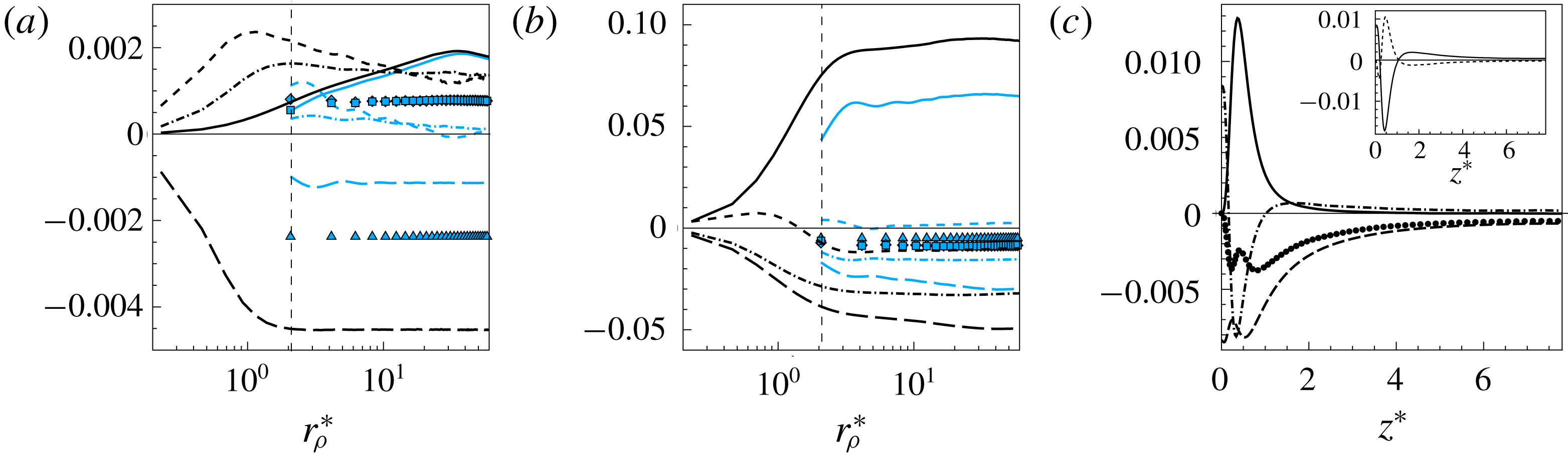
The picture changes when large filter widths are considered, as the resolved physics is strongly affected by the filtering operation and a significant portion of the relevant inhomogeneous mechanisms is left to be taken into account by the SGS heat flux. Accordingly, the scale-by-scale analysis for $\ell _{F}^{\ast }=2.1$ reveals that $\bar{\unicode[STIX]{x1D6F1}}^{\unicode[STIX]{x1D703}}+\bar{T}_{c}^{\unicode[STIX]{x1D703}}<\unicode[STIX]{x1D6F1}^{\unicode[STIX]{x1D703}}+T_{c}^{\unicode[STIX]{x1D703}}$ both in the bulk and in the transitional layer; see figure 11(a,b). In particular, the production is adequately resolved in the bulk, where $\bar{\unicode[STIX]{x1D6F1}}^{\unicode[STIX]{x1D703}}\approx \unicode[STIX]{x1D6F1}^{\unicode[STIX]{x1D703}}$ , but not inside the transitional layer. The reason is given by the fact that in the bulk region the production processes are weak and involve large scales while in the transitional layer production is stronger and small scales are active in the relative mechanisms. Contrary to the production, the transport mechanisms are poorly resolved throughout the entire domain. Hence, the picture consists of resolved fields where the production of temperature variance in the transitional layer is deteriorated and, as a consequence, also the spatial flux that sustains the temperature fluctuations in the other regions of the flow is drastically reduced, i.e. $|\bar{T}_{c}^{\unicode[STIX]{x1D703}}|\ll |T_{c}^{\unicode[STIX]{x1D703}}|$ . For the same reasons, also the resolved cascade mechanisms are strongly depleted, $|\bar{I}_{r}^{\unicode[STIX]{x1D703}}|\ll |I_{r}^{\unicode[STIX]{x1D703}}|$ . As can be expected, this reduction of the forward and reverse transfers in the bulk and transitional layer, respectively, is more pronounced at large resolved scales where the intensity of these two resolved cascade phenomena is found to be almost null.

In agreement with these premises, the role of the SGS heat flux is relevant for the evolution of the resolved fields. In particular, the transport of resolved temperature variance in both physical and scale space is significantly determined by the interaction between resolved and unresolved scales, meaning that the subgrid redistributions $T_{c,sgs}^{\unicode[STIX]{x1D703}}$ and $T_{r,sgs}^{\unicode[STIX]{x1D703}}$ cannot be neglected. The net temperature variance exchange between resolved and subgrid scales is negative both in the bulk and in the transitional layer, $E_{sgs}^{\unicode[STIX]{x1D703}}<0$ . However, this draining is not driven solely by diffusive mechanisms but also by inhomogeneous production and transport mechanisms, which are significant at subgrid level for large filter lengths. As a consequence, the subgrid dissipation does not allow one to recover the unfiltered rate of dissipation, i.e. $|\bar{E}_{e}^{\unicode[STIX]{x1D703}}+E_{sgs}^{\unicode[STIX]{x1D703}}|<|E_{e}^{\unicode[STIX]{x1D703}}|$ .

In order to analyse in more detail the mechanisms determining the behaviour of the subgrid dissipation, $E_{sgs}^{\unicode[STIX]{x1D703}}=-2\langle \unicode[STIX]{x1D712}_{sgs}\rangle$ , we analyse in detail the equation for the subgrid temperature variance $\langle {\unicode[STIX]{x1D703}^{\prime }}^{2}\rangle$ , namely

(4.2) $$\begin{eqnarray}{t_{c}^{\unicode[STIX]{x1D703}}}^{\prime }+{\unicode[STIX]{x1D70B}^{\unicode[STIX]{x1D703}}}^{\prime }-\langle \unicode[STIX]{x1D712}^{\prime }\rangle -t_{c,sgs}^{\unicode[STIX]{x1D703}}+\langle \unicode[STIX]{x1D712}_{sgs}\rangle =0,\end{eqnarray}$$

where the terms denoted with the prime symbol and the ones without it in equation (2.18) are identical except for the replacement of velocity and temperature fields with the subgrid counterparts. Since we consider a spectral cutoff filter, $\langle \bar{\unicode[STIX]{x1D703}}^{2}\rangle +\langle {\unicode[STIX]{x1D703}^{\prime }}^{2}\rangle =\langle \unicode[STIX]{x1D703}^{2}\rangle$ and the sum of the subgrid and the resolved budgets corresponds to the unfiltered one.

Figures 10(c) and 11(c) show the budget (4.2) for $\ell _{F}^{\ast }=0.7$ and $\ell _{F}^{\ast }=2.1$ , respectively. In the case of $\ell _{F}^{\ast }<\ell _{c,min}^{\unicode[STIX]{x1D703}\ast }$ (see figure 10 c), it can be seen that the subgrid dissipation is almost perfectly balanced by the viscous dissipation due to the subgrid scales, $\langle \unicode[STIX]{x1D712}_{sgs}\rangle \approx \langle \unicode[STIX]{x1D712}^{\prime }\rangle$ . The reason is that subgrid production, transport and the subgrid redistribution, ${\unicode[STIX]{x1D70B}^{\unicode[STIX]{x1D703}}}^{\prime }$ , ${t_{c}^{\unicode[STIX]{x1D703}}}^{\prime }$ and $-t_{c,sgs}^{\unicode[STIX]{x1D703}}$ , are negligible inside the bulk of the flow. Closer to the wall, these terms become significant; however, they balance each other and thus they do not contribute to the subgrid dissipation. These results suggest that, for $\ell _{F}^{\ast }<\ell _{c,min}^{\unicode[STIX]{x1D703}\ast }$ , the single relevant phenomenon that the SGS heat flux should take into account is the dissipation occurring at subgrid level. For this reason, as anticipated so far in the analysis of the scale-by-scale budgets, the combination of resolved and subgrid dissipation allows us to recover the unfiltered rate of dissipation, i.e.  $\bar{E}_{e}^{\unicode[STIX]{x1D703}}+E_{sgs}^{\unicode[STIX]{x1D703}}\approx E_{e}^{\unicode[STIX]{x1D703}}$ .

The picture becomes more complicated when large filter widths are considered. As can be seen in figure 11(c), the subgrid dissipation $\langle \unicode[STIX]{x1D712}_{sgs}\rangle$ not only is driven by $\langle \unicode[STIX]{x1D712}^{\prime }\rangle$ but also is influenced by the subgrid production, transport and subgrid redistribution, in order ${\unicode[STIX]{x1D70B}^{\unicode[STIX]{x1D703}}}^{\prime }$ , ${t_{c}^{\unicode[STIX]{x1D703}}}^{\prime }$ and $-t_{c,sgs}^{\unicode[STIX]{x1D703}}$ . In particular, in the bulk of the flow, subgrid production is negligible and subgrid dissipation is driven by the balance between spatial transport and dissipation at subgrid scales, $-\langle \unicode[STIX]{x1D712}_{sgs}\rangle \approx {t_{c}^{\unicode[STIX]{x1D703}}}^{\prime }-t_{c,sgs}^{\unicode[STIX]{x1D703}}-\langle \unicode[STIX]{x1D712}^{\prime }\rangle$ . Close to the wall, also the production at subgrid scales becomes very significant; hence, it does contribute to the value of subgrid dissipation. In conclusion, for large filter lengths, subgrid scales are involved in strong inhomogeneous processes, so that subgrid dissipation does not take into account solely the dissipation at subgrid scales but also production and transport mechanisms. As a result, the sum of resolved and subgrid dissipation does not allow one to recover the unfiltered rate of dissipation, since $|\bar{E}^{\unicode[STIX]{x1D703}}+E_{sgs}^{\unicode[STIX]{x1D703}}|<|E^{\unicode[STIX]{x1D703}}|$ as previously shown in the analysis of the filtered Yaglom equation.

The analysis of the filtered dataset has important implications in LES. Classic eddy-viscosity/diffusivity models may provide a good estimation of the transfers between resolved and subgrid scales when $\ell _{F}^{\ast }<\ell _{c,min}^{\unicode[STIX]{x1D703}}$ , as the main unresolved physics is the dissipation of turbulent kinetic energy and temperature variance. However, the inhomogeneous mechanisms become poorly resolved for larger filters and the SGS fields include highly dynamic eddies that contribute a significant portion of the production and transport besides dissipation, which may lead to modelling issues. Indeed, Smagorinsky-like models cannot account for the inhomogeneous mechanisms occurring at subgrid level; thus the exchanges between resolved and subgrid scales can hardly be copied.

Because the filtered Kolmogorov and the Yaglom equations have been proved to be of great support in describing the turbulent processes at different scales, locations in physical space and filter lengths, then we might consider the filtered scale-by-scale analysis as a valuable tool for testing the SGS models that are commonly employed in LES. This idea has been conceived by Cimarelli & De Angelis (Reference Cimarelli and De Angelis2012) and brought to a novel assessment of the SGS stress model in turbulent channel flow (Cimarelli & De Angelis Reference Cimarelli and De Angelis2014). Future works will continue this line of research and consider the possibility to employ the filtered Kolmogorov and Yaglom equations to evaluate the performances of the state-of-the-art models employed for thermally driven turbulence.