2 A natural deduction system for $\mathsf {LET_C}$

We begin by describing the system $\mathsf {N4^{\star }}$ , an extension of Nelson’s paraconsistent logic $\mathsf {N4}$ with a co-implication operator () and bottom ( $\bot $ ) and top ( $\top $ ) particles. The signature of $\mathsf {N4^{\star }}$ is , and the set of formulas is defined in the usual way. The unary operator $\mathop {\sim }$ is called constructive negation (or strong negation), and a formula can be read as A co-implies B or as B excludes A (cf. [Reference Wansing25, Footnote 2]).

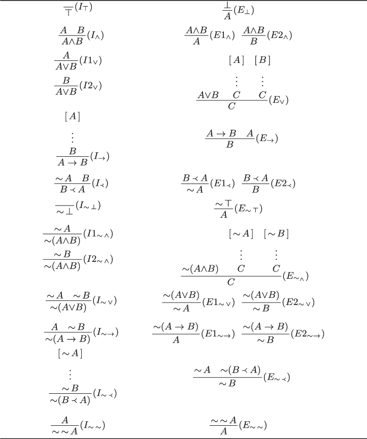
The natural deduction system for $\mathsf {N4^{\star }}$ is presented in Table 1. Analogously as the rules of $\mathsf {Int}$ can be interpreted by means of the existence of proofs, each one of the rules in $\mathsf {N4^{\star }}$ admits an implicit interpretation in terms of evidence: if there is evidence for accepting the formulas in the premises, there is evidence for accepting the formula in the conclusion. Assumptions correspond to the presupposition of existence of evidence (details in Carnielli and Rodrigues [Reference Carnielli and Rodrigues10]).

Table 1

Natural deduction system for $\mathsf {N4^{\star }}$ .

Table 1 Long description

The table is organized into four columns: Connective, Introduction Rule, Elimination Rule, and Rule Name.

* Row 1: Connective is the conjunction symbol. Introduction rule shows A and B above a horizontal line with A wedge B below. Elimination rules show A wedge B above a line with A below, or A wedge B above a line with B below. Rule names are wedge I and wedge E.

* Row 2: Connective is the disjunction symbol. Introduction rules show A above a line with A vee B below, or B above a line with A vee B below. Elimination rule shows A vee B, a derivation of C from assumption A, and a derivation of C from assumption B, all above a line with C below. Rule names are vee I and vee E.

* Row 3: Connective is the implication arrow. Introduction rule shows a derivation of B from assumption A above a line with A arrow B below. Elimination rule shows A and A arrow B above a line with B below. Rule names are arrow I and arrow E.

* Row 4: Connective is the negation symbol. Introduction rule shows a derivation of the bottom symbol from assumption A above a line with neg A below. Elimination rule shows A and neg A above a line with the bottom symbol below. Rule names are neg I and neg E.

* Row 5: Connective is the bottom symbol. There is no introduction rule. Elimination rule shows the bottom symbol above a line with A below. Rule name is bottom E.

* Row 6: Connective is the diamond symbol. Introduction rule shows A above a line with diamond A below. Elimination rule shows diamond A and a derivation of B from assumption A above a line with B below, with a side condition that A is not free in B or other assumptions. Rule names are diamond I and diamond E.

* Row 7: Connective is the box symbol. Introduction rule shows A above a line with box A below. Elimination rule shows box A above a line with A below. Rule names are box I and box E.

The fragment of $\mathsf {N4^{\star }}$ without $\top $ and is equivalent to $\mathsf {N4}^{\bot }$ , which is an Odintsov’s extenstion of $\mathsf {N4}$ with a bottom particle introduced in Odintsov [Reference Odintsov18]. As $\top $ and can be defined in $\mathsf {N4}^{\bot }$ by $\top \stackrel {\scriptscriptstyle\text{def}}{=} \mathop {\sim } \bot $ and , the semantics for $\mathsf {N4}^{\bot }$ presented in Odintsov [Reference Odintsov18] is also adequate for $\mathsf {N4^{\star }}$ .

An equivalence operator $\leftrightarrow $ can be defined in $\mathsf {N4^{\star }}$ as usual $A \leftrightarrow B \stackrel {\scriptscriptstyle\text{def}}{=} (A \to B) {\wedge } (B \to A)$ . As in $\mathsf {N4}$ , substitution by equivalent formulas in $\mathsf {N4^{\star }}$ is not valid. For instance, in $\mathsf {N4^{\star }}$ the equivalence is provable, whereas the equivalence is not provable. However, a strong equivalence operator $\Leftrightarrow $ can be defined by $A \Leftrightarrow B \stackrel {\scriptscriptstyle\text{def}}{=} (A \leftrightarrow B) {\wedge } (\mathop {\sim } A \leftrightarrow \mathop {\sim } B)$ , and substitution by strongly equivalent formulas is valid.

In $\mathsf {N4^{\star }}$ , the connectives ${\wedge }$ and ${\vee }$ are dual, because $A {\vee } B$ is strongly equivalent to $\mathop {\sim } (\mathop {\sim } A {\vee } \mathop {\sim } B)$ (these formulas are practically the same in this system). Moreover, the connectives $\to $ and can also be seen as dual, because is strongly equivalent to $\mathop {\sim } (\mathop {\sim } A \to \mathop {\sim } B)$ (which can be easily proven using the rules in Table 1). It is therefore possible to define the connectives ${\vee }$ and in terms of the connectives ${\wedge }$ , $\to $ and $\mathop {\sim }$ , rather than regarding them as primitive. Nevertheless, we consider ${\vee }$ and to be primitive connectives. This is with the aim of making the duality between the connectives and the symmetry between truth and falsity more evident.

In $\mathsf {N4^{\star }}$ , an intuitionistic negation $\mathop {\neg }$ is defined by $\mathop {\neg } A \stackrel {\scriptscriptstyle\text{def}}{=} A \to \bot $ and a co-negation is defined by . While the intention of Nelson’s constructive negation is to express falsity (i.e., $\mathop {\sim } A$ must be interpreted as ‘A is false’, cf. Nelson [Reference Nelson17]), intuitionistic negation must be interpreted as expressing impossibility of truth (i.e., $\mathop {\neg } A$ must be interpreted as ‘it is impossible that A be true’ or as ‘it is impossible to construct a proof of A’, cf. Shramko [Reference Shramko23]). Accordingly, the formula , which is strongly equivalent to $\mathop {\neg } \mathop {\sim } A$ , must be understood as the impossibility of the falsity of A. Under such interpretations, the following theorem shows that, in $\mathsf {N4^{\star }}$ , the falsity of a formula A is not equivalent to the impossibility of the truth of A (item 1), and the truth of a formula A is not equivalent to the impossibility of the falsity of A (item 2). However, the falsity of a formula A is equivalent to the falsity of the impossibility of the falsity of A (item 3), and the truth of a formula A is equivalent to the falsity of the impossibility of the truth of A (item 4). The other items show additional properties of the interaction between negations in $\mathsf {N4^{\star }}$ .

It is important to highlight that the distinctions between truth and impossibility of falsity, and between falsity and impossibility of truth, cannot be made in other logics, such as classical or intuitionistic logic. These are remarkable features of $\mathsf {N4^{\star }}$ that are important for the constructive properties of this logic, as explained in Section 6.

The following theorem shows some properties of formulas related with the principles of explosiveness (or ex contradictione [sequitur] quodlibet) and excluded middle (or tertium non datur) in $\mathsf {N4^{\star }}$ .

The previous theorem motivates the following definitions of connectives for consistency ( $\mathop {\circ }$ ), inconsistency ( $\mathop {\bullet }$ ), determinedness (), and undeterminedness (). The logic $\mathsf {LET_C}$ is the result of adding to $\mathsf {N4^{\star }}$ such definitions.

Note that although the definition of the consistency connective is similar to the one proposed by da Costa in his well-known hierarchy of Inconsistent Formal Systems $\mathsf {C_n}$ , our definition differs in a significant way. We employ two negations in place of one, with each negation representing a distinct concept (namely the impossibility of truth and falsity).

The following properties are immediate from the previous definition of connectives and theorems.

3 Adding lambda-terms to $\mathsf {LET_C}$ : making evidence explicit

A BHK-style interpretation of $\mathsf {LET_C}$ in terms of evidence for accepting or rejecting propositions is presented below. This informal interpretation gives us the intuitions for adding lambda terms to $\mathsf {LET_C}$ . The emptyset symbol ( $\emptyset $ ) is used to represent evidence for accepting propositions which are self-evident (i.e., propositions accepted without need of proofs or explanations):

• • Evidence for accepting $A {\wedge } B$ is a pair $(e_1, e_2)$ where $e_1$ is evidence for accepting A and $e_2$ is evidence for accepting B.

• • Evidence for accepting $A {\vee } B$ is a pair $(e_1, e_2)$ where $e_1 = 0$ and $e_2$ is evidence for accepting A, or $e_1 = 1$ and $e_2$ is evidence for accepting B.

• • Evidence for accepting $A \to B$ is a method that converts evidence for accepting A into evidence for accepting B.

• • Evidence for accepting is a pair $(e_1, e_2)$ where $e_1$ is evidence for rejecting A and $e_2$ is evidence for accepting B.

• • Evidence for accepting $\mathop {\sim } A$ is evidence for rejecting A.

• • There is no evidence for accepting $\bot $ .

• • $\emptyset $ is evidence for accepting $\top $ .

• • Evidence for rejecting $A {\wedge } B$ is a pair $(e_1, e_2)$ where $e_1 = 0$ and $e_2$ is evidence for rejecting A, or $e_1 = 1$ and $e_2$ is evidence for rejecting B.

• • Evidence for rejecting $A {\vee } B$ is a pair $(e_1, e_2)$ where $e_1$ is evidence for rejecting A and $e_2$ is evidence for rejecting B.

• • Evidence for rejecting $A \to B$ is a pair $(e_1, e_2)$ where $e_1$ is evidence for accepting A and $e_2$ is evidence for rejecting B.

• • Evidence for rejecting is a method that converts evidence for rejecting A into evidence for rejecting B.

• • Evidence for rejecting $\mathop {\sim } A$ is evidence for accepting A.

• • $\emptyset $ is evidence for rejecting $\bot $ .

• • There is no evidence for rejecting $\top $ .

Note that the previous clauses only state what constitutes evidence for accepting or rejecting compound formulas, based on evidence for accepting or rejecting their constituent parts. There is no clauses stating what constitute evidence for accepting or rejecting propositional variables because, as argued in Carnielli and Rodrigues [Reference Carnielli and Rodrigues10], it depends on the area of study and the subject matter, and this is not a problem of logic.

In order to explicitly express evidence, based on the previous informal interpretation of $\mathsf {LET_C}$ , lambda-terms from an extended lambda calculus ( $\lambda _C$ -calculus) are added to $\mathsf {LET_C}$ , obtaining $\mathsf {LET_C^{\lambda }}$ . The $\lambda _C$ -calculus is an extension of the pure lambda-calculus with (two kinds of) pairs and projections, injections, case distinction, empty term, impossible (or exception) terms, and (two kinds of) identities.Footnote ¹ $\mathsf {LET_C^{\lambda }}$ is really a type system whose types are the formulas of $\mathsf {LET_C}$ and whose terms are the elements of the $\lambda _C$ -calculus. Two kinds of pairs and projections are used to ensure the uniqueness of types (module strong equivalence). The first kind will be used for conjunctions and negations of disjunctions, while the second kind will be used for co-implications and negation of implications. Pairs of the second kind will be called combined pairs, since they always have a term of a formula and a term of a negated formula. The two kinds of identities are used to differentiate terms of formulas and of their double strong negations.

To define the set of terms of the $\lambda _C$ -calculus, we consider a denumerable set of variables V, whose elements represent the evidence that is assumed to exist. We shall use the last letters (possibly with subscripts) of the Latin alphabet $x, x_1, \ldots , y, y_1, \ldots $ to denote elements of V, and letters $r, s, t$ to denote arbitrary $\lambda _C$ -terms.

Definition 3.1. The set of terms of the $\lambda _C$ -calculus, denoted by $\Lambda $ , is defined by the following grammar:

$$ \begin{align*} \Lambda = &V \;|\; & \text{ (variables)} \\ &\lambda V.\Lambda \;|\; \text{ap}(\Lambda, \Lambda) \;|\; & \text{ (abstractions and applications)} \\ &(\Lambda, \Lambda) \;|\; \pi_1(\Lambda) \;|\; \pi_2(\Lambda) \;|\; & \text{ (pairs and projections)} \\ &\langle \Lambda, \Lambda\rangle \;|\; \pi_1^*(\Lambda) \;|\; \pi_2^*(\Lambda) \;|\; & \text{ (combined pairs and projections)} \\ &\text{in}_1(\Lambda) \;|\; \text{in}_2(\Lambda) \;|\; & \text{ (injections)} \\ &\text{case } \Lambda \text{ of } [V] \Lambda \text{ or } [V] \Lambda \;|\; & \text{ (case distintion)} \\ &\emptyset \;|\; \mathcal{E}(\Lambda) \;|\; & \text{ (empty and exception terms)}\\ &\text{id}(\Lambda) \;|\; \text{id}^{-1}(\Lambda) & \text{ (identities).} \end{align*} $$

We shall use $r[x := s]$ to denote the result of substituting s for the free occurrences of x in r (changing bound variables to fresh variables if necessary to avoid creating new occurrences of bound variables). The $\beta $ -reduction relation on $\Lambda $ is defined as follows.

Definition 3.2. The one step $\beta $ -reduction relation on $\Lambda $ , denoted by $\rightarrow _{\beta }$ , is the least compatible relation on $\Lambda $ with base rules:Footnote ²

$$ \begin{align*} \text{ap}(\lambda x.r, s) &\rightarrow_{\beta} r[x := s] \\ \pi_1((r, s)) &\rightarrow_{\beta} r \\ \pi_2((r, s)) &\rightarrow_{\beta} s \\ \pi_1^*(\langle r, s\rangle) &\rightarrow_{\beta} r \\ \pi_2^*(\langle r, s\rangle) &\rightarrow_{\beta} s \\ \text{case } \text{in}_1(t) \text{ of } [x] r \text{ or } [y] s &\rightarrow_{\beta} r[x:=t] \\ \text{case } \text{in}_2(t) \text{ of } [x] r \text{ or } [y] s &\rightarrow_{\beta} s[y:=t] \\ \text{id}(\text{id}^{-1}(t)) &\rightarrow_{\beta} t \\ \text{id}^{-1}(\text{id}(t)) &\rightarrow_{\beta} t. \end{align*} $$

The multi-step $\beta $ -reduction relation on $\Lambda $ , denoted by $\twoheadrightarrow _{\beta }$ , is the reflexive and transitive closure of $\rightarrow _{\beta }$ .

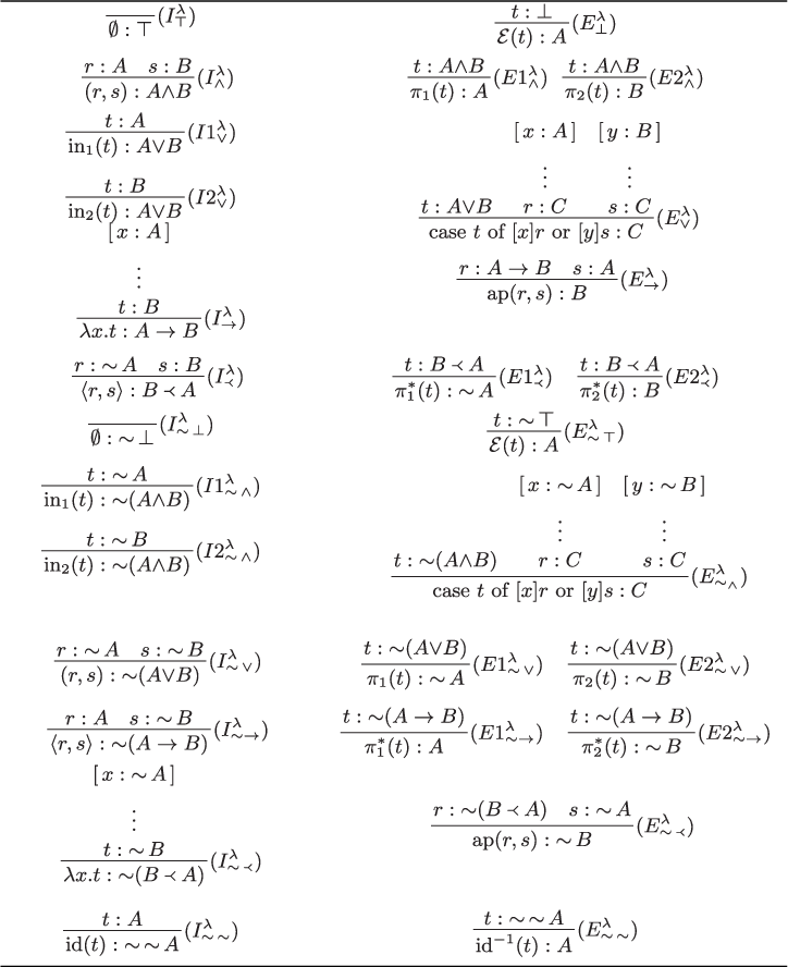
We shall use $\mathcal {F}(\mathsf {LET_C})$ to denote the set of formulas of $\mathsf {LET_C}$ . The notions of statement, declaration, context and judgement are defined as usual in type systems: A statement is an expression of the form $t:A$ , where $t \in \Lambda $ and $A \in \mathcal {F}(\mathsf {LET_C})$ (in such a statement t is called the subject); a declaration is a statement with a variable as subject; a context is a set of declarations with different subjects; and a judgement has the form $\Gamma \vdash t:A$ , with $\Gamma $ a context and $t:A$ a statement. A judgement $\Gamma \vdash t:A$ in $\mathsf {LET_C^{\lambda }}$ means that there is a derivation of statement $t:A$ , with open declarations (or assumptions) in $\Gamma $ , using the rules in Table 2. Intuitively, $x_1 : B_1, \ldots , x_n : B_n \vdash t : A$ means that if we consider that $x_i$ represents evidence for accepting $B_i$ , for $1 \leq i \leq n$ , then t represents evidence for accepting A (evidence for accepting $\mathop {\sim } B$ is the same that evidence for rejecting B).

Table 2

Natural deduction system for $\mathsf {LET_C^{\lambda }}$

Table 2 Long description

The table is divided into four sections.

1. Axioms: Located at the top, showing the rule Ax where Gamma unioned with the set containing A entails A.

2. Implication Rules:

- Introduction rule: If Gamma unioned with A entails B, then Gamma entails A implies B.

- Elimination rule: If Gamma entails A implies B and Gamma entails A, then Gamma entails B.

3. Conjunction Rules:

- Introduction rule: If Gamma entails A and Gamma entails B, then Gamma entails A and B.

- Elimination rules: Two rules showing that if Gamma entails A and B, then Gamma entails A; and if Gamma entails A and B, then Gamma entails B.

4. Disjunction Rules:

- Introduction rules: Two rules showing that if Gamma entails A, then Gamma entails A or B; and if Gamma entails B, then Gamma entails A or B.

- Elimination rule: If Gamma entails A or B, and Gamma unioned with A entails C, and Gamma unioned with B entails C, then Gamma entails C.

The following theorem, which has a simple proof, shows that $\mathsf {LET_C^{\lambda }}$ actually achieves the objective for which it was designed: to formalise evidence in an explicit way. Moreover, the lambda terms and their reduction rules give us procedures to calculate evidence of compound formulas from their constituent parts.

4 Some properties of $\mathsf {LET_C^{\lambda }}$

In this section, some usual properties of type systems are proven for $\mathsf {LET_C^{\lambda }}$ . Before that, some definitions are necessary.

The set of free variables of terms $t \in \Lambda $ , denoted by $\text {FV}(t)$ , is defined as usual (the only binding operators are $\lambda $ in abstractions and $[\cdot ]$ in case distinctions).

Theorem 4.8 (Normalisation Theorem).

Every legal term is strongly normalising.

Proof Let us consider the simple typed $\lambda $ -calculus extended with products, sums, empty type and unity type (denoted by ${\wedge }$ , ${\vee }$ , $\bot $ , and $\top $ , respectively). This calculus, which we will denoted by $\mathsf {E}^{\lambda }$ , is a fragment of $\mathsf {LET_C^{\lambda }}$ ( $\mathsf {E}^{\lambda }$ is $\mathsf {LET_C^{\lambda }}$ dropping the rules for co-implication and constructive negation), and can also be seen as a fragment of Intuitionistic Type Theory ( $\mathsf {ITT}$ ) (in the version presented in Martin-Löf [Reference Martin-Löf15], for instance). Therefore, the strong normalisation of $\mathsf {ITT}$ implies the strong normalisation of $\mathsf {E}^{\lambda }$ . A term translation function $\varphi $ , from terms of the $\lambda _C$ -calculus to terms of the extended $\lambda $ -calculus used in $\mathsf {E}^{\lambda }$ , can be defined by:

Considering that the types of $\mathsf {E}^{\lambda }$ are generated by the set of propositional variables $V' = V \cup \{\overline {p} \;|\; p \in V \}$ , a type translation function $\psi $ , from types of $\mathsf {LET_C^{\lambda }}$ to types of $\mathsf {E}^{\lambda }$ , can be defined by:

By induction on t, it can be proven that if $\Gamma \vdash t:A$ in $\mathsf {LET_C}$ , then $\{\varphi (s):\psi (B) \;|\; s:B \in \Gamma \} \vdash \varphi (t):\psi (A)$ in $\mathsf {E}^{\lambda }$ . Moreover, if t has an infinite reduction chain in $\lambda _C$ -calculus, then $\varphi (t)$ has an infinite reduction chain in the extended $\lambda $ -calculus used in $\mathsf {E}^{\lambda }$ . Consequently, as $\mathsf {E}^{\lambda }$ satisfies strong normalisation, then $\mathsf {LET_C^{\lambda }}$ satisfies strong normalisation.

5 Realisability interpretation for $\mathsf {LET_C}$

A realisability interpretation of Heyting Arithmetic ( $\mathsf {HA}$ ) was proposed in Kleene [Reference Kleene14]. Under such interpretation, codes of recursive functions are assigned to provable formulas of $\mathsf {HA}$ , establishing in this way a connection between provability in $\mathsf {HA}$ and recursive functions, which in a certain way justifies that $\mathsf {Int}$ is indeed constructive (at least in the formalisation of arithmetic). Nelson [Reference Nelson17] extends Kleene’s notion of realisability interpreting arithmetic formulas by two recursively and simultaneously defined notions of positive realisability (P-realisability) and negative realisability (N-realisability), and presents a formal system of number theory, to which we shall refer as Nelson Arithmetic ( $\mathsf {NA}$ ), that satisfies such realisability interpretations. $\mathsf {NA}$ is basically the result of substituting the axioms for (intuitionistic) negation in $\mathsf {HA}$ by axioms of a constructive negation, which formalises constructive falsity in a dual way of constructive truth. The logic axioms of $\mathsf {NA}$ are what comprise what is currently known as Nelson’s Logic, and a variation of this logic (presented in Almukdad and Nelson [Reference Almukdad and Nelson1]), in which the explosiveness of the constructive negation is avoided, is currently known as Nelson’s Paraconsistent Logic. As previously mentioned, the propositional fragment of Nelson’s paraconsistent logic is usually denoted by $\mathsf {N4}$ . Based on Nelson’s notions of positive and negative realisabilty, dropping the clauses for elementary arithmetical formulas and for quantifiers, and adding some clauses for , $\bot $ and $\top $ , the realisability interpretation of formulas of $\mathsf {N4^{\star }}$ (and also of $\mathsf {LET_C}$ ) can be defined as follows, where $\text {p}(\cdot , \cdot )$ denote a fixed primitive recursive bijection from $\mathbb {N}^2$ to $\mathbb {N}$ (a pair coding function), and $\varphi _l$ is the partial recursive function with index l (under some fixed enumeration of the partial recursive functions).

In order to make more intuitive the relationship between P-realisability and provability in $\mathsf {LET_C}$ (Theorem 5.2 below), and also to establish a connection with our explicit representation of evidence by means of $\lambda _C$ -terms, we shall consider that evidence is codified by natural numbers, thus every assignation of natural numbers to free variables of $\lambda _C$ -terms, in a deduction in $\mathsf {LET_C^{\lambda }}$ , will give as a particular justification of such deduction based on evidence.

Note that there are no clauses for the P-realisation or the N-realisation of propositional variables, consequently formulas $p {\vee } \mathop {\sim } p$ and $\mathop {\sim } (p {\wedge } \mathop {\sim } p)$ , with $p \in V$ , have no P-realisers. This justifies the paracomplete and paraconsistent character of $\mathsf {LET_C}$ .

In Rose [Reference Rose22], it is proved that there exists an intuitionistic propositional formula for which the substitution of number-theoretic formulas for its propositional variables produces realisable but not intuitionistically provable formulas. Although our definition of P-realisability and N-realisability of formulas of $\mathsf {N4^{\star }}$ does not depend on an arithmetic (or any other) theory, Rose’s result and the fact that $\mathsf {N4^{\star }}$ is a conservative extension of intuitionistic propositional logic (cf. [Reference Odintsov18, Corollary 8.6.6]) are strong reasons to believe that the reciprocal of Corollary 5.3 and of Theorem 5.2 are not valid.

6 On the constructivity of $\mathsf {LET_C}$

As stated in [Reference Wansing25, pp. 341–342]:

Some reasons to justify that $\mathsf {LET_C}$ is a constructive logic are the following:

• • $\mathsf {LET_C}$ does not satisfy the Principle of Excluded Middle (PEM). According to [Reference Negri and von Plato16, p. 27], “Under the constructive interpretation, the law of excluded middle is not an empty “tautology,” but expresses the decidability of proposition A.” The failure of PEM is then related to the existence of undecidable propositions, and is usually used to justify that a logic is constructive. The decidability of a particular proposition A can be expressed in $\mathsf {LET_C}$ by .

• • $\mathsf {LET_C}$ satisfies the disjunction property (i.e., if $\vdash A {\vee } B$ , then $\vdash A$ or $\vdash B$ ).Footnote ³ This is another property usually used to justify that a logic is constructive.

• • $\mathsf {LET_C}$ also satisfies the (negation of) conjunction property (i.e., if $\vdash \mathop {\sim } (A {\wedge } B)$ , then $\vdash \mathop {\sim } A$ or $\vdash \mathop {\sim } B$ ),Footnote ⁴ which can be viewed as a constructive property dual to the disjunction property.

• • As it was shown in Section 3, $\mathsf {LET_C}$ admits a BHK-style interpretation where evidence for accepting or rejecting compound propositions are treated as constructions, in an analogous way as the BHK-interpretation for $\mathsf {Int}$ offers a constructive interpretation of that logic in terms of proofs.

• • The system $\mathsf {LET_C^{\lambda }}$ provides an explicit representation of evidence by means of $\lambda _C$ -calculus terms, which represent algorithmic procedures to calculate evidence of compound propositions base on evidence for their constituent parts.

• • The realisability interpretation provided for $\mathsf {LET_C}$ , Theorem 5.2 and Corollary 5.3 establish a strong connection between derivations in $\mathsf {LET_C}$ and recursive functions, which also highlights the algorithmic nature of the evidence building process in $\mathsf {LET_C}$ .

Since the classical negation of a proposition is true iff the proposition is false, classical negation expresses falsity. Moreover, the classical negation of a proposition A can be defined as the intuitionistic negation (i.e., as $A \to \bot $ ), which can be interpreted as the impossibility of A be true. Consequently, in classical logic there is no distinction between falsity and impossibility of truth. Intuitionistically, it is less clear whether or not there is a distinction between falsity and impossibility of truth. Although Shramko [Reference Shramko23] recognises that “There is a tradition to present intuitionistic falsity of a sentence as truth of its (intuitionistic) negation.” and claims that “Brouwer and Heyting seem not to have any special conception of falsity as a philosophical (or semantic) notion. Whenever they occasionally speak of falsity, they simply mean intuitionistic negation.”, he proposes a “genuine intuitionistic notion of falsity” which is not captured by the intuitionistic negation. On the other hand, as shown in Section 2, in $\mathsf {LET_C}$ the notions of falsity and impossibility of truth are clearly separated.

From a constructive point of view, it seems clear that $\mathsf {Int}$ allows only direct proofs to establish the truth of propositions. However, if it is accepted that intuitionistic negation represents intuitionistic falsity, then $\mathsf {Int}$ allows only indirect proofs to establish the falsity of propositions. Consequently, if by a “constructive proof” we mean a “direct proof”, under the interpretation of negation as falsity, $\mathsf {Int}$ allows only constructive proofs to establish the truth of propositions and no constructive proofs to establish the falsity of propositions. However, if we understand intuitionistic negation as impossibility of truth, $\mathsf {Int}$ not only allows constructive (or direct) proofs to establish the truth of propositions, but also to establish the impossibility of the truth of propositions. In our view, the correct interpretation of intuitionistic negation is the later one, and we agree with Shramko that intuitionistic negation does not represent falsity. The failure of the (negation of) conjunction property in $\mathsf {Int}$ can be seen as a consequence of the fact that the intuitionistic negation does not represent falsity.

In $\mathsf {LET_C}$ , the constructive negation represents falsity (i.e., $\mathop {\sim } A$ can be interpreted as “A is false”), the intuitionistic negation represents impossibility of truth (i.e., $\mathop {\neg } A$ must be interpreted as “it is impossible that A be true”), and the constructive negation of co-intuitionistic negation represents impossibility of falsity (i.e., must be interpreted as “it is impossible that A be false”). As it was shown in Section 2, these notions are separated in $\mathsf {LET_C}$ . From a constructive point of view, $\mathsf {LET_C}$ allows only direct proofs to establish the truth of propositions and the impossibility of the truth of propositions, and also allows only direct proofs to establish the falsity of propositions and the impossibility of the falsity of propositions. Taking “direct proof” as a synonym for “constructive proof”, it follows that $\mathsf {LET_C}$ is constructively richer than $\mathsf {Int}$ .

Intuitively, it seems reasonable to infer the falsity of a proposition from the impossibility of its truth, and the truth of a proposition from the impossibility of its falsity, which leads us to consider the inclusion of the following rules to $\mathsf {LET_C}$ (taking into account that and $\mathop {\neg } \mathop {\sim } A$ are strongly equivalent in $\mathsf {LET_C}$ ):

However, it is easy to show that the inclusion of these rules makes admissible the following rules:

which can be seen as indirect proofs (or proofs by reductio ad absurdum) for the truth or the falsity of A, respectively. Using the rule $(E_{\mathop {\sim } \mathop {\sim }})$ , it can be proven that $(E_{\mathop {\neg }})$ makes admissible $(E_{\mathop {\neg } \mathop {\sim }})$ , and that $(E_{\mathop {\neg } \mathop {\sim }})$ makes admissible $(E_{\mathop {\neg }})$ . Consequently, the addition of either of these two rules to $\mathsf {LET_C}$ will cause the system to lose its constructivist properties.

It can also be considered reasonable that the falsity of a proposition implies the impossibility of its truth, and that the truth of a proposition implies the impossibility of its falsity, which would lead us to consider adding the following rules to $\mathsf {LET_C}$ :

It can also be proven that the addition of $(I_{\mathop {\neg }})$ makes admissible $(I_{\mathop {\neg } \mathop {\sim }})$ , and that the addition of $(I_{\mathop {\neg } \mathop {\sim }})$ makes admissible $(I_{\mathop {\neg }})$ . Moreover, it is evident that the addition of ( $I_{\mathop {\neg }}$ ) to $\mathsf {LET_C}$ will make the constructive negation explosive. Consequently, the addition of $(I_{\mathop {\neg } })$ or $(I_{\mathop {\neg } \mathop {\sim }})$ to $\mathsf {LET_C}$ will result in the system becoming non-paraconsistent, and no longer able to formalise deductions in contexts with conflicting information.

7 Concluding remarks and future work

This article introduces the constructive logic of evidence and truth, $\mathsf {LET_C}$ , a new system within the family of LETs. The logic $\mathsf {LET_C}$ extends $\mathsf {N4^{\star }}$ (an extension of Nelson’s paraconsistent logic) by adding connectives for consistency, inconsistency, determinedness, and undeterminedness. Unlike other LETs, which feature a classicality operator that simultaneously restores the consistency and determinacy of certain propositions, $\mathsf {LET_C}$ provides distinct connectives for the independent recovery of these properties.

Lambda-calculus terms were incorporated into $\mathsf {LET_C}$ , resulting in the type system $\mathsf {LET_C^{\lambda }}$ , which provides an explicit formalisation of evidence. This approach contrasts with the one presented in Fitting [Reference Fitting12]. In $\mathsf {LET_C^{\lambda }}$ , lambda-calculus terms not only represent evidence but also describe algorithmic procedures for deriving evidence for compound formulas based on evidence for their constituent parts.

The Justification Logics proposed in Artemov [Reference Artemov5] generalize the Logic of Proofs ( $\mathsf {LP_{0}}$ ), introduced by the same author in Artemov [Reference Artemov3] and further developed in Artemov [Reference Artemov4] and Artemov and Fitting [Reference Artemov and Fitting6]. $\mathsf {LP_{0}}$ formalises the Brouwer–Heyting–Kolmogorov (BHK) provability interpretation of Intuitionistic Logic, with proofs explicitly represented as ‘proof polynomials.’ This formalisation leads to an embedding within Peano Arithmetic. However, as noted in the introduction, the goals and methods of $\mathsf {LET_C}$ differ significantly from those of justification logics, particularly from $\mathsf {LP_{0}}$ . Nevertheless, it remains an open possibility to apply $\mathsf {LP_{0}}$ -like techniques to formalise the BHK-style interpretation of $\mathsf {LET_C}$ , where ‘evidence’ is understood as ‘proof’ within Nelson’s arithmetic system.

In addition to the algorithmic interpretation offered by the lambda-calculus terms in $\mathsf {LET_C^{\lambda }}$ , a realisability interpretation is also offered for $\mathsf {LET_C}$ which highlights the constructive properties of this logic, establishing a close relationship between deductions and recursive functions.

As previously stated in Section 6, $\mathsf {LET_C}$ is a logic that extends $\mathsf {Int}$ , generating new constructivist properties. $\mathsf {LET_C}$ enables not only constructive demonstrations for the truth and the impossibility of truth of propositions, but also for the falsity and the impossibility of falsity of propositions. The separation between truth and impossibility of falsity, and between falsity and impossibility of truth, is a key component for $\mathsf {LET_C}$ to achieve its constructivist properties.

Extending $\mathsf {LET_C}$ to a first-order logic is not particularly difficult. This can be achieved by incorporating the rules for the quantifiers $\forall $ and $\exists $ , along with their negations, as done in Nelson’s logic with quantifiers. Additionally, the rules for dependent types ( $\Pi $ -types and $\Sigma $ -types) allow to extend $\mathsf {LET_C^{\lambda }}$ to a system that includes types for the quantifiers and their negations. The realisability interpretation also appears to extend naturally to a first-order version of $\mathsf {LET_C}$ . However, these extensions are not presented in this article, as we believe that the most interesting aspects of our proposal are already captured at the propositional level.

As mentioned in the Introduction, $\mathsf {LET_C}$ formalises an instantaneous view of evidence-based deductions, where reasoning is based solely on the current available information. To capture a more dynamic perspective—where an agent can revise or incorporate new evidence based on their deductions—it may be valuable to develop a meta-reasoning architecture (meta-logic) for $\mathsf {LET_C}$ . This meta-reasoning could allow for the modification of hypotheses (or theories) according to reasonable criteria. Such an approach would separate reasoning based on existing evidence (formalised within the logical system) from reasoning about the evidence itself (which would be formalised in the meta-logic). This presents an exciting avenue for future research.

Although much theoretical and technical work remains before $\mathsf {LET_C}$ can be applied to the automation of reasoning in contexts involving conflicting and insufficient information, it is worth noting that the concept of constructive justification may be particularly well-suited for exploring algorithmic explainability in the context of Artificial Intelligence.