



1. Introduction
Thermal convection is a ubiquitous phenomenon in natural environments, playing an important role in many geophysical and astrophysical systems (Hartmann et al. Reference Hartmann, Moy and Fu2001; Hanasoge et al. Reference Hanasoge, Gizon and Sreenivasan2016; Wicht & Sanchez Reference Wicht and Sanchez2019; Hartmann et al. Reference Hartmann, Stevens, Lohse and Verzicco2024). Fluids subjected to uneven heating under gravitational fields generate motion due to buoyancy, with heat being converted into kinetic energy driving large-scale turbulent motion. As one typical paradigm of thermal convection, Rayleigh–Bénard convection (RBC), wherein the flow is heated below and cooled above, has attracted considerable attention over the past few decades (Grossmann & Lohse Reference Grossmann and Lohse2000; Ahlers et al. Reference Ahlers, Grossmann and Lohse2009; Lohse & Xia Reference Lohse and Xia2010; Chillà & Schumacher Reference Chillà and Schumacher2012; Yeh Reference Yeh2023; Lohse & Shishkina Reference Lohse and Shishkina2024). In the traditional planar RBC system, regular large-scale circulation (LSC) formed by upward-moving hot plumes and downward-moving cold plumes, is the primary flow structure, continuously transferring heat from the lower plate to the upper plate (Grossmann & Lohse Reference Grossmann and Lohse2000, Reference Grossmann and Lohse2001; Xia Reference Xia2013). In other variants of RBC, such as centrifugal convection (CC) in an annular structure (Jiang et al. Reference Jiang, Zhu, Wang, Huisman and Sun2020; Rouhi et al. Reference Rouhi, Lohse, Marusic, Sun and Chung2021; Jiang et al. Reference Jiang, Wang, Liu and Sun2022; Bhadra et al. Reference Bhadra, Shishkina and Zhu2024, Reference Bhadra, Shishkina and Zhu2025; Lai et al. Reference Lai, Zhong and Sun2025; Wang et al. Reference Wang, Liu, Lai and Sun2024; Yao et al. Reference Yao, Emran, Teimurazov and Shishkina2025) and turbulent spherical RBC in a spherical shell (Fan et al. Reference Fan, Wang and Lin2024; Fu et al. Reference Fu, Bader, Song and Zhu2024), the roll-like large-scale organisation remains well preserved and continues to serve as the primary structure for heat transfer within the classical regime.
In real-world natural and industrial settings, thermal convection typically develops under complex conditions, in which multiple factors can disrupt the LSC and thereby alter heat transfer efficiency. Externally imposed flows – such as Couette flows driven by boundary motion or pressure-driven Poiseuille flows – can effectively disrupt LSC patterns (Blass et al. Reference Blass, Zhu, Verzicco, Lohse and Stevens2020; Leng et al. Reference Leng, Krasnov, Li and Zhong2021; Zhong et al. Reference Zhong, Wang and Sun2023b ; Yerragolam et al. Reference Yerragolam, Howland, Stevens, Verzicco, Shishkina and Lohse2024; Zhong et al. Reference Zhong, Li, Zhou and Sun2025). Under such background shear, vertical plumes become deflected, large-scale convection rolls are stretched and eventually break up, plume generation is hindered and the overall heat transfer efficiency is notably reduced (Yerragolam et al. Reference Yerragolam, Verzicco, Lohse and Stevens2022; Zhong et al. Reference Zhong, Li and Sun2024). Rotational effects can also modify the flow structure through the action of the Coriolis force. According to the Taylor–Proudman constraint, when rotation is sufficiently strong, the primary flow in a rotating RBC develops into vertically aligned Taylor columns that connect the top and bottom plates (King et al. Reference King, Stellmach, Noir, Hansen and Aurnou2009; Kunnen et al. Reference Kunnen, Stevens, Overkamp, Sun, Van Heijst and Clercx2011, Reference Kunnen, Clercx and Van Heijst2013; King & Aurnou Reference King and Aurnou2013; Ecke & Shishkina Reference Ecke and Shishkina2023; Song et al. Reference Song, Shishkina and Zhu2024a , Reference Song, Shishkina and Zhub ). The presence of a porous medium may suppress thermal convection as well. When the medium is relatively sparse, large-scale flow structures remain largely intact; however, as its density increases and permeability decreases, the accompanying rise in viscous resistance destabilises these structures, leading heat transfer to occur predominantly through individual plume flows (Liu et al. Reference Liu, Jiang, Chong, Zhu, Wan, Verzicco, Stevens, Lohse and Sun2020; Xu et al. Reference Xu, Xu and Xi2023; Zhong et al. Reference Zhong, Liu and Sun2023a ; Zhu et al. Reference Zhu, Fu and De Paoli2024; Li et al. Reference Li, Yang and Sun2025).
In addition, another crucial factor that governs flow patterns and heat transfer is the boundary condition of the system. In the canonical RBC set-up, no-slip and isothermal boundary conditions are imposed on both the top and bottom plates, while periodic conditions are applied along the horizontal directions. Temporal or spatial modulations of the boundary temperature can influence plume fluctuations and spacing, and even significantly enhance heat transfer efficiency through carefully designed temperature distributions (Yang et al. Reference Yang, Chong, Wang, Verzicco, Shishkina and Lohse2020; Zhao et al. Reference Zhao, Zhang, Wang, Wu, Chong and Zhou2022; Zhou & Zhu Reference Zhou and Zhu2025). Regarding velocity boundary conditions, stress-free boundaries provide a favourable environment for the emergence of zonal flows owing to their reduced viscous dissipation. Two distinct flow states – zonal flow and convection rolls – have been identified in two-dimensional RBC with stress-free plates and periodic lateral boundaries. These two states were initially found to coexist under identical parameter conditions and were shown to be strongly influenced by the initial state and the system’s aspect ratio (Goluskin et al. Reference Goluskin, Johnston, Flierl and Spiegel2014; van der Poel et al. Reference van der Poel, Ostilla-Mónico, Verzicco and Lohse2014; Wang et al. Reference Wang, Chong, Stevens, Verzicco and Lohse2020; Wen et al. Reference Wen, Goluskin, LeDuc, Chini and Doering2020). Through extensive direct numerical simulations with prolonged integration times, Wang et al. (Reference Wang, Goluskin and Lohse2023) further demonstrated that zonal flow is metastable at moderate Rayleigh numbers, eventually decaying into the roll state after a finite lifetime with survival probability decreasing exponentially in time.
However, in geophysical and astrophysical systems, zonal flows are commonly observed to persist over long times, for example in the global atmospheric circulation and in Jupiter’s zonal winds (Schneider Reference Schneider2006; Yadav et al. Reference Yadav, Heimpel and Bloxham2020; Heimpel et al. Reference Heimpel, Yadav, Featherstone and Aurnou2022). This contrast raises the question of what additional mechanisms may control the formation and long-term stability of zonal flow. In particular, it remains unclear how rotation and geometric curvature, and their interplay, shape the emergence of zonal flow and the associated heat transfer. Moreover, real-world flows often involve mixed velocity boundary conditions, with one boundary no slip and the other stress free, as may be relevant to near-surface atmospheric motions and oceanic currents. These considerations motivate a more systematic investigation of the zonal-flow dynamics and heat transport under mixed boundary conditions.
Another aspect relevant to the present problem is the bulk-temperature asymmetry that can arise in curved convection systems. To interpret such behaviour, it is useful to introduce the steady free-convective boundary-layer theory, which provides a classical description of buoyancy-driven near-wall transport in the absence of an imposed external flow (Stewartson Reference Stewartson1958; Rotem & Claassen Reference Rotem and Claassen1969). This framework has recently been used to understand temperature asymmetry in convection systems with curved boundaries (Fu et al. Reference Fu, Bader and Zhu2025, Reference Fu, Zhong, Sun, Lohse and Zhu2026). In the present annular CC system, where the inner and outer walls differ both geometrically and dynamically, this theory offers a natural basis for relating the boundary heat-flux asymmetry to the resulting shift of the bulk temperature.
Therefore, this paper focuses on thermal convection subject to mixed (asymmetric) velocity boundary conditions, and examines how rotation and curvature jointly influence the resulting flow and heat transfer. We consider an annular CC configuration, in which the flow is constrained to be quasi-two-dimensional under strong rotational influence. We investigate four sets of velocity boundary conditions in the presence of rotation and curvature: no slip at both boundaries, stress free at both boundaries, no slip at the inner boundary and stress free at the outer boundary and stress free at the inner boundary and no slip at the outer boundary. In addition, the role of curvature is assessed by varying the radius ratio of the annulus.
The rest of the paper is organised as follows: the establishment of the numerical model and the direct numerical simulations are introduced in § 2, and the main results are thoroughly discussed in § 3. Finally, conclusions are presented in § 4.
2. Numerical model
As the flow in a CC system becomes quasi-two-dimensional under strong rotation (Jiang et al. Reference Jiang, Zhu, Wang, Huisman and Sun2020; Zhong et al. Reference Zhong, Wang and Sun2023b
), and since resolving the evolution of zonal flow may require prolonged integration times (Wang et al. Reference Wang, Goluskin and Lohse2023), we adopt two-dimensional simulations to reduce the computational cost. This choice is further supported by evidence that, under rotation-constrained conditions, the three-dimensional zonal-flow dynamics in RBC remains consistent with its two-dimensional counterpart (Wang et al. Reference Wang, Chong, Stevens, Verzicco and Lohse2020), making two-dimensional simulations a reliable alternative for the corresponding three-dimensional computations. A two-dimensional CC system rotating with angular velocity
 $\varOmega$
in a cylindrical coordinate system
 $(r,\varphi )$
is illustrated in figure 1. The incompressible viscous fluid is bounded by a cold inner cylinder with radius
 $R_i$
and a hot outer cylinder with radius
 $R_o$
. The gap between the two cylinders is
 $L=R_o-R_i$
. The parameters
 $\varTheta _{i,o}$
are the temperature of the inner and outer cylinders, respectively, and the temperature difference is
 $\varDelta =\varTheta _o-\varTheta _i$
. Some fluid properties, including the coefficient of thermal expansion
 $\alpha$
, the kinematic viscosity
 $\nu$
and the thermal diffusivity
 $\kappa$
, are assumed to be constant in the system.
(a) schematic diagram of the flow configuration in the stationary reference frame with angular velocity
 $\varOmega$
. Here,
 $R_{i,o}$
and
 $\varTheta _{i,o}$
are the radii and temperatures of the inner and outer cylinders, respectively. Hot and cold plumes are generated in the corresponding boundaries and form the roll state, while the strong azimuthal zonal flow leads to the zonal-flow state. (b) two typical instantaneous temperature snapshots with velocity vectors are displayed to demonstrate the different flow characteristics between the roll state (upper figure) and the zonal-flow state (lower figure).

Figure 1. Long description
Panel A: A schematic diagram of the flow configuration in a stationary reference frame with angular velocity. The diagram includes inner and outer cylinders with radii and temperatures labeled as R_i, R_o, Theta_i, and Theta_o. Cold plumes are shown rising from the inner cylinder, while hot plumes descend from the outer cylinder, forming a roll state. A zonal flow is also depicted along the outer boundary. Panel B: Two instantaneous temperature snapshots with velocity vectors. The upper figure shows the roll state with temperature gradients and velocity vectors indicating the flow direction. The lower figure shows the zonal-flow state with different temperature gradients and velocity vectors.
2.1. Governing equations
In the CC configuration, the fluid is heated at the outer wall and, driven by centrifugal buoyancy, moves radially inward toward the inner wall. The free-fall velocity is defined based on the mean centrifugal acceleration as
 $U=\sqrt {\alpha \Delta L\varOmega ^2(R_i+R_o)/2}$
. Using the gap width
 $L$
, the free-fall velocity
 $U$
and the imposed temperature difference
 $\Delta$
as the characteristic length, velocity and temperature scales, respectively, the non-dimensional governing equations under the Oberbeck–Boussinesq assumption can be written as (Jiang et al. Reference Jiang, Zhu, Wang, Huisman and Sun2020, Reference Jiang, Wang, Liu and Sun2022; Zhong et al. Reference Zhong, Wang and Sun2023b
, Reference Zhong, Li and Sun2024)
 \begin{align} \begin{aligned} \boldsymbol{\nabla }\boldsymbol{\cdot }\boldsymbol{u}&=0,\\\frac {\partial \boldsymbol{u}}{\partial t}+\boldsymbol{u}\boldsymbol{\cdot }\boldsymbol{\nabla u}=-\boldsymbol{\nabla } p-Ro^{-1}\boldsymbol{e_z}\times \boldsymbol{u}&+\sqrt {\frac {\textit{Pr}}{Ra}}{\boldsymbol{\nabla }^2}\boldsymbol{u}-\theta \frac {2(1-\eta )}{1+\eta }\boldsymbol{r},\\\frac {\partial \theta }{\partial t}+\boldsymbol{\nabla }\boldsymbol{\cdot }(\boldsymbol{u}\theta )&=\sqrt {\frac {1}{Ra\boldsymbol{\cdot }\textit{Pr}}}{\nabla }^2 \theta, \\ \end{aligned} \end{align}
where
 $\boldsymbol{u}=(u_r,u_\varphi, u_z)$
is the velocity vector,
 $p$
is the pressure (the density is contained within),
 $\theta$
is the temperature,
 $\boldsymbol{e_z}$
is the unit vector in the axial direction and
 $\eta =R_i/R_o$
is the radius ratio. Three dimensionless parameters appearing in the governing equations are the Rayleigh number
 $ \textit{Ra}$
, the inverse Rossby number
 $ \textit{Ro}^{-1}$
and the Prandtl number
 $ \textit{Pr}$
, which read
 \begin{align} Ra=\frac {\alpha \Delta {L}^3\varOmega ^{2}(R_i+R_o)/2}{\nu \kappa }, \quad Ro^{-1}=\frac {2\varOmega L}{U},\quad \textit{Pr}=\frac {\nu }{\kappa }. \end{align}
In our system, isothermal boundary conditions are applied on the inner and outer boundaries. Due to the internal and external asymmetry of the cylindrical structure, there are four types of velocity boundary-condition sets: no-slip inner and outer boundaries (INON), no-slip inner boundary and stress-free outer boundary (INOS), stress-free inner boundary and no-slip outer boundary (ISON), stress-free inner and outer boundaries (ISOS). By comparing the results under these four boundary-condition sets, the effect of boundary asymmetry can be systematically assessed.
2.2. Direct numerical simulations
To address this problem, we carry out a series of direct numerical simulations (DNS). The governing (2.1) are solved with the energy-conserving, second-order finite-difference solver AFiD on a staggered grid with Chebyshev-type clustering. Time integration is performed using a fractional-step third-order Runge–Kutta method, with the implicit contributions treated via a Crank–Nicolson scheme. AFiD has been extensively used and carefully validated in previous studies of RBC, Taylor–Couette flow and plane-Couette flow (Verzicco & Orlandi Reference Verzicco and Orlandi1996; van der Poel et al. Reference van der Poel, Ostilla-Mónico, Donners and Verzicco2015; Zhu et al. Reference Zhu2018; Wang et al. Reference Wang, Chong, Stevens, Verzicco and Lohse2020).
All simulations are performed at sufficient spatial and temporal resolution, and a posteriori checks are conducted to confirm that all dynamically relevant scales are well resolved. Specifically, we evaluate the ratios of the maximum grid spacing
 $\varDelta _g$
to the Kolmogorov length scale
 $\eta _K=(\nu ^3/\varepsilon )^{1/4}$
, where
 $\varepsilon$
is the mean viscous dissipation rate obtained from the exact global balance relation for annular CC, which is analogous to that in classical RBC but includes a geometry-dependent correction due to curvature (Wang et al. Reference Wang, Jiang, Liu, Zhu and Sun2022a
,
Reference Wang, Liu, Zhou and Sunc
), and to the Batchelor scale
 $\eta _B=\eta _K\textit{Pr}^{-1/2}$
(Silano et al. Reference Silano, Sreenivasan and Verzicco2010); the results are reported in Appendix C. In addition, the clipped Chebyshev-type grid clustering in the radial direction provides adequate resolution of the boundary layers, ensuring enough grid points are placed within the thermal boundary layer. For the temporal resolution, we enforce the Courant–Friedrichs–Lewy (CFL) constraint and use
 $\textrm{CFL}\leqslant 0.7$
to ensure numerical stability (Ostilla et al. Reference Ostilla, Stevens, Grossmann, Verzicco and Lohse2013; van der Poel et al. Reference van der Poel, Ostilla-Mónico, Donners and Verzicco2015; Zhang et al. Reference Zhang, Zhou and Sun2017). Random perturbations are applied as initial conditions, and considering the zonal-flow state may be metastable and turn into a roll state (Wang et al. Reference Wang, Chong, Stevens, Verzicco and Lohse2020, Reference Wang, Goluskin and Lohse2023), sufficient simulation time (larger than 5000 time units) is guaranteed for the flow in the zonal-flow state to ensure stability. After the flow reaches a statistically stationary state, the simulations are continued for a sufficiently long time to achieve satisfactory statistical convergence. More numerical details are illustrated in Appendix C.
Typical instantaneous temperature snapshots and corresponding Nusselt number of different boundary-condition sets: (a) INON, (b) INOS, (c) ISON, (d) ISOS. Here,
 $ \textit{Ra}=10^8, \eta =0.5$
.

In the present study, we investigate how boundary-condition sets and curvature affect the flow state and heat transfer in the quasi-two-dimensional, strongly rotating regime of annular CC. A wide range of
 $ \textit{Ra}$
over three decades,
 $ \textit{Ra}\in [10^6, 10^9]$
, is focused on showing the effect on scalings. The other parameters are taken to be consistent with previous experimental and numerical studies of the CC system, with
 $ \textit{Ro}^{-1}=20$
and
 $ \textit{Pr}=4.3$
fixed throughout. Under these parameter settings, Jiang et al. (Reference Jiang, Zhu, Wang, Huisman and Sun2020) showed that the flow starts to exhibit two-dimensional characteristics when
 $ \textit{Ro}^{-1}\gt 0.1$
, and enters a quasi-two-dimensional regime when
 $ \textit{Ro}^{-1}\gt 10$
, as a consequence of rotational constraint associated with the Taylor–Proudman theorem (Proudman Reference Proudman1916; Taylor Reference Taylor1922). Since the present study adopts
 $ \textit{Ro}^{-1}=20$
, the flow is expected to remain in the quasi-two-dimensional regime, thereby justifying the use of two-dimensional simulations. In addition, to assess the role of curvature in the generation of the zonal flow, various radius ratios
 $\eta \in [0.3,1]$
are considered, where
 $\eta =1$
corresponds to the planar RBC system.
3. Results and discussion
Four typical snapshots of instantaneous temperature fields and corresponding time-averaged Nusselt numbers under different boundary-condition sets with fixed geometry are shown in the figure 2. It is evident that both the flow structure and heat transfer efficiency undergo significant changes as boundary conditions are altered. For cases where both sides are no slip (INON, figure 2
a), four pairs of convection rolls, each consisting of one large roll and one small roll, are present in the system, which is influenced by the Coriolis force and the geometry limitation (Wang et al. Reference Wang, Jiang, Liu, Zhu and Sun2022a
). When the outer wall becomes a stress-free boundary (INOS, figure 2
b), the overall flow structure remains similar, while the mean bulk temperature shifts to a higher level. The resulting larger temperature difference between the bulk and the no-slip inner wall leads to an approximately
 $40\,\%$
increase in the Nusselt number. Under identical flow configurations, the increases in bulk temperature and enhanced heat transfer efficiency indicate that stress-free boundaries exhibit superior thermal transfer performance compared with no-slip boundaries. Consistent with this trend, heat transfer efficiency is further enhanced as both boundary surfaces become stress-free (ISOS), as shown in figure 2(d). The ISOS case maintains a steady roll-dominated flow with efficient heat transport, with
 $ \textit{Nu}$
enhanced by approximately
 $300\,\%$
compared with the INON case. This is consistent with the stable flow regime previously observed by researchers for planar RBCs. The presence of curvature does not alter the stability of the roll flow regime (Wang et al. Reference Wang, Chong, Stevens, Verzicco and Lohse2020; Wen et al. Reference Wen, Goluskin, LeDuc, Chini and Doering2020), and no zonal flow is observed in the ISOS cases. However, when only the inner boundary is changed to stress free while the outer boundary remains no slip (ISON, figure 2
c), a strong system-wide zonal flow emerges. The resulting mean azimuthal motion is aligned with the imposed rotation and produces intense shear, which leads to a pronounced reduction in
 $ \textit{Nu}$
, consistent with the heat-transfer suppression reported in the sheared and oscillatory CC configurations (Zhong et al. Reference Zhong, Wang and Sun2023b
, Reference Zhong, Li, Zhou and Sun2025). Since both the origin and the key features of this zonal-flow state are central to the present work, they are examined in detail in the following sections.
The variation of
 $ \textit{Nu}$
with
 $ \textit{Ra}$
at various boundary-condition sets under fixed system geometry
 $\eta =0.5.$
The power-law relations indicated in the figure are intended mainly as visual guides for comparison. Explicit fits of the
 $ \textit{Nu}$
–
 $ \textit{Ra}$
data give
 $ \textit{Nu}\sim Ra^{0.267\pm 0.006}$
for INON,
 $ \textit{Nu}\sim Ra^{0.289\pm 0.012}$
for INOS,
 $ \textit{Nu}\sim Ra^{0.309\pm 0.025}$
for ISOS and
 $ \textit{Nu}\sim Ra^{0.103\pm 0.009}$
for ISON, where the uncertainties denote 95 % confidence intervals. For the ISOS branch, the fit is performed using only the first seven points, since the case at
 $ \textit{Ra}=2.2\times 10^8$
is associated with a change in vortex number and is therefore excluded from the same scaling regime.

3.1. Global statistics
First, we examine the response of global statistics to variations in the boundary-condition sets, including the Nusselt number as a measure of heat-transfer efficiency and the Reynolds number as a measure of flow intensity. The definitions of
 $ \textit{Nu}$
and
 $ \textit{Re}$
in the CC systems read (Jiang et al. Reference Jiang, Zhu, Wang, Huisman and Sun2020; Wang et al. Reference Wang, Jiang, Liu, Zhu and Sun2022a
,
Reference Wang, Liu, Zhou and Sunb
)
 \begin{align} Nu=\frac {\sqrt {\textit{RaPr}}\langle u_r\theta \rangle _{t,\varphi }-\partial _r\langle \theta \rangle _{t,\varphi }}{(r\ln (\eta ))^{-1}}, Re= \sqrt {\textit{Ra}/\textit{Pr}}\sqrt {\langle |\boldsymbol{u}|^2 \rangle _{t,V}}, \end{align}
where the angle brackets
 $\langle \boldsymbol{\cdot }\rangle _{t,\varphi }$
denote the average over the time
 $t$
and azimuthal direction
 $\varphi$
, and the angle brackets
 $\langle \boldsymbol{\cdot }\rangle _{t,V}$
denote the average over the time and space.
Scaling relations of global statistics with
 $ \textit{Ra}$
often provide insight into the physical mechanisms underlying convective flows (Grossmann & Lohse Reference Grossmann and Lohse2000; Lohse & Shishkina Reference Lohse and Shishkina2024). Accordingly, figure 3 presents
 $ \textit{Nu}$
as a function of
 $ \textit{Ra}\in [10^6, 10^9]$
for the different boundary-condition sets at the fixed geometry
 $\eta =0.5$
. Under the same
 $ \textit{Ra}$
, the heat transfer is typically strongest for ISOS, followed by INOS and then INON, while it is weakest for ISON, where a zonal flow develops. This ordering is consistent with the trends observed above, suggesting that it may reflect a relatively robust behaviour. The only apparent exception occurs at
 $ \textit{Ra}=10^6$
: under ISON conditions the zonal flow does not form, likely because the flow is too viscous and therefore insufficiently mobile, which results in a higher heat transfer than in the corresponding INON case. In addition, the slight but abrupt drop in heat transfer observed for the ISOS case at
 $ \textit{Ra}=2.2\times 10^8$
is associated with a change in the flow organisation from a four-vortex state to a two-vortex state. A possible interpretation is that, as suggested by the stress-free planar RBC results of Wang et al. (Reference Wang, Chong, Stevens, Verzicco and Lohse2020), the stable aspect ratio of the convective vortices may increase with
 $ \textit{Ra}$
, so that the original four-vortex configuration becomes less favourable and the system reorganises into a two-vortex state with a larger characteristic length scale. Since this transition is observed only over a limited part of the ISOS branch, we regard this as a plausible explanation for the present parameter range rather than a general conclusion.
Beyond this, the
 $ \textit{Nu}$
–
 $ \textit{Ra}$
relations for the four boundary-condition sets clearly separate into two distinct scaling regimes. One regime follows an effective scaling close to
 $ \textit{Nu}\sim Ra^{0.27}$
, in which the INON, INOS and ISOS cases fall, and this scaling is consistent with the effective classical-regime behaviour commonly reported for RBC (Grossmann & Lohse Reference Grossmann and Lohse2000; Lohse & Shishkina Reference Lohse and Shishkina2024). This suggests that, despite changes in the velocity boundary conditions, the dominant heat-transfer mechanism in the INOS case remains similar to that in the fully no-slip and fully stress-free configurations. In these cases, the convection rolls persist as the primary flow organisation, sweeping along the walls, extracting heat from the boundaries and sustaining the development of the thermal boundary layers. In contrast, under ISON conditions where a zonal flow develops, the heat transfer follows a markedly different scaling close to
 $ \textit{Nu}\sim Ra^{0.1}$
. A similar reduction of the effective scaling exponent has also been reported for the zonal-flow state in planar RBC (Wang et al. Reference Wang, Chong, Stevens, Verzicco and Lohse2020). Because the strong lateral shear associated with the zonal flow disrupts the coherent heat-transport pathway provided by the convection rolls, the overall heat transfer is substantially suppressed.
Owing to the pronounced disparity between the azimuthal and radial motions in the zonal-flow state, we decompose the Reynolds number into directional components and analyse them separately; the results are presented in figure 4. For the INON, INOS and ISOS cases, the flow intensity follows the scaling
 $ \textit{Re} \sim Ra^{0.66}$
(Wen et al. Reference Wen, Goluskin, LeDuc, Chini and Doering2020), and their relative magnitudes are consistent with the corresponding ordering of the heat transfer. For the ISON case, the azimuthal Reynolds number exhibits a scaling similar to that of the other cases, although it remains weaker than in the ISOS configuration, whereas the radial Reynolds number is much smaller and follows
 $ \textit{Re}_r\sim Ra^{0.3}$
. These results indicate that the emergence of zonal flow is accompanied by a strong anisotropy in the flow field.
The variations of (a) the radial Reynolds number
 $ \textit{Re}_r$
and (b) the azimuthal Reynolds number
 $ \textit{Re}_\varphi$
with
 $ \textit{Ra}$
for various boundary-condition sets under fixed system geometry
 $\eta =0.5.$

Figure 4. Long description
Two line graphs depict the variations of radial and azimuthal Reynolds numbers with different boundary-condition sets under fixed system geometry. Panel A: The line graph shows the radial Reynolds number (Re_r) on the vertical axis with a logarithmic scale ranging from 10^1 to 10^4, and the Rayleigh number (Ra) on the horizontal axis with a logarithmic scale ranging from 10^6 to 10^9. The graph includes four data series labeled INON, INOS, ISON, and ISOS, each represented by different colors and symbols. The dashed lines indicate power-law trends with exponents 0.3 and 0.66. Panel B: The line graph shows the azimuthal Reynolds number (Re_phi) on the vertical axis with a logarithmic scale ranging from 10^2 to 10^4, and the Rayleigh number (Ra) on the horizontal axis with a logarithmic scale ranging from 10^6 to 10^9. The graph includes the same four data series labeled INON, INOS, ISON, and ISOS, each represented by different colors and symbols. The dashed lines indicate power-law trends with an exponent of 0.66.
3.2. Time evolution of the zonal flow
In two-dimensional systems with stress-free boundaries, or in three-dimensional systems subject to strong rotational constraints, the flow can require long spin-up times because an inverse energy cascade transfers energy upscale. As a result, energy continues to accumulate on the largest scales until a statistically steady large-scale structure is established (Xu et al. Reference Xu, Van Kan, Liu and Knobloch2024; Kannan et al. Reference Kannan, Song, Shishkina and Zhu2025). Moreover, in two-dimensional RBC with stress-free plates, the zonal-flow state can be transient: it may ultimately decay into a roll state, with a survival probability that decreases exponentially in time (Wang et al. Reference Wang, Goluskin and Lohse2023), and the number of rolls may also evolve during this process. Therefore, tracking the temporal evolution of zonal-flow formation and decay is essential for clarifying its generation mechanism.
Time series of the (a) Nusselt number and (b) Reynolds number under the boundary-condition set ISON,
 $ \textit{Ra}=10^8, \eta =0.5$
. The dashed black lines in (a) indicate the sampling time for the snapshots shown in the figure 6.

Figure 5 shows the temporal evolution of the Nusselt number and Reynolds number for the ISON boundary-condition set at
 $ \textit{Ra}=10^8$
and
 $\eta =0.5$
. Over the time window displayed, the simulation is initiated from random perturbations and finally evolves into the zonal-flow state. In the time traces of
 $ \textit{Nu}$
and
 $ \textit{Re}$
,
 $ \textit{Re}_\varphi$
increases continuously, whereas
 $ \textit{Re}_r$
and
 $ \textit{Nu}$
decrease, showing a pronounced step-like decay. At the start of the simulation, the initially unstable flow adjusts rapidly and reaches an initial quasi-steady state after a few hundred dimensionless time units. In this stage, the heat transfer remains relatively strong, comparable to that in the INOS case (
 $ \textit{Nu}=34.6$
), and the Reynolds numbers in both the radial and azimuthal directions are also of similar magnitude. An instantaneous snapshot of the temperature field at
 $t=500$
is shown in figure 6(a). The roll-state flow is clearly visible, with three pairs of convection rolls transporting heat between the inner and outer walls. At this stage, however, the flow is only quasi-steady: while the thermal fluid continuously recirculates within the rolls, kinetic energy gradually accumulates in the transverse zonal component, and the associated shear strengthens. This process persists until the zonal velocity exceeds a critical level, beyond which the original roll pattern can no longer be sustained, and the system transitions to the next stage.
Another instantaneous snapshot of the temperature field at
 $t=800$
is shown in figure 6(b). By this time, the zonal flow has strengthened to nearly an order of magnitude larger than the radial flow. As the shear intensifies, the number of convection rolls decreases further, leaving only one roll pair, consisting of one small vortex and one large vortex. With continued evolution, the zonal flow keeps strengthening until the remaining roll structure can no longer be sustained once again. A relatively long transitional stage then follows, during which
 $ \textit{Nu}$
and
 $ \textit{Re}_r$
exhibit downward fluctuations as the convection rolls gradually weaken and eventually disappear. The corresponding instantaneous temperature snapshot at
 $t=1200$
is shown in figure 6(c), where the system has reached a zonal-flow state characterised by low
 $ \textit{Nu}$
and strong
 $ \textit{Re}_\varphi$
. Although
 $ \textit{Re}_\varphi$
continues to increase for some time thereafter, the zonal-flow state persists until
 $ \textit{Re}_\varphi$
also saturates. As shown in figure 6(d), the temperature field at
 $t=1800$
remains similar to that at
 $t=1200$
, except that the temperature gradient becomes more uniform, consistent with the reduced heat-transfer efficiency.
Typical instantaneous temperature snapshots under the boundary-condition set ISON for different zonal-flow evolution stages: (a)
 $t=500$
, (b)
 $t=800$
, (c)
 $t=1200$
, (d)
 $t=1800$
. Here,
 $ \textit{Ra}=10^8, \eta =0.5$
.

Similar temporal-evolution sequences are observed for ISON over a range of
 $ \textit{Ra}$
, although the number of stages and their durations can differ from case to case. Such variations are likely caused by differences in
 $ \textit{Ra}$
and by the randomness of the initial perturbations. Overall, these observations indicate that the onset of the zonal-flow state results from a gradual accumulation of kinetic energy. As in other two-dimensional flows featuring an inverse energy cascade, this build-up occurs on a viscous time scale, which is much longer than the convective time scale (Xu et al. Reference Xu, Van Kan, Liu and Knobloch2024; Kannan et al. Reference Kannan, Song, Shishkina and Zhu2025). During this slow upscale-transfer process, the system can pass through multiple metastable, convection-dominated states. Notably, these transient convective states closely resemble the flow patterns reported in the sheared CC system at different imposed shear levels (Zhong et al. Reference Zhong, Wang and Sun2023b
).
3.3. Dissipation analysis
We further investigate the evolution of energy relationships within the system under varying flow conditions and flow regime transitions. Based on the energy balance built on classical RBC, the dimensionless time-dependence extension to the CC system can be derived for (2.1) (Eckhardt et al. Reference Eckhardt, Grossmann and Lohse2007; Wang et al. Reference Wang, Jiang, Liu, Zhu and Sun2022a ; Zhong et al. Reference Zhong, Wang and Sun2023b )
 \begin{align} \frac {{\rm d} \big\langle |\boldsymbol{u}|^2/2\big\rangle _V}{{\rm d}t}=\frac {2(1-\eta )}{1+\eta }\langle ru_r\theta \rangle _V-\langle \varepsilon _u\rangle _V, \end{align}
where
 $\varepsilon _u=({1}/{2})(\sqrt {\textit{Pr}/\textit{Ra}})\sum _{i,j}(\partial _iu_j+\partial _ju_i)^2$
is the dimensionless kinetic-energy dissipation rate. When the energy supplied by buoyancy exceeds viscous dissipation, the surplus is converted into kinetic energy, thereby driving the further growth of the zonal flow. As a result, under ISON conditions with an established zonal flow, the system can remain in a long-lasting non-equilibrium state. Examining the spatial distribution of the kinetic-energy dissipation rate is therefore essential for clarifying the influence of the boundaries and the evolution of the zonal flow.
Typical instantaneous kinetic dissipation-rate snapshots of different boundary-condition sets: (a) INON, (b) INOS, (c) ISON, (d) ISOS. Here,
 $ \textit{Ra}=10^8, \eta =0.5$
.

Figure 7 presents representative instantaneous snapshots of the kinetic-energy dissipation rate for the four boundary-condition sets at fixed system geometry. From these distributions, the distinct flow responses to the different boundary conditions can be clearly identified. In the INON case, dissipation is primarily concentrated in the plumes and in the two thermal boundary layers. Under INOS conditions, due to the stress-free conditions on the outer boundary, the dissipation is more concentrated at the inner boundary, while the convection-roll structure is still preserved. In the ISON case, once a zonal flow develops, a relatively low but spatially uniform dissipation level extends throughout the bulk, and no strong dissipation concentration is observed near the outer wall despite the no-slip boundary. The flow transitions from boundary-layer dominated to bulk-region dominated. Finally, for ISOS, a thick high-dissipation region forms along the inner boundary, whereas at the outer boundary, only the areas swept by the plume motions exhibit noticeably enhanced dissipation.
From the comparison above, it is apparent that the inner and outer walls in the CC system bear different levels of dissipation. Because the inner wall has a smaller surface area, it is swept by more plumes per unit area, which can lead to a higher local dissipation intensity. For example, under ISOS conditions, dissipation near the inner wall is markedly stronger than near the outer wall. Under INOS conditions, the roll state can still be maintained; however, when the inner wall becomes stress free in the ISON configuration, the convection rolls are much harder to sustain. Additionally, the curvature contrast between the inner and outer walls may also play an important role. Under the Coriolis force, plume streams emitted in the radial direction are deflected, with the corresponding deflection radius set by
 $ \textit{Ro}^{-1}$
(Wang et al. Reference Wang, Jiang, Liu, Zhu and Sun2022a
). Because the inner wall is outwardly convex (negative curvature), it is less effective at intercepting these deflected plumes than the inwardly concave (positive curvature) outer wall. Put differently, plumes emitted from the outer wall toward the inner wall are more prone to turn and travel along the inner boundary, which can preferentially feed kinetic energy into the zonal flow.
Moreover, we examine how dissipation evolves during the formation of the zonal flow. Representative instantaneous snapshots of the kinetic-energy dissipation rate for the ISON boundary-condition set at different stages of the transition are shown in figure 8 (with a reduced colour range). Overall, the dissipation pattern in the bulk is consistent with the flow structures shown in figure 6. Before the zonal flow is established, while the convection rolls remain present, dissipation is still strongly concentrated near the boundaries; even though the inner wall is stress free, its dissipation level remains higher than that in the bulk, as illustrated in figure 8(a). As the zonal flow strengthens, the large-scale convective organisation partially breaks down, and the dissipation field separates into two distinct regions: in the convection-dominated zone with coherent vortical structures, dissipation remains concentrated in plumes and boundary layers; in the extended region dominated by the zonal flow, plume activity is suppressed and boundary-layer dissipation is markedly reduced, as shown in figure 8(b). As the zonal flow further intensifies, the high-dissipation region initially confined to the boundary layer expands into the bulk and reorganises into a counterclockwise banded pattern, as illustrated in figure 8(c,d).
Typical instantaneous kinetic dissipation-rate snapshots under the boundary-condition set ISON of different zonal-flow evolution stages: (a)
 $t=500$
, (b)
 $t=800$
, (c)
 $t=1200$
, (d)
 $t=1800$
. Here,
 $ \textit{Ra}=10^8, \eta =0.5$
.

Figure 8. Long description
Panel A: A heat map showing kinetic dissipation rates at time t equals 500. The map has a circular structure with a central hole. The color scale ranges from blue to red, indicating values from 0 to 10. Higher values are represented by red and lower values by blue. The dissipation rates are unevenly distributed, with some regions showing higher intensity. Panel B: A heat map showing kinetic dissipation rates at time t equals 800. The map has a similar circular structure with a central hole. The color scale and distribution patterns are similar to Panel A, with some changes in the intensity and distribution of the dissipation rates. Panel C: A heat map showing kinetic dissipation rates at time t equals 1200. The map maintains the circular structure with a central hole. The color scale and distribution patterns continue to evolve, showing different regions of high and low dissipation rates. Panel D: A heat map showing kinetic dissipation rates at time t equals 1800. The map retains the circular structure with a central hole. The color scale and distribution patterns show further evolution, with distinct regions of high and low dissipation rates.
Furthermore, we perform a quantitative analysis of the dissipation statistics for the scenarios discussed above: (i) the radial distribution of dissipation in statistically steady flows under the different boundary-condition sets, and (ii) the corresponding distribution at successive stages of zonal-flow development under ISON conditions. The resulting dissipation-rate profiles as functions of radius are shown in figures 9(a) and 9(b), respectively. In figure 9(a), to facilitate a consistent comparison of how dissipation is partitioned between the boundary layers and the bulk across different cases, we plot an area-weighted, normalised profile defined as
 $f(r)=\langle \varepsilon _u\rangle _{t,\varphi }r/\int _{r_i}^{r_o}\langle \varepsilon _u\rangle _{t,\varphi }r{\rm d}r$
. By construction,
 $\int _{r_i}^{r_o}f(r){\rm d}r=1$
holds for all cases. The results show that dissipation in both INON and INOS is strongly localised near the boundaries, indicating a boundary-layer-dominated dissipation. By contrast, under ISOS the stress-free boundaries lead to a more evenly distributed dissipation, with two pronounced peaks appearing near the inner and outer walls. For the ISON cases with zonal flow, the dissipation rate displays an unexpectedly uniform distribution in the bulk, with the normalised profile remaining close to a flat, nearly constant level. Moving from the bulk toward the boundaries, the dissipation decreases near both the inner and outer walls. On the inner side, where the boundary is stress free, the profile drops directly to a local minimum at the wall, whereas near the no-slip outer wall the profile shows a secondary upturn. Under this configuration, the no-slip outer boundary appears to contribute mainly to an additional near-wall increase in dissipation required to satisfy the velocity constraint.
In figure 9(b), the azimuthally averaged dissipation-rate profiles illustrate how the dissipation intensity evolves during the development of zonal flow. At the early stage (
 $t=500$
), the dissipation curve closely resembles that in the INOS case: dissipation is concentrated near the no-slip boundary, while a weaker peak is also present near the stress-free boundary. As time proceeds, dissipation near both walls – most noticeably near the no-slip outer wall – decreases gradually, whereas the bulk dissipation becomes increasingly uniform and eventually reaches a steady profile. This trend is further quantified by the inset of figure 9(b), which shows that the ratio
 $\varepsilon _{u,{BL}}/\varepsilon _{u,{Bulk}}$
decreases continuously during the transition and eventually falls below unity. This evolution suggests that the boundary-localised, high-dissipation configuration in the ISON set-up is not sustained as the zonal flow strengthens. Instead, dissipation near the boundaries relaxes over time, consistent with the concomitant reduction in heat-transfer efficiency under the overall energy balance.
(a) Normalised area-weighted radial distribution of averaged kinetic dissipation rate under four different types of boundary-condition sets. (b) Azimuthally averaged radial distribution of kinetic dissipation rate under the boundary-condition set ISON for different zonal-flow evolution stages. The inset in panel (b) shows the ratio
 $\varepsilon _{u,{BL}}/\varepsilon _{u,{Bulk}}$
, where the boundary-layer regions are defined by
 $r\leqslant 1.2$
and
 $r\gt 1.8$
and the bulk region by
 $1.2\lt r\leqslant 1.8$
. Here,
 $ \textit{Ra}=10^8$
,
 $\eta =0.5$
.

Overall, the dissipation analysis reveals a clear link between boundary conditions, flow organisation and heat-transfer efficiency: cases that sustain the roll state (INON/INOS/ISOS) exhibit predominantly boundary-localised dissipation, whereas once a zonal flow develops (ISON) the system relaxes toward a low, nearly uniform bulk dissipation and weakened boundary-layer dissipation. This redistribution indicates that the boundary-localised, high-dissipation (and high-
 $ \textit{Nu}$
) configuration is progressively eroded as energy is transferred into the large-scale azimuthal motion, ultimately leading to a shear-dominated regime with suppressed plume activity and reduced heat transport. The essential ingredient here is the coupling between the asymmetric boundary-condition assignment and the intrinsic curvature asymmetry of the annulus. The unequal wall loading and the different ability of the inner and outer walls to intercept rotation-deflected plumes are the direct physical manifestations of this combined asymmetry. By contrast, the associated redistribution of dissipation is better viewed as a consequence of the resulting flow-state selection, rather than as an independent cause. Motivated by these findings, the next subsection isolates the role of curvature by varying the annular radius ratio, in order to clarify how geometric curvature modifies the dissipation partition and the stability of the zonal-flow state in the present regime.
3.4. Effect of geometry asymmetry
Building on the previous analysis, we suggest that the curvature asymmetry between the inner and outer walls may provide an important geometric bias toward the zonal-flow state observed under ISON conditions. In this subsection, we therefore examine how varying the curvature modifies the flow organisation, with particular attention paid to the onset and subsequent evolution of the zonal-flow state. We also quantify how curvature affects the system’s pronounced asymmetry, as reflected in the bulk-temperature distribution.
Figure 10 summarises the final-flow organisations under the two asymmetric boundary-condition sets (ISON and INOS) as the radius ratio
 $\eta$
increases from
 $0.3$
to
 $1$
, where
 $\eta =1$
corresponds to the planar limit. For the INOS case, the roll state persists over the entire range of
 $\eta$
, and the number of convection rolls increases with increasing
 $\eta$
, consistent with previous observations under no-slip conditions (Pitz et al. Reference Pitz, Marxen and Chew2017; Wang et al. Reference Wang, Jiang, Liu, Zhu and Sun2022a
). Meanwhile, as
 $\eta$
increases, the asymmetry between the inner and outer walls weakens and the bulk temperature decreases gradually.
For the ISON case, the flow remains in a zonal-flow state at small
 $\eta$
. When
 $\eta$
is increased to
 $0.7$
, the system leaves the zonal-flow regime and develops a convection-roll pair, whose structure resembles the intermediate stage shown in figure 6(b). As
 $\eta$
increases further to
 $0.9$
, multiple convection rolls appear, resembling the earlier stage illustrated in figure 6(a). When
 $\eta$
reaches
 $1$
(the planar limit), the INOS and ISON cases converge to a common state characterised by regular RBC rolls.
To further quantify the evolution of the flow state with
 $\eta$
, we also plot the ratio
 $ \textit{Re}_\varphi /Re_r$
for the four boundary-condition sets in figure 11. This ratio is used here as an auxiliary measure of the relative strength of the azimuthal motion to the radial convective motion. For the ISON branch,
 $ \textit{Re}_\varphi /Re_r$
remains large at small
 $\eta$
, then drops sharply at
 $\eta =0.7$
, indicating the onset of zonal-flow degradation, and subsequently decreases more gradually towards unity as
 $\eta$
approaches the planar limit. This trend is consistent with the flow snapshots, which show that the zonal-flow state first weakens around
 $\eta =0.7$
and then gradually gives way to roll-dominated convection. By contrast, the other boundary-condition sets remain broadly consistent with their corresponding flow morphologies throughout the curvature scan.
Typical instantaneous temperature snapshots under the boundary-condition sets INOS and ISON of different radius ratios (a, d)
 $\eta =0.3$
, (b, e)
 $\eta =0.7$
, (c, f)
 $\eta =0.9$
, (g) planar RBC. Here,
 $ \textit{Ra}=10^7$
.

Figure 10. Long description
Panel A: A heat map showing temperature distribution in an annular convection system with a radius ratio of 0.3 under the INOS boundary condition. The color scale ranges from 0.2 to 1.0, with red indicating higher temperatures and blue indicating lower temperatures. The temperature distribution shows a gradient from the inner to the outer wall. Panel B: A heat map showing temperature distribution in an annular convection system with a radius ratio of 0.7 under the INOS boundary condition. The color scale ranges from 0.2 to 1.0, with red indicating higher temperatures and blue indicating lower temperatures. The temperature distribution shows a more uniform pattern compared to Panel A. Panel C: A heat map showing temperature distribution in an annular convection system with a radius ratio of 0.9 under the INOS boundary condition. The color scale ranges from 0.2 to 1.0, with red indicating higher temperatures and blue indicating lower temperatures. The temperature distribution shows a concentrated pattern near the outer wall. Panel D: A heat map showing temperature distribution in an annular convection system with a radius ratio of 0.3 under the ISON boundary condition. The color scale ranges from 0.2 to 1.0, with red indicating higher temperatures and blue indicating lower temperatures. The temperature distribution shows a spiral pattern. Panel E: A heat map showing temperature distribution in an annular convection system with a radius ratio of 0.7 under the ISON boundary condition. The color scale ranges from 0.2 to 1.0, with red indicating higher temperatures and blue indicating lower temperatures. The temperature distribution shows a more uniform pattern compared to Panel D. Panel F: A heat map showing temperature distribution in an annular convection system with a radius ratio of 0.9 under the ISON boundary condition. The color scale ranges from 0.2 to 1.0, with red indicating higher temperatures and blue indicating lower temperatures. The temperature distribution shows a concentrated pattern near the outer wall. Panel G: A heat map showing temperature distribution in a planar Rayleigh-Benard convection system. The color scale ranges from 0.2 to 1.0, with red indicating higher temperatures and blue indicating lower temperatures. The temperature distribution shows a vertical gradient.
The results above indicate that, under ISON conditions and within the present quasi-two-dimensional CC, a robust zonal-flow state exhibits a greater tendency to occur at small radius ratios
 $\eta$
, whereas increasing
 $\eta$
progressively drives the system away from the zonal-flow branch and back toward convection-roll states, with the planar limit (
 $\eta \to 1$
) recovering regular Rayleigh–Bénard rolls. This trend suggests that curvature, and in particular the curvature asymmetry between the inner and outer walls, provides an important geometric bias toward the formation and persistence of zonal flow in the present regime. When
 $\eta$
is small, the strong curvature contrast implies that radially emitted plumes from the outer boundary, once deflected by rotation, can more readily feed energy into the large-scale zonal component. As the zonal flow strengthens, the associated shear disrupts coherent roll-based transport, suppresses plume activity over extended regions and is accompanied by a redistribution of the kinetic dissipation rate from a boundary-layer-dominated pattern toward a more uniform bulk-dominated field. Increasing
 $\eta$
reduces the curvature magnitude and weakens the geometric asymmetry, thereby diminishing this preferential pathway for azimuthal-momentum build-up and making the zonal-flow state harder to sustain. Consistent with this interpretation, at intermediate
 $\eta$
the system exhibits mixed or transitional roll structures reminiscent of the intermediate/early stages observed during zonal-flow development, before eventually settling into a convection-dominated organisation at larger
 $\eta$
. We note that the present results are obtained from a representative curvature scan at a fixed Rayleigh number. They suggest that the weakening of curvature asymmetry may disfavour the persistence of the zonal-flow branch in the present system. Whether this tendency remains quantitatively unchanged over a wider parameter range deserves further investigation in future work.
Variation of
 $ \textit{Re}_\varphi /Re_r$
with the radius ratio
 $\eta$
for the four boundary-condition sets. This quantity is used here as an auxiliary indicator of the relative strength of the azimuthal zonal motion compared with the radial convective motion. For the ISON branch, the sharp drop near
 $\eta =0.7$
is consistent with the onset of zonal-flow degradation, followed by a more gradual decrease toward the planar limit.

Moreover, curvature asymmetry and boundary-condition asymmetry jointly shape the asymmetry of the temperature profiles. As shown in figures 2 and 10, the bulk temperature varies markedly with both the boundary-condition set and the radius ratio. The radial profiles of the azimuthal- and time-averaged temperature at
 $\eta =0.5$
and
 $\eta =0.7$
are shown in figures 12(a) and 12(b), respectively. For fixed control parameters, the mean bulk temperature decreases in the order INOS, INON, ISOS and ISON. In the roll-dominated cases (INON, INOS and ISOS), vigorous mixing in the bulk leads to an almost uniform bulk temperature. By contrast, under ISON at
 $\eta =0.5$
, the system enters a zonal-flow state, mixing is weakened and a pronounced bulk-temperature gradient develops. When
 $\eta$
increases to
 $0.7$
, the flow leaves the zonal-flow regime; enhanced convective mixing then restores a relatively uniform bulk temperature.
Radial distributions of temporally and azimuthally averaged temperature profiles of different boundary-condition sets under
 $ \textit{Ra}=10^7$
and (a)
 $\eta =0.5$
; (b)
 $\eta =0.7$
. (c) Bulk temperature
 $\theta _m$
varies with the radius ratio
 $\eta$
for different boundary-condition sets under
 $ \textit{Ra}=10^7$
. The solid lines correspond to the theoretical results given by the convective laminar boundary-layer model.

To quantify the bulk-temperature asymmetry, we follow the discussion of temperature-asymmetry models in RBC by Fu et al. (Reference Fu, Bader and Zhu2025, Reference Fu, Zhong, Sun, Lohse and Zhu2026) and adopt the steady free-convective boundary-layer theory (Stewartson Reference Stewartson1958; Rotem & Claassen Reference Rotem and Claassen1969), which has been shown to perform well for cylindrical geometries. This framework describes buoyancy-driven convection developing above (or below) a heated (or cooled) semi-infinite plate with a single leading edge. Further details of the theoretical formulation are provided in Appendix B.
The dependence of the bulk temperature
 $\theta _m$
on the radius ratio
 $\eta$
, together with the corresponding model predictions, is shown in figure 12(c). As
 $\eta$
increases, the bulk temperature decreases for all boundary-condition sets, while the relative ordering of
 $\theta _m$
among the cases remains unchanged. The steady free-convective boundary-layer theory captures both the observed trend with
 $\eta$
and the ordering between cases, showing good agreement with the DNS results. In this framework, the bulk temperature is set by the balance of heat fluxes between the inner and outer walls. The model further suggests that a stress-free wall transfers heat more efficiently than a no-slip wall; combined with the unequal surface areas of the inner and outer boundaries, this leads to the systematic shift of
 $\theta _m$
in the bulk. Additionally, for the ISON case, especially at small
 $\eta$
where the zonal flow becomes dominant and the bulk-temperature gradient is more pronounced, the physical picture is more complex than in the roll-dominated cases and may deviate from the model’s assumptions. Nevertheless, the model remains in very good agreement with the DNS results, which suggests that it may still be applicable in describing the bulk-temperature variation even when the zonal flow substantially modifies the temperature distribution in the bulk.
4. Conclusion
In the present study, we investigate the quasi-two-dimensional, strongly rotating limit of annular CC with mixed (asymmetric) velocity boundary conditions, and quantify how boundary conditions and curvature jointly shape the flow organisation and heat transfer in this regime. Motivated by the quasi-two-dimensionalisation under strong rotation and the long integration times required to capture the zonal-flow dynamics, the parameter survey is carried out using two-dimensional DNS. Four velocity boundary-condition sets are considered, including the symmetric cases (both no slip and both stress free) and the two asymmetric cases (one no slip and one stress free).
We find that the global transport properties depend strongly on the boundary-condition set. In three cases, convection remains in a roll-dominated state and the heat transfer exhibits an effective classical-type scaling behaviour with Rayleigh number, indicating a broadly similar transport mechanism despite the change in slip condition on one wall. In contrast, when the inner boundary is stress free while the outer boundary remains no slip (ISON), a strong system-wide zonal flow aligned with the imposed rotation emerges and leads to a pronounced suppression of heat transfer, accompanied by a much weaker effective
 $ \textit{Nu}$
–
 $ \textit{Ra}$
scaling. Consistent with the flow reorganisation, the Reynolds number becomes strongly anisotropic in the zonal-flow state, with the azimuthal component remaining strong while the radial component is substantially reduced.
To clarify the underlying mechanism, we analyse the kinetic-energy dissipation field and its evolution during the transition into the zonal-flow state. While the roll structures persist, dissipation remains strongly localised near the boundaries and in plume-rich regions, whereas the establishment of zonal flow coincides with a redistribution toward a relatively low and more uniform bulk dissipation and a marked weakening of boundary-layer dissipation. The time evolution further indicates that zonal-flow formation is a gradual energy-accumulation process with a long spin-up, during which the system can pass through multiple transient convection-dominated states before reaching the final zonal-flow regime.
Finally, using a representative curvature scan at fixed
 $ \textit{Ra}=10^7$
, we show that, under asymmetric boundary conditions and within the present quasi-two-dimensional, strongly rotating regime, curvature can strongly affect the emergence and persistence of zonal flow. In particular, increasing
 $\eta$
weakens the curvature asymmetry between the inner and outer walls and makes the ISON zonal-flow branch progressively less robust, promoting a return to convection-roll states and leading to convergence toward the planar-limit behaviour as
 $\eta \to 1$
. Thus, curvature asymmetry should be interpreted as a factor that promotes or favours the zonal-flow branch in the present regime, rather than as a universal prerequisite for zonal-flow formation.
In summary, the above results suggest that, in the quasi-two-dimensional and strongly rotating regime considered here, the zonal-flow branch is sustained by a delicate balance between boundary-condition asymmetry and geometric curvature, which together bias the flow toward azimuthal-momentum build-up and weakened radial transport. These conclusions should therefore be understood as applying to the present rotation-constrained limit, rather than to the fully three-dimensional problem in complete generality. An immediate next step is therefore to formulate quantitative criteria for the onset, persistence and decay of the zonal-flow state in terms of curvature and boundary asymmetry, and to link these criteria to measurable indicators such as
 $ \textit{Re}_\varphi /Re_r$
and the partition of dissipation between boundary layers and the bulk. It will also be important to test the robustness of the proposed mechanism in fully three-dimensional simulations and over broader ranges of control parameters (in particular rotation strength and Prandtl number), where additional instabilities and competing large-scale organisations may arise.
Acknowledgements
We thank L. Ren, R. Lai and J. Tao for insightful discussions.
Funding
This work was supported by NSFC Excellence Research Group Program for ‘Multiscale Problems in Nonlinear Mechanics’ (No. 12588201), and the New Cornerstone Science Foundation through the New Cornerstone Investigator Program and the XPLORER PRIZE.
Declaration of interests
The authors report no conflict of interest.
Appendix A. Robustness verification of zonal-flow state
To further assess the robustness of the zonal-flow state reported in the main text, we performed additional tests based on multiple initial conditions and long-time integration. As a representative case, we consider the ISON configuration at
 $ \textit{Ra}=10^7$
,
 $\eta =0.5$
and
 $ \textit{Pr}=4.3$
, for which a statistically steady zonal-flow state is obtained in the main simulations. In this appendix, we first examine the sensitivity of the final state to the choice of initial condition by imposing different structured perturbations on the initial velocity field.
Specifically, we construct a set of small-amplitude perturbation fields satisfying the continuity equation and the boundary conditions with different azimuthal wavenumbers
 $m$
, written as
 \begin{align} u_r(r,\varphi )=\varepsilon \frac {m}{r}\left [2\sin (\pi \xi )+\sin (2\pi \xi )\right ]\cos (m\varphi ), \\[-28pt] \nonumber \end{align}
 \begin{align} u_\varphi (r,\varphi )=-2\pi \varepsilon \left [\cos (\pi \xi )+\cos (2\pi \xi )\right ]\sin (m\varphi ), \\[0pt] \nonumber \end{align}
where
 $\varepsilon =10^{-3}$
is the perturbation amplitude,
 $m$
is the imposed azimuthal wavenumber and
 $\xi =r-r_i\in [0,1]$
is the normalised radial coordinate measured from the inner wall. The perturbation is designed to satisfy the incompressibility constraint and to introduce a controlled large-scale modulation to the initial flow field.
Based on this form, we consider the cases
 $m=2$
,
 $4$
and
 $8$
. In addition, we also perform a simulation starting from a random small-amplitude perturbation for comparison. The subsequent evolution of these cases is then compared in order to examine whether the final zonal-flow branch depends on the detailed form of the initial disturbance. Figure 13 shows the time evolution of
 $ \textit{Nu}$
and
 $ \textit{Re}$
over approximately
 $t=10\,000$
dimensionless time units for the two cases initialised with
 $m=2$
and
 $m=8$
. It can be seen that, although the different initial conditions lead to some differences in the transient stage, particularly in the timing of the intermediate flow-state transitions before equilibration, the overall evolution trends of the azimuthal Reynolds number and the Nusselt number remain consistent in the two cases. In both cases, the flow ultimately settles into the same zonal-flow state.
To quantify the dependence of the final state on the initial condition, we further compare the statistically steady values of the key global quantities obtained from the four simulations initialised with
 $m=2$
,
 $4$
,
 $8$
and random perturbations. The results are summarised in table 1.
As shown in table 1, the statistically steady values obtained from the four initial conditions are in very close agreement. The variation in
 $ \textit{Nu}$
is within
 $0.5\,\%$
, while those in
 $ \textit{Re}_r$
and
 $ \textit{Re}_\varphi$
are within
 $0.8\,\%$
and
 $0.4\,\%$
, respectively. Moreover, the statistical uncertainty of
 $ \textit{Nu}$
remains at the level of only approximately
 $0.2\,\%$
for all cases. These results indicate that, although different initial perturbations may affect the transient evolution and the timing of intermediate state transitions, they do not alter the final state selected by the system. Under the present parameter setting, the flow consistently evolves toward the same zonal-flow branch, demonstrating that the generation and persistence of the zonal-flow state are robust with respect to the choice of initial condition.
To further examine the long-time persistence of the zonal-flow branch, we also performed an extended integration for another representative case at
 $ \textit{Ra}=10^8$
and
 $\eta =0.5$
, with the total integration time reaching
 $t=20\,000$
dimensionless time units. The corresponding time series of
 $ \textit{Nu}$
,
 $ \textit{Re}_r$
and
 $ \textit{Re}_\varphi$
are shown in figure 14. Over this extended time interval, these key global quantities remain statistically stable, without any pronounced drift or fluctuation, and without any indication of a transition back to a roll-dominated state. The flow therefore stays on the zonal-flow branch throughout the entire integration window. Taken together, the multiple-initial-condition tests and the long-time integration provide strong support that, under the present parameter settings, the reported zonal-flow state is not merely a long-lived transient, but a robust and sustained statistically steady state.
Comparison of statistically steady global quantities for the ISON case at
 $ \textit{Ra}=10^7$
,
 $\eta =0.5$
and
 $ \textit{Pr}=4.3$
, obtained from simulations initialised with different perturbation modes.

Table 1. Long description
The table compares statistically steady global quantities for the ISON case at different initial conditions, obtained from simulations initialised with different perturbation modes. It has four rows and five columns. The columns are labeled Initial condition, Nu, Nu_err, Re_r, and Re_ψ. The row labels are m = 2, m = 4, m = 8, and Random. The values in the table are as follows: Row 1: m = 2, Nu 10.15, Nu_err 0.21 percent, Re_r 42.85, Re_ψ 827.03. Row 2: m = 4, Nu 10.13, Nu_err 0.17 percent, Re_r 42.91, Re_ψ 825.34. Row 3: m = 8, Nu 10.12, Nu_err 0.17 percent, Re_r 42.84, Re_ψ 825.37. Row 4: Random, Nu 10.10, Nu_err 0.16 percent, Re_r 42.57, Re_ψ 823.93.
Time series of the (a,c) Nusselt number and (b,d) Reynolds number under the boundary-condition set ISON,
 $ \textit{Ra}=10^7, \eta =0.5$
starting with different initial-condition wavenumbers; (a,b)
 $m=2$
and (c,d)
 $m=8$
.

Time series of the (a) Nusselt number and (b) Reynolds number under the boundary-condition set ISON,
 $ \textit{Ra}=10^8, \eta =0.5$
starting with random small perturbations.

Figure 14. Long description
Panel A: A line graph shows the Nusselt number (Nu) over time (t). The x-axis represents time in units of 10^4, ranging from 0 to 18000. The y-axis represents the Nusselt number, ranging from 0 to 50. Two data series are plotted: one for the inner wall in blue and one for the outer wall in red. Initially, both series show high values around 40-50, which quickly drop and stabilize around 10-20. Panel B: Another line graph shows the Reynolds number (Re) over time (t). The x-axis represents time in units of 10^4, ranging from 0 to 2. The y-axis represents the Reynolds number on a logarithmic scale, ranging from 10^2 to 10^3. Two data series are plotted: one for Re_r in blue and one for Re_phi in orange. Initially, Re_r shows high values around 10^3, which quickly drop and stabilize around 10^2, while Re_phi remains relatively constant around 10^3.
Appendix B. Steady free-convective boundary-layer theory
Steady free-convective boundary-layer (BL) theory provides a standard description for buoyancy-driven near-wall transport and is frequently adopted in Rayleigh–Bénard-type analyses (Stewartson Reference Stewartson1958; Rotem & Claassen Reference Rotem and Claassen1969). In contrast to forced-convection BL models, the present framework does not prescribe an external ‘edge’ velocity; instead, the pressure field adjusts so that its wall-normal gradient counteracts buoyancy while its wall-parallel gradient drives the tangential motion within the BL. As a result, the tangential velocity decays to zero outside the BL, consistent with a purely buoyancy-driven outer region.
Following the model used by Fu et al. (Reference Fu, Zhong, Sun, Lohse and Zhu2026), using local coordinates where
 $x$
is tangential to the wall and
 $z$
is measured normally outward from the wall into the fluid, the steady BL equations read
 \begin{align} \partial _x u_x + \partial _z u_z &= 0, \\[-12pt] \nonumber \end{align}
 \begin{align} u_x \partial _x u_x + u_z \partial _z u_x &= -\frac {1}{\rho }\partial _x p + \nu \,\partial _{zz} u_x, \\[-12pt] \nonumber \end{align}
 \begin{align} \frac {1}{\rho }\partial _z p &= s\, g\,\frac {\Delta \rho }{\rho }, \\[-12pt] \nonumber \end{align}
 \begin{align} u_x \partial _x \theta + u_z \partial _z \theta &= \kappa \,\partial _{zz}\theta . \\[10pt] \nonumber \end{align}
Here,
 $s=-1$
for the inner BL and
 $s=1$
for the outer BL, reflecting the opposite orientations of the effective gravity in the local coordinate system at the two boundaries.
The kinematic conditions under the no-slip boundary condition are
 \begin{align} u_x(0)=0,\quad u_z(0)=0,\quad u_x(z\to \infty )=0,\quad \partial _z u_x(z\to \infty )=0, \end{align}
so that no slip holds at the wall while the tangential velocity vanishes smoothly at the BL edge. Under stress-free boundary conditions, they are
 \begin{align} \partial _z u_x(0)=0,\quad u_z(0)=0,\quad u_x(z\to \infty )=0,\quad \partial _z u_x(z\to \infty )=0. \end{align}
The thermal boundary conditions are taken to be identical to those specified previously for the inner (
 $\theta (0)=\theta _i$
) and outer walls (
 $\theta (0)=\theta _o$
).
Under the Boussinesq approximation, (B3) can be written explicitly in terms of temperature as
 \begin{align} \frac {1}{\rho }\partial _z p &= -\alpha g_i\,(\theta -\theta _i), \\[-12pt] \nonumber \end{align}
 \begin{align} \frac {1}{\rho }\partial _z p &= \alpha g_o\,(\theta -\theta _o), \\[10pt] \nonumber \end{align}
for the inner and outer BLs, respectively. Here,
 $g_i=\varOmega ^2r_i, g_o=\varOmega ^2r_o$
are the local effective gravity at the inner and outer BLs.
Following the classical construction (Stewartson Reference Stewartson1958; Rotem & Claassen Reference Rotem and Claassen1969), the BL equations admit a similarity form. Using the stream-function
 $\hat {\varPsi }(x,z)$
defined as
 $u_x=\partial _z\hat {\varPsi },u_z=-\partial _x\hat {\varPsi }$
, we introduce
 \begin{align} \xi &= \left (\frac {\textit{Ra}}{\textit{Pr}}\right )^{1/5}\frac {z}{L_p}\left (\frac {x}{L_p}\right )^{-2/5}, \\[-12pt] \nonumber \end{align}
 \begin{align} \varPsi (\xi ) &= \left (\frac {\textit{Ra}}{\textit{Pr}}\right )^{-1/5}\frac {1}{\nu }\left (\frac {x}{L_p}\right )^{-3/5}\hat {\varPsi }(x,z), \\[-12pt] \nonumber \end{align}
 \begin{align} F(\xi ) &= \left (\frac {\textit{Ra}}{\textit{Pr}}\right )^{-4/5}\frac {2L_p^2}{\rho \nu ^2}\left (\frac {x}{L_p}\right )^{-2/5}p(x,z), \\[-12pt] \nonumber \end{align}
 \begin{align} \varTheta (\xi ) &= \frac {\theta -\theta (0)}{\varDelta }. \\[10pt] \nonumber \end{align}
The parameter
 $L_p$
denotes the along-wall plume spacing and may differ between inner and outer BLs, but at moderate
 $ \textit{Pr}$
, taking
 $L_p^i=L_p^o$
is reasonable (Fu et al. Reference Fu, Bader and Zhu2025). Therefore, in our system, we assume the along-wall plume spacing is the same between inner and outer BLs. Meanwhile,
 $ \textit{Ra}$
in the similarity form denotes the local value defined by the effective gravity, hence it holds different values for the inner and outer BLs.
Substitution of (B9)–(B12) into the momentum and temperature equations yields the similarity system
 \begin{align} 5\varPsi ''' + 3\varPsi \varPsi '' - (\varPsi ')^2 &= F - \xi F', \\[-12pt] \nonumber \end{align}
 \begin{align} \varTheta '' + \frac {3}{5}Pr \,\varPsi \,\varTheta ' &= 0. \\[10pt] \nonumber\end{align}
The pressure–buoyancy relations (B7)–(B8) provide the closure between
 $F$
and
 $\varTheta$
. For the inner BL, one obtains
 \begin{align} F' + 2\varTheta =0, \end{align}
while for the outer BL
 \begin{align} F' + 2(1-\varTheta )=0. \end{align}
Equations (B13)–(B14) together with (B15) (inner) or (B16) (outer) define the complete similarity problem.
For the streamfunction profile, the boundary conditions under the no-slip case read
 \begin{align} \varPsi (0)=0,\quad \varPsi '(0)=0,\quad \varPsi '(\infty )=0,\quad \varPsi ''(\infty )=0, \end{align}
under stress-free conditions, they are
 \begin{align} \varPsi (0)=0,\quad \varPsi ''(0)=0,\quad \varPsi '(\infty )=0,\quad \varPsi ''(\infty )=0, \end{align}
and the thermal boundary conditions for
 $\varTheta (\xi )$
are
 \begin{align} \varTheta (0)=0, &\varTheta (\infty )=\theta _m, \\[-12pt] \nonumber \end{align}
 \begin{align} \varTheta (0)=1, &\varTheta (\infty )=1-\theta _m, \\[10pt] \nonumber \end{align}
for the inner and outer BLs, respectively.
The bulk temperature
 $\theta _m$
links the solution of the inner BL and the outer BL, which is also limited by the conserved total heat flux, shown as
 \begin{align} r_{i} \left \langle \kappa \left | \partial _z\theta \right |_{z=0}^{i} \right \rangle _{x} = r_{o} \left \langle \kappa \left | \partial _z\theta \right |_{z=0}^{o} \right \rangle _{x}. \end{align}
In the similarity forms, conservation gives
 \begin{align} \eta \left ( \frac {g_{i}}{g_{o}} \right )^{\tfrac {1}{5}} \left | \frac {\mathrm{d} \varTheta }{\mathrm{d} \xi } \right |_{\xi =0}^{i} = \left | \frac {\mathrm{d} \varTheta }{\mathrm{d} \xi } \right |_{\xi =0}^{o}, \end{align}
where the scripts
 $i$
and
 $o$
denote the corresponding values for the inner BL and outer BL, respectively. Combining the above (B13)–(B22), the temperature distribution and the bulk temperature for each no-slip and stress-free boundary-condition set can be resolved.
Appendix C. Simulation data
We implemented our solver by extending the open-source AFiD framework originally developed for classical RBC (van der Poel et al. Reference van der Poel, Ostilla-Mónico, Donners and Verzicco2015; Jiang et al. Reference Jiang, Wang, Liu and Sun2022), and adapted it to the present configuration by incorporating Coriolis effects, gravity and centrifugal buoyancy. The discretisation employs a staggered mesh; spatial operators are evaluated with second-order centred differences, while time advancement uses a third-order Runge–Kutta scheme coupled with Crank–Nicolson treatment of the implicit terms. To maintain stability of the explicitly integrated contributions, we restrict the CFL number to at most
 $0.7$
. Considering the zonal-flow state may be metastable and turn into a roll state (Wang et al. Reference Wang, Chong, Stevens, Verzicco and Lohse2020, Reference Wang, Goluskin and Lohse2023), sufficient simulation time (larger than 5000 time units) is ensured for the flow in the zonal-flow state to ensure stability. After the flow reaches a statistically stationary state, the simulations are continued for sufficiently long times to achieve satisfactory statistical convergence. The statistic errors of the Nusselt number are guaranteed to be within
 $2\,\%$
.
The parameters of the main simulations considered in this work are listed in tables 2 and 3. Table 2 reports the fixed-geometry survey at
 $\eta =0.5$
, whereas table 3 reports the fixed-Rayleigh-number curvature scan at
 $ \textit{Ra}=10^7$
. In table 2, the columns from left to right denote the simulation number, Rayleigh number
 $ \textit{Ra}$
, boundary-condition set, radial and azimuthal resolutions
 $(N_r,N_\varphi )$
, the resulting Nusselt number
 $ \textit{Nu}$
, the radial and azimuthal Reynolds numbers
 $(Re_r,Re_\varphi )$
and two a posteriori resolution checks,
 $\varDelta _g/\eta _K$
and
 $\varDelta _g/\eta _B$
. Here,
 $\varDelta _g$
is the maximum grid spacing,
 $\eta _K=(\nu ^3/\varepsilon )^{1/4}$
is the Kolmogorov length scale and
 $\eta _B=\eta _K \textit{Pr}^{-1/2}$
is the Batchelor scale. Table 3 contains the same quantities for different radius ratios
 $\eta$
, and additionally reports the bulk temperature
 $\theta _m$
.
Numerical details for simulations at fixed parameters
 $\eta =0.5, Pr=4.3$
and
 $ \textit{Ro}^{-1}=20$
.

Numerical details for simulations at fixed parameters
 $ \textit{Ra}=10^7, Pr=4.3$
and
 $ \textit{Ro}^{-1}=20$
. In the simulations of
 $\eta =0.9$
, we restrict the computational domain to only one quarter of a circle to conserve computational resources. The validity of this approach has been verified by previous research (Wang et al. Reference Wang, Jiang, Liu, Zhu and Sun2022a
; Lai et al. Reference Lai, Zhong and Sun2025). Moreover,
 $\eta =1$
corresponds to the planar RBC with aspect ratio
 $L_x/L_z=10$
.


 Ω
 Ri,o
 Θi,o

 Ra=108,η=0.5

 Nu
 Ra
 η=0.5.
 Nu
 Ra
 Nu∼Ra0.267±0.006
 Nu∼Ra0.289±0.012
 Nu∼Ra0.309±0.025
 Nu∼Ra0.103±0.009
 Ra=2.2×10⁸

 Rer
 Reφ
 Ra
 η=0.5.

 Ra=108,η=0.5

 t=500
 t=800
 t=1200
 t=1800
 Ra=108,η=0.5

 Ra=108,η=0.5

 t=500
 t=800
 t=1200
 t=1800
 Ra=108,η=0.5

 εu,BL/εu,Bulk
 r⩽1.2
 r>1.8
 1.2
 Ra=108
 η=0.5

 η=0.3
 η=0.7
 η=0.9
 Ra=107

 Reφ/Rer
 η
 η=0.7

 Ra=107
 η=0.5
 η=0.7
 θm
 η
 Ra=107

 Ra=107
 η=0.5
 Pr=4.3

 Ra=107,η=0.5
 m=2
 m=8

 Ra=108,η=0.5
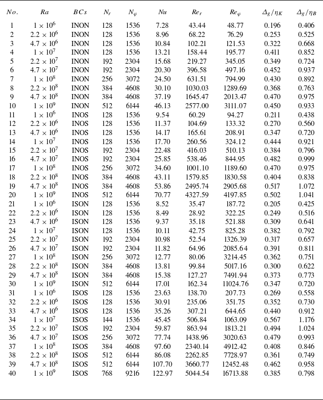
 η=0.5,Pr=4.3
 Ro−1=20
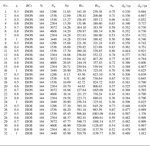
 Ra=107,Pr=4.3
 Ro−1=20
 η=0.9
 η=1
 Lx/Lz=10


