





1. Introduction
Whether incentives alter attention has become a key question for a growing literature on the role of cognition in economics (e.g.,Bronchetti et al., Reference Bronchetti, Kessler, Magenheim, Taubinsky and Zwick2023).Footnote 1 An important aspect of this question is whether perceptual limits (“capacities” or “constraints”) are exogenously fixed or if perception can be improved when desired. For example, in the rational inattention literature, Sims (Reference Sims2003) assumes the bounds on attention are fixed, while Matejka and McKay (Reference Matejka and McKay2015) assume the bounds are elastic and can be loosened at a cost. In the efficient coding literature, Woodford (Reference Woodford2012) provides versions of optimal encoding with both fixed bounds and elastic bounds.Footnote 2 Whether or not perceptual capacity is fixed or variable has substantial implications for the economic impact of bounded cognition. Most importantly, if perceptual constraints are exogenously fixed, then changes in incentives will not alter the extent of attention, only how individuals decide to allocate their scarce attention.
The question of whether incentives impact the extent of attention also relates to an ongoing debate about whether incentivization matters in experiments. Various reasons have been given for incentivizing experiments (e.g., Plott, Reference Plott1986; Smith, Reference Smith1991), but most experiments on perception and attention in the psychology literature do not incentivize performance; implicitly treating incentives as irrelevant to cognition. However, this assumption has been challenged by papers showing the impact of rewards on visual perception in the psychology literature on psychometrics (e.g., Pessoa and Engelmann, Reference Pessoa and Engelmann2010).
We offer a method for answering the question of whether perceptual capacity is exogenously fixed, and hence whether incentives impact the extent of attention, by providing a sharp test of capacity-constrained learning models. In this class of models, a decision-maker can learn about the true state only through an exogenously fixed set of feasible learning strategies. Incentive changes can affect which feasible strategy they choose, but cannot expand the underlying set of learning strategies that is available to be used. Because feasibility is imposed as a fixed constraint on learning rather than a choice variable, this model class includes settings with exogenous perceptual limits, such as fixed-capacity rational inattention (Sims, Reference Sims2003) and efficient coding (Woodford, Reference Woodford2012). Our contribution is to provide a test that directly addresses the questions above: because incentives can only expand attention if perceptual capacity is elastic, violations of our test can be interpreted as evidence that incentives matter for attention and perception.
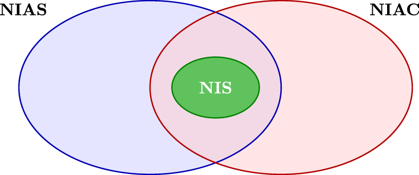
We show that a single condition, No Improving (Action or Attention) Switches (NIS), is both necessary and sufficient for choices to be consistent with models of capacity-constrained learning. NIS sharpens the No Improving Action Switches (NIAS) condition, which requires optimal actions given information (Caplin and Martin, Reference Caplin and Martin2015), and the No Improving Attention Cycles (NIAC) condition, which rules out profitable reallocations of attention across problems (Caplin and Dean, Reference Caplin and Dean2015) Figure 1 illustrates the relationship between NIS, NIAS, and NIAC. In words, NIS states that wholesale switches of attention or actions, both within and across decision problems, should not improve utility. Incentives thus enter our framework not as an auxiliary consideration but as the central empirical tool: when NIS fails, it is because incentives induce systematic reallocations of attention that would not occur if perceptual capacity were fixed.
Relationship between NIS and existing conditions (NIAS and NIAC)

We apply our test of capacity-constrained learning to data from three existing experiments that vary the payoffs to being correct in visual perception tasks. We first look at experiments 1.2 and 2.2 of Dean and Neligh (Reference Dean and Neligh2023), which vary the reward to correctly guessing the state in two tasks: the number of colored balls in a visual display (1.2) and the number of correct equations (2.2). Using the aggregated choices of participants, we find that NIAS and NIAC are satisfied for both experiments. However, NIS fails in both experiments, and the failure is statistically significant in Experiment 1.2 ( $p \lt 0.01$).Footnote 3 Importantly, NIS fails in a systematic way in both experiments: switching attention in the direction of higher incentives (switching to the attention used when incentives were higher) always leads to improvements in expected utility.
Next, we reexamine the data from the experiment of Caplin et al. (Reference Caplin, Csaba, Leahy and Nov2020), which varies the payoff for correctly guessing which shape appears the most frequently. We find that NIAS is satisfied for all four difficulty levels of the task, but that NIS is not satisfied for any of the difficulty levels (statistically significant for all four).
Finally, we re-analyze the data from the experiment of Dewan and Neligh (Reference Dewan and Neligh2020), which varies the payoffs using two possible prize sizes ($10 and $20). For the first task, correctly guessing the number of balls in a display, we again find that NIAS and NIAC are satisfied for both prize sizes, but NIS fails for both (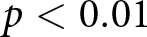 $p \lt 0.01$ for each prize size). As in the other experiments, we find that for a given prize size, switches of attention in the direction of higher incentives always lead to improvements in expected utility.
However, for the second task of Dewan and Neligh (Reference Dewan and Neligh2020), which requires participants to judge the degree of an angle, we do not find strong evidence that NIS fails for either of the prize sizes ( $p=0.22$ and
 $p=0.86$). In addition, unlike the other experiments, switches of attention in the direction of higher incentives (for a given prize size) often do not lead to improvements in expected utility.
These results suggest that certain task factors might dictate the suitability of capacity-constrained learning. Specifically, this model class might be more appropriate for tasks that are not responsive to additional effort.Footnote 4 This can occur because (1) even at low incentives, an individual chooses to exert enough effort to reach their perceptual limit, and (2) additional effort would not meaningfully improve perception beyond this limit. This combination of forces causes individuals to reach the same level of “irreducible uncertainty” at all levels of incentives. Another possibility is that uncertainty could actually be reduced further, but individuals choose not to spend the additional effort required to reduce it further at standard incentive levels. Determining what class of perceptual and judgment tasks is insensitive to incentive changes is an open area for experimental work and will be central to assessing when models of capacity-constrained learning are suitable for environments with changing incentives.
Our paper contributes to a growing literature on testing economic models of cognition (e.g., Almog and Martin, Reference Almog and Martin2024; Almog et al., Reference Almog, Gauriot, Page and Martin2024 Caplin et al., Reference Caplin, Csaba, Leahy and Nov2020; de Clippel and Rozen, Reference de Clippel and Rozen2020; Dewan and Neligh, Reference Dewan and Neligh2020; Dean and Neligh, Reference Dean and Neligh2023). This literature includes tests of models of costly attention and rational inattention, in which cognition is treated as an endogenous, resource-constrained input into choice (see Shenhav et al., Reference Shenhav, Musslick, Lieder, Kool, Griffiths, Cohen and Botvinick2017; Gabaix, Reference Gabaix, Bernheim, DellaVigna and Laibson2019; Maćkowiak et al., Reference Maćkowiak, Matějka and Wiederholt2023 for reviews). It also includes experimental and psychometric approaches that use controlled tasks to identify and test restrictions implied by attention-based models (e.g., Dean and Neligh, Reference Dean and Neligh2023; Caplin et al., Reference Caplin, Csaba, Leahy and Nov2020; Ambuehl et al., Reference Ambuehl, Ockenfels and Stewart2025). Our primary contribution to this literature is to examine the consistency of human choices with capacity-constrained learning models.
Related work emphasizes that economic behavior can also depend on the choice of attention environments and attention-improving tools, and develops theory-driven tests using willingness-to-pay and incentive variation in such settings (e.g., Bronchetti et al., Reference Bronchetti, Kessler, Magenheim, Taubinsky and Zwick2023; Gabaix, Reference Gabaix2014; De Oliveira et al., Reference De Oliveira, Denti, Mihm and Ozbek2017). Our primary contribution within this agenda is to provide and implement a sharp revealed-preference test for whether observed behavior is consistent with capacity-constrained learning, thereby isolating when incentive changes can be rationalized by reallocating fixed attention versus requiring an expansion of attentional capacity. This positions our test as not only the first general test of capacity-constrained learning, but also as a novel way of adjudicating the long-standing debate about whether incentives alter the extent of human attention.
Our test also has implications for non-human learners. Caplin et al. (Reference Caplin, Martin and Marx2025) apply our test to the predictions of a state-of-the-art machine learning algorithm that is trained to identify pneumonia from chest x-rays. In the context of machine learning, capacity-constrained learning aligns with standard notions of how a machine learns, as this model class can be interpreted as the machine choosing among a feasible set of mathematical operations to best match the incentives provided by its loss function. Echoing the results in this paper, Caplin et al. (Reference Caplin, Martin and Marx2025) find that a state-of-the-art machine learning algorithm violates NIS but not NIAS or NIAC in an experiment in which the loss function used to train the algorithm is varied.
The rest of the paper is as follows. Section 2 introduces NIS, our test of capacity-constrained learning. Section 3 proposes approaches to measuring the extent of NIS violations and the statistical testing of NIS. Section 4 provides the results of testing NIS using the data from existing experiments. Section 5 concludes.
2. Our test of capacity-constrained learning
In a capacity-constrained learning model, the decision-maker faces an objectively defined but uncertain state and must choose an action whose payoff depends on that state. Before acting, the decision-maker may acquire information, but only via a capacity constraint that is represented as a fixed feasibility set: a collection of learning strategies the person is capable of using. A learning strategy can be understood as a rule that determines what noisy evidence the person can generate about the state and therefore what posterior beliefs they can end up holding.
Capacity-constrained learning imposes three key requirements. First, the set of learning strategies available to the decision-maker is the same across decision problems and does not change with the payoff scale. Second, in each decision problem, the decision-maker selects whichever feasible learning strategy yields the highest expected payoff for that problem. Finally, once a signal is realized, the decision-maker updates beliefs in a Bayes-consistent way and chooses an action that is optimal given those beliefs.
Consider a researcher who wants to determine if a decision-maker chose in line with capacity-constrained learning, but does not observe the information actually obtained by the decision-maker, their beliefs, or their attention. The following sections introduce a test the researcher can use to answer this question. A more precise definition of capacity-constrained learning and our representation result are provided in the Online Appendix.
2.1. Preliminaries
This section introduces the objects a researcher needs in order to apply our test using observed choice data. The researcher observes a finite set of experimental decision problems, each defined by a known set of possible states, a set of available actions, and a payoff rule that rewards actions as a function of the realized state. In particular, there is a finite set of possible states of the world  $\omega\in\Omega$ distributed according to an objective prior μ,Footnote 5 a finite global set of actions
 $a \in \mathcal{A}$ with
 $| \mathcal{A} | \geq 2$, and a finite global set
 $x \in X$ of prize specifications, with realizations
 $x(a,\omega)$ that depend on the realized state and action in a way known by the researcher. Thus, a decision problem
 $i \in D$ consists of an action set
 $A_i \subseteq \mathcal{A}$ and a prize specification
 $x_i \in X$.Footnote 6
For example, Experiment 1.2 of Dean and Neligh (Reference Dean and Neligh2023) (DN23 hereafter) has two equally likely states: out of the 100 balls presented on the screen, there can either be 49 red balls and 51 blue balls or 51 red balls and 49 blue balls (labeled states  $\omega_1$ and
 $\omega_2$, respectively). The global set of actions
 $\mathcal{A}=\{a_1,a_2\}$ is common across decision problems, and individuals are incentivized to match actions and states (choosing
 $a_1$ in state
 $\omega_1$ and
 $a_2$ in state
 $\omega_2$) according to a varying prize specification such that a correct guess leads to either 5, 40, 70, or 95 probability points (the probability of receiving a fixed cash amount) while an incorrect guess yields 0 probability points. This structure is typical of many experimental designs: the states and actions are fixed across treatments, while incentives vary. To summarize, the set of decision problems
 $i \in \{1,2,3,4 \}$ consists of common states and actions yielding varying probability point prizes, which are known to correspond to actions and states as follows:
 \begin{align*}
\Omega & = \{\omega_1,\omega_2\},\qquad A_i = \{a_1,a_2\},\\
x_i(a,\omega) & =
\begin{array}{c@{\;}c} & \begin{array}{cc} \omega_1 & \omega_2 \end{array} \\[-2pt]
\begin{array}{c}
a_1\\
a_2\end{array} & \left( \begin{array}{cc}
p_i & 0\\
0 & p_i
\end{array}
\right)
\end{array} \qquad
\text{where}\quad
p_i =
\begin{cases}
5 & \text{for } i=1,\\
40 & \text{for } i=2,\\
70 & \text{for } i=3,\\
95 & \text{for } i=4.
\end{cases}
\end{align*}
The decision-maker (DM) is assumed to have a utility function  $u$ over prizes. In all the experiments we examine, prizes take the form of “probability points” which directly determine the chances of receiving a fixed monetary amount. Under the expected utility framework, the utility of a prize that offers a given number of probability points is linear in the number of probability points, because these points scale the probability of a fixed outcome rather than the outcome itself. If we additionally assume that receiving cash yields more utility than not receiving it, then the utility of the prize is also strictly increasing in the number of probability points. Without loss of generality, we can normalize the utility of receiving the cash prize to 100 and not receiving the cash to 0, in which case the utility of the probability point prize is point identified: the utility of
 $p$ probability points is exactly
 $p$.
The data required for our test are the joint frequencies with which subjects choose each action in each realized state, separately for each decision problem. We summarize these frequencies as state-dependent stochastic choice (SDSC) matrices  $P_i (a,\omega)$. These include, for each decision problem
 $i \in D$, the joint distribution of actions and states
 $P_i (a,\omega)$ for all
 $a\in A_i$ and
 $\omega\in\Omega$. We denote as
 $P$ the collection of
 $P_{i}$ for every decision problem
 $i\in D$.
For example, in Experiment 1.2 of DN23, the set of aggregate (across-subject) joint distributions  $P$ is:
 \begin{align*}
P_1 & =
\begin{array}{c}
\\[-1.2em]
a_1\\
a_2
\end{array}
\left(
\begin{array}{cc}
\omega_1 & \omega_2\\
0.37 & 0.20\\
0.13 & 0.30
\end{array}
\right),
\qquad
P_2 =
\begin{array}{c}
\\[-1.2em]
a_1\\
a_2
\end{array}
\left(
\begin{array}{cc}
\omega_1 & \omega_2\\
0.38 & 0.17\\
0.12 & 0.33
\end{array}
\right),\\
P_3 & =
\begin{array}{c}
\\[-1.2em]
a_1\\
a_2
\end{array}
\left(
\begin{array}{cc}
\omega_1 & \omega_2\\
0.39 & 0.17\\
0.11 & 0.33
\end{array}
\right),
\qquad
P_4 =
\begin{array}{c}
\\[-1.2em]
a_1\\
a_2
\end{array}
\left(
\begin{array}{cc}
\omega_1 & \omega_2\\
0.39 & 0.14\\
0.11 & 0.36
\end{array}
\right).
\end{align*}
In summary, to apply our test, an experimentalist needs only (i) observed choices in each state and (ii) the payoff rule linking actions and states.
2.2. NIS: capacity-constrained learning
The condition for a collection of SDSC data  $P$ to be consistent with capacity-constrained learning is given below. Importantly, our test relies only on observed choices and known payoff rules.
Condition 1 (No Improving (Action or Attention) Switches (NIS)).
Utility function  $u$ satisfies NIS for
 $P$ if and only if for any set of decision problems
 $i,j \in D$,
 \begin{equation}
\sum_{a\in A_i} \sum_{\omega\in\Omega} P_{i}(a,\omega) u(x_i(a,\omega)) \geq
\sum_{a\in A_j} \max_{\hat{a}\in A_i} \sum_{\omega\in\Omega} P_{j}(a,\omega) u(x_i (\hat{a},\omega))
\end{equation}
In words, this condition states that wholesale switches of attention and actions should not improve utility according to the baseline prize specification. Intuitively, NIS states that reusing any feasible pattern of learning observed in one decision problem should not improve expected utility in another with the same payoff rule. NIS involves both checks between decision problems (when  $i \neq j$), where both actions and choice probabilities can change, and checks “within” each decision problem (when
 $i = j$), where only actions can change. Thus, NIS involves checking
 $N^2$ inequalities. The Online Appendix describes how NIS relates to two existing tests of Bayesian learning (NIAS and NIAC).
2.2.1. Example: Dean and Neligh (2023)
To illustrate NIS we turn to the decision problems, prizes, and aggregate (rounded) SDSC data from Experiment 1.2 of DN23, which are given in Section 2.1. Restricting for simplicity to just the first two decision problems ( $1,2$) in which the number of probability points was 5 and 40 respectively, the data
 $P$ is:
 \begin{equation*}
P_1 =
\begin{array}{c@{\;}c}
&
\begin{array}{cc}
\omega_1 & \omega_2
\end{array}
\\[-2pt]
\begin{array}{c}
a_1\\
a_2
\end{array}
&
\left(
\begin{array}{cc}
0.37 & 0.20\\
0.13 & 0.30
\end{array}
\right)
\end{array}
\qquad
P_2 =
\begin{array}{c@{\;}c}
&
\begin{array}{cc}
\omega_1 & \omega_2
\end{array}
\\[-2pt]
\begin{array}{c}
a_1\\
a_2
\end{array}
&
\left(
\begin{array}{cc}
0.38 & 0.17\\
0.12 & 0.33
\end{array}
\right)
\end{array}
\end{equation*}
The NIS condition makes four comparisons: switches of actions within (decision) problem  $1$, switches of actions within problem
 $2$, switches of choice probabilities and actions from problem
 $1$ to
 $2$, and switches of choice probabilities and actions from problem
 $2$ to
 $1$. Concretely, the test checks whether outcomes could be improved by either reassigning actions within a given problem, or by reusing the learning reflected in choices under one problem and applying it to the other problem, in both directions. In this case, switches of choice probabilities from problem
 $1$ to
 $2$ generate a violation of NIS, which we will show below. Practically, this means that the pattern of choices in problem 2 (the problem that is identical to problem 1 except for in terms of prize) reveals a feasible way of learning and applying that same learning to problem 1 would improve expected utility. Under fixed feasibility, such an improvement should not be possible, so NIS is violated.
As a first step, we compute the expected utility implied by the observed choice frequencies in decision problem 1, treating these frequencies as revealing how the subject learned about the state. The value of the data in decision problem  $1$ is
 \begin{align*}
& \underbrace{P_{1}(a_1, \omega_1) u(x_1 (a_1, \omega_1))}_{0.37 \times 5} + \underbrace{P_{1}(a_1, \omega_2) u(x_1 (a_1, \omega_2))}_{0.20 \times 0} \\ &+ \underbrace{P_{1}(a_2, \omega_1) u(x_1(a_2, \omega_1))}_{0.13 \times 0} + \underbrace{P_{1}(a_2, \omega_2) u(x_1 (a_2, \omega_2))}_{0.30 \times 5}
\\
&= 3.35.
\end{align*}
We next ask whether the learning revealed in decision problem 2 could have been reused in decision problem 1. To do this, we evaluate the choice frequencies from problem 2 using the payoffs and optimal actions from problem 1, which results in
 \begin{align*}
& \underbrace{P_{2}(a_1, \omega_1) u(x_1 (a_1, \omega_1))}_{0.38 \times 5} + \underbrace{P_{2}(a_1, \omega_2) u(x_1 (a_1, \omega_2))}_{0.17 \times 0} \\ &+ \underbrace{P_{2}(a_2, \omega_1) u(x_1(a_2, \omega_1))}_{0.12 \times 0} + \underbrace{P_{2}(a_2, \omega_2) u(x_1 (a_2, \omega_2))}_{0.33 \times 5}
\\
&= 3.55.
\end{align*}
Because the optimal actions remain the same and choice probabilities on the diagonal increase, switching results in a net gain of utility ( $0.21$). Thus, there would have been an improving switch in utility by using the implied learning in decision problem
 $2$ in decision problem
 $1$. As a result, NIS is not satisfied for this data. Since the existing experiments vary payoffs, NIS effectively tests whether attention expands in response to incentives, and NIS failing effectively means the failure of the capacity-constrained learning model.
3. Taking NIS to data
For the experiments that we study, NIS makes the stringent prediction that the percentage correct has to be identical across treatments. When evaluating whether data are consistent with this prediction, two distinct questions arise. The first is a question of magnitude: if a violation occurs, how large is it? The second is a question of statistical inference: given that we observe only a finite sample, can we confidently conclude that the population violates NIS? A violation can be large but statistically insignificant (if the sample is small or noisy), or small but statistically significant (if the sample is large enough to detect minor deviations). We address both questions in turn. Section 3.1 proposes two Improvability Indices (IDI and IEI) that quantify the economic magnitude of NIS violations. Section 3.2 develops a statistical test whose  $p$-value quantifies our confidence that observed violations are not due to sampling noise.
3.1. Improvability Indices
A known challenge in testing axioms with choice data is that axioms are either satisfied or not, which is fairly stark. Instead, when they fail it might be useful to know the extent of the failure.
In the same spirit as a literature that measures the extent of violations of rationality for deterministic models of decision-making (Afriat, Reference Afriat1973; Varian, Reference Varian1991; Echenique et al., Reference Echenique, Lee and Shum2011; Apesteguia and Ballester, Reference Apesteguia and Ballester2015; Dean and Martin, Reference Dean and Martin2016), we propose two measures for the extent of violations of rationality for stochastic models of decision-making.Footnote 7 The measures are stated here for NIS, but could be extended to cover other conditions, such as NIAS and NIAC.
The first measure we propose is the Improvability Difference Index (IDI). This index indicates the largest difference between the actual expected utility obtained in a decision problem and what could be achieved by switching actions and attention. To aid comparability across decision problems, it is normalized by the maximum achievable expected utility within a decision problem, so takes a value between 0 and 1.Footnote 8
Technically, IDI is the larger of 0 and the (normalized) difference between the expected utility under the chosen attention in a decision problem (the left-hand side of the NIS condition 1) and the expected utility from using the attention chosen in a different decision problem (the right-hand side of the NIS condition 1):
 \begin{equation}
\max_{i,j \in D}{
\frac{
\sum_{a\in A_j} \max_{\hat{a}\in A_i} \sum_{\omega\in\Omega} P_{j}(a,\omega) u(x_i(\hat{a},\omega))-\sum_{a\in A_i} \sum_{\omega\in\Omega} P_{i}(a,\omega) u(x_i(a,\omega))
}{
\sum_{\omega\in\Omega} \max_{\hat{a}\in A_i} \mu(\omega) u(x_i(\hat{a},\omega))}
}
\end{equation}
NIS passes if and only if IDI is 0, and higher values of IDI indicate that NIS is violated by more of the maximum expected utility.
Second, we propose the Improvability Efficiency Index (IEI), which is the largest fraction of expected utility on the right-hand side of the NIS condition (the expected utility from using the attention chosen in a different decision problem) that can be retained without exceeding the left-hand side of the NIS condition (expected utility obtained in a decision problem). Technically, we calculate IEI by finding the largest value of  $\epsilon\in[0,1]$ such that the following inequality holds for all sets of decision problems
 $i,j \in D$:
 \begin{equation}
\sum_{a\in A_i} \sum_{\omega\in\Omega} P_{i}(a,\omega) u(x_i(a,\omega)) \geq \epsilon
\sum_{a\in A_j} \max_{\hat{a}\in A_i} \sum_{\omega\in\Omega} P_{j}(a,\omega) u(x_i(\hat{a},\omega))
\end{equation}
Clearly, NIS passes if and only if IEI is 1, and lower values of IEI indicate that a higher fraction of expected utility has to be shaved off of the RHS to make NIS pass. This can be interpreted as the utility that has to be shaved from every state on the RHS to make NIS pass.Footnote 9
The closest measure to IEI is the Critical Cost Efficiency Index (CCEI) (Afriat, Reference Afriat1973), which measures the budget set reduction necessary for the Generalized Axiom of Revealed Preference (GARP) to be satisfied for deterministic choice. Like IDI and IEI, the CCEI measures the largest violation in a set of choice data.
3.2. Statistical testing
NIS is a property of the population-level joint distribution  $P$ of states and choices, which is not directly observable in experimental data. Instead, experiments generate a finite sample drawn from
 $P$, inducing an empirical distribution
 $\hat{P}$. This gap creates the need for statistical testing.
A number of methods have been used to evaluate the statistical significance of NIAS and NIAC. For example, in Dewan and Neligh (Reference Dewan and Neligh2020), NIAS is tested using bootstrapping. If no more than 5% of samples for each action for a given subject fail, then that subject fails to reject NIAS. In Dewan and Neligh (Reference Dewan and Neligh2020), NIAC is tested using regression. They run a linear weighted least squares regression of correctness on incentive level and then perform a one-sided  $t$-test on the coefficient of the incentive level.
This paper evaluates significance using the Wald test. This test calculates the distance between our estimated parameter values  $ P(a, \omega) $ across actions and states, and the set of values that satisfy the null hypothesis of NIS, and then compares it with a
 $\chi^2$ distribution to determine the
 $p$-value. A key step in the Wald test is calculating the covariance matrix of the difference between the right-hand side and the left-hand side of the NIS inequality, which is
 \begin{equation}
\sum_{a \in A_i} \sum_{\omega \in \Omega} P_{i}(a, \omega) u(x_i (a, \omega)) -
\sum_{a \in A_j} \max_{\hat{a} \in A_i} \sum_{\omega \in \Omega} P_{j}(a, \omega) u(x_i (\hat{a}, \omega)).
\end{equation}
This is achieved using the Delta Method, which is also applied in Dean and Neligh (Reference Dean and Neligh2023) to test NIAC in Experiment 1.2. This approach assumes only the asymptotic normality of the estimators. For example, in the common case where actions are binary, we observe  $\hat{P}(a | \omega)$, which represents a draw from a binomial distribution. This binomial distribution has a mean of
 $ P(a | \omega) $, with the number of trials determined by the frequency of state
 $\omega$. With a large number of trials, this distribution is approximately normal, validating the assumption. Additionally, the Delta Method relies on the first-order approximation of the Taylor expansion of expression (4). However, since in our case the expression is a linear function of
 $\hat{P}(a | \omega)$, the first-order approximation of the Taylor expansion is the exact value. This is another reason the Delta Method is especially suitable for our case.
In both Dean and Neligh (Reference Dean and Neligh2023) and Caplin et al. (Reference Caplin, Csaba, Leahy and Nov2020), the prizes, states, and action spaces are all binary and the states are ex ante equally likely.Footnote 10 In that case, the NIS expression (4) reduces to
 \begin{equation*}
P_{i}(a_1 | \omega_1) + P_{i}(a_2 | \omega_2) -
\max_{\hat{a} \in \{a_1, a_2\}} \big\{P_{j}(\hat{a} | \omega_1) + (1 - P_{j}(\hat{a} | \omega_2))\big\} \geq 0
\end{equation*}
for all  $i, j \in D $. This implies
 \begin{equation}
P_{i}(a_1 | \omega_1) + P_{i}(a_2 | \omega_2) -
\max_{\hat{a} \in \{a_1, a_2\}} \big\{P_{j}(\hat{a} | \omega_1) + (1 - P_{j}(\hat{a} | \omega_2))\big\} = 0
\end{equation}
for all  $i \neq j \in D$, and
 \begin{equation}
P_{i}(a_1 | \omega_1) + P_{i}(a_2 | \omega_2) -
P_{i}(a_1 | \omega_2) - P_{i}(a_2 | \omega_1) \geq 0
\end{equation}
for all  $i \in D $. As discussed in the Online Appendix, the latter condition (6) within decision problem is equivalent to NIAS in the restricted setting. Therefore, assuming that NIAS is satisfied and plugging into the preceding equation (5) yields the implication that:
 \begin{equation}
P_i (a_1 | \omega_1) + P_i (a_2 | \omega_2)
=
P_j (a_1 | \omega_1) + P_j (a_2 | \omega_2)
\end{equation}
for all  $i,j \in D$. Equation (7) represents a subset of the NIS inequalities in our restricted setting, taking NIAS as given. Intuitively, it requires that accuracy be independent of incentives.Footnote 11 This is easily tested using an off-the-shelf Wald test for multivariate equality. If this relaxed test is rejected, then so is the more stringent NIS condition nesting NIAS. Otherwise, it is possible to test the full set of NIS conditions (5) and (6) using a Wald test for mixed joint hypotheses with equalities and inequalities (Kodde and Palm, Reference Kodde and Palm1986). In what follows, we focus on the simplified implication (7), given that NIAS is typically satisfied pointwise.Footnote 12
4. Existing experiments
In this section, we re-examine the data from existing experiments of Dean and Neligh (Reference Dean and Neligh2023), Caplin et al. (Reference Caplin, Csaba, Leahy and Nov2020), and Dewan and Neligh (Reference Dewan and Neligh2020). We focus on these three studies because they jointly satisfy the criteria necessary to implement our test cleanly. First, each study employs a match-the-state structure with a well-defined, finite state space: binary-state environments in DN23 and CCLN, and a five-state environment in DN20. Second, each varies incentives across multiple levels while holding the action set and payoff mapping fixed, which is precisely the variation NIS exploits. Third, each provides the joint distribution of realized states and chosen actions; the minimal data requirement for our test. Finally, all three studies have publicly available datasets and use samples large enough to support statistical inference. Together, these features make them well-suited for the first empirical application of NIS.
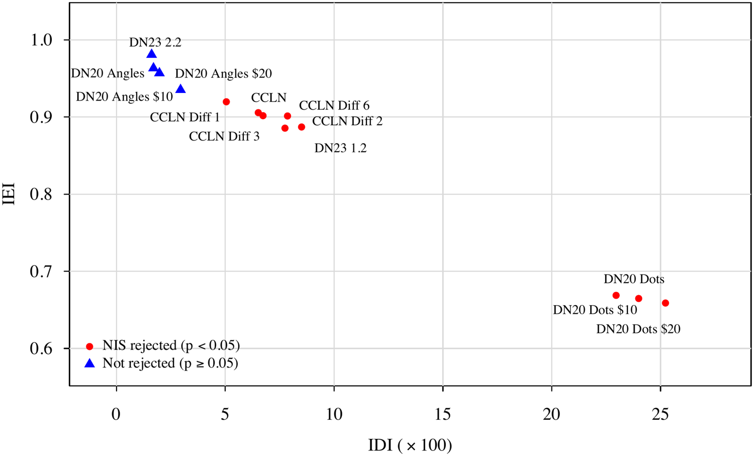
Table 1 and Figure 2 provide an overview of the analysis. The empirical results are reached in two steps. First, for each dataset we spell out the inequalities implied by NIS: these specify how accuracy should compare across incentive conditions if perceptual capacity is fixed. Second, we test these predictions against the observed data. A rejection of NIS occurs whenever the observed pattern of accuracies contradicts these inequalities. That is, when different incentives yield systematically and significantly different accuracy than predicted under NIS. With this structure in place, the reader can interpret each set of results as a direct test of the NIS inequalities in the context of the relevant experiment. Therefore, when Table 1 and Figure 2 specify that NIS is rejected, it is rejecting precisely the hypothesis that a change in incentives did not alter the capacity of participants in this experiment. As Table 1 and Figure 2 show, NIS is rejected in most tasks we study, including DN23’s ball-counting task, CCLN (shapes), and DN20 (dots). However, NIS is not rejected in DN20’s angle-judgment task, suggesting that this type of perceptual problem is less responsive to incentives. This contrast highlights the main takeaway: while incentives systematically expand attention in many standard perceptual settings, some tasks exhibit limits that are insensitive to payoff variation. Figure 2 further shows that (i) there is a negative relationship between IEI and IDI and (ii) IEI/IDI is strictly smaller/larger for tasks in which NIS is rejected.Footnote 13
IDI vs. IEI across experiments. Color/shape indicates whether the NIS test is rejected at  $\alpha=0.05$

Figure 2 Long description
The scatter plot illustrates the relationship between IEI and IDI times 100. The horizontal axis represents IDI times 100 and the vertical axis represents IEI. Data points are marked with red circles for NIS rejected and blue triangles for not rejected at a significance level of p less than 0.05. A dense cluster of points is visible at low IDI values with higher IEI, while a smaller set of points appears at higher IDI values with lower IEI. Notable labeled points include DN23 2.2, DN20 Angles $10, DN20 Angles $20, CCLN and DN20 Dots. The plot suggests a general trend where IEI decreases as IDI increases, highlighting the impact of NIS rejection across different experiments.
Summary of results for aggregate data from all experiments

Table 1 Long description
Rows list experiments and columns report number of incentive levels, NIAS and NIAC pass or fail status, whether NIS was rejected at alpha 0.05, the NIS joint p-value, IDI, IEI, and sample size N. DN23 1.2 has 4 incentive levels, NIAS Pass, NIAC Pass, NIS rejected Yes, joint p-value less than 0.01, IDI 0.09, IEI 0.89, N 10400. DN23 2.2 has 2 incentive levels, NIAS Pass, NIAC Pass, NIS rejected No, joint p-value 0.38, IDI 0.02, IEI 0.98, N 5500. CCLN has 6 incentive levels, NIAS Pass, NIAC Fail, NIS rejected Yes, joint p-value less than 0.01, IDI 0.07, IEI 0.91, N 26048; its Difficulty 1, 2, 3, and 6 rows each show NIAS Pass and NIAC Fail with NIS rejected Yes, joint p-values 0.04, less than 0.01, 0.01, and less than 0.01, IDI values 0.05, 0.08, 0.07, and 0.08, IEI values 0.92, 0.89, 0.90, and 0.90, and N values 7136, 6240, 6656, and 6016. DN20 Dots has 4 incentive levels, NIAS Pass, NIAC Pass, NIS rejected Yes, joint p-value less than 0.01, IDI 0.24, IEI 0.66, N 8100; Dots 10 and Dots 20 also show Pass for NIAS and NIAC with NIS rejected Yes, joint p-values less than 0.01, IDI 0.23 and 0.25, IEI 0.67 and 0.66, and N 4100 and 4000. DN20 Angles has 4 incentive levels, NIAS Fail, NIAC Fail, NIS rejected No, joint p-value 0.58, IDI 0.02, IEI 0.96, N 8100; Angles 10 matches Fail and Fail with NIS rejected No, joint p-value 0.22, IDI 0.03, IEI 0.94, N 4100, while Angles 20 shows NIAS Pass and NIAC Fail with NIS rejected No, joint p-value 0.86, IDI 0.02, IEI 0.96, N 4000.
4.1. Dean and Neligh (2023): dots & equations
4.1.1. Design
As described in Section 2.1, participants in Experiment 1.2 of Dean and Neligh (Reference Dean and Neligh2023) (DN23 hereafter) face a choice between two actions ( $a$ or
 $b$) with two equally likely states (represented by 49 blue and 51 red balls (R) or 49 red and 51 blue balls (B)). When the state is R (more red balls), the “correct” action is
 $a$, and when the state is B (more blue balls), the correct action is
 $b$. In our notation, this is analogous to an incentive to choose actions to match the state, that is, choosing
 $a_k$ when the state is
 $\omega_k$ for
 $k = R,B$. For a randomly selected choice, participants are given probability points (for a prize of $40) if they chose the correct action and the number of probability points varies across decision problems: either 5, 40, 70, or 95 points (4 incentive levels), as can be seen in Table 1. Fifty-two participants face 50 repetitions of each of these four decision problems. Experiment 2.2 has a similar design, but the 55 subjects face seven equations instead of dots with two states of the world being either three or four of the seven equations being correct. The incentive structure remained broadly the same with only the 5 probability points payment and the 95 probability points payment (2 incentive levels, as can be seen in Table 1).
4.1.2. Results
As can be inferred from the joint distribution matrices presented in Section 2.1, subjects improve their accuracy in the direction of increasing incentives, that is, using the higher incentive-level information structure for a lower incentive-level problem. Formally, we test pairwise NIS inequalities for each ordered pair of incentive levels. With four incentive levels, there are sixteen such ordered pairs in total: six in the direction of increasing incentives, six in the direction of decreasing incentives, and four within the same incentive level. We find that all six comparisons in the direction of increasing incentives yield an improving switch of attention, while none of the remaining comparisons do. The magnitude of these violations in aggregate leads us to reject NIS with a joint p-value less than  $0.01$ (see Table 1). Table 2 unpacks these results using the aggregate data from DN23 Experiment 1.2 for each incentive level pair, with
 $p$-values corresponding to the one-sided null hypothesis that the NIS RHS (performance given capacity at the higher incentive level) is no greater than the LHS (performance given capacity at the lower incentive level) for each incentive-level switch. These violations of NIS arise systematically because higher incentives lead subjects to deploy more attention, generating accuracy gains inconsistent with fixed-capacity models. Put differently, the test fails here not at random but precisely where incentives are raised, highlighting their role in shaping perceptual effort
NIS inequalities in direction of increasing incentives (aggregate data from experiment 1.2 of DN23)

Table 2 Long description
Rows compare two incentive levels labeled, Lower and, Higher, and report NIS LHS, NIS RHS, whether, NIS inequality fails, and a p-value. For Lower 5 and Higher 40, NIS LHS is 3.34 and NIS RHS is 3.56, with failure marked Yes and p-value 0.03. For Lower 5 and Higher 70, NIS LHS is 3.34 and NIS RHS is 3.60, with Yes and p-value 0.02. For Lower 5 and Higher 95, NIS LHS is 3.34 and NIS RHS is 3.77, with Yes and p-value less than 0.01. For Lower 40 and Higher 70, NIS LHS is 28.46 and NIS RHS is 28.84, with Yes and p-value 0.33. For Lower 40 and Higher 95, NIS LHS is 28.46 and NIS RHS is 30.12, with Yes and p-value 0.05. For Lower 70 and Higher 95, NIS LHS is 50.46 and NIS RHS is 52.71, with Yes and p-value 0.11.
If we take the RHS to be the best possible result that can be achieved with the subject’s current level of learning and LHS to be the actual level achieved, the difference between them can be used to calculate the Improvability Index (IDI), as explained in Section 3.1. Our measure of IDI is the maximum improvement over all decision problems, normalized by the best possible outcome in each decision problem. The largest normalized improvement relative to baseline comes from the test comparing the performance at the lowest level of incentives (5) with the learning structure from the highest level of incentives (95). The improvement is 0.43 probability points, which corresponds to an increase in 8.5% of the maximum that could be achieved in that decision problem.
The results from Experiment 2.2 of DN23 show a similar pattern: RHS  $ \gt $ LHS in Table 3, indicating that switching attention in the direction of increasing incentives would improve expected utility. However, the violation is small in magnitude (IDI = 1.6%) and statistically insignificant (
 $p = 0.19$), so we cannot reject the null hypothesis that NIS holds in the population. Two factors likely explain this. First, Experiment 2.2 has only two incentive levels, yielding fewer inequalities to test and limiting statistical power. Second, accuracy exceeds 80% even at the lowest incentive level, leaving little room for incentives to expand attention further; a ceiling effect that dampens the scope for detectable violations.
NIS inequalities in direction of increasing incentives (aggregate data from experiment 2.2 of DN23)

Table 3 Long description
Columns are DP1, DP2, LHS, RHS, NIS inequality fails?, and p-value. One row reports DP1 5 and DP2 95. For this row, LHS is 4.13 and RHS is 4.21. The column, NIS inequality fails?, is Yes. The p-value is 0.19.
4.2. Caplin, Csaba, Leahy, and Nov (2020): polygons
4.2.1. Design
In this experimental task, subjects are shown 24 geometric objects at once. Each one of these objects is a polygon that has either 7, 8, 9, or 10 sides. Subjects are asked to make a binary decision indicating whether they believe that there are more 7-sided polygons (action “heptagon”) or 9-sided polygons (action “nonagon”). Again, in our notation, this is analogous to an incentive to choose the action to match the state, that is, choosing  $a_k$ when the state is
 $\omega_k$ for
 $k = 7,9$. The number of 7- and 9-sided polygons thus determines the difficulty level of the task: the smaller the difference, the harder the task. Caplin et al. (Reference Caplin, Csaba, Leahy and Nov2020) (CCLN hereafter) vary between participants the difference to be either 1, 2, 3, or 6 (the difficulty level is fixed for a given participant). The 8- and 10-sided polygons are thus decoys. Subjects who make a correct decision in a randomly chosen round are rewarded with probability points of winning $10 (they receive either 0, 1, 2, 4, 8, 16, or 32 points). To ensure credible probabilistic rewards on MTurk, subjects stopped a computer’s built-in clock, with the last two digits providing a uniform random draw; if this number was below their earned probability points score-based threshold minus 100 (e.g., drawing the number 67 with a score of 172), they won the prize (72% probability in our example), otherwise, they received nothing. Each subject faces 40 rounds in total: 8 at 0 points, 8 at 1 point, 8 at 2 points, 6 at 4 points, 5 at 8 points, 3 at 16 points, and 2 at 32 points. Given that NIS makes no predictions about optimal actions when there are 0 points, we exclude choices under that incentive level.
4.2.2. Results
Table 4 provides the results aggregating across difficulty levels for the task in CCLN. The Online Appendix provides the results disaggregated by task difficulty level. The NIS test outcomes follow the general pattern we saw previously in DN23: the test generally fails in the direction of increasing incentives (with a joint p-value  $ \lt 0.01$). Once again, the violations are concentrated when comparing low- to high-incentive treatments, reinforcing that incentives consistently expand effective perceptual capacity. This pattern directly ties the empirical failures of NIS to the influence of incentives, rather than to random noise or task artifacts.
NIS inequalities in direction of increasing incentives (aggregate data pooled across difficulty levels in CCLN)

Table 4 Long description
Columns list DP1, DP2, LHS, RHS, NIS inequality fail, and p-value for each DP1 to DP2 comparison. For DP1 1 with DP2 2, 4, 8, 16, and 32, LHS is 0.63 and RHS ranges from 0.66 to 0.69, with fail marked Yes and p-value less than 0.01 each time. For DP1 2 with DP2 4 and 8, LHS is 1.31 and RHS is 1.32, with fail marked Yes and p-values 0.33 and 0.37; with DP2 16 and 32, RHS is 1.38 and 1.36, fail is Yes, and p-values are less than 0.01 and 0.03. For DP1 4 with DP2 8, LHS and RHS are both 2.64, fail is No, and p-value is 0.52; with DP2 16 and 32, RHS is 2.76 and 2.72, fail is Yes, and p-values are less than 0.01 and 0.06. For DP1 8 with DP2 16 and 32, LHS is 5.27 and RHS is 5.52 and 5.44, fail is Yes, and p-values are less than 0.01 and 0.05. For DP1 16 with DP2 32, LHS is 11.05 and RHS is 10.87, fail is No, and p-value is 0.79.
Incentive responsiveness of NIS violations by task difficulty (CCLN)

Figure 3 Long description
The left panel plots IDI and the right panel plots IEI against the percent increase in reward from DP1 to DP2. Both horizontal axes have tick marks at 0, 1000, 2000, and 3000 percent. Green shades, marker shapes, and line styles distinguish difficulty levels 1, 2, 3, and 6; higher numbers indicate easier tasks. Each panel contains four fitted lines, one for each difficulty level. IDI generally increases and IEI generally decreases as incentives rise. The fitted lines are nearly flat for the hardest task, Level 1, and steepest for the easiest task, Level 6.
Figure 3 disaggregates the IDI and IEI measures (described in detail in Section 3) by task difficulty level, complementing the aggregate results in Table 4. Each point in the figure represents a pairwise comparison between two incentive levels, with the x-axis showing the percent increase in reward from the lower to the higher incentive level. The two panels plot the IDI (left) and IEI (right) for each such comparison, where larger NIS violations correspond to higher IDI values and lower IEI values. The best-fit lines are estimated separately for each difficulty level, allowing the reader to assess how the relationship between incentive increases and the magnitude of NIS violations varies across task difficulties. While not every individual pairwise comparison yields a statistically significant violation, the joint test confirms that NIS is rejected at every difficulty level (statistically significant in all cases, as reported in Table 1). Crucially, as Figure 3 illustrates, the slope of the best-fit line flattens as tasks become harder (moving from Level 6 to Level 1): easier tasks exhibit a stronger expansion of attention in response to incentives, while harder tasks are less responsive. This gradient directly anticipates the DN20 angles result we find: a perceptual judgment so difficult that it appears largely insensitive to incentive variation altogether. Taken together, these findings suggest that the degree to which incentives can expand attentional capacity is mediated by task difficulty, with harder tasks approaching a ceiling beyond which additional effort yields diminishing perceptual returns.
4.3. Dewan and Neligh (2020): dots & angles
4.3.1. Design
Dewan and Neligh (Reference Dewan and Neligh2020) (DN20 hereafter) use two perceptual tasks with a similar structure. In one version of the task, subjects are shown a random arrangement of dots on the screen and are asked to determine the correct number of dots, between 38 and 42 inclusive, with each number being equally likely. The second task involves an identification of the degrees of an angle presented on the screen: 35, 40, 45, 50, or 55 degrees. Thus, both of these decision problems had five possible actions and five possible states. Again, in our notation, this is analogous to an incentive to choose the action to match the state. Each subject was exposed to 100 variations of each task with varying rewards. As is standard, the reward for both tasks was provided in the form of probability points ranging from 1 to 100 for a prize of $10 in one group of sessions (for 41 subjects) or $20 in another group of sessions (for 40 subjects) for a total of 8 sessions and 81 subjects. Experimental earnings were based on two randomly selected tasks, one from each half of the experiment, where only correct answers were rewarded. The incentive level of each selected task determined the probability of winning a monetary prize. Since each subject performed each task at a given incentive level only once, we group the observations at the incentive quartile level.
4.3.2. Results
Aggregate results from the dots task in DN20 adhere to the expected pattern: the six tests in the direction of increasing incentives do not pass the NIS condition. Among the analyzed experiments, the dots task also ranks high on the IDI scale. The largest relative improvement occurs when switching from using the learning attributed to the 1st quartile of incentives (lowest) to the 4th quartile of incentives (highest) and constitutes an aggregate improvement of 24.0%.
However, the angles task, a perceptually more difficult task that cannot be verified through effort, shows less responsiveness to the incentives: the joint probability matrices have little to no change in the direction of increasing incentives. The results of the NIS tests reflect this difficulty: in the direction of increasing incentives, all six tests show that participants could not have improved significantly by using a learning structure from the higher incentive tasks. The IDI results also confirm this: while the greatest possible improvement here still comes in the direction of increasing incentives, the magnitude is close to 2%.
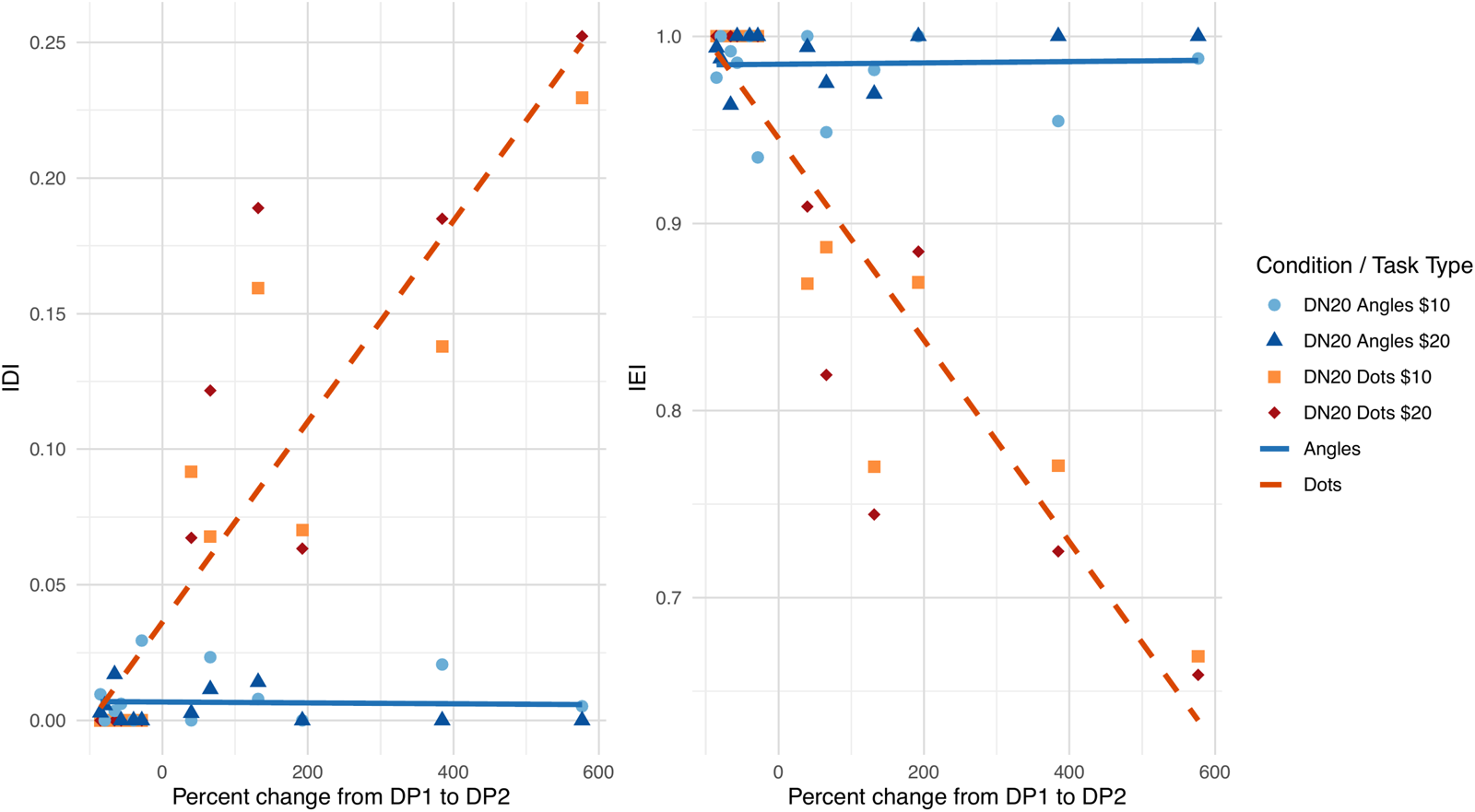
Figure 4 plots the IDI and IEI measures for both tasks in DN20, disaggregated by task type and prize size. This allows us to contrast the two tasks: for the dot-counting task, the best-fit line slopes steeply upward (IDI) and downward (IEI) as incentives increase, while for the angle-judgment task, both lines are nearly flat across the full range of incentive variation. This visual pattern maps directly onto the statistical results in Tables 5 and 6. In the dots task, all six pairwise NIS inequalities in the direction of increasing incentives are violated at conventional significance levels (p  $ \lt $ 0.01 for all comparisons), with the largest relative improvement of 24.0% arising when switching from the lowest to the highest incentive quartile. By contrast, in the angles task, the NIS inequalities are not systematically violated in the direction of increasing incentives, with p-values ranging from 0.08 to 0.80 and the RHS occasionally falling below the LHS, suggesting no meaningful expansion of attentional capacity with higher stakes.
Incentive responsiveness of NIS violations by task type and session prize (DN20)

Figure 4 Long description
The left panel plots IDI and the right panel plots IEI against the percent change in reward from DP1 to DP2. Four marker groups distinguish Angles with a $10 prize, Angles with a $20 prize, Dots with a $10 prize, and Dots with a $20 prize. Light-blue circles and dark-blue triangles represent the Angles conditions; orange squares and red diamonds represent the Dots conditions. Each panel contains two fitted lines, pooling prize sizes within each task: a solid blue line for Angles and a dashed orange line for Dots. As incentives increase, the Dots line rises steeply in the IDI panel and falls steeply in the IEI panel. The Angles lines remain nearly flat, with IDI close to zero and IEI close to one.
NIS inequalities in direction of increasing incentives (aggregate data pooled across prize sizes from the Dot task of DN20)

Table 5 Long description
Columns list DP 1 incentive quartile, DP 2 incentive quartile, LHS, RHS, whether NIS inequality fails, and p-value. For DP 1 in the 1st quartile, LHS is 6.18 and RHS rises from 7.05 for DP 2 in the 2nd quartile, to 8.26 for the 3rd quartile, and 9.30 for the 4th quartile; each row is marked Yes with p-value less than 0.01. For DP 1 in the 2nd quartile, LHS is 20.62 and RHS is 24.16 for DP 2 in the 3rd quartile and 27.20 for the 4th quartile; both are marked Yes with p-value less than 0.01. For DP 1 in the 3rd quartile and DP 2 in the 4th quartile, LHS is 40.05 and RHS is 45.09, marked Yes with p-value less than 0.01.
Aggregate NIS test results of the Angle task of DN20

Table 6 Long description
Pairwise comparisons between DP 1 and DP 2 incentive quartiles are listed with LHS and RHS values, an indicator for NIS inequality fail, and a p-value. For 1st versus 2nd, LHS is 5.84 and RHS is 5.69, NIS inequality fail is No, p-value 0.78. For 1st versus 3rd, LHS is 5.84 and RHS is 5.94, NIS inequality fail is Yes, p-value 0.29. For 1st versus 4th, LHS is 5.84 and RHS is 5.78, NIS inequality fail is No, p-value 0.63. For 2nd versus 3rd, LHS is 16.62 and RHS is 17.37, NIS inequality fail is Yes, p-value 0.08. For 2nd versus 4th, LHS is 16.62 and RHS is 16.89, NIS inequality fail is Yes, p-value 0.32. For 3rd versus 4th, LHS is 28.80 and RHS is 28.00, NIS inequality fail is No, p-value 0.80.
Importantly, these results reflect within-subject incentive variation: subjects were exposed to all incentive levels within their session, so the differences in behavior across quartiles reflect responses to the incentive they faced. This contrast between the two tasks mirrors the difficulty gradient documented in Figure 3 for the CCLN experiment, where harder tasks (Level 1) showed a flatter slope of incentive responsiveness relative to easier tasks (Level 6). The angle-judgment task can be understood as an extreme case of this pattern: a perceptual judgment so resistant to effortful improvement that it behaves as though perceptual capacity is effectively fixed, consistent with the capacity-constrained learning model. Unlike dot-counting (where additional effort translates into measurable accuracy gains) judging angles appears to impose a hard perceptual limit that incentives alone cannot overcome.
Thus, NIS is a useful condition for demarcating the kinds of problems in which the returns to cognitive effort are negligible (relative to the costs). An interesting avenue for future work would be to verify the condition in settings where incentives may not be monotonically increasing.
5. Discussion
Our findings suggest that the failures of NIS observed across multiple datasets are not random but instead track systematic changes in incentives. In DN23, CCLN, and DN20 (dots), violations occur precisely when incentives increase, consistent with the view that higher stakes expand the effective capacity of attention. By contrast, the absence of violations in DN20 (angles) shows that not all perceptual tasks are equally incentive-responsive: some limits appear “hard” and insensitive to payoff variation. This heterogeneity implies that the role of incentives in shaping attention is conditional, operating strongly in domains where effortful attention can augment perception, but weakly where perceptual constraints are rigid. Taken together, these results clarify the contribution of the NIS test: it serves both as a diagnostic for capacity-constrained learning and as a tool for mapping when and how incentives shape the scope of human attention.
One of the key questions raised by the application of NIS in this paper is how to characterize the class of tasks that fall within the capacity-constrained learning paradigm, and those that do not. By using NIS as a diagnostic tool, an experimentalist can assess whether performance in a given task is consistent with a fixed capacity constraint, or instead responds to incentives in a way that suggests an expansion of attention. Doing so requires experimental designs in which the underlying states are well defined and observable to the analyst, the action set and payoff mapping are held fixed across incentive treatments, and incentives vary only in scale. Within-subject designs with randomized exposure to incentive levels are particularly useful, as they allow differences in observed behavior to be interpreted as changes in learning rather than differences in subject composition, and they provide the repeated observations needed to estimate state-dependent choice frequencies with precision.
A closely related direction for future research is to explicitly manipulate the learning feasibility set itself, for example by introducing additional noise, imposing time limits, or varying task difficulty. While the analysis of Caplin et al. (Reference Caplin, Csaba, Leahy and Nov2020) shows that NIS is rejected across all difficulty levels in their task, that design was not intended to test whether increased difficulty shifts tasks into or out of the capacity-constrained regime. Experiments that independently vary incentives and feasibility, while maintaining a fixed mapping between states, actions, and payoffs, would therefore be particularly informative in clarifying which task characteristics are conducive to fixed-capacity behavior and which are not.
Our test may also apply to strategic settings with state-dependent utility, where players face uncertainty about an exogenous state of the world. Previous work applying rational inattention models to games includes de Clippel and Rozen (Reference de Clippel and Rozen2020), Spurlino (Reference Spurlino2022), and Almog and Martin (Reference Almog and Martin2024). In such settings, NIS can be used to test whether players’ perceptual constraints are fixed or respond to incentives. Relatedly, Caplin and Martin (Reference Caplin and Martin2015) establish a connection between rational inattention and quantal response equilibrium (QRE): NIAS is satisfied by the choices that arise from QRE if and only if the noise is small. This suggests that NIS and related conditions can help distinguish models of noisy perception (consistent with Bayesian learning) from models of noisy response (such as standard QRE). However, our framework does not directly apply to games (or individual decision problems) that do not have an exogenous state and prior, such as the complete-information strategic settings studied by Goeree and Holt (Reference Goeree and Holt2001) and the endogenous-state dynamic decision problem studied by Houser et al. (Reference Houser, Keane and McCabe2004). Extending NIS to such environments, where the relevant “state” is endogenous behavior, is a potential direction for future research.
Supplementary material
The supplementary material for this article can be found at https://doi.org/10.1017/eec.2026.10065.
Data availability statement
Data and reproduction materials are available at https://doi.org/10.7910/DVN/IEXCE4. This paper reanalyzes previously published and public data.
Acknowledgements
We thank the Editor, three anonymous referees, Federico Echenique, Mark Dean, and Gerelt Tserenjigmid for helpful comments.
Funding statement
The authors acknowledge support from the Sloan Foundation under the “Cognitive Economics at Work” grant.
Competing interests
The authors declare no competing interests.
Ethical standards
This paper reanalyzes previously published and public data and does not report newly collected human-subjects data.
Use of artificial intelligence
OpenAI Codex was used to assist with review of the manuscript and replication code and to draft accessibility descriptions. The authors reviewed the resulting suggestions and descriptions and take full responsibility for the final content and accuracy of the article and replication materials.






 Open access

