





1. Introduction
Diffusiophoresis (Derjaguin et al. Reference Derjaguin, Dukhin and Korotkova1993) is an electrokinetic mechanism to create a directed transport of a charged colloid mediated by an ionic concentration gradient. The osmotic pressure gradient created by the solute concentration gradient polarizes the electric double layer (EDL) around the charged particle. As a result, the charged particle acquires momentum through the chemiphoresis mechanism. Another part of the diffusiophoresis mechanism, the electrophoresis, arises due to the difference in diffusivity of ionic species. Under a thin Debye layer consideration, Prieve et al. (Reference Prieve, Anderson, Ebel and Lowell1984) determined an expression for the velocity of a rigid charged particle in diffusiophoresis. Since then, various aspects of diffusiophoresis have been investigated through theoretical, numerical and experimental approaches (Ebel et al. Reference Ebel, Anderson and Prieve1988; Velegol et al. Reference Velegol, Garg, Guha, Kar and Kumar2016; Shim Reference Shim2022; Ault & Shin Reference Ault and Shin2025).
The diffusiophoresis of nanodroplets has relevance in several practical contexts such as water purification, soil and the petroleum industry (Yang et al. Reference Yang, Shin and Stone2018; Park et al. Reference Park, Lee, Yoon and Shin2021; Chuang et al. Reference Chuang, Chen, Chang, Chien, Liao and Lee2025). In a biomedical context, droplets serve as carriers for therapeutic agents, imaging probes and biomolecules, and function as models of cells and vesicles (Torchilin Reference Torchilin2005; Pattni et al. Reference Pattni, Chupin and Torchilin2015; Borden et al. Reference Borden, Shakya, Upadhyay and Song2020). Such droplets are also widely used in microfluidics platformed as microreactors and functional carriers for chemical and biological payloads (Li et al. Reference Li, Brinkmann, Pagonabarraga, Seemann and Fleury2018). Directed transport of liquid droplets enables targeted delivery, selective separation and sorting, enhanced mixing and reaction efficiency, and precise manipulation of microscale chemical and biological environments (Duong et al. (Reference Duong, Ganguly, Gupta and Shin2026) and references therein). The stability of dispersed fluid particles, such as nanobubbles and oil droplets, is largely governed by the ionic or non-ionic surfactants.
Diffusiophoresis of non-ionic surfactant-stabilized emulsion droplets under concentration gradients has been studied both theoretically and experimentally by several authors, namely Kagan et al. (Reference Kagan, Laocharoensuk, Zimmerman, Clawson, Balasubramanian, Kang, Bishop, Sattayasamitsathit, Zhang and Wang2010), Izri et al. (Reference Izri, Van Der Linden, Michelin and Dauchot2014), Massarweh & Abushaikha (Reference Massarweh and Abushaikha2020) and Moragues et al. (Reference Moragues, Arguijo, Beneyton, Modavi, Simutis, Abate, Baret, deMello, Densmore and Griffiths2023). The accumulation of surfactants at the droplet surface reduces the surface tension and prevents the coalescence of droplets. However, an inhomogeneous distribution of surfactants due to the adsorption and desorption of surfactants at the interface and surface convection can generate localized Marangoni stress. Surfactants are dissolved in the fluid and a kinetic exchange at the interface occurs for the soluble surfactants. Thus, the dynamics of a surfactant-laden droplet becomes complicated owing to the mutual interactions of diffusiophoresis, Marangoni stress, hydrodynamic stress and the exchange of soluble surfactants between the bulk fluid and the interface. Self-propulsion of active droplets governed by the interaction of Marangoni stress and diffusiophoresis is studied by Morozov & Michelin (Reference Morozov and Michelin2019) and it is shown that by varying the droplet size a transition arises from steady self-propulsion to a steady symmetric extensile flow with no net propulsion of the droplet. The opposite interaction between diffusiophoresis and Marangoni effects on the dynamics of an active droplet is analysed by Wang et al. (Reference Wang, Zheng and Li2024), which shows that the velocity reaches a plateau at a large Péclet number, the parameter which measures the convection to diffusion transport. Recent studies on the dynamics of Marangoni-driven self-propelled active droplets are reviewed by Michelin (Reference Michelin2023). Marangoni stress created by spontaneously solubilizing droplets in a surfactant-saturated outer phase and its impact on self-propulsion of droplets is studied by Kim et al. (Reference Kim, Balaj and Zarzar2024). These studies on analysing the dynamics of surfactant laden droplets have addressed the situation of non-ionic surfactants.
The ionic surfactants create a surface charge density and the droplet therefore experiences Maxwell stress in addition to Marangoni and hydrodynamic stresses. For nanobubbles, the adsorbed charge generates a size-dependent restoring force against thermodynamic perturbations (Zhang et al. Reference Zhang, Guo and Zhang2020). A high
 $\zeta$
-potential typically creates repulsive forces that prevent coalescence, contributing to stabilization (Nirmalkar et al. Reference Nirmalkar, Pacek and Barigou2018). The charging mechanisms of non-polar oil droplets with low dielectric constant are dominated by the specific adsorption of ionic surfactants. Recent experiments (Wang et al. Reference Wang, Shapiro and Andersen2025) demonstrate that oil droplets in aqueous solutions under salinity gradients are stabilized primarily by these surface-active components. This shows that characterization of surfactant adsorption at the interface at both equilibrium and the dynamic state is important in analysing the electrokinetics of fluid droplets in an aqueous medium.
Over the years, several studies on the diffusiophoresis of a charged droplet have been reported in the literature by considering the surfactant-free droplet surface (Yang et al. Reference Yang, Shin and Stone2018; Wu et al. Reference Wu, Jian, Fan, Tseng, Wan and Lee2021b ; Fan et al. Reference Fan, Wu, Jian, Tseng, Wan, Tseng, Lin and Lee2022; Samanta et al. Reference Samanta, Mahapatra, Ohshima and Gopmandal2023). In those studies it is demonstrated that the Maxwell traction created by the macroscopic electric field at the interface plays a major role in determining the diffusiophoretic mobility of the droplet. For a negatively charged droplet in a concentration gradient of an electrolyte with lower cationic diffusivity, the electrophoresis part creates a positive mobility, which may cooperate with the chemiphoresis part. However, for a low viscous droplet the chemiphoresis part may drag the droplet in the direction opposite to the imposed concentration gradient. Such a phenomenon is termed as the double layer polarization of the second kind (DLP-II), in which the strong surface charge repels the coions and prevents the diffusion across the double layer. This leads to a repulsive force on the droplet, creating a force counteracting with the electrophoresis part. In this case the droplet can have a mobility opposite to the direction of the concentration gradient (negative mobility).
When the charging mechanisms of the non-polar droplet are considered to be due to the specific adsorption of ionic surfactant then the phoretic transport, either electrophoresis (governed by an externally imposed electric field) or diffusiophoresis, become different from the case of droplet surface with constant charge density. In such cases, the dynamics becomes complicated owing to the Marangoni stress generated by the non-uniform surfactant distribution on the droplet surface, as well as the kinetic exchange of ionic surfactant at the interface. The non-uniform distribution of ionic surfactant at the interface also creates a non-homogeneous surface charge, which generates a non-homogeneous EDL around the particle. This non-homogeneous EDL augments the double layer polarization (DLP) effect, creating a stronger chemiphoresis. Baygents & Saville (Reference Baygents and Saville1988) have shown that the Marangoni stress due to the formation of the non-uniform ionic surfactant may enhance the positive mobility of the droplet. However, their formulation assumed zero surface diffusivity
 $(D_s=0)$
and instantaneous equilibrium (
 $k_a\to \infty$
,
 $k_d\to \infty$
) between the interface and the immediately adjacent electrolyte. These assumptions correspond to vanishing mobility of interfacial charge and infinitely fast kinetic exchange, which are difficult to justify physically because adsorption and desorption rates are thermodynamically coupled to the equilibrium charge density or
 $\zeta$
-potential. Their model uses a linear (Henry-type) adsorption relation, which is valid only in the dilute limit. Real surfactants exhibit nonlinear adsorption due to finite site availability and lateral interactions, well described by the Langmuir or Frumkin isotherms. The linear assumption neglects saturation effects, leading to an inaccurate prediction of the surface tension gradient, and thus, Marangoni stress and interfacial slip at high surface coverage. Moreover, Baygents & Saville (Reference Baygents and Saville1988) effectively treated ordinary electrolyte ions (e.g. K
 $^{+}$
) as the adsorbing species, overlooking the role of true surface-active ions such as DS
 $^{-}$
(dodecyl sulphate ions) that control interfacial tension and compositional Marangoni stress. Consequently, their theory captures only the electrocapillary limit of electrophoresis but not the finite-rate, surfactant-driven dynamics that govern real fluid interfaces. More recently, Hill (Reference Hill2025) developed a comprehensive framework for the electrophoresis of fluid droplets that includes interfacial kinetic exchange and charge mobility of ionic surfactants. Unlike earlier models such as the uniform-charge formulation of Booth (Reference Booth1951), the mercury-drop model of Ohshima et al. (Reference Ohshima, Healy and White1984) and the equilibrium-interface theory of Baygents & Saville (Reference Baygents and Saville1988), Hill’s analysis incorporates finite adsorption–desorption kinetics (limited to the linear Henry model), lateral charge transport and Marangoni stress within the weak-field approximation. This study demonstrated that finite interfacial mobility of surface charges regularizes the singular electrophoretic mobility reported for highly charged drops and bubbles (Schnitzer et al. Reference Schnitzer, Frankel and Yariv2014; Wu et al. Reference Wu, Fan, Jian and Lee2021a
) and that the adsorption kinetics crucially determine whether an interface behaves as mobile or effectively rigid. Despite these advances, a corresponding theoretical framework for diffusiophoresis that accounts for finite interfacial kinetics and charge mobility remains lacking.
In this study, we investigate the diffusiophoresis of a non-polarizable droplet laden with soluble ionic surfactant. The surface charge of the droplet arises from the adsorption of ionic surfactant molecules at the fluid–fluid interface. The interfacial transport of surfactant is formulated through a mass-balance framework incorporating Langmuir adsorption kinetics, where both adsorption and desorption fluxes are explicitly modelled. The electrokinetics outside the droplet is governed by the standard Poisson–Nernst–Planck–Stokes model, which is coupled with the flow inside the droplet, governed by the Stokes equation, through the interfacial stress balance condition and the kinetic exchange of soluble surfactants. This coupled system is solved through a first-order perturbation approach, limited to a linear order of the externally imposed ionic concentration gradient. Analytical expressions for the diffusiophoretic mobility and interfacial velocity are obtained under the Debye–Hückel (D–H) and thin double-layer approximations in the regime corresponding to negligible desorption. Our results show that the absence of the DLP-II effect, by which the droplet is pushed towards the lower ionic concentration side, as reported in the literature (Wu et al. Reference Wu, Jian, Fan, Tseng, Wan and Lee2021b
; Fan et al. Reference Fan, Wu, Jian, Tseng, Wan, Tseng, Lin and Lee2022; Samanta et al. Reference Samanta, Mahapatra, Ohshima and Gopmandal2023) in the context of diffusiophoresis of droplets with constant immobile surface charge density. Existing studies on droplet electrophoresis by considering a uniformly charged interface (Schnitzer et al. Reference Schnitzer, Frankel and Yariv2014; Wu et al. Reference Wu, Fan, Jian and Lee2021a
) found that the mobility encounters a singularity and the Maxwell stress becomes unbounded when the
 $\zeta$
-potential is increased beyond the D–H limit. We find that the presence of Marangoni stress and mobility of surface ions create a smooth dependence of the diffusiophoretic mobility on the surface charge density. At a higher desorption kinetics of soluble surfactant, the droplet velocity increases significantly along the direction of the imposed concentration gradient and is independent of the diffusion potential. This result highlights the crucial role of surfactant dynamics in controlling droplet transport. Thus, the present study provides insights for the design of responsive microfluidic platforms and controlled emulsion systems, where tuneable interfacial kinetics and mixed electrolytes may be exploited to achieve targeted transport, selective sorting or trapping, and controlled manipulation of droplets under varying chemical conditions.
2. Mathematical formulation
We consider the diffusiophoresis of a non-conducting, immiscible and neutrally buoyant spherical droplet of a viscous dielectric liquid with radius
 $a$
and viscosity
 $\overline {\mu }$
. The droplet is suspended in an electrolyte solution of viscosity
 $\mu$
and permittivity
 $\varepsilon _e$
. The electrolyte consists of a simple supporting salt, e.g. NaCl, KCl or acid HCl and a soluble ionic surfactant, such as sodium dodecyl sulphate (SDS) or sodium dodecylbenzene sulphonate. The surfactant dissociates into an anionic surface-active species and its counterion. We assume that only the anionic species adsorbs on to the droplet surface and exchanges with the adjacent electrolyte. The droplet is translating with the diffusiophoretic velocity
 $\tilde {U}_{D}$
, unknown a priori, in response to an externally imposed ionic concentration gradient
 $\tilde {\boldsymbol{\nabla }}{\tilde {n}^{\infty }}$
. Variables with a tilde are dimensional. The spherical polar coordinate (
 $r,\theta ,\varphi$
) is adopted with its origin fixed at the centre of the droplet and
 $z$
-axis (
 $\theta$
= 0) is along the imposed concentration gradient
 $\tilde {\boldsymbol{\nabla }}{\tilde {n}^{\infty }}$
(figure 1). We assume that the problem is axially symmetric with
 $z$
-axis as the axis of symmetry.
Problem description and spherical polar coordinate system for the diffusiophoresis of a surfactant-laden liquid droplet in an electrolyte solution subjected to an ionic concentration gradient.

The motion of ionized incompressible Newtonian electrolyte outside the droplet can be expressed in the non-dimensional form as
 \begin{align} -\boldsymbol{\nabla }\!p+{\nabla} ^{2}\boldsymbol {u}-(1/2)(\kappa a)^{2} \rho _e \boldsymbol{\nabla }\psi&=0,\end{align}
 \begin{align} \boldsymbol{\nabla }\boldsymbol{\cdot }\boldsymbol {u}&=0,\end{align}
where
 $\boldsymbol {u}=v \boldsymbol{e}_r+ u \boldsymbol{e}_\theta$
is the velocity vector, with
 $v$
and
 $u$
are the radial and polar velocity components, respectively;
 $t$
is the time and
 $p$
is the pressure. The governing equations are non-dimensionalized using the droplet radius
 $a$
as the characteristic length scale, the velocity scale
 $U_{0}=\varepsilon _{e}\psi _{0}^{2}/(a\mu )$
, the time scale
 $\tau =a/U_{0}$
and the pressure scale
 $\varepsilon _{e}\psi _{0}^{2}/a^{2}$
. Here,
 $\mu$
is the viscosity of the electrolyte medium and
 $\psi _{0}=k_{B}T/e$
is the thermal potential. The electric potential
 $\psi$
is scaled by
 $\psi _{0}$
. The space charge density
 $\rho _e$
, defined as
 $\rho _e=\textstyle \sum _{i}{z_{i}n_{i}}$
, is scaled by
 $eI^{\infty }$
, where
 $e$
is the elementary charge and
 $I^{\infty }$
is the bulk ionic strength governed by
 $I^{\infty }=(1/2)\sum _{i=1}^{N}{z^{2}_{i}\tilde {n}^{\infty }_{i}}$
. Here,
 $\tilde {n}_{i}^{\infty }$
denotes the dimensional bulk concentration (number density) of the
 $i$
th ionic species in absence of the imposed electrolyte concentration gradient. The values of
 $\tilde {n}_{i}^{\infty }$
are determined from the total bulk concentration of the electrolyte
 $\tilde {n}^{\infty }$
. For example, for a binary electrolyte of
 $z_1:z_2$
type,
 $\tilde {n}_{1}^{\infty }=-z_{2}\tilde {n}^{\infty }$
and
 $\tilde {n}_{2}^{\infty }=z_{1}\tilde {n}^{\infty }$
. We denote
 $n_{i}$
as the dimensionless ionic concentration (number density) of the ith ionic species, scaled by
 $I^{\infty }$
. Here,
 $\kappa ^{-1}$
is the Debye length defined as
 $\kappa ^{-1}=\sqrt {\epsilon _e\psi _{0}/2I^{\infty }e}$
. Further, the non-dimensional equation for the flow inside the droplet is
 \begin{align} \mu _{r} {\nabla} ^{2}\overline {\boldsymbol {u}}-\boldsymbol{\nabla }\overline {p}=0, \\[-28pt] \nonumber \end{align}
 \begin{align} \boldsymbol{\nabla }\boldsymbol{\cdot }\overline {\boldsymbol {u}}=0, \\[0pt] \nonumber \end{align}
where
 $\overline {\boldsymbol {u}}=\overline {v} \boldsymbol{e}_r +\overline { u} \boldsymbol{e}_\theta$
is the velocity vector and
 $\overline {p}$
is the pressure inside the droplet. Here
 $\mu _{r}\,(=\overline {\mu }/\mu )$
is the viscosity ratio between the viscosity of the drop and the viscosity of the ionized fluid. The overbar indicates it is defined inside the droplet. The droplet is assumed to contain no free ions and thus, the electric body-force term does not appear in (2.2a
). In (2.1a
) and (2.2a
), the inertial terms are neglected since the Reynolds numbers
 $\textit{Re}$
and
 $\overline {\textit{Re}}$
are
 $O(10^{-4})$
and therefore inertia has no influence on the fluid motion or on the droplet dynamics. The boundary conditions for the velocity field at the droplet surface (
 $r=1$
) are the tangential velocity continuity and fluid impermeability conditions, i.e.
 \begin{equation} \boldsymbol {u}=\overline {\boldsymbol {u}},\,\,\,\,\,\boldsymbol {u}\boldsymbol{\cdot }\boldsymbol {n}=0. \end{equation}
Here,
 $\boldsymbol {n}$
is the outward unit normal vector at the surface. Since the interfacial stress balance plays a central role in droplet diffusiophoresis, its accurate derivation is essential in the presence of ionic surfactants at the interface. The tangential stress balance condition is given by (Slattery et al. Reference Slattery, Sagis and Oh2007; Manikantan & Squires Reference Manikantan and Squires2020)
 \begin{equation} \boldsymbol {n}\boldsymbol{\cdot }(S_{H}-\overline {S}_{H})\boldsymbol{\cdot }\boldsymbol {t}=-\textit{Ma}\boldsymbol{\nabla} _{s}\gamma \boldsymbol{\cdot }\boldsymbol {t}. \end{equation}
Here,
 $S_{H}$
denotes the hydrodynamic stress tensor, defined as
 $S_{H}=-p\boldsymbol{I}+[\boldsymbol{\nabla }\boldsymbol {u} + (\boldsymbol{\nabla }\boldsymbol {u})^T]$
, scaled by
 $\mu U_{0}/a$
and
 $\boldsymbol{t}$
is the unit tangential vector at the interface. The variable
 $\gamma$
represents the dimensionless surface tension and
 $\boldsymbol{\nabla} _{s}=(\boldsymbol{I}-\boldsymbol {n}\boldsymbol {n})\boldsymbol{\cdot }\boldsymbol{\nabla}$
is the gradient operator along the surface. The surface tension is scaled with
 $\varGamma ^{\infty } k_{B}T$
, where
 $\varGamma ^{\infty }$
is the maximum surface packing concentration of the surfactant. Here
 $\textit{Ma}$
is the Marangoni number defined as
 $\textit{Ma}=ea\varGamma ^{\infty }/\epsilon _e\psi _{0}$
or equivalently,
 $\textit{Ma}=k_{B}T\varGamma ^{\infty }/{\mu U_{0}}$
, which measures the ratio between the characteristic surface-pressure stress generated by surfactant accumulation, to the viscous stress scale. In the present study, the deformation of the droplet is not considered as it has negligible impact on the droplet dynamics. This assumption is justified by the fact that the capillary number remains very small as the applied concentration gradient
 $\alpha \sim O(10^{-3})$
, as discussed later. The surface tension and surfactant concentration are related through the Gibbs adsorption isotherm (Kralchevsky & Danov Reference Kralchevsky and Danov2015; Manikantan & Squires Reference Manikantan and Squires2020),
 \begin{equation} -\boldsymbol{\nabla} _{s}\gamma =\boldsymbol{\nabla} _{s}\varPi =\sum _{i}{\varGamma _{i}\boldsymbol{\nabla} _{s}\mu _{s,i}}, \end{equation}
where
 $\varPi$
is the surface pressure arising from the adsorption of surfactant component
 $i$
at the interface with interfacial concentration
 $\varGamma _{i}$
. The variable
 $\mu _{s,i}$
denotes the interfacial electrochemical potential of the surfactant species
 $i$
. In the present study, we restrict to a single surfactant species, characterized by the surface concentration
 $\varGamma$
, electrochemical potential
 $\mu _{s}$
and valency
 $z_{s}$
. Here the interfacial surfactant concentration
 $\tilde {\varGamma }$
is scaled by
 $\varGamma ^{\infty }$
. The interfacial electrochemical potential of the surfactant can be obtained as (Prosser & Franses Reference Prosser and Franses2001)
 \begin{equation} \mu _{s}=\mu _{s0}+\ln [\varGamma /(1-\varGamma )]+z_{s}\psi _{s}. \end{equation}
Here,
 $\mu _{s0}$
is the reference chemical potential. The second term on the right-hand side represents the non-electrostatic contribution arising from surfactant adsorption at the interface, modelled here using the Langmuir isotherm. The surface gradient of this contribution gives rise to the Marangoni stress. The last term corresponds to the electrostatic contribution of the adsorbed charged surfactant, where
 $\psi _s=\psi (r=1,\theta )$
is the electrostatic potential evaluated at the droplet interface. Substituting the stresses in the (2.4) and performing algebraic simplification, we get
 \begin{equation} \left (\partial _{r}u-u/r\right )|_{r=1^+}-\mu _r \left (\partial _{r} \overline {u}-\overline {u}/r\right )|_{r=1^-} ={\left [\sigma \partial _{\theta } \psi \right ]}_{r=1}+\textit{Ma}(1-\varGamma )^{-1}\partial _{\theta } \varGamma . \end{equation}
The adsorbed surfactant creates the dimensionless surface charge density
 $\sigma =z_{s}\textit{Ma}\varGamma$
which creates the Maxwell stress. The Marangoni stress arise due to the nonuniformity of
 $\varGamma$
at the interface. In (2.7), the left-hand side provides the difference in the hydrodynamic shear stresses at the interface. The first term of right-hand side presents the tangential Maxwell stress created by the charged surfactant and the second term corresponds to the Marangoni stress. An interplay between these stresses governs the droplet motion. The normal stress balance condition at the surface is not required, as the droplet is considered undeformed. Instead, the impermeability condition given by (2.3) is employed as the second boundary condition for fluid flow outside the droplet.
The surfactant concentration at the interface is governed by the mass-balance principle as
 \begin{equation} \boldsymbol{\nabla} _{s}\boldsymbol{\cdot }\left [\textit{Pe}_{s}\varGamma \boldsymbol{u}_{s}-\boldsymbol{\nabla} _{s}\varGamma /(1-\varGamma )-z_{s}\varGamma \boldsymbol{\nabla} _{s}\psi _{s}\right ]=C_{a}{n_{N,s}}(1-\varGamma )-C_{d}\varGamma . \end{equation}
The right-hand side accounts for the interfacial mass exchange arising from adsorption–desorption kinetics, i.e.
 $J_{\boldsymbol {n}}=C_{a}{n_{N,s}}(1-\varGamma )-C_{d}\varGamma$
. The coefficients
 $C_{a}$
and
 $C_{d}$
are defined as
 $C_{a}=k_{a}I^{\infty }a^{2}/D_{s}$
and
 $C_{d}=k_{d}a^{2}/D_{s}$
, where
 $k_{a}$
and
 $k_{d}$
are, respectively, the adsorption and desorption rate constant of soluble surfactant. Here,
 $\varGamma =\tilde {\varGamma }/\varGamma ^\infty$
and
 $\textit{Pe}_s=U_0 a/D_s$
is the surface Péclet number, which measures the importance of advection relative to diffusion of the adsorbed surfactant at the interface. Here,
 $n_{N}$
denotes the concentration of the surface-active anionic surfactant species in the surrounding electrolytes, and
 $n_{N,s}\,(=n_N|_{r=1})$
represents its value evaluated at the interface. The quantity
 $n_{N,s}$
is distinct from the surface concentration of specifically adsorbed surfactant molecules,
 $\varGamma$
. The two are interfacial variables of different dimensionality and are coupled through adsorption kinetics (2.8). In the limiting case where the droplet is coated with insoluble, compressible ionic surfactant, that is, when the surfactants are irreversibly adsorbed at the interface (
 $k_{d}=0$
) and do not exchange with the surrounding electrolytic medium during diffusiophoresis, the governing equation for the interfacial surfactant concentration simplifies to
 \begin{equation} \boldsymbol{\nabla} _{s}\boldsymbol{\cdot }\left [\textit{Pe}_{s}\varGamma \boldsymbol{u}_{s}-\boldsymbol{\nabla} _{s}\varGamma /(1-\varGamma )-z_{s}\varGamma \boldsymbol{\nabla} _{s}\psi _{s}\right ]=0. \end{equation}
The governing equations for the concentration of the
 $i$
th ionic species
 $n_{i}$
, derived from the conservation of ionic flux, is given by
 \begin{equation} \boldsymbol{\nabla }\boldsymbol{\cdot }[\textit{Pe}_{i}n_{i}\boldsymbol {u}-n_{i}\boldsymbol{\nabla }\mu _{i}]=0, \end{equation}
in which
 $\mu _{i}$
denotes the dimensionless electrochemical potential, defined as
 $\mu _{i}=\mu _{i0}+z_{i}\psi +\ln {n_{i}}$
. Here,
 $\textit{Pe}_i=\varepsilon _e \psi _0^{2}/\mu D_i$
is the Péclet number of the
 $i$
th ionic species, characterizing the ratio of advective to diffusive transport of ions in which
 $D_i$
is the diffusion coefficient of the
 $i$
th ionic species. In contrast to the surface Péclet number
 $\textit{Pe}_{s}$
, the bulk Péclet number
 $\textit{Pe}_i$
relates convective to diffusive transport of the
 $i$
th ionic species in the surrounding electrolyte. The boundary conditions at the interface for the ionic species are
 \begin{equation} \bigl (\textit{Pe}_{i}n_{i}\boldsymbol{u}-n_{i}\boldsymbol{\nabla }\mu _{i}\bigr )\boldsymbol{\cdot }\boldsymbol{n} = \delta _{iN}\,\bigl (I_{d}\varGamma - I_{a}n_{N,s}(1-\varGamma )\bigr ),\,\,\,i=1,\ldots ,N, \end{equation}
where
 $ \delta _{iN}$
is the Kronecker delta and
 $i=N$
refers to the anionic surfactant species that adsorbs at the droplet interface and undergoes adsorption–desorption exchange with the adjacent electrolytes. Here, the coefficients
 $I_{a}$
and
 $I_{d}$
, which arise due to the kinetic exchange between the interface and the adjacent electrolytes, are defined as
 $I_{a}=k_{a}\varGamma ^{\infty }a/D_{N}$
and
 $I_{d}=k_{d}\varGamma ^{\infty }a/(D_{N}I^{\infty })$
.
The governing equation for the electric potential (
 $\psi$
) is the Poisson equation described as
 \begin{equation} {\nabla} ^{2}\psi =-(1/2)(\kappa a)^{2}\textstyle \sum _{i}{z_{i}n_{i}}, \end{equation}
derived from Gauss’s Law. The boundary condition at the surface for electric potential is
 \begin{equation} \boldsymbol {n}\boldsymbol{\cdot }\boldsymbol{\nabla }\psi =-\sigma , \end{equation}
appropriate when the electric permittivity is much larger in the electrolytes than in the droplet.
An externally imposed ionic concentration gradient
 $|\tilde {\boldsymbol{\nabla }} \tilde {n}^{\infty }|\boldsymbol{e}_z$
is imposed in the far field
 $r \to \infty$
. Accordingly, the boundary conditions for ionic concentration
 $n_{i}$
and electric potential
 $\psi$
are obtained as
 \begin{equation} n_i=n^{\infty }_{i}(1+\alpha r\cos \theta )\quad\text{and}\quad\psi =-\alpha \beta r\cos \theta \quad \text{as}\quad r\to \infty , \end{equation}
where
 $n^{\infty }_{i}={\tilde {n}^{\infty }_{i}}/I^{\infty }$
. The parameter
 $\alpha ={|\tilde {\boldsymbol{\nabla }}{\tilde {n}^{\infty }}|a}/{\tilde {n}^{\infty }}$
is the scaled externally imposed ionic concentration gradient, where
 $\tilde {n}^{\infty }$
is the total dimensional bulk electrolyte concentration in absence of the imposed ionic concentration gradient. The concentration gradient is created by setting the far-field concentration of the ith ionic species as
 ${n^{\infty }_{i}}(1+\alpha r\cos \theta )$
, where
 $n^{\infty }_{i}$
is the corresponding equilibrium bulk concentration for
 $\alpha =0$
. Due to the zero net-current condition under no externally imposed electric field, an induced electric field, the diffusion field, develops when the diffusivities of the ionic species are unequal, i.e.
 $\beta ={\sum _{i}{z_{i}D_{i}\tilde {n}^{\infty }_{i}}}/{\sum _{i}{z^{2}_{i}D_{i}\tilde {n}^{\infty }_{i}}}$
is non-zero and the scaled electric potential is
 $-\alpha \beta r\cos \theta$
.
The problem is formulated in a reference frame fixed at the droplet centre, which translates at the diffusiophoretic velocity
 $U_D$
. Under this stationary frame of reference, the fluid far from the droplet is moving with a uniform velocity
 $-U_D \boldsymbol{e}_z$
. Thus, the boundary condition for the fluid flow far from the droplet
 $(r \to \infty )$
is
 \begin{equation} \boldsymbol {u}=-\mu _{D}\alpha \boldsymbol{e}_z. \end{equation}
The diffusiophoretic mobility, denoted by
 $\mu _{D}$
, quantifies the velocity of the droplet per unit concentration gradient (Ganguly et al. Reference Ganguly, Roychowdhury and Gupta2024) and is defined as
 $\mu _{D}=U_{D}/{\alpha }$
. Here,
 $U_{D}$
is the dimensionless diffusiophoretic velocity, scaled by a characteristic velocity scale
 $U_{0}$
, which is not known a priori. Under the steady-state condition,
 $U_{D}$
is determined by imposing the force-free condition, requiring that the net hydrodynamic and electrical forces on an arbitrary control volume enclosing the droplet vanish.
In the context of self-propelling active droplets of size
 $O(10$
–
 $100\,{\unicode{x03BC}} \text{m})$
governed by combined diffusiophoresis and Marangoni effect created by the non-ionic surfactant, several authors (Izri et al. Reference Izri, Van Der Linden, Michelin and Dauchot2014; Schmitt & Stark Reference Schmitt and Stark2016; Michelin Reference Michelin2023; Maass et al. Reference Maass, Michelin and Zarzar2024) have demonstrated a transition from steady propulsion to unsteady or chaotic dynamics as the Péclet number based on the solute diffusivity is increased by increasing the droplet size. In contrast, in the present study, the characteristic droplet size is in the nanoscale (
 $a \sim 50$
nm), and the bulk Péclet number based on the diffusiophoretic velocity of the droplet and droplet size remain lower than 0.04. For a non-ionic surfactant in a diffusion dominated process, a solute concentration gradient develops over a time scale of
 $a^{2}/D_{i}$
. Thus, a steady-state is achieved instantly for the length scale
 $a\sim 50 \,\textrm {nm}$
. In the present formulation the Marangoni stress develops through the non-uniform interfacial distribution of soluble surfactant governed by the advection, diffusion and electromigration along the interface and the kinetic exchange through adsorption–desorption with the suspension medium. Owing to the small length scale and diffusion-dominated transport of surfactant, the transient or unsteady effects decay rapidly, thereby justifying the use of a steady-state approximation. Under such steady-state condition the droplet velocity
 $U_{D}$
can be determined through the balance of the forces acting on the droplet as discussed earlier in this section.
3. Perturbation analysis
If the imposed ionic concentrations at the two ends of the domain of length
 $2\tilde {R}$
are denoted by
 $\tilde {n}^{\infty ,L}$
and
 $\tilde {n}^{\infty ,R}$
, then the associated scaled concentration gradient is obtained by the parameter as
 $\alpha =(\tilde {n}^{\infty ,R}-\tilde {n}^{\infty ,L})a/(0.5(\tilde {n}^{\infty ,R}+\tilde {n}^{\infty ,L})2\tilde {R})\lt a/\tilde {R}$
, as
 $|\tilde {\boldsymbol{\nabla }}{\tilde {n}^{\infty }}|=(\tilde {n}^{\infty ,R}-\tilde {n}^{\infty ,L})/2\tilde {R}$
and
 $\tilde {n}^{\infty }=0.5(\tilde {n}^{\infty ,R}+\tilde {n}^{\infty ,L})$
. Here,
 $\tilde {R}$
is the radius of the computational domain, which must be chosen sufficiently large compared with the droplet radius
 $a$
(i.e.
 $a/\tilde {R} \ll 1$
) for any arbitrary values of
 $\kappa a$
. Consequently, we have
 $\alpha \lt a/\tilde {R}\ll 1$
. This range of
 $\alpha$
is consistent with several experimental studies on diffusiophoresis, where the imposed dimensionless concentration gradient of electrolytes is typically varied in the range
 $\alpha =0.001\,\text{to}\,0.0065$
(Ebel et al. Reference Ebel, Anderson and Prieve1988; Shin et al. Reference Shin, Um, Sabass, Ault, Rahimi, Warren and Stone2016). Under such a small
 $\alpha$
, the variables can be expressed as a linear perturbation from its equilibrium, i.e.
 $\psi =\psi ^{0}(r)+\delta \psi (r,\theta )$
,
 $n_{i}=n^{0}_{i}(r)+\delta n_{i}(r,\theta )$
,
 $\mu _{i}=\mu ^{0}_{i}+\delta \mu _{i}(r,\theta )$
and
 $\boldsymbol{u}=0+\delta \boldsymbol{u}$
, where the quantities with the superscript
 $0$
refer to those at equilibrium, i.e. at
 $\alpha =0$
and the perturbed variables with prefix
 $\delta$
are of
 $O(\alpha )$
. At the equilibrium
 $O(\alpha ^{0})$
, the particle as well as the background ionized fluid is at rest, i.e.
 $\boldsymbol{u}^{0}=0$
. The interfacial surfactant concentration
 $\varGamma$
can be expressed as
 $\varGamma =\varGamma ^{0}+\delta \varGamma$
and consequently, the surface charge density is given by
 $\sigma =\sigma ^{0}+\delta \sigma =\sigma ^{0}+z_{s}Ma\delta \varGamma$
, where
 $z_{s}$
is the valence of the ionic surfactant species and
 $\textit{Ma}$
is the Marangoni number based on
 $\varGamma ^{\infty}$
. In the following subsection, we derive the governing equations for both the equilibrium state and the perturbed regime.
3.1. Equilibrium state
The equilibrium state refers to the situation before applying any external ionic concentration gradient, i.e.
 $\alpha =0$
. At this situation, the ion velocities as well the fluid velocity vanish, which implies that the electrochemical potential gradient must be zero. This gives
 \begin{equation} z_{i}n^{0}_{i}(r)\psi ^{0}_{r}(r)+n^{0}_{i,r}(r)=0. \end{equation}
Here and throughout the paper, the subscripts
 $r$
and
 $rr$
denote the first and second derivatives with respect to the radial coordinate
 $r$
, respectively. Upon integration to the far field, (3.1) gives
 \begin{equation} n^{0}_{i}(r)=n^{\infty }_{i}\exp \big [-z_{i}\psi ^{0}(r)\big ]. \end{equation}
Equation (3.2) is obtained with the condition that the equilibrium potential vanishes at the far field. Applying (3.2) into the Poisson equation (2.12), the equilibrium potential outside the droplet is governed by
 \begin{equation} \psi ^{0}_{rr}(r) + (2/r)\psi ^{0}_{r}(r)= -(1/2)(\kappa a)^2 \textstyle \sum _{i} z_{i} n^{0}_{i}(r) \end{equation}
with the boundary conditions
 \begin{equation} \psi ^{0}_{r}(1)=-z_{s} \textit{Ma}\varGamma ^{0}, \quad \psi ^{0}(r\to \infty )\to 0. \end{equation}
Note that at equilibrium the adsorption and desorption rates are equal, yielding
 $C_{a}n^{0}_{N,s}(1-\varGamma ^{0})=C_{d}\varGamma ^{0}$
. Here,
 $n^{0}_{N,s}$
can be found from (3.2) as
 $n^{0}_{N,s}=(\tilde {n}^{\infty }_{N}/I^{\infty })e^{-z_{N}\zeta }$
, in which
 $\zeta =\psi ^{0}_{s}=\psi ^{0}(r=1)$
is the equilibrium interfacial potential. Thus, the adsorption rate coefficient
 $k_{a}$
can be determined for a prescribed desorption rate coefficient
 $k_{d}$
as
 \begin{equation} k_{a}=(k_{d}/\tilde {n}^{\infty }_{N})\varGamma ^{0}/ \big[(1-\varGamma ^{0})e^{-z_{N}\zeta }\big]. \end{equation}
This relation shows that
 $k_{a}$
(or
 $k_{d}$
) varies with dimensional bulk surfactant concentration (
 $\tilde {n}^{\infty }_{N}$
) and the interfacial electrostatic potential (
 $\zeta$
). Variation in ionic strength influences the
 $\zeta$
-potential. Consequently, the adsorption rate has a dependency on the bulk ionic concentration. For ionic surfactants such as SDS, electrolyte concentration can also influence adsorption energetics and interfacial structure more broadly. In a NaCl–SDS system, NaCl screens electrostatic repulsion between charged surfactant headgroups, promoting closer packing, increased adsorption at interfaces, and a reduction in surface tension (Qazi et al. Reference Qazi, Liefferink, Schlegel, Backus, Bonn and Shahidzadeh2017). Capturing such effects would require a more detailed physicochemical description of the adsorption process, which is beyond the scope of the present study.
3.2. Linear-order analysis
Upon substituting the linear perturbations described above into the governing equations presented in § 2 and separating the perturbed components, we obtain the following set of equations governing the perturbations:
 \begin{align} {\nabla} ^{2}\delta \psi (r,\theta ) &= -(1/2)(\kappa a)^2\textstyle \sum _{i}z_{i}\delta {n_{i}}(r,\theta ),\nonumber\\[-10pt]\end{align}
 \begin{align} n^{0}_{i}(r){\nabla} ^{2}\delta \mu _{i}(r,\theta ) +\boldsymbol{\nabla }n^{0}_{i}(r)\boldsymbol{\cdot }\boldsymbol{\nabla }\delta \mu _{i}(r,\theta )&= \textit{Pe}_{i}\delta \boldsymbol {u}(r,\theta )\boldsymbol{\cdot }\boldsymbol{\nabla }n^{0}_{i}(r),\nonumber\\[-10pt] \end{align}
 \begin{align} \boldsymbol{\nabla }\times \left [\boldsymbol{\nabla }\times \boldsymbol{\nabla }\times \delta \overline {\boldsymbol {u}}(r,\theta )\right ]&=0,\nonumber\\[-10pt]\end{align}
 \begin{align} \boldsymbol{\nabla }\times \{\boldsymbol{\nabla }\times \boldsymbol{\nabla }\times \delta \boldsymbol {u}(r,\theta )\}&=(1/2)(\kappa a)^2 \textstyle \sum _{i}{\boldsymbol{\nabla }\delta \mu _{i}(r,\theta )\times \boldsymbol{\nabla }n^{0}_{i}(r)}.\end{align}
Exploiting the axial symmetry imposed by the externally applied concentration gradient, the first-order perturbation variables can be expressed as separable functions of the radial coordinate multiplied by prescribed angular variations (Ohshima et al. Reference Ohshima, Healy and White1983; Prieve & Roman Reference Prieve and Roman1987). Accordingly, we write
 \begin{align} \delta \psi (r,\theta )&=-\varPsi (r)\alpha \cos \theta ,\nonumber\\[-10pt]\end{align}
 \begin{align} \delta \mu _{i}(r,\theta )&=-z_{i}\varPhi _{i}(r)\alpha \cos \theta ,\nonumber\\[-10pt]\end{align}
 \begin{align} \delta \overline {\boldsymbol {u}}(r,\theta )&=\left [-(2/r)\overline {h}(r)\alpha \cos \theta \right ] \boldsymbol{e}_r+\left [(\overline {h}_{r}(r)+(\overline {h}(r)/r))\alpha \sin \theta \right ]\boldsymbol{e}_\theta ,\nonumber\\[-10pt]\end{align}
 \begin{align} \delta \boldsymbol {u}(r,\theta )&=\left [-(2/r)h(r)\alpha \cos \theta \right ]\boldsymbol{e}_r+\left [(h_{r}(r)+(h(r)/r))\alpha \sin \theta \right ]\boldsymbol{e}_\theta.\end{align}
The corresponding perturbation of the interfacial surfactant concentration is written as (Baygents & Saville Reference Baygents and Saville1988; Hill Reference Hill2025)
 \begin{equation} \delta \varGamma (\theta )=\varDelta _s\alpha \cos \theta . \end{equation}
Substituting (3.7a
) in (3.6a
), the
 $O(\alpha )$
equation of perturbed electric potential outside the droplet is obtained as
 \begin{equation} \mathcal{L}\varPsi (r)=(1/2)(\kappa a)^2\textstyle \sum _{i}z^{2}_{i}n^{0}_{i}\left [\varPsi (r)-\varPhi _{i}(r)\right ]. \end{equation}
The operator
 $\mathcal{L}$
is defined as
 $\mathcal{L}=\partial _{rr}+(2/r)\partial _{r}-2/r^{2}$
, where the subscript indicates a derivative with respect to the radial coordinate. Note that
 $\delta n_{i}(r,\theta )$
present on the right-hand side of (3.6a
) is obtained using (3.7a
) and (3.7b
) in the form
 $\delta n_{i}(r,\theta )=n^{0}_{i}(r)[\delta \mu _{i}(r,\theta )-z_{i}\delta \psi (r,\theta )]$
. The boundary conditions corresponding to the second-order ordinary differential equation (ODE) (3.9) are
 \begin{equation} \varPsi _{r}|_{r=1}=z_{s} \textit{Ma} \Delta _{s}, \quad \varPsi (r)=\beta r \quad \text{as} \quad r \to \infty . \end{equation}
Applying the linear perturbation approximation on the (2.8), we get
 \begin{equation} \begin{aligned} & \textit{Pe}_{s}\varGamma ^{0}\boldsymbol{\nabla} _{s}\boldsymbol{\cdot }\delta \boldsymbol{u}_{s}-({1-\varGamma ^{0}})^{-1}{\nabla} ^{2}_{s}\delta \varGamma -z_{s}\varGamma ^{0}{\nabla} ^{2}_{s}\delta \psi _{s}\\[3pt] & =C_{a}(1-\varGamma ^{0})\delta n_{N,s}-(C_{a}n^{0}_{N,s}+C_{d})\delta \varGamma , \end{aligned} \end{equation}
which further can be written as
 \begin{equation} \begin{aligned} &\textit{Pe}_{s}\varGamma ^{0}(1/\sin \theta )\partial _{\theta }[\sin \theta \delta {u}_{s}]-({1-\varGamma ^{0}})^{-1}(1/\sin \theta )\partial _{\theta }[\sin \theta \partial _{\theta }\delta \varGamma ]\\[3pt] & -z_{s}\varGamma ^{0}(1/\sin \theta )\partial _{\theta }[\sin \theta \partial _{\theta }\delta \psi _{s}]=C_{a}(1-\varGamma ^{0})\delta n_{N,s}-(C_{a}n^{0}_{N,s}+C_{d})\delta \varGamma , \end{aligned} \end{equation}
where
 $\delta u_{s} (=u_{s})$
is the tangential interfacial velocity. Substituting the expression for
 $\delta u_{s}$
and
 $\delta \psi _{s}$
from (3.7) and
 $\delta \varGamma$
from (3.8) and performing algebraic simplification,
 $\varDelta _{s}$
can be obtained as
 \begin{equation} \varDelta _{s}=2\varGamma _{C}\varGamma ^{0}\big [z_{s}\varPsi (1)-\textit{Pe}_{s}h_{r}\big |_ {r=1}\big]+\varGamma _{C}C_{a}(1-\varGamma ^{0})z_{N}n^{0}_{N,s}\big [\varPsi (1)-\varPhi _{N}(1)\big ], \end{equation}
where
 $\varGamma _{C}$
is defined as
 $\varGamma _{C}=(1-\varGamma ^{0})/[2+(C_{a}n^{0}_{N,s}+C_{d})(1-\varGamma ^{0})]$
. Consequently, the surfactant concentration at the interface of the droplet can be expressed as
 \begin{equation} \begin{aligned} \varGamma =&\varGamma ^{0}+\big \{2\varGamma _{C}\varGamma ^{0}\left [z_{s}\varPsi (1)-\textit{Pe}_{s}h_{r}\big |_ {r=1}\right ]+\\[3pt] & \varGamma _{C}C_{a}(1-\varGamma ^{0})z_{N}n^{0}_{N,s}\left [\varPsi (1)-\varPhi _{N}(1)\right ]\big \}\alpha \cos \theta . \end{aligned} \end{equation}
Here,
 $\varGamma ^{0}$
denotes the equilibrium surfactant concentration in absence of the externally imposed concentration gradient, while the second term represents a linear-order perturbation from equilibrium, arising due to the imposed concentration gradient. Equation (3.14) shows that the surfactant distribution is dipolar in nature, varying as
 $\cos \theta$
, with accumulation on one side of the droplet and depletion on the opposite side. This asymmetry results from the combined effects of interfacial advection, surface diffusion, electromigration and adsorption–desorption kinetics under the external field gradient, which together balance each other so that the surfactant distribution becomes steady in the frame moving with the droplet. This asymmetric redistribution leads to a non-uniform surface charge density, surface tension and consequently generates Maxwell and Marangoni stresses along the interface, which contribute to the droplet mobility. In absence of the external gradient, the distribution reduces to the equilibrium uniform state
 $\varGamma =\varGamma ^{0}$
.
Upon inserting the perturbation expansions (3.7) into the linearized Nernst–Planck equation (3.6b
), which governs the
 $O(\alpha )$
response, one obtains the second-order boundary-value problem as
 \begin{equation} \mathcal{L}\varPhi _{i}+(n^{0}_{i,r}/n^{0}_{i})\varPhi _{i,r}=(2\textit{Pe}_{i}/z_{i})(n^{0}_{i,r}/n^{0}_{i})(h/r) \end{equation}
which corresponds to the boundary conditions
 \begin{align} \varPhi _{i,r}|_{r=1} &= \delta _{iN}\big [\big(I_{d}+I_{a}n^{0}_{N,s}\big)\nonumber\\[-1pt] &\quad \big(z_{N}n^{0}_{N,s}\big)^{-1}\,\varDelta _{s} - I_{a}\big(1-\varGamma ^{0}\big)(\varPsi (1)-\varPhi _{N}(1)) \big],\nonumber\\[-10pt]\end{align}
 \begin{align} \varPhi _{i}(r \to \infty ) &= \big [-(1/z_{i})+\beta \big ] r.\nonumber\\[-10pt]\end{align}
Substituting (3.7) into (3.6c ) and (3.6d ) we get
 \begin{align} \mathcal{L}(\mathcal{L}\overline {h})&=0,\end{align}
 \begin{align} \mathcal{L}(\mathcal{L}h)&=(1/2r)(\kappa a)^2\textstyle \sum _{i}z_{i}n^{0}_{i,r}\varPhi _{i} \end{align}
subject to the boundary conditions
 \begin{gather} \overline {h}(1^{-})=0, \quad \overline {h}_{r}(1^{-})=h_{r}(1^{+}), \end{gather}
 \begin{gather} h(1^{+})=0, \quad h_{rr}(r=1^{+})-\mu _{r}\overline {h}_{rr}(r=1^{-})=z_{s}\textit{Ma}\varGamma ^{0} \varPsi (1)-\textit{Ma}(1-\varGamma ^{0})^{-1}\varDelta _{s}, \end{gather}
 \begin{gather} h(r)\to (\mu _{D}/2)r+O(r^{-1}) \quad \text{as} \quad r \to \infty . \end{gather}
The solution of (3.17a ) satisfying (3.18a ) can be obtained as (Ohshima et al. Reference Ohshima, Healy and White1984)
 \begin{equation} \overline {h}(r)=-(1/2)h_{r}(1^{+})[r-r^3]. \end{equation}
Using (3.13) and (3.19) we can construct the second boundary condition of (3.18b ) as
 \begin{equation} h_{rr}(r=1^{+})-3\mu _{r}h_{r}(r=1^{+})=z_{s} \textit{Ma}\varGamma ^{0} \varPsi (1)-\textit{Ma}(1-\varGamma ^{0})^{-1}\varDelta _{s}. \end{equation}
A formal decomposition of the interfacial stress balance (3.20) shows that, in the insoluble-surfactant limit, the Marangoni contribution can offset the Maxwell traction in the tangential stress balance. However, for an ionic surfactant, these two effects are not independent, since the same surfactant redistribution simultaneously modifies both the surface tension and the surface charge density. We reduce the fourth-order ODE (3.17b ) into two coupled second-order ODEs as
 \begin{align} \mathcal{L}(h)&=h_{1},\end{align}
 \begin{align} \mathcal{L}(h_{1})&=(1/2r)(\kappa a)^2\textstyle \sum _{i}z_{i}n^{0}_{i,r}\varPhi _{i},\end{align}
and the corresponding boundary conditions become
 \begin{align} h(1)=0, \quad h_{rr}({r \to \infty })=0, \\[-32pt] \nonumber \end{align}
 \begin{align} h_{1}(1)=(3\mu _{r}+2)h_{r}(r=1^{+})+z_{s}\textit{Ma}\varGamma ^{0} \varPsi (1)-\textit{Ma}(1-\varGamma ^{0})^{-1}\varDelta _{s}, \quad h_{1}({r \to \infty })=0. \\[0pt] \nonumber \end{align}
Using the equilibrium electric potential,
 $\psi ^{0}(r)$
and ionic concentrations,
 $n^{0}_{i}(r)$
obtained in § 3.1, the coupled perturbation equations (3.9), (3.15) and (3.21) are solved simultaneously together with their associated boundary conditions using a finite-difference discretization. A detailed description of the numerical methodology is provided in Majhi et al. (Reference Majhi, Bhattacharyya and Baier2025). Based on these solutions, the diffusiophoretic mobility is obtained as
 \begin{equation} \mu _{D}=\lim _{r\to \infty }[2h(r)/{r}]. \end{equation}
To elucidate the physical mechanisms governing the droplet motion, it is instructive to evaluate the interfacial stresses. The tangential Maxwell stress
 $\varSigma _{E}$
and the Marangoni stress
 $\varSigma _{M}$
acting at the droplet interface are given by
 \begin{align}\varSigma _{E}&=-\sigma {\partial _{\theta }}\psi =-z_{s} \textit{Ma}\varGamma ^{0}\varPsi (1)\alpha \sin \theta,\end{align}
 \begin{align}\varSigma _{M}&=-\textit{Ma}(1-\varGamma )^{-1}{\partial _\theta }\varGamma =\textit{Ma}(1-\varGamma ^{0})^{-1}\varDelta _{s}\alpha \sin \theta . \\[10pt] \nonumber \end{align}
The internal circulation within the droplet plays a key role in determining both the magnitude of the diffusiophoretic mobility and the qualitative difference between droplet motion and that of a rigid particle. It also provides insight into the direction and strength of the internal vortical structures. The circulation strength on a meridional plane containing the axis of symmetry is defined as
 \begin{equation} \varOmega =\int _{r=0}^{1} \int _{\theta =0}^{\pi }\left [\partial _{r} \overline {u}+(\overline {u}/r)-(\partial _{\theta } \overline {v}/r)\right ] \,r{\rm d}r\,{\rm d}\theta . \end{equation}
Substituting the expression for
 $\overline {u}$
from (3.7c
) and the solution for
 $\overline {h}$
from (3.19) into (3.25), the circulation strength can be expressed in the compact form
 \begin{equation} \varOmega =(10/3)\alpha h_{r}|_{r=1}. \end{equation}
Equation (3.26) shows that, for a fixed imposed concentration gradient, the strength of the internal circulation within the droplet is directly proportional to the interfacial slip velocity.
4. Analytical solution for the case of insoluble surfactant
In this section, we derive the analytical solution under the assumption of an insoluble surfactant, for which the adsorption–desorption exchange with the surrounding medium is negligible during the diffusiophoresis, i.e.
 $k_d=0$
. From the equilibrium relation (3.5), this also implies
 $k_a=0$
. Consequently, we get
 $I_{a},I_{d}, C_{a}, C_{d}=0$
. Under this assumption, the solution of the (3.17b
) can be obtained as
 \begin{equation} \begin{aligned} h(r)=& \frac {1}{9}\left [\big (1+s^{-1}\big )r -\frac {3}{2}+{\big(1-2s^{-1}\big)}\frac {1}{2r^2}\right ]\times {\int _{1}^{\infty }x^{3}G(x)\,{\rm d}x}\\[3pt] & -\left [\frac {r^3}{30}-\big(1-2s^{-1}\big)\frac {r}{18}+\big(1-5s^{-1}\big)\frac {1}{45r^{2}}\right ]{\int _{1}^{\infty }G(x)\,{\rm d}x}\\[3pt] & -{\int _{1}^{r}\left [\frac {-r^3}{30}+\frac {rx^2}{6}-\frac {x^3}{6}+\frac {x^5}{30r^2}\right ]G(x)\,{\rm d}x}, \end{aligned} \end{equation}
where
 \begin{equation} G(r)=(1/2r)(\kappa a)^2\textstyle \sum _{i}z_{i}n^{0}_{i,r}\varPhi _{i}. \end{equation}
Here,
 $n^{0}_{i}(r)=n^{\infty }_{i}\exp [-z_{i}\psi ^{0}(r) ]$
in which
 $\psi ^{0}$
can be obtained by solving the following nonlinear (3.3) and
 $\varPhi _{i}$
can be obtained by solving the (3.15) subject to the boundary conditions (3.16) as
 \begin{equation} \begin{aligned} \varPhi _{i}(r)=& (-\frac {1}{z_{i}}+\beta )(r+\frac {1}{2r^2})-\frac {1}{3}\left (r+\frac {1}{2r^2}\right ) {\int _{1}^{\infty } \frac {{\rm d}\psi ^{0}}{{\rm d}x}\left (z_{i}\frac {{\rm d}\varPhi _{i}}{{\rm d}x}-2 \textit{Pe}_{i}\frac {h}{x}\right ) \,{\rm d}x }\\[3pt] & +{\frac {1}{3}} {\int _{1}^{r}\left (r-\frac {x^3}{r^2} \right )\frac {{\rm d}\psi ^{0}}{{\rm d}x}\left (z_{i}\frac {{\rm d}\varPhi _{i}}{{\rm d}x}-2 \textit{Pe}_{i}\frac {h}{x}\right ) \,{\rm d}x}. \end{aligned} \end{equation}
In (4.1) and hereafter,
 $s$
is a shorthand parameter defined for compactness as
 \begin{equation} s=3\mu _{r}+\textit{Ma}\varGamma ^{0}\textit{Pe}_{s}+2, \end{equation}
which contains explicitly the viscosity ratio
 $\mu _{r}$
, surface Péclet number
 $\textit{Pe}_s$
, Marangoni number
 $\textit{Ma}$
and the equilibrium surface surfactant concentration
 $\varGamma ^{0}$
. Further, substituting
 $h(r)$
into the (3.23), the diffusiophoretic mobility can be expressed as
 \begin{equation} \mu _{D}= \frac {1}{9}{\int _{1}^{\infty }\left [1-2s^{-1}-3r^{2}+2\big (1+s^{-1}\big )r^{3} \right ]G(r)\,{\rm d}r}. \end{equation}
Equation (4.5) is the integral form for the mobility
 $\mu _{D}$
, valid under arbitrary
 $\kappa a$
and equilibrium surface potential. This equation is further used to derive the analytical solutions under the D–H approximation as well as thin layer consideration.
4.1. Mobility for arbitrary
 $\kappa a$
under the D–H approximation

The D–H approximation refers to the situation where the interface electric potential is less than the thermal potential, which implies
 $|\psi| \lt 1$
. In such a situation, higher order of
 $\psi$
can be neglected. In this subsection, we derive the explicit mobility expression of a liquid droplet immersed in monovalent electrolyte solution under D–H approximation without any restriction on the bulk ionic concentration. Linearizing the potential (3.3) under the D–H limit, we get
 \begin{equation} \psi ^{0}_{rr}(r)+(2/r)\psi ^{0}_{r}(r)-(\kappa a)^{2}\psi ^{0}=0. \end{equation}
The solution of the above equation subject to the boundary condition for electrostatic potential discussed earlier is given by
 \begin{equation} \psi ^{0}(r)=\frac {z_{s}\textit{Ma}\varGamma ^{0}}{\kappa a+1}\frac {e^{-\kappa a(r-1)}}{r}. \end{equation}
At the interface of the droplet
 $\psi ^{0}$
is obtained as
 $z_{s}\textit{Ma}\varGamma ^{0}(\kappa a+1)^{-1}$
, which is termed the equilibrium surface potential or
 $\zeta$
-potential, i.e.
 $\zeta =z_{s}\textit{Ma}\varGamma ^{0}(\kappa a+1)^{-1}$
.
Under the D–H limit,
 $\varPhi _{\pm }(r)$
can be obtained from the (4.3) in the following explicit form:
 \begin{equation} \begin{aligned} \varPhi _{\pm }(r)=& (\mp 1+\beta )\left [\left (r+\frac {1}{2r^{2}}\right )\bigg \{1 \mp \frac {1}{3}\int _{1}^{\infty }{\frac {{\rm d}\psi ^{0}}{{\rm d}x}\left(1-\frac {1}{x^{3}}\right){\rm d}x}\bigg \}\right . \\[3pt] & \left .\pm \frac {1}{3}\int _{1}^{r}{\frac {{\rm d}\psi ^{0}}{{\rm d}x}\left(1-\frac {1}{x^{3}}\right)\left(r-\frac {x^{3}}{r^{2}}\right){\rm d}x}\right ]\!. \end{aligned} \end{equation}
In order to obtain the explicit expression for diffusiophoretic mobility of the droplet, we first need to find the term
 $G(r)$
given in (4.2). Substituting (4.8) in the (4.2) and performing the appropriate approximation under the D–H limit,
 $G(r)$
can be obtained as
 \begin{equation} \begin{aligned} G(r)=& -(\kappa a)^{2}\frac {{\rm d}\psi ^{0}}{{\rm d}r}\left [\left(1+\frac {1}{2r^{3}}\right)\bigg \{\beta +\left (\psi ^{0}+\frac {1}{3}\int _{1}^{\infty }{\frac {{\rm d}\psi ^{0}}{{\rm d}r}\left(1-\frac {1}{r^{3}}\right){\rm d}r}\right )\bigg \}\right .\\[3pt] & \left . -\frac {1}{3}\int _{1}^{r}{\frac {{\rm d}\psi ^{0}}{{\rm d}x}\left(1-\frac {x^{3}}{r^{3}}\right)\left(1-\frac {1}{x^{3}}\right){\rm d}x}\right ]\!, \end{aligned} \end{equation}
which further reduces to
 \begin{equation} \begin{aligned} G(r)=& -(\kappa a)^{2}\frac {{\rm d}\psi ^{0}}{{\rm d}r}\left [\left(1+\frac {1}{2r^{3}}\right)\beta +\bigg \{\left(1+\frac {1}{2r^{3}}\right)\psi ^{0}-\frac {z_{s}\textit{Ma}\varGamma ^{0}}{\kappa a+1}\right .\\[3pt] & \left .\left (\frac {1}{\kappa a r^{3}}+\frac {1}{(\kappa a)^{2}r^{3}}-e^{-\kappa a(r-1)}\left (\frac {1}{\kappa a r^{2}}+\frac {1}{(\kappa a)^{2}r^{3}}\right )\right .\right .\\[3pt] & \left . \left . +\frac {1}{2r^{3}}e^{\kappa a}E_{5}(\kappa a)+\frac {1}{r^{4}}e^{\kappa a}E_{5}(\kappa a r)\right )\bigg \}\right ]\!. \end{aligned} \end{equation}
Here,
 $E_{n}(x)$
is the exponential integral of order
 $n$
and is defined as
 $E_{n}(x)=x^{n-1}\int _{x}^{\infty }(e^{-t}/t^{n}){\rm d}t$
. Substituting the expression of
 $G(r)$
in (4.5) and performing the algebraic calculations, one can find explicit expression for the mobility
 $\mu _{D}$
as
 \begin{equation} \mu _{D}=\underbrace {\beta \frac {z_{s}\textit{Ma}\varGamma ^{0}}{\kappa a+1}\varTheta _{1}(\kappa a)}_{\rm Electrophoresis}+\underbrace {\frac {z^{2}_{s}\textit{Ma}^{2}{\varGamma ^{0}}^{2}}{8(\kappa a+1)^{2}}\varTheta _{2}(\kappa a)}_{\rm Chemiphoresis}, \end{equation}
where the functions
 $\varTheta _{1}(\kappa a)$
and
 $\varTheta _{2}(\kappa a)$
are, respectively, given by
 \begin{align} \varTheta _{1}(\kappa a)=&1-s^{-1}+s^{-1}\kappa a+2e^{\kappa a}E_{5}(\kappa a)-5(1-2s^{-1})e^{\kappa a}E_{7}(\kappa a), \\[-12pt]\nonumber \end{align}
 \begin{align} \begin{split} \varTheta _{2}(\kappa a)=&1-2s^{-1}+2s^{-1}\kappa a-(8/3)e^{\kappa a}E_{3}(\kappa a)+8e^{\kappa a}E_{4}(\kappa a)\\ & +(8/3)(1-2s^{-1})e^{\kappa a}E_{5}(\kappa a)-(40/3)(1-2s^{-1})e^{\kappa a}E_{6}(\kappa a)\\ & -8\varTheta _{1}(\kappa a)e^{\kappa a}E_{5}(\kappa a)+(10/3)e^{2\kappa a}E_{6}(2\kappa a)+(7/3)(1-2s^{-1})e^{2\kappa a}E_{8}(2\kappa a). \end{split} \end{align}
It may be noted that in the analytical expression (4.11) for mobility, the dependence on surface Péclet number
 $\textit{Pe}_s$
arises through the shorthand parameter
 $s=3\mu _r+\textit{Ma}\varGamma ^0 \textit{Pe}_s+2$
. The bulk ionic Péclet number
 $\textit{Pe}_i$
does not appear in the D–H mobility expression as the ionic advection is neglected in this limit. The expression (4.11) is one of the key findings of the present study. It is useful for experimentalists for the correct evaluation of intrinsic hydrodynamic and electrostatic properties of surfactant-laden droplets in the context of diffusiophoresis. We can separate the electrophoresis and chemiphoresis parts in the mobility expression (4.11). The terms multiplied by
 $\beta$
as indicated in (4.11) correspond to the electrophoretic contribution, denoted by
 $\mu _{E}$
and the remaining terms independent
 $\beta$
correspond to the chemiphoretic contribution, which is denoted by
 $\mu _{C}$
, i.e.
 $\mu _{D}=\mu _{E}+\mu _{C}$
.
Under the Hückel limit situation, i.e. when
 $\kappa a \to 0$
, the mobility expression (4.11) reduces to
 \begin{equation} \mu _{D}=\frac {2}{3}z_{s}\textit{Ma}\varGamma ^{0}\big(1+s^{-1}\big)\beta . \end{equation}
The above expression clearly shows that at lower range of
 $\kappa a$
,
 $\mu _{D}$
is driven by the electrophoresis part and chemiphoresis has no impact on
 $\mu _{D}$
.
If we consider the situation where the Debye layer is extremely thin, i.e.
 $\kappa a \to \infty$
, the expression for
 $\mu _{D}$
reduces to the following simplified form:
 \begin{equation} \mu _{D}=\beta \zeta \big(1-2s^{-1}+s^{-1}\kappa a\big)+({{\zeta }^{2}}/{8})\big(1-2s^{-1}+2s^{-1}\kappa a\big), \end{equation}
where
 $s=3\mu _{r}+\textit{Ma}\varGamma ^{0}\textit{Pe}_{s}+2$
. Owing to its simple form, the expression (4.14) is particularly convenient for experimental use in relating droplet mobility to the corresponding
 $\zeta$
-potential. For a rigid particle,
 $\mu _{r}\to \infty$
, thus
 $s^{-1}\to 0$
and consequently, the mobility expression (4.14) reduces to
 \begin{equation} \mu _{D}=\beta \zeta +{{\zeta }^{2}}/{8}, \end{equation}
which is the same mobility expression for a rigid particle obtained from the analytical expression of Prieve et al. (Reference Prieve, Anderson, Ebel and Lowell1984) for low
 $\zeta$
-potential. Note that
 $s$
characterizes the effective viscosity ratio and by virtue of (4.14), mobility is inversely proportional to
 $s$
. In the limit of a low surface Péclet number, i.e.
 $\textit{Pe}_{s} \to 0$
,
 $s = 3\mu _{r} + 2$
, and expression (4.14) reduces to
 \begin{equation} \mu _{D} = \beta \zeta \frac {3\mu _{r} + \kappa a}{3\mu _{r} + 2} + \frac {\zeta ^{2}}{8} \frac {3\mu _{r} + 2\kappa a}{3\mu _{r} + 2}, \end{equation}
which is the maximum mobility attainable by the droplet under identical parametric condition. Conversely, in the limit
 $\textit{Pe}_{s} \to \infty$
,
 $s^{-1} \to 0$
and expression (4.14) simplifies to
 \begin{equation} \mu _{D} = \beta \zeta + \frac {\zeta ^{2}}{8}, \end{equation}
which corresponds to the mobility of a rigid particle. Hence, the droplet attains its highest velocity when the distribution of surfactant is dominated by diffusion (
 $\textit{Pe}_{s}\to 0$
), while it behaves as a rigid particle when surface diffusion is negligible.
The interface velocity
 $u_{s}(\theta )$
can be determined by
 $u_{s}(\theta )=h_{r}(r)|_{r=1}\alpha \sin \theta$
, which can be expressed as
 \begin{equation} u_{s}(\theta )=s^{-1}\int _{1}^{\infty }\frac {r^{3}-1}{3}G(r)\alpha \sin \theta \,{\rm d}r. \end{equation}
Note that
 $u_{s}(\theta )$
becomes zero when
 $\mu _{r}\to \infty$
, which corresponds to the rigid particle. Moreover,
 $s^{-1}$
is maximum when
 $\mu _{r}\to 0$
for the other parameters fixed, which implies maximum interfacial velocity for bubbles (
 $\mu _{r}\to 0$
). The interface velocity for any arbitrary surface charge density and bulk molar concentration can be obtained by numerical integration of (4.18). Based on the D–H approximation an analytical expression for
 $u_{s}(\theta )$
can be obtained as
 \begin{equation} u_{s}(\theta )=s^{-1}\left [\frac {z_{s}\textit{Ma}\varGamma ^{0}}{\kappa a+1}\beta S_{1}(\kappa a)+\frac {z^{2}_{s}\textit{Ma}^{2}{\varGamma ^{0}}^{2}}{8(\kappa a+1)^{2}}S_{2}(\kappa a)\right ]\alpha \sin \theta , \end{equation}
where
 $S_{1}(\kappa a)$
and
 $S_{2}(\kappa a)$
are given by
 \begin{align} S_{1}(\kappa a)=\,& 1+\kappa a+(1/2){(\kappa a)^{2}}e^{\kappa a}E_{5}(\kappa a), \\[-12pt]\nonumber \end{align}
 \begin{align} \begin{split} S_{2}(\kappa a)=&\,5+3\kappa a-16e^{\kappa a}E_{5}(\kappa a)-16 \kappa ae^{\kappa a}E_{5}(\kappa a)\\ & -4(\kappa a)^{2}e^{2\kappa a}E^{2}_{5}(\kappa a)-7e^{2\kappa a}E_{8}(2\kappa a). \end{split} \end{align}
Further, the mobility expression (4.11) can be written as
 $\mu _{D}=\mu ^{H}_{D}+(2/3)(u_{s}(\pi /2)/\alpha )$
, where
 $\mu ^{H}_{D}$
is the mobility of the corresponding rigid particle, which is independent of
 $\mu _{r}$
. This relation shows directly how the velocity of a droplet is related to the interface velocity.
4.1.1. Mobility under a uniform surfactant distribution
When the surfactant distribution is uniform along the droplet interface, the surface charge density remains constant and no Marangoni stress arises, i.e.
 $\varDelta _{s}=0$
. Under this condition, the stress balance (3.20) simplifies to
 \begin{equation} h_{rr}(r=1^{+})-3\mu _{r}h_{r}(r=1^{+})=z_{s}\textit{Ma}\varGamma ^{0} \varPsi (1). \end{equation}
With this boundary condition, the mobility expression (4.5) reduces to the form
 \begin{equation} \mu _{D}= \frac {1}{9}{\int _{1}^{\infty }\left [1-2s^{-1}-3r^{2}+2\big (1+s^{-1}\big)r^{3} \right ]G(r)\,{\rm d}r}-\frac {2}{3}z_{s}\textit{Ma}\varGamma ^{0}s^{-1}\varPsi (1), \end{equation}
and
 $s$
reduces to
 $s=3\mu _{r}+2$
. Under the D–H approximation, solving (3.9) for the case of
 $\varDelta _{s}=0$
yields the interfacial perturbed potential
 $\varPsi (1)$
as
 \begin{align} \varPsi (1)=\frac {3}{2}\beta +\frac {z_{s}\textit{Ma}\varGamma ^{0}}{K_{1}(\kappa a+1)^{2}}\left [\frac {21}{4}-\frac {3}{4}\kappa a+\frac {3}{4}(\kappa a)^{2}-3e^{\kappa a}E_{5}(\kappa a)+15e^{\kappa a}E_{6}(\kappa a)-45 e^{\kappa a}E_{7}(\kappa a)\right ]\!, \end{align}
where
 $K_{1}=(\kappa a+1)+(\kappa a+1)^{-1}$
. Substituting in (4.22), the solution (4.11) for the mobility
 $\mu _{D}$
reduces to
 \begin{equation} \begin{aligned} \mu _{D}=&\beta \frac {z_{s}\textit{Ma}\varGamma ^{0}}{\kappa a+1}\varTheta ^{U}_{1}(\kappa a)+\frac {z^{2}_{s}\textit{Ma}^{2}{\varGamma ^{0}}^{2}}{8(\kappa a+1)^{2}}\varTheta ^{U}_{2}(\kappa a)-\frac {2z_{s}\textit{Ma}\varGamma ^{0}}{3(3\mu _{r}+2)}\left [\frac {3}{2}\beta +\frac {z_{s}\textit{Ma}\varGamma ^{0}}{K_{1}(\kappa a+1)^{2}}\right .\\[3pt] & \left .\bigg \{\frac {21}{4}-\frac {3}{4}\kappa a+\frac {3}{4}(\kappa a)^{2}-3e^{\kappa a}E_{5}(\kappa a)+15e^{\kappa a}E_{6}(\kappa a)-45 e^{\kappa a}E_{7}(\kappa a)\bigg \}\right ]\!, \end{aligned} \end{equation}
where
 $\varTheta ^{U}_{1}(\kappa a)$
and
 $\varTheta ^{U}_{2}(\kappa a)$
are obtained from (4.12) by substituting the reduced form of
 $s=3\mu _{r}+2$
. Substituting
 $z_s \textit{Ma}\varGamma ^{0}=\sigma$
(as
 $\delta \sigma =0$
), the expression (4.24) can be recast as
 \begin{equation} \begin{aligned} \mu _{D}=&\frac {\beta \sigma }{\kappa a+1}\varTheta ^{U}_{1}(\kappa a)+\frac {\sigma ^{2}}{8(\kappa a+1)^{2}}\varTheta ^{U}_{2}(\kappa a)-\frac {2\sigma }{3(3\mu _{r}+2)}\left [\frac {3}{2}\beta +\frac {\sigma }{K_{1}(\kappa a+1)^{2}}\right .\\[3pt] & \left .\bigg \{\frac {21}{4}-\frac {3}{4}\kappa a+\frac {3}{4}(\kappa a)^{2}-3e^{\kappa a}E_{5}(\kappa a)+15e^{\kappa a}E_{6}(\kappa a)-45 e^{\kappa a}E_{7}(\kappa a)\bigg \}\right ]\!, \end{aligned} \end{equation}
which is identical with the expression derived by Samanta et al. (Reference Samanta, Mahapatra, Ohshima and Gopmandal2023) for a non-polarizable droplet with constant surface charge density and, hence no Marangoni stress under the D–H approximation.
4.2. Thin-double-layer asymptotics for arbitrary equilibrium surface potential
When the EDL is thin compared with the droplet radius, i.e.
 $\kappa a \gg 1$
, the general mobility expression (4.5) admits a systematic expansion in powers of
 $(\kappa a)^{-1}$
. This expression yields an asymptotic expression for the diffusiophoretic mobility of a charged irreversibly bound surfactant-laden droplet that remains valid for arbitrary equilibrium surface potential. At a larger
 $\kappa a \gg 1$
, the particle interface can be treated as planar surface, in that case (3.3) reduces to
 \begin{equation} \psi ^{0}_{rr}(r)=-(1/2)(\kappa a)^{2}\textstyle \sum _{i}{z_{i}n^{\infty }_{i}\exp \left [-z_{i}\psi ^{0}(r)\right ]}. \end{equation}
Integrating the equation over
 $r$
to
 $\infty$
after multiplying by
 ${\rm d}\psi ^{0}/{\rm d}r$
, we obtain
 \begin{equation} \psi ^{0}_{r}(r)=-sgn(\zeta ){\kappa a}\sqrt {\textstyle \sum _{i}{n^{\infty }_{i}\{\exp \left [-z_{i}\psi ^{0}(r)\right ]-1\}}}, \end{equation}
where
 $sgn(\zeta )=1$
for
 $\zeta \gt 0$
and
 $-1$
for
 $\zeta \lt 0$
, with
 $\zeta =\psi ^{0}(r)|_{r=1}$
denoting the equilibrium surface potential.
In the limit
 $\kappa a \gg 1$
, electrostatic and concentration variations are confined to a narrow interfacial layer of thickness
 $O(\kappa ^{-1})$
. As a result, the dominant contribution to the mobility arises from this near-surface region, where
 $r-1 \sim O((\kappa a)^{-1})$
. Within this layer, the perturbation fields vary weakly in the radial direction, and the solution of (4.3) may be approximated as
 $\varPhi _i(r) = \varPhi _i(1) + O((\kappa a)^{-1})$
, where
 $\varPhi _i(1)$
can be evaluated as (Ohshima et al. Reference Ohshima, Healy and White1983)
 \begin{equation} \varPhi _{i}(1)=\frac {3}{2}\left (-\frac {1}{z_{i}}+\beta \right )+{\int _{1}^{\infty }\big(1-\exp \big[-z_{i}\psi ^{0}(r)\big]\big) \left (\varPhi _{i}(1)-\frac {\textit{Pe}_{i}}{z_{i}}\frac {\rm d}{{\rm d}r}\left [\frac {h(r)}{r}\right ]\right ) \,{\rm d}r}+O \big({\kappa a}^{-1}\big). \end{equation}
To obtain an asymptotic expression for
 $ ({\rm d}/{{\rm d}r}) [{h(r)}/{r} ]$
in the thin–double-layer limit, we expand the integrand of (4.1) about
 $r=1$
and treat
 $r-1\sim O ({\kappa a}^{-1})$
, which yields
 \begin{equation} \begin{aligned} \frac {\rm d}{{\rm d}r}\left [\frac {h(r)}{r}\right ]=&s^{-1}{\int _{1}^{\infty } (x-1)G(x)\,{\rm d}x }+s^{-1}{\int _{1}^{\infty } (x-1)^{2}G(x)\,{\rm d}x }\\[3pt] &+ \big(1-4s^{-1}\big)(r-1){\int _{1}^{\infty } (x-1)G(x)\,{\rm d}x }-\frac {1}{2}(r-1)^{2}{\int _{r}^{\infty }G(x)\,{\rm d}x}\\[3pt] & +\frac {1}{2}{\int _{1}^{r} (x-1)^{2}G(x)\,{\rm d}x }-(r-1){\int _{1}^{r} (x-1)G(x)\,{\rm d}x }, \end{aligned} \end{equation}
where
 \begin{equation} G(r)=(\kappa a)^{2}\frac {1}{1+(r-1)}F(r)=(\kappa a)^{2} \big[1-(r-1)+(r-1)^{2} \mp {\cdots} \big]F(r) \end{equation}
with
 $F(r)$
is obtained as
 \begin{equation} F(r)=-(1/2)\textstyle \sum _{i}{z^{2}_{i}n^{\infty }_{i}\exp [-z_{i}\psi ^{0}(r)]\psi ^{0}_{r}(r)\varPhi _{i}(1)}. \end{equation}
Following the same procedure, the integral expression (4.5) for the diffusiophoretic mobility is expanded about
 $r=1$
, yielding
 \begin{equation} \mu _{D}= \frac {1}{3}{\int _{1}^{\infty }\left [(r-1)^{2}+2s^{-1}(r-1)\right ](\kappa a)^{2}F(r)\,{\rm d}r}+O\big({\kappa a}^{-1}\big). \end{equation}
Upon substituting the expression for
 $F(r)$
from (4.31) into the asymptotic mobility expression (4.32), we obtain the diffusiophoretic mobility of a surfactant-laden dielectric droplet in a general electrolyte as
 \begin{equation} \mu _{D}=-\frac {1}{3}\sum _{\!j}z_{\!j}n^{\infty }_{\!j}\varPhi _{\!j}(1)\left [\mathcal{I}_{2}(\zeta ;z_{\!j})+{sgn(\zeta ) s^{-1}\kappa a}\mathcal{I}_{1}(\zeta ;z_{\!j})\right ] \end{equation}
with
 $\varPhi _i(1)$
obtained from (4.28) and (4.29) as
 \begin{equation} \begin{aligned} \varPhi _{i}(1) = & -\frac {3}{2} \left (\frac {1}{z_{i}} - \beta \right ) - \text{sgn}(\zeta ) \frac {\varPhi _{i}(1)}{\kappa a} \mathcal{I}_{1}(\zeta ;z_{\!i}) \\[3pt] & + \frac {\textit{Pe}_{i}}{2z_{i}} \sum _{\!j} z_{\!j}{n^{\infty }_{\!j}} \varPhi _{\!j}(1) \left [\frac {\text{sgn}(\zeta )}{\kappa a} \mathcal{I}_{3}(\zeta ;z_{i},z_{\!j}) - s^{-1} \mathcal{I}_{1}(\zeta ;z_{i}) \mathcal{I}_{1}(\zeta ;z_{\!j}) \right ]\!, \end{aligned} \end{equation}
where the integrals
 $\mathcal{I}_{i}$
appear in (4.33) and (4.34) are given as
 \begin{align} \mathcal{I}_1(\zeta; z_i) &= \int _0^{\zeta } {\mathcal{J}(\psi ^{0};z_{i})}{\chi (\psi _0)}^{-1} \, {\rm d}\psi ^0, \\[-12pt]\nonumber \end{align}
 \begin{align} \mathcal{I}_2(\zeta ;z_{i}) &= {\int _{0}^{\zeta }\int _{\psi ^{0}}^{\zeta } {\mathcal{J}(\psi ^{0};z_{i})}{\chi (\psi ^0)^{-1}\chi ({\psi ^0}')^{-1}}\,{\rm d}{\psi ^{0}}'\,{\rm d}\psi ^{0} }, \\[-12pt]\nonumber \end{align}
 \begin{align} \mathcal{I}_3(\zeta ; z_i, z_{\!j}) &= \int _{0}^{\zeta }\int _{\zeta }^{\psi ^{0}}\int _{0}^{{\psi ^{0}}'}\frac {\mathcal{J}(\psi ^{0};z_{i})\mathcal{J}({\psi ^{0}}'';z_{\!j})}{\chi (\psi ^{0})\chi ({\psi ^{0}}')\chi ({\psi ^{0}}'')}\,{\rm d}{\psi ^{0}}''\,{\rm d}{\psi ^{0}}'\,{\rm d}\psi ^{0}, \end{align}
with
 $\mathcal{J}(\psi ^{0};z_{i})=[\exp (-z_i \psi ^0) - 1]$
and
 $\chi (\psi ^{0})=\sqrt {\sum _{\!j}n^{\infty }_{\!j}[\exp (-z_{\!j}\psi ^{0})-1]}$
. Equation (4.33) thus provides the expression of the diffusiophoretic mobility for a dielectric droplet bearing adsorbed ionic surfactant in the thin–double-layer limit and it is applicable over the full range of equilibrium surface potentials.
Although the above result is valid for general electrolyte compositions, including mixtures of ions with arbitrary valence, we now specialize to the case of a symmetric monovalent electrolyte, representative of common systems such as NaCl, KCl and HCl. For this class of electrolytes, the ionic valences satisfy
 $z_+=1$
and
 $z_-=-1$
. Without loss of generality, we first consider the case
 $\zeta \gt 0$
, for which the general mobility expression simplifies to
 \begin{equation} \mu _{D}=-\frac {1}{3}\big [\varPhi _+(1) \mathcal{I}_2(\zeta ;1)-\varPhi _-(1) \mathcal{I}_2(\zeta ;-1) \big]-\frac {s^{-1}\kappa a}{3}\big[\varPhi _+(1) \mathcal{I}_1(\zeta ;1)-\varPhi _-(1)\mathcal{I}_1(\zeta ;-1)\big]. \end{equation}
Now, the integrals defined in (4.35) are obtained for
 $\zeta \gt 0$
as
 \begin{align} \mathcal{I}_1(\zeta ; \pm 1) &= 2 \big (e^{\mp \zeta /2} - 1\big ), \\[-12pt]\nonumber \end{align}
 \begin{align} \mathcal{I}_2(\zeta ; \pm 1) &= 4\ln \left (\frac {1+e^{{\mp }{\zeta /2}}}{2}\right )\!, \\[-12pt]\nonumber \end{align}
 \begin{align} \mathcal{I}_3(\zeta ; z_i, z_i)\big |_{z_i = \pm 1} &= 8 \left [ \big (1 - e^{\mp \zeta /2}\big ) + 2 \ln \left ( \frac {1+e^{\mp \zeta /2}}{2}\right )\right ]\!, \\[-12pt]\nonumber \end{align}
 \begin{align} \mathcal{I}_3(\zeta ; z_i, -z_i)\big |_{z_i = \pm 1} &= 16 \ln \left (\frac {e^{\zeta /4} + e^{-\zeta /4}}{2}\right )\!. \end{align}
Several studies (Ohshima et al. Reference Ohshima, Healy and White1983; Ohshima Reference Ohshima2024) assume that
 $e^{|\zeta |/2}$
grows to the order of
 $\kappa a$
and consequently we can approximate
 \begin{equation} \frac {e^{|\zeta |/2} - 1}{\kappa a} \sim O((\kappa a)^0), \quad \frac {e^{-|\zeta |/2} - 1}{\kappa a} \sim O((\kappa a)^{-1}). \end{equation}
The evaluation of (4.34) leads to
 \begin{equation} \varPhi _+(1) = -\frac {3}{2}(1-\beta ) - \frac {\textit{Pe}_+}{2} \frac {\mathcal{I}_1(\zeta ; 1) \left [\varPhi _+ \mathcal{I}_1(\zeta ; 1) - \varPhi _- \mathcal{I}_1(\zeta ; -1)\right ]}{s} + O((\kappa a)^{-1}), \end{equation}
 \begin{equation} \varPhi _-(1) = \frac {3}{2}(1+\beta ) - D_g \varPhi _- + \frac {\textit{Pe}_-}{2} \frac {\mathcal{I}_1(\zeta ; -1) \big[\varPhi _+ \mathcal{I}_1(\zeta ; 1) - \varPhi _- \mathcal{I}_1(\zeta ; -1)\big]}{s} + O((\kappa a)^{-1}), \end{equation}
where
 \begin{equation} D_g = \frac {\mathcal{I}_1(\zeta ; -1) - (1/2)\textit{Pe}_- \mathcal{I}_3(\zeta ; -1, -1)}{\kappa a} = 2(1 + 2{Pe}_-) \frac {e^{\zeta /2} - 1}{\kappa a} + O((\kappa a)^{-1}). \end{equation}
Solving for
 $\varPhi _\pm (1)$
yields
 \begin{equation} \varPhi _+(1) = -\frac {3(1-\beta )s}{2(s + 3D_l)} + \frac {3 \mathcal{I}_1(\zeta ; -1) \left [(1+\beta ){Pe}_+ \mathcal{I}_1(\zeta ; 1) - (1-\beta ){Pe}_- \mathcal{I}_1(\zeta ; -1)\right ]}{4(1 + D_g)(s + 3D_l)}, \end{equation}
 \begin{equation} \varPhi _-(1) = \frac {3(1+\beta )s}{2(1 + D_g)(s + 3D_l)} + \frac {3 \mathcal{I}_1(\zeta ; 1) \left [(1+\beta )\textit{Pe}_+ \mathcal{I}_1(\zeta ; 1)-(1-\beta ) {Pe}_- \mathcal{I}_1(\zeta ; -1)\right ]}{4(1 + D_g)(s+ 3D_l)}, \end{equation}
where
 $D_l$
is obtained as
 \begin{equation} D_l = \frac {2}{3} \left ( \textit{Pe}_+ \left [{\mathcal{I}_1(\zeta ; 1)}/{2}\right ]^2 + \frac {\textit{Pe}_-}{1 + D_g} \left [{\mathcal{I}_1(\zeta ; -1)}/{2}\right ]^2 \right )\!. \end{equation}
Substituting the expressions for
 $\varPhi _{\!j}(1)$
,
 $\mathcal{I}_{1}(\zeta ;z_{\!j})$
and
 $\mathcal{I}_{2}(\zeta ;z_{\!j})$
into the above expression (4.36), the explicit mobility expression can be obtained as for
 $\zeta \gt 0$
,
 \begin{equation} \begin{aligned} \mu _{D}=&\frac {\kappa a}{s+3D_l}\left [(1-\beta )\left (e^{-\frac {\zeta }{2}}-1\right )+\frac {1+\beta }{1+D_g}\left (e^{\frac {\zeta }{2}}-1\right )\right ]\\ &+\frac {4(1-\beta )\textit{Pe}_{-}}{(1+D_{g})(s+3D_{l})}\left (e^{\frac {\zeta }{2}}-1\right )^{2}\ln \left (\frac {1+e^{-\frac {\zeta }{2}}}{2}\right )\\ & +\frac {2s}{s+3D_l}\left [(1-\beta )\ln \left (\frac {1+e^{-\frac {\zeta }{2}}}{2}\right )+\frac {1+\beta }{1+D_{g}}\ln \left (\frac {1+e^{\frac {\zeta }{2}}}{2}\right )\right ]\!. \end{aligned} \end{equation}
Similarly, one can obtain the mobility expression for
 $\zeta \lt 0$
as
 \begin{equation} \begin{aligned} \mu _{D}=&-\frac {\kappa a}{s+3D_l}\left [\frac {1-\beta }{1+D_g}\left (1-e^{-\frac {\zeta }{2}}\right )+(1+\beta )\left (1-e^{\frac {\zeta }{2}}\right )\right ]\\ &+\frac {4(1+\beta )\textit{Pe}_{+}}{(1+D_{g})(s+3D_{l})}\left (1-e^{-\frac {\zeta }{2}}\right )^{2}\ln \left (\frac {1+e^{\frac {\zeta }{2}}}{2}\right )\\ & +\frac {2s}{s+3D_l}\left [\frac {1-\beta }{1+D_{g}}\ln \left (\frac {1+e^{-\frac {\zeta }{2}}}{2}\right )+({1+\beta })\ln \left (\frac {1+e^{\frac {\zeta }{2}}}{2}\right )\right ]\!, \end{aligned} \end{equation}
where
 $D_{g}$
and
 $D_{l}$
are given as
 \begin{align} D_{g}&=2(1+2\textit{Pe}_{+})\frac {e^{-\zeta /2}-1}{\kappa a},\end{align}
 \begin{align} D_{l}&=\frac {2}{3}\left [\textit{Pe}_{-}(e^{\zeta /2}-1)^{2}+\frac {\textit{Pe}_{+}}{1+D_{g}}(e^{-\zeta /2}-1)^{2}\right ]\!.\end{align}
Unlike the mobility expression (4.11), the mobility expressions ((4.45), (4.46)) are valid for an arbitrary surface potential and the impact of the double-layer polarization is accounted. Thus, the effect of ionic advection becomes non-negligible and the dependence on the bulk ionic Péclet number
 $\textit{Pe}_i$
enters explicitly in expressions (4.45) and (4.46). In order to relate the
 $\zeta$
-potential with the equilibrium surfactant concentration, (4.27) is satisfied at
 $r=1$
,
 \begin{equation} \psi ^{0}_{r}(1)=-sgn(\zeta )\kappa a\sqrt {\exp (-\zeta )+\exp (\zeta )-2}=-2\kappa a \sinh (\zeta /2). \end{equation}
Thus, the
 $\zeta$
-potential in the thin-double-layer limit can be obtained after substituting
 $\psi ^{0}_{r}(1)$
from (3.4) as
 \begin{equation} \zeta =2\sinh ^{-1}\big [{z_{s}Ma\varGamma ^{0}}/{(2\kappa a)}\big ]. \end{equation}
Equations (4.45) and (4.46) provide explicit asymptotic expressions for the mobility of surfactant-laden droplets in the thin–double-layer limit. These expressions constitute one of the key findings of the present study, as they enable direct evaluation of the droplet mobility as a function of
 $\zeta$
-potential, without imposing any restriction on its magnitude, and of the electrolyte properties. As such, they offer a convenient theoretical framework for interpreting and guiding experiments on the diffusiophoresis of charged liquid droplets. Comparisons between these analytical solutions and the numerical simulations performed in the present work are provided in § 5.1.
As we consider an anionic surfactant for which
 $z_{s}=-1$
, it follows from (4.49) that
 $\zeta \lt 0$
. Accordingly, we focus on the mobility and related properties in the regime
 $\zeta \lt 0$
. The above thin-double-layer expression also admits several useful limiting cases. In the limit
 $\mu _r \to 0$
, which corresponds to a bubble, the parameter
 $s$
reduces to
 $s = \textit{Ma}\,\varGamma ^0 \textit{Pe}_s + 2$
. Thus, the mobility of a bubble is then obtained from (4.46) by setting
 $s = \textit{Ma}\,\varGamma ^0 \textit{Pe}_s + 2$
. Further, in the rigid-particle limit
 $\mu _r \to \infty$
, one has
 $s = 3\mu _r + \textit{Ma}\,\varGamma ^0 \textit{Pe}_s + 2 \to \infty$
, so that the effect of internal circulation becomes negligible. In this limit, the interface behaves effectively as immobile and the mobility (4.46) approaches the corresponding rigid-sphere thin-layer form given as (Ohshima Reference Ohshima2022)
 \begin{equation} \mu _{D}=2\left [\frac {1-\beta }{1+D_{g}}\ln \left (\frac {1+e^{-\frac {\zeta }{2}}}{2}\right )+({1+\beta })\ln \left (\frac {1+e^{\frac {\zeta }{2}}}{2}\right )\right ]\!. \end{equation}
From (4.49), for the anionic surfactant considered here (
 $z_s=-1$
), the limit
 $\zeta \to -\infty$
corresponds to
 ${Ma\,\varGamma ^0}/{2\kappa a}\gg 1$
. Thus, the large negative
 $\zeta$
regime is attained when the effective interfacial charging parameter
 $\textit{Ma}\,\varGamma ^0/(2\kappa a)$
becomes sufficiently large. In this limit, the mobility given by (4.46) approaches the finite asymptotic value
 $\mu _D \to -2(1+\beta )\ln 2$
. This result implies that the mobility saturates and approaches a constant limiting value rather than growing indefinitely. Furthermore, it becomes independent of the viscosity ratio
 $\mu _r$
and of the interfacial parameter
 $s=3\mu _r+Ma\,\varGamma ^0\textit{Pe}_s+2$
. Physically, this indicates that, once the equilibrium double layer becomes strongly charged, droplet diffusiophoresis is governed by the nonlinear diffuse-layer structure itself, while the effects of internal circulation and interfacial transport become negligible. The (4.46) can be further rewritten by separating the electrophoretic and chemiphoretic contribution as
 $\mu _{D}=\mu _{E}+\mu _{C}$
, where
 $\mu _{E}$
and
 $\mu _{C}$
are given as
 \begin{equation} \begin{aligned} \mu _{E} =& \frac {\kappa a}{s+3D_l}\left [\frac {1}{1+D_g}\big (1-e^{-\frac {\zeta }{2}}\big )-\big (1-e^{\frac {\zeta }{2}}\big )\right ]\beta \\ &+\frac {4\beta \textit{Pe}_{+}}{(1+D_{g})(s+3D_{l})}\big (1-e^{-\frac {\zeta }{2}}\big )^{2}\ln \left (\frac {1+e^{\frac {\zeta }{2}}}{2}\right )\\ &-\frac {2s}{s+3D_l}\left [\frac {1}{1+D_{g}}\ln \left (\frac {1+e^{-\frac {\zeta }{2}}}{2}\right )-\ln \left (\frac {1+e^{\frac {\zeta }{2}}}{2}\right )\right ]\beta , \end{aligned} \end{equation}
 \begin{equation} \begin{aligned} \mu _{C} =& -\frac {\kappa a}{s+3D_l}\left [\frac {1}{1+D_g}\big (1-e^{-\frac {\zeta }{2}}\big )+\big (1-e^{\frac {\zeta }{2}}\big)\right ]\\ &+\frac {4\textit{Pe}_{+}}{(1+D_{g})(s+3D_{l})}\big (1-e^{-\frac {\zeta }{2}}\big )^{2}\ln \left (\frac {1+e^{\frac {\zeta }{2}}}{2}\right )\\ &+\frac {2s}{s+3D_l}\left [\frac {1}{1+D_{g}}\ln \left (\frac {1+e^{-\frac {\zeta }{2}}}{2}\right )+\ln \left (\frac {1+e^{\frac {\zeta }{2}}}{2}\right )\right ]\!. \end{aligned} \end{equation}
It can be readily verified that
 $\operatorname {sgn}(\mu _E)=-\operatorname {sgn}(\beta )$
. Thus, for a negatively charged droplet, the electrophoretic contribution
 $\mu _{E}$
is negative when
 $\beta \gt 0$
and positive when
 $\beta \lt 0$
. For a fixed electrolyte, the parameter
 $\beta$
is fixed, and therefore the sign of
 $\mu _E$
does not change with
 $\zeta$
. Consequently, mobility reversal is governed solely by the variation of the chemiphoretic contribution
 $\mu _C$
with
 $\zeta$
. In particular, for the case
 $\beta \gt 0$
, one has
 $\mu _E\lt 0$
for all
 $\zeta \lt 0$
, so that the total mobility remains negative when
 $|\mu _E|\gt \mu _C$
. A reversal from negative to positive mobility occurs only when the positive chemiphoretic contribution exceeds the magnitude of the negative electrophoretic contribution, i.e. when
 $\mu _C\gt |\mu _E|$
.
Ionic valences, diffusivities, Péclet numbers and diffusion potential parameter
 $\beta$
for the electrolytes considered at
 $25^{\,\circ}\mathrm{C}$
.

Table 1. Long description
The table presents ionic valences, diffusivities, Peclet numbers, and diffusion potential parameters for four electrolytes: NaCl, KCl, HCl, and SDS. It has four rows and eight columns. The columns are labeled Electrolyte, z+, z-, D+ (m^2 s^-1), D- (m^2 s^-1), Pe+, Pe-, and β. Row 1: Electrolyte NaCl, z+ 1, z- -1, D+ 1.33 x 10^-9, D- 2.03 x 10^-9, Pe+ 0.4, Pe- 0.26, β -0.208. Row 2: Electrolyte KCl, z+ 1, z- -1, D+ 1.96 x 10^-9, D- 2.03 x 10^-9, Pe+ 0.23, Pe- 0.26, β -0.01. Row 3: Electrolyte HCl, z+ 1, z- -1, D+ 9.31 x 10^-9, D- 2.03 x 10^-9, Pe+ 0.05, Pe- 0.26, β 0.64. Row 4: Electrolyte SDS, z+ 1, z- 1, D+ 1.33 x 10^-9, D- 3.94 x 10^-10, Pe+ 0.4, Pe- 1.34, β 0.543.
5. Results and discussion
To obtain the numerical results, the thermal potential is taken as
 $\psi _{0}=25.8\,\textrm {mV}$
, the viscosity of the suspension as
 $\mu = 0.89 \times 10^{-3}\,\textrm {Pa}\boldsymbol{\, }\textrm {s}$
and the dielectric permittivity as
 $\epsilon _{e} = 7.083 \times 10^{-10}\,\textrm {C}\,(\textrm {V}\boldsymbol{\, }\textrm {m})^{-1}$
, which corresponds to water at room temperature. The droplet radius is set to
 $a = 50\,\textrm {nm}$
, and the background electrolyte is chosen as either NaCl, KCl, HCl, SDS or their mixtures. The physicochemical parameters corresponding to these electrolytes are summarized in table 1. The Péclet number at the bulk for the surfactant ion, DS
 $^{-}$
, is
 $\textit{Pe}_{N}=1.34$
when evaluated using the characteristic velocity scale
 $U_{0}$
. However, the effective Péclet number based on the actual diffusiophoretic velocity is much smaller than unity, because the droplet velocity scales as
 $U_D=O(\alpha )$
. Consequently, the distribution of surfactant is diffusion-dominated and remains steady in the comoving reference frame. We have shown the distribution of surfactant ions around the droplet in Appendix A. The viscosity ratio of the droplet to the surrounding electrolyte,
 $\mu _{r}$
, is varied from 0.01 to
 $10^{3}$
, thereby encompassing the limiting cases from gas bubbles to nearly rigid solid particles.
The rest of this section is organized as follows. In the first subsection, we compare the present numerical results with existing studies and with the analytical solutions as derived in the § 4. In § 5.2, we examine droplet diffusiophoresis in presence of irreversibly bound surfactant (
 $k_{d}=0$
). The role of interfacial kinetic exchange of soluble ionic surfactant is then investigated in § 5.3. Subsequently, the impact of the kinetic exchange rate of anionic surfactant species in mixed electrolyte is discussed in § 5.4.
5.1. Comparison with existing studies and present analytical solutions
We begin by validating our numerical results through comparisons with existing studies and with analytical solutions obtained in various limiting situations. Figure 2(a) compares our numerical results with those of Fan et al. (Reference Fan, Wu, Jian, Tseng, Wan, Tseng, Lin and Lee2022) for the case in which the surfactant distribution is uniform along the interface, which corresponds to a constant surface charge density. In this comparison, Marangoni stresses are neglected and interfacial kinetic exchange is absent (
 $k_d = 0$
). We find that our results are in exact agreement with those reported by Fan et al. (Reference Fan, Wu, Jian, Tseng, Wan, Tseng, Lin and Lee2022) for all values of
 $\kappa a$
. This agreement is expected, as both studies employ a perturbation approach to derive the governing coupled ordinary differential equations. However, Fan et al. (Reference Fan, Wu, Jian, Tseng, Wan, Tseng, Lin and Lee2022) restricted their analysis to constant surface charge density (
 $\delta \sigma =0$
) and did not account for effects arising from non-uniform surfactant distributions, such as mobile surface charge, Marangoni stress and interfacial kinetic exchange.
Comparison of diffusiophoretic mobility
 $\mu _{D}$
with (a) Fan et al. (Reference Fan, Wu, Jian, Tseng, Wan, Tseng, Lin and Lee2022) for a non-polarizable droplet with uniform surfactant distribution at the interface for different viscosity ratio
 $\mu _{r}=0.01,0.1,0.5,1,10,100$
with
 $\varGamma ^{0}=0.024\,(\sigma ^{0}=-10.53)$
; (b) the analytical solution (4.11) for different
 $\varGamma ^{0}=0.01,0.02,0.03,0.05$
at
 $\kappa a=10$
; and (c) with the analytical solution (4.46) for different
 $\kappa a=30,50,100,150$
and
 $\mu _r=0.1$
. Here, NaCl is considered as the electrolyte,
 $\varGamma ^{\infty }=1\,\textrm {nm}^{-2}\,(Ma=438.3)$
and the diffusion coefficient
 $D_{s}=3.94\times 10^{-10}\,\textrm {m}^{2}\,\rm s^{-1}$
. In (a), square symbols, Fan et al. (Reference Fan, Wu, Jian, Tseng, Wan, Tseng, Lin and Lee2022) and solid lines, present results with uniform surfactant concentration. In (b) and (c), solid lines, analytical solution and dashed lines, are for numerical simulations.

In figure 2(b), we compare our numerical results for a wide range of viscosity ratios
 $\mu _{r}$
with the analytical solution (4.11) derived in the previous section under the D–H approximation. We find that the numerical results agree exactly with the analytical solution for the lower values of
 $\varGamma ^{0}$
. However, as
 $\varGamma ^{0}$
increases, we observe deviations, which become significant for larger values of
 $\varGamma ^{0}$
. This behaviour is expected because the analytical solution (4.11) is derived under the D–H approximation where the interfacial potential is less than the thermal potential, i.e. when
 $|z_{s}\textit{Ma}\varGamma ^{0}(\kappa a+1)^{-1}|\lt 1$
. For
 $\kappa a = 10$
, this condition requires
 $\varGamma ^{0} \lt 0.025$
. Consequently, deviation from the analytical solution and the consistent increment in difference with further increases in
 $\varGamma ^{0}$
is justified when
 $\varGamma ^{0}$
exceeds this threshold.
Figure 2(c) presents the diffusiophoretic mobility
 $\mu _{D}$
as a function of
 $\varGamma ^{0}$
for several values of
 $\kappa a$
when
 $\mu _{r}=0.1$
. The solid lines represent the analytical solution (4.46), while the dashed lines with symbols correspond to the numerical results. For smaller values of
 $\kappa a$
, we find a quantitative discrepancy between the numerical and analytical solutions. These discrepancies diminish as
 $\kappa a$
increases, and for sufficiently large
 $\kappa a$
the two solutions are in agreement. This trend is consistent with the assumptions underlying the analytical solution (4.46), which is derived under the thin electric double-layer limit and therefore valid for larger values of
 $\kappa a$
.
5.2. Impact of irreversibly bound surfactants
Figure 3(a–c) show the variation of the mobility
 $\mu _{D}$
with the Debye-layer thickness for different viscosity ratios
 $\mu _r$
. In order to elucidate the role of surface charge non-uniformity in droplet dynamics, we present results for irreversibly adsorbed surfactant (
 $k_d,k_a=0$
) alongside those obtained assuming a uniform interfacial surfactant concentration (
 $\delta \varGamma =0$
). In diffusiophoresis, the induced diffusion field creates an electrophoresis part, whose direction is governed by the sign of the product
 $\beta \sigma$
. For the case of uniform surface surfactant concentration, we find that for a smaller viscosity ratio
 $\mu _r$
the mobility is negative, whose magnitude increases and attains a local maximum as
 $\kappa a$
is increased. The occurrence of negative mobility for this case with
 $\beta \sigma \gt 0$
is attributed to the DLP-II mechanism (Wu et al. Reference Wu, Jian, Fan, Tseng, Wan and Lee2021b
; Fan et al. Reference Fan, Wu, Jian, Tseng, Wan, Tseng, Lin and Lee2022). This effect arises when surface charge impedes the diffusion of coions across the Debye layer, leading to their accumulation near the outer edge of the EDL. The resulting excess coion concentration generates a repulsive force on the droplet, thereby producing a negative mobility. This DLP-II effect is suppressed when the charge density is considered to develop due to the adsorption and redistribution of ionic surfactant at the interface. In this case, the Marangoni stress arises due to the non-uniform surfactant distribution, attenuates the Debye layer polarization, leading to an amplification of the surface charge screening. The non-uniform interfacial charge density also develops a non-homogeneous EDL, which also influences the ion transport around the droplet. These in combination diminishes the DLP-II effect when
 $\delta \varGamma \neq 0$
. Consequently, the chemiphoretic velocity remains positive, i.e. along the direction of the imposed concentration gradient. Here, the electrophoretic contribution is positive (
 $\beta \sigma \gt 0$
) and acts cooperatively with the chemiphoretic component, yielding an overall positive mobility. We find that at a higher
 $\varGamma ^{0}$
, a local maxima in
 $\mu _{D}$
occurs when varied with
 $\kappa a$
, whereas
 $\mu _{D}$
monotonically declines with
 $\kappa a$
at a lower
 $\varGamma ^{0}$
. These trends are corroborated by the analytical solutions (4.25) for a uniform surfactant distribution and (4.11) for a non-uniform distribution in the regime of sufficiently large
 $\kappa a$
where the D–H condition, i.e.
 $|z_s Ma \varGamma ^{0}(\kappa a+1)^{-1}|\lt 1$
is satisfied. We find from figure 3(a–c) that for
 $\delta \varGamma \neq 0$
positive
 $\mu _D$
decreases as
 $\mu _r$
is increased, whereas for a uniformly charged surface, the positive
 $\mu _D$
increases as
 $\mu _r$
is increased. In the latter case, the retarding DLP-II effect diminishes at a higher
 $\mu _r$
.
Variation of the mobility
 $\mu _{D}$
as a function of
 $\kappa a$
at (a)
 $\varGamma ^{0}=0.01\,(\sigma ^{0}=-4.383)$
, (b)
 $\varGamma ^{0}=0.025\,(\sigma ^{0}=-10.958)$
and (c)
 $\varGamma ^{0}=0.05\,(\sigma ^{0}=-21.915)$
for different values of
 $\mu _{r}=0.01,0.1,1,10,100$
when
 $\varGamma ^{\infty }=1\,\textrm {nm}^{-2}\,(Ma=438.3)$
and
 $k_d=0$
in NaCl electrolyte solution. Here, dashed lines, uniform surfactant (
 $\delta \varGamma =0$
); solid lines, non-uniform surfactant (
 $\delta \varGamma \neq 0$
). Dashed line with symbols, D–H based analytic solution (4.25) for uniform surfactant; solid lines with symbols, D–H based analytic solution (4.11) for non-uniform surfactant. Arrows indicate increasing values of
 $\mu _r$
and
 $D_{s}=10^{-9}\,\textrm {m}^{2}\,\rm s^{-1}$
.

Figure 4(a) shows the interfacial velocity
 $u_{s}$
for a droplet with constant surface charge density (
 $\delta \varGamma =0$
) is negative, corresponding to a clockwise rotating flow inside the droplet. With the increase of droplet viscosity, the DLP-II effect, arising due to the polarization of the EDL, suppresses and consequently, a lower
 $-u_{s}$
results. We have shown that for the non-uniform mobile surface charge (
 $\delta \varGamma \neq 0$
), the DLP-II effect is suppressed and the mobility
 $\mu _{D}$
is positive. As a result, the interfacial tangential velocity is positive, which creates an anticlockwise vortex inside the droplet. As mobility is positive, the induced fluid motion in the suspending medium and the interfacial flow are aligned in the same direction. Consequently, the mobility increases as the viscosity ratio decreases, as shown in figure 3(a–c).
Variation of (a) the interfacial velocity at
 $\kappa a=3$
and
 $\varGamma ^{0}=0.01$
for different
 $\mu _{r}=0.01,1,10$
; (b)
 $\mu _{D}$
as a function of
 $\varGamma ^{0}$
for different
 $\kappa a=50,100,150$
at
 $\mu _{r}=0.1$
(inset figure shows the complete range for uniform surfactant) and (c)
 $\mu _{D}$
as a function of
 $\varGamma ^{0}$
for different electrolytes (NaCl, KCl and HCl) at
 $\kappa a=1$
and
 $\mu _{r}=0.1$
. Here,
 $\varGamma ^{\infty }=1\,\textrm {nm}^{-2}\,(Ma=438.3)$
,
 $k_d=0$
,
 $D_{s}=10^{-9}\,\textrm {m}^{2}\,\rm s^{-1}$
, and dashed lines, uniform surfactant (
 $\delta \varGamma =0$
); solid lines, non-uniform surfactant (
 $\delta \varGamma \neq 0$
). In (a) and (b), the electrolyte is NaCl.

The impact of the low to moderate equilibrium surfactant concentration
 $\varGamma ^{0}$
on the mobility of a droplet with viscosity ratio
 $\mu _{r}=0.1$
is presented in figure 4(b). We find that for the case of uniform surfactant distribution, the mobility
 $\mu _{D}$
is negative and its magnitude enhances rapidly with
 $\varGamma ^{0}$
even though
 $\beta \sigma \gt 0$
. However, for the case of a compressible surfactant-laden droplet (
 $\delta \varGamma \neq 0$
),
 $\mu _{D}$
is positive and it increases monotonically at a relatively lower rate with
 $\varGamma ^{0}$
as both the synergistic electrophoresis and chemiphoresis parts augments with
 $\varGamma ^{0}$
. We also find that
 $\mu _{D}$
decreases as
 $\kappa a$
increases due to the attenuation of the DLP as well as augmentation of the surface charge screening.
Figures 4(c) and 5(a) illustrate the salt-specific dependence of
 $\mu _{D}$
as a function of
 $\varGamma ^{0}$
for a higher EDL thickness,
 $\kappa a=1$
(figure 4
c) as well as lower EDL thickness,
 $\kappa a=80$
(figure 5
a). Three electrolytes are considered namely, NaCl (
 $\beta =-0.208$
), KCl (
 $\beta =-0.017$
) and HCl (
 $\beta =0.64$
). We find a huge difference in mobility for the case of
 $\delta \varGamma \neq 0$
from the uniformly charged (
 $\delta \varGamma =0$
) droplets. For the latter case at
 $\kappa a = 1$
, the
 $\mu _D$
is negative in HCl and KCl solutions and positive in NaCl, reflecting a pronounced salt-specific response due to the dominance of the electrophoresis part. However, in a thinner double-layer case
 $\kappa a = 80$
, the mobility for the uniformly charged droplet becomes negative for all three electrolytes (i.e. independent of
 $\beta$
) and the differences in magnitude among the electrolytes become negligible. The underlying reason for
 $\mu _{D}$
to become independent of
 $\beta$
is the dominance of the DLP-II mechanism. As both
 $\kappa a$
and
 $\varGamma ^{0}$
increase, the DLP-II effect amplifies, producing increasingly strong negative chemiphoretic contribution, which overwhelms the electrophoretic component. In contrast, for a non-uniform and mobile interfacial charge density (
 $\delta \varGamma \neq 0$
), the DLP-II mechanism is suppressed. Consequently, the chemiphoretic contribution does not alone govern the diffusiophoresis, and the electrophoretic contribution becomes significant. As a result, the mobility remains salt-specific and obeys the relation,
 $\mu _D\gt 0$
for
 $\beta \sigma \gt 0$
and
 $\mu _D\lt 0$
for
 $\beta \sigma \lt 0$
, as is evident from figures 4(c) and 5(a). We find for KCl, in which the diffusion field is almost zero,
 $\mu _D\gt 0$
for
 $\delta \varGamma \neq 0$
, implying that the positive chemiphoresis part is non-negligible.
(a) Variation of mobility
 $\mu _{D}$
as a function of
 $\varGamma ^{0}$
for different salts NaCl, KCl and HCl at
 $\kappa a=80$
when
 $\mu _{r}=0.1$
. Variation of
 $\mu _{D}$
and maximum interfacial velocity
 $u^{{max}}_{s}\,(=u_{s}|_{\theta =\pi /2})$
as a function of
 $\varGamma ^{0}{}(\geqslant 0.3)$
at
 $\kappa a=50$
when
 $\mu _{r}=0.01$
in NaCl electrolyte solution for (b) uniform surfactant (
 $\delta \varGamma =0$
) and (c) non-uniform surfactant (
 $\delta \varGamma \neq 0$
). Here,
 $\varGamma ^{\infty }=1\,\textrm {nm}^{-2}\,(Ma=438.3)$
,
 $k_d=0$
and
 $D_{s}=10^{-9}\,\textrm {m}^{2}\,\rm s^{-1}$
. In (a), dashed lines,
 $\delta \varGamma =0$
(all curves coincide in this case); solid lines,
 $\delta \varGamma \neq 0$
. In (b) and (c), blue lines, interfacial velocity (
 $u_{s}$
); red lines, mobility (
 $\mu _{D}$
).

Figure 5(b,c) present the variation of the mobility
 $\mu _{D}$
and the maximum interfacial velocity (
 $u_{s}^{max}$
) as a function of the equilibrium surfactant concentration (
 $\varGamma ^{0}$
) for its higher range, when the droplet is suspended in a NaCl electrolyte. Results are presented for both a uniformly charged interface with immobile surface ions (figure 5
b) and a non-uniformly charged interface
 $\delta \varGamma \neq 0$
(figure 5
c). We find from figure 5(b) for the droplet with constant surface charge density that
 $\mu _{D}$
encounter a jump discontinuity as
 $\varGamma ^{0}$
is varied. This abrupt increase in
 $\mu _{D}$
raises serious concerns regarding the physical validity of the immobile uniformly charged model for the fluid–fluid interface. The origin of this behaviour can be traced to the interfacial velocity, which is driven by the combined action of hydrodynamic, Maxwell and Marangoni stresses. Under the assumption of uniform surface charge, the Marangoni stress is absent and the tangential Maxwell stress becomes abruptly high for higher
 $\varGamma ^{0}$
, which causes the interfacial velocity to encounter a step jump. For this, a singularity in mobility
 $\mu _{D}$
occurs when varied with the uniform surface charge density (
 $\varGamma ^{0}$
) with
 $\delta \varGamma =0$
. Occurrence of such a singularity in the electrophoretic mobility of a droplet is reported by Schnitzer et al. (Reference Schnitzer, Frankel and Yariv2014) and Wu et al. (Reference Wu, Fan, Jian and Lee2021a
). In contrast, when the surface charge density is determined self-consistently by the interfacial transport of ionic surfactant, the tangential mobility of the surface ions occurs and the non-uniformity in surfactant is associated with the development of the Marangoni stress. These effects alter the interfacial stress balance condition qualitatively, creating the interfacial stresses to vary smoothly with
 $\varGamma ^{0}$
. As a result, the interfacial velocity remains finite and varies smoothly, as shown in figure 5(c). Consequently, the diffusiophoretic mobility remains bounded and exhibits a physically consistent dependence on
 $\varGamma ^{0}$
. These results cast serious doubt on the validity of the consideration of an immobile, homogeneous distribution of surface ions at the fluid–fluid interface beyond the D–H regime (
 $|\zeta| \gt 1$
) in the context of droplet electrokinetics.
5.3. Impact of interfacial kinetic exchange of soluble ionic surfactants
We now illustrate the impact of soluble ionic surfactant adsorption at the interface of the droplet for different values of the bulk ionic concentration and viscosity ratio
 $\mu _r$
. Figure 6(a,b) show that the effect of the desorption rate constant
 $k_d$
on
 $\mu _{D}$
depends strongly on
 $\kappa a$
. For the lower range of
 $\kappa a$
(figure 6
a), the mobility exhibits only a weak dependence on
 $k_d$
, with all curves collapsing for the considered range of desorption rate coefficient. For weak solute concentration the variation of
 $k_d$
does not create an impact. As
 $\kappa a$
increases, the impact of adsorption–desorption of surfactant manifests. For a smaller
 $k_d$
or
 $k_d=0$
, the surfactant distribution remains relatively less perturbed and the diffusiophoresis process is dominated by the electrophoresis. In this case, the positive diffusion potential of NaDS, i.e.
 $\beta \,(=0.543)$
produces a negative electrophoresis part to the negatively charged droplet, whereas, the chemiphoresis part create a positive electric force to the droplet. For smaller values of
 $k_{d}$
, the surfactants are strongly bound to the interface, creating a weak interfacial flux of ions, which attenuates the chemiphoresis part arising due to the osmotic pressure drop. Consequently, the electrophoresis part dominates, which creates a negative mobility of the droplet. The Maxwell traction creates a negative interfacial velocity and the Marangoni stress is relatively weak. A reversal in mobility from negative to positive (figure 6
a,b) is found as
 $\kappa a$
is varied for larger
 $k_d$
(
 $\gt 10^5$
), which occurs due to the competition between antagonistic electrophoresis and chemiphoresis parts. As
 $k_d$
increases, surfactant exchange between the interface and the bulk becomes increasingly rapid, enabling strong and sustained non-uniformities in surface concentration. This enhancement of surface gradients substantially amplifies Marangoni stress as well as the chemiphoresis part due to DLP. The solubility of surfactants at an increased
 $k_{d}$
creates a reduction in the electrophoresis part. Beyond a critical value of
 $k_d$
, the chemiphoretic contribution exceeds the negative electrophoretic contribution, causing the mobility to cross zero and reverse sign from negative to positive value. This mobility reversal thus reflects a kinetic-control-induced shift in the balance between electrophoresis and chemiphoresis rather than the emergence of the DLP-II effect creating a negative chemiphoresis.
Variation of the mobility
 $\mu _{D}$
for (a) lower values of
 $\kappa a$
(
 $\leqslant$
30) and (b) higher values of
 $\kappa a$
(
 $\geqslant$
30) for different desorption rate constants
 $k_{d}=0,10^{4},10^{5},10^{6},10^{7},10^{8}, 10^{10}\,\textrm {s}^{-1}$
when
 $\mu _{r}=1$
and
 $\varGamma ^{0}=0.4$
. (c) Variation of
 $\mu _{D}$
as a function of
 $\mu _{r}$
for different
 $k_{d}=0,10^{4},10^{5},10^{6},10^{7},10^{8}, 10^{10}\,\textrm {s}^{-1}$
at
 $\kappa a=50$
and
 $\varGamma ^{0}=0.4$
. Here,
 $\varGamma ^{\infty }=1\,\textrm {nm}^{-2}$
, the cation is Na
 $^{+}$
, anion is DS
 $^{-}$
, and consequently
 $\beta =0.543$
. The inset in panel (c) presents an enlarged view near
 $\mu _{D}=0$
.

We find from figure 6(a–c) that at sufficiently large values of
 $k_d$
, the mobility saturates, indicating a crossover from a kinetically controlled regime to a transport-limited regime. This transition can be understood by comparing the characteristic adsorption–desorption time scale
 $\tau _k \sim k_d^{-1}$
with the surface diffusion time scale
 $\tau _s \sim a^2/D_s$
and the electrodiffusive relaxation time across the Debye layer
 $\tau _b \sim \kappa ^{-2}/D_i$
. In the large
 $k_d$
limit,
 $\tau _k \ll \tau _s, \tau _b$
, so that interfacial exchange occurs much more rapidly than either surface or bulk transport. The interfacial surfactant concentration therefore remains in quasilocal equilibrium with the surrounding electrolyte, and further increases in
 $k_d$
do not alter surface gradients. Consequently, the Maxwell and Marangoni stresses attain finite limiting values, leading to a saturation of the mobility
 $\mu _{D}$
for
 $k_d\gt 10^{8}$
.
At a lower
 $\kappa a$
, corresponding to a thick EDL, the perturbed surfactant concentration
 $\delta \varGamma$
exhibits negligible variation with
 $k_d$
. For example, at
 $\kappa a=3$
, the maximum magnitude of
 $\delta \varGamma /\alpha$
is 0.0046 and it does not vary with
 $k_{d}$
. We find that at
 $\kappa a=90$
both the magnitude of
 $\delta \varGamma$
and its sensitivity to
 $k_d$
are substantially amplified. With the increase
 $k_d$
, an enhancement of surfactant concentration near the upstream pole and depletion near the downstream pole is evident from figure 7(a). For this thinner double layer, sharp tangential gradient of electrostatic potential and ion concentration develops along the interface, allowing substantial non-uniformities in the interfacial surfactant concentration. This enhanced non-uniformity in surfactant concentration amplifies the Marangoni stress, and consequently the interfacial velocity (figure 7
b,d), which directly leads to the growth of the diffusiophoretic mobility, as observed in figure 6(b). Due to the symmetry of the flow, the tangential velocity (figure 7
b) as well as the Maxwell traction and Marangoni stress (figure 7
c,d) are zero at the poles. The tangential gradient of the surfactant concentration creates a viscous tangential shear stress at the interface, the Marangoni stress, which induces fluid motion from the area of low surface tension to the area of high surface tension. Accumulation of surfactant by adsorption locally reduces the surface tension and rises near the region of desorption. Figure 7(c,d) show that both Maxwell shear stress and Marangoni stress at the interface are positive for a higher
 $k_{d}$
. A positive tangential interfacial stress acts along the positive
 $\theta$
-direction. At a higher
 $k_{d}$
the Marangoni stress enhances, which acts along with the Maxwell spinning force in positive
 $\theta$
-direction, leading to a positive interfacial velocity. This is corroborated by the results for interfacial velocity, which is positive and enhances as
 $k_{d}$
is increased (figure 7
b).
Distribution of (a) surfactant concentration (
 $\delta \varGamma$
) over the interface, (b) interfacial velocity, (c) tangential Maxwell stress and (d) Marangoni stress at
 $\kappa a=90$
with
 $\mu _{r}=1$
and
 $\varGamma ^{0}=0.4$
. In (b)
 $k_d = 0, 10^{4}, 10^{5},$
and
 $10^{6}\,\mathrm{s}^{-1}$
whereas in (a), (c) and (d)
 $k_{d}=0,10^{4},10^{5},10^{6},10^{7},10^{8}, 10^{10}\,\textrm {s}^{-1}$
. Here,
 $\varGamma ^{\infty }=1\,\textrm {nm}^{-2}$
, the cation is Na
 $^{+}$
, anion is DS
 $^{-}$
, and consequently
 $\beta =0.543$
. The expressions for the interfacial tangential Maxwell stress, Marangoni stress and slip velocity are given by
 $\varSigma _{E}=-z_{s}Ma\varGamma ^{0}\varPsi (1)\alpha \sin \theta$
,
 $\varSigma _{M}=Ma(1-\varGamma ^{0})^{-1}\Delta _{s}\alpha \sin \theta$
and
 $u_{s}=h_{r}\alpha \sin \theta$
, respectively, (see § 3).

The streamlines presented in figure 8(a–c) illustrate the form of the internal circulation and the flow field outside the droplet as
 $k_d$
is varied. At a smaller
 $k_d\lt 10^{5}$
, the tangential Maxwell stress acts opposite to the Marangoni stress (figure 7
c,d), resulting in a weak interfacial slip. The corresponding streamline patterns as depicted in figure 8(a) show a clockwise internal circulation, with the interfacial velocity directed along the negative
 $\theta$
-direction and the diffusio-osmotic flow acting in the same direction, i.e.
 $z\gt 0$
direction (
 $\mu _{D}\lt 0$
). Occurrence of negative mobility for a lower range of
 $k_d$
is shown in figure 6(a,b). As
 $k_d$
is increased (figure 8
b,c), surfactant exchange between the interface and the adjacent electrolyte becomes progressively stronger, enhancing the surfactant gradient at the interface. In this case, as seen in figure 7(c,d), the Marangoni stress increases along the positive
 $\theta$
-direction, while the negative Maxwell traction decreases and changes its sign to act along the positive
 $\theta$
-direction as well. These in combination create the interfacial slip along the positive direction, which amplifies with
 $k_{d}$
and an internal anticlockwise vortex sets in. At a higher
 $k_{d}$
, the electrophoresis part is low and chemiphoresis dominates to create
 $\mu _{D}\gt 0$
, i.e. the background flow along the negative z-direction. Because of this, no toroidal vortex outside the droplet develops for these cases (figure 8
b,c).
Streamline patterns inside and around the droplet for
 $\kappa a=5$
,
 $\mu _{r}=0.1$
at (a)
 $k_{d}=10^{4}\,\textrm {s}^{-1}$
, (b)
 $k_{d}=10^{6}\,\textrm {s}^{-1}$
and (c)
 $k_{d}=10^{8}\,\textrm {s}^{-1}$
. Here, the electrolyte is NaDS,
 $\varGamma ^{\infty }=1\,\textrm {nm}^{-2}$
and
 $\varGamma ^{0}=0.02$
. Solid and dashed contours denote positive and negative streamline values, respectively. The arrow indicates the direction of droplet motion. The streamline values are plotted per unit imposed concentration-gradient strength
 $\alpha$
.

A further insight into the role of interfacial kinetics is illustrated by examining the dependence of the mobility on the viscosity ratio
 $\mu _r$
for a moderate EDL thickness, i.e.
 $\kappa a=5$
(figure 9
a). Dependence of
 $\mu _{D}$
on
 $\mu _{r}$
for different choice of
 $k_{d}$
for a thinner EDL,
 $\kappa a=50$
, is already shown in figure 6(c). At this moderate
 $\kappa a$
in which the electrophoresis part is stronger, a qualitative change in the
 $\mu _D$
–
 $\mu _r$
pattern is found as the desorption rate constant
 $k_d$
is increased. For smaller values of
 $k_d$
, the mobility decreases monotonically with increasing
 $\mu _r$
. At this smaller
 $k_{d}$
the electrophoresis part dominates, as well as the non-uniformity in the surfactant distribution attenuates. This results in a lower Marangoni stress and the Maxwell traction together with viscous shear stress spins the droplet along the negative direction (
 $u_{s}\lt 0$
). As
 $k_d$
is increased, an intermediate regime emerges, in which the magnitude of mobility increases with
 $\mu _r$
. In this case, the interfacial velocity becomes positive, whereas, the mobility remains negative. This implies that the chemiphoresis part is not strong enough to overcompensate the electrophoresis contribution, so that
 $\mu _{D}\lt 0$
. However, the interplay of Marangoni, viscous and Maxwell stresses create a positive spin to the droplet, which translates along the
 $z\lt 0$
direction. An increased droplet viscosity
 $\mu _{r}$
attenuates the retarding droplet spin to enhance
 $-\mu _{D}$
. In this case, as seen in figure 10(a–c), a toroidal vortex appears at the outer face of the droplet. At a sufficiently large
 $k_d$
, once the mobility becomes positive, it decreases monotonically with increasing
 $\mu _r$
.
Variation of (a) mobility
 $\mu _{D}$
as a function of viscosity ratio
 $\mu _{r}$
and (b) normal mass flux of surfactant (
 $J_{\boldsymbol{n}}$
) at the interface for
 $\mu _{r}=0.1$
for different
 $k_{d}=0,10^{4},10^{5},10^{6},10^{8}\,\textrm {s}^{-1}$
when
 $\kappa a=5$
and
 $\varGamma ^{0}=0.02$
; (c) Variation of
 $\mu _{D}$
as a function of
 $\varGamma ^{0}$
for different
 $\kappa a=20,50,100,150$
when
 $\mu _{r}=1$
and
 $k_{d}=10^{8}\,\textrm {s}^{-1}$
. Here, in all figures,
 $\varGamma ^{\infty }=1\,\textrm {nm}^{-2}$
, the cation is Na
 $^{+}$
, anion is DS
 $^{-}$
, and consequently
 $\beta =0.543$
.

Streamlines pattern inside and around the droplet for
 $\kappa a=5$
when
 $k_{d}=3\times 10^{5}\,\textrm {s}^{-1}$
at (a)
 $\mu _{r}=0.1$
, (b)
 $\mu _{r}=1$
and (c)
 $\mu _{r}=10$
. Here, the electrolyte is NaDS,
 $\varGamma ^{\infty }=1\,\textrm {nm}^{-2}$
and
 $\varGamma ^{0}=0.02$
. Solid and dashed contours represent positive and negative streamline levels, respectively. The arrow marks the direction of droplet migration. Streamline levels are reported per unit value of the imposed concentration-gradient strength
 $\alpha$
.

For smaller values of
 $k_d$
, the weak interfacial kinetic exchange limits the redistribution of surfactant along the interface, which corroborates with the occurrence of low surfactant flux at the interface, as shown in figure 9(b). The mass flux
 $J_{\boldsymbol {n}}$
of surfactant at the interface is evaluated based on the linear perturbation analysis as
 $J_{\boldsymbol {n}}= [C_{a}(1-\varGamma ^{0})n^{0}_{N,s}z_{N}(\varPsi (1)-\varPhi _{N}(1))-(C_{a}n^{0}_{N,s}+C_{d})\varDelta _{s} ]\alpha \cos \theta$
. As
 $k_{d}$
is increased, surfactant exchange between the interface and the surrounding medium becomes sufficiently rapid to create a stronger
 $J_{\boldsymbol {n}}$
, which results in a stronger surface tension gradient and non-uniformity in the EDL.
We now illustrate the impact of equilibrium surfactant concentration
 $\varGamma ^{0}$
on
 $\mu _{D}$
in figure 9(c) at a sufficiently high desorption rate coefficient
 $k_d = 10^8\,\textrm {s}^{-1}$
. For a lower range of
 $\kappa a$
, the mobility exhibits a non-monotonic dependence on
 $\varGamma ^0$
. As
 $\varGamma ^0$
is increased from smaller value, the mobility increases and attains a local maximum at an intermediate surfactant concentration, before decreasing at larger
 $\varGamma ^0$
. This non-monotonicity in
 $\mu _{D}$
becomes weaker as
 $\kappa a$
is increased. For a sufficiently large
 $\kappa a$
, the mobility becomes a monotonically increasing function of
 $\varGamma ^0$
for the considered range of
 $\varGamma ^{0}$
. This transition reflects the impact of the surface conduction, arising due to the significant DLP. For the lower values of
 $\kappa a$
, an increase in
 $\varGamma ^{0}$
enhances the surface charge density and hence, the interfacial electric potential. The increased surface potential augments the DLP, and hence surface conduction, resulting in a retardation of the droplet motion. Consequently, the mobility increases with
 $\varGamma ^{0}$
for its lower range due to the enhanced interface potential, begins to decline once surface conduction becomes sufficiently strong, leading to a reduction in mobility after reaching a local maximum. In contrast, at larger values of
 $\kappa a$
, for which EDL is thinner, the DLP becomes weaker. In this case, a higher
 $\varGamma ^{0}$
enhances the surface concentration gradient of the surfactant and thereby generates stronger interfacial stresses, which in turn enhances the interfacial slip as well as the electric force. As a result, the mobility increases monotonically with
 $\varGamma ^{0}$
for
 $\kappa a \geqslant 100$
.
The streamline patterns in figure 10(a–c) clearly depict the formation of a surface-adjacent recirculating vortex, indicating that the interfacial slip opposes the background diffusiophoretic flow. In this intermediate
 $k_d$
regime, increasing the viscosity ratio reduces the interfacial velocity, which contracts the outer toroidal vortex, thereby reducing the net resistance to translation of the drop. This results in an anomalous increase in the droplet mobility with the increase of its viscosity
 $\mu _r$
, as seen in figure 9(a) which is corroborated by the streamline patterns shown in figure 10(a–c). This outer vortex is found to disappear for higher
 $k_{d}$
(figure 8
b,c), in which chemiphoresis creates a positive mobility. At a larger value of
 $k_{d}$
, both the Maxwell and Marangoni stresses act concurrently along the positive
 $\theta$
-direction at the interface. The interfacial slip is then dominated by the Marangoni driven motion, with the Maxwell stress providing an additional significant reinforcing contribution.
For a higher
 $k_d$
, the diffusiophoresis is dominated by chemiphoresis, which attenuates with increase of the viscosity ratio, causing the mobility to decrease monotonically with
 $\mu _r$
, as observed in figures 6(c) and 9(a).
5.4. Impact of interfacial kinetic exchange of ionic surfactants in mixed electrolytes
Figure 11(a,b) show the variation of mobility
 $\mu _D$
with the variation of mole fraction of NaCl in a mixed NaCl–SDS electrolyte at
 $\kappa a = 20$
and
 $\kappa a = 50$
, respectively, while figure 11(c) presents the corresponding results for a mixture of HCl and SDS at
 $\kappa a = 50$
. Here the parameter
 $\delta$
is the mole fraction of
 $\text{NaCl}$
(or
 $\text{HCl}$
) in the bulk concentration
 $\tilde {C}^\infty \,(=\tilde {n}^{\infty }/N_{A})$
of the mixed electrolyte. For the NaCl–SDS mixture at
 $\kappa a = 20$
(figure 11
a), the mobility is positive when NaCl dominates the solution (
 $\delta \gt 0.5$
). In this case, the diffusion potential (
 $\beta$
) is negative, and since the equilibrium surface charge is negative, the electrophoretic contribution is positive. As
 $\delta$
decreases, the concentration of SDS increases, the diffusion potential increases from negative to positive, and at
 $\delta =0$
it becomes highest. Consequently, the electrophoretic contribution changes from positive to negative as
 $\delta$
decreases. For smaller values of
 $k_d$
, the chemiphoretic contribution is weak, and the mobility is therefore dominated by electrophoresis. As a result, the mobility in the mixed electrolyte decreases with decreasing
 $\delta$
and undergoes a reversal in sign from positive to negative as
 $\delta$
reduces from
 $1$
. At larger values of
 $k_d$
, the chemiphoresis manifests, creating a positive contribution to
 $\mu _D$
, which increases as
 $\delta$
is decreased. A decrement in
 $\delta$
implies the mole fraction of SDS increases, which augments the surfactant flux at the interface, resulting in an enhancement in the chemiphoresis part. At a moderate
 $\kappa a$
, for which the electrophoresis part is strong, an increase in SDS mole fraction enhances the positive diffusion field, which creates a negative electrophoresis. For this
 $\mu _{D}\gt 0$
reduces as
 $\delta$
decreases for
 $\kappa a=20$
. However, at a higher
 $\kappa a$
(= 50), where chemiphoresis is strong and electrophoresis part attenuates due to a stronger screening of surface charge,
 $\mu _D$
is positive at a higher
 $k_{d}$
and increases monotonically as the mole fraction of SDS is increased. We find that at a lower
 $k_{d}$
, where the chemiphoresis part is relatively weak, a sign reversal in
 $\mu _D$
from positive to negative occurs as
 $\delta$
is decreased. It is evident that the impact of
 $k_{d}$
is stronger at a higher mole fraction of SDS, i.e. lower
 $\delta$
.
Variation of the diffusiophoretic mobility
 $\mu _{D}$
at (a)
 $\kappa a=20$
(
 $\tilde {C}^\infty =15.1\,\textrm {mM}$
) and (b)
 $\kappa a=50$
(
 $\tilde {C}^\infty =94.7\,\textrm {mM}$
) as a function of
 $\delta$
for a droplet immersed in the mixture of NaCl and SDS electrolytes. (c) Variation of
 $\mu _{D}$
with
 $\delta$
at
 $\kappa a=50$
when the droplet is immersed in the mixture of HCl and SDS electrolytes. Here,
 $k_d=0,10^{4},10^{5},10^{6},10^{7},10^{8}, 10^{10}\,\textrm {s}^{-1}$
,
 $\mu _{r}=1$
,
 $\varGamma ^{0}=0.3$
,
 $\varGamma ^{\infty }=1\,\textrm {nm}^{-2}$
and DS
 $^{-}$
is the adsorbing surfactant ion. Here,
 $\delta$
measures the fraction of (a,b) NaCl and (c) HCl in the mixture. Solid lines present
 $\mu _{D}$
and black dashed lines are the diffusion potential
 $\beta$
, which varies as
 $\delta$
vary.

Figure 11(c) shows the mobility in a mixture of HCl and SDS at
 $\kappa a = 50$
. In this case, the electrophoresis part is weaker and remain negative for the entire range of
 $\delta$
. Since the surface charge is negative, the electrophoretic contribution is negative for the entire range of
 $\delta$
. For small values of
 $k_d$
, the mobility is therefore negative and decreases as
 $\delta$
decreases, reflecting the reduction in electrophoresis and the weak chemiphoretic contribution at slow interfacial exchange rate. However, for higher
 $k_d$
when chemiphoresis dominates, the mobility in HCl–SDS mixed electrolyte becomes positive and increases monotonically as
 $\delta$
decreases, as the interfacial flux of surfactant enhances. It is evident from figure 11(a–c) that the impact of
 $k_d$
depends strongly on the SDS concentration in the suspending medium. By varying the SDS mole fraction in the mixed NaCl–SDS or HCl–SDS electrolyte, a zero mobility and a reversal in sign from positive to negative can be achieved.
Variation of the tangential Maxwell stress, Marangoni stress and velocity at the interface with the variation of SDS concentration in the mixed electrolyte NaCl–SDS is depicted in figure 12(a–c). The Maxwell stress is negative for the lower concentration of SDS and its magnitude decreases as
 $\delta$
decreases, i.e. SDS concentration increases. At a lower
 $\delta$
and sufficiently larger
 $k_{d}$
, Maxwell stress becomes positive (figure 12
a) in which
 $\mu _D\gt 0$
(figure 11
b). We find that an increase in SDS concentration (decreasing
 $\delta$
) in the mixed electrolytes solution of NaCl–SDS leads to a pronounced amplification of Marangoni stress at a higher
 $k_{d}$
and at a sufficiently larger
 $k_d$
, a realignment with the positive Maxwell shear stress occurs. This synergistic action of Maxwell and Marangoni forces produces a large positive interfacial slip velocity, as shown in figure 12(c). This will lead to a strong counter rotating vortex inside the droplet. This also corroborates with the occurrence of a larger positive mobility for a lower
 $\delta$
(figure 11
b,c). These results on mixed electrolyte show that the diffusiophoresis of the droplet can be efficiently tuned by controlling the concentration of SDS surfactant. The SDS with lower desorption rate can enhance the negative mobility, while, it can significantly amplifies the positive mobility for a higher
 $k_d$
for a moderate bulk ionic concentration. By varying the SDS concentration the droplet can be trapped through the creation of a zero mobility or propelled at a significantly higher speed along the direction of the imposed concentration gradient. We find that an enhanced circulation inside the droplet can be achieved in the mixed electrolyte.
Variation of the interfacial (a) Maxwell stress, (b) Marangoni stress and (c) slip velocity as a function of
 $\delta$
at
 $\kappa a=50$
in a mixed electrolyte solution of NaCl and SDS. The parameters are
 $k_d=0,10^{4},10^{5},10^{6},10^{7},10^{8}\,\textrm {s}^{-1}$
,
 $\mu _{r}=1$
,
 $\varGamma ^{0}=0.3$
,
 $\varGamma ^{\infty }=1\,\textrm {nm}^{-2}$
and DS
 $^{-}$
is the adsorbing surfactant ion. Note that a positive interfacial stress acts along the positive
 $\theta$
-direction, while a negative value indicates the opposite direction.

6. Conclusions
In this paper, a comprehensive theoretical and numerical investigation of the diffusiophoresis of a fluid droplet laden with soluble ionic surfactant is made. By accounting for interfacial charge mobility, Marangoni stress, Maxwell traction, interfacial kinetic exchange of ionic surfactant, we have developed a framework that captures several key physical effects, which are absent in classical models based on immobile surface charge. The electrochemical potential of the surfactant is modelled using the Langmuir adsorption isotherm together with an electrostatic contribution associated with the charged adsorbed surfactants, while the dependence of surface tension on surfactant concentration is incorporated through the Gibbs isotherm. The evolution of the interfacial surfactant concentration follows from the mass conservation principle that accounts for surface advection, surface diffusion, electromigration and kinetic exchange with the adjacent electrolyte. The coupled Stokes–Nernst–Planck–Poisson equations govern the electrokinetics outside the droplet, which is coupled with the Stokes flow inside the droplet. We employed a perturbation method with the imposed scaled concentration gradient as the perturbation parameter. Analytical expressions for the diffusiophoretic mobility and interfacial velocity are also derived for insoluble surfactant under the D–H approximation as well as in the thin-double-layer limit. An excellent agreement between the analytical and numerical results is obtained in the corresponding parameter regimes, providing strong validation of the formulation and numerical implementation.
We have shown that the mobility of a droplet with immobile surface charge can encounter a singularity when varied with the charge density or
 $\zeta$
-potential. This singularity arises due to the unphysical growth in Maxwell stress. Such a type of singularity in mobility is absent when the interfacial charge is governed by the adsorption of ionic surfactant. Thus, treating the fluid–fluid interface with immobile homogeneous charge distribution losses validity for surface charge beyond the D–H limit. For charged droplets with immobile homogeneously distributed surface charge, a reversal in mobility from positive to negative occurs when varied with surface charge density at a thinner Debye layer (Wu et al. Reference Wu, Jian, Fan, Tseng, Wan and Lee2021b
). Such a reversal in mobility arises due to the hindrance created by the surface charge to coions diffusion across the EDL, which leads to accumulation of coions on the high concentration side, resulting in a repulsive force to the droplet (the DLP-II effect). The simultaneous action of the Marangoni stress, interfacial kinetic exchange and the modified Maxwell traction suppresses such phenomena. Nevertheless, a mobility reversal in both soluble and irreversibly bound surfactant cases are found due to the interaction of competing electrophoresis and chemiphoresis contribution.
We have demonstrated that the interfacial kinetic exchange of soluble surfactant plays a decisive role in determining both the magnitude and the direction of droplet diffusiophoresis. At a small desorption rate, surfactant redistribution along the interface is kinetically constrained and the mobility is dominated by electrophoresis. As the desorption rate increases, enhanced adsorption–desorption kinetics of ionic surfactant species amplify the osmotic pressure drop and Marangoni stress, leading to a stronger chemiphoresis. This elevated chemiphoresis in certain regimes creates a reversal in the direction of droplet motion from negative to positive due to a shift in the balance between electrophoretic and chemiphoretic contributions. At a sufficiently large desorption rate, chemiphoresis becomes dominant and the mobility attains a large positive value irrespective of the sign of the equilibrium surface charge and diffusion field, before eventually saturating in the transport-limited regime.
The dependence of mobility on the viscosity ratio reveals additional complexity arising from the interplay between Maxwell, Marangoni and viscous shear stresses at the interface. Distinct regimes of the desorption rate constant are identified, in which the mobility exhibits a non-monotonic variation with the droplet viscosity. The adsorption–desorption kinetics of surfactant modify the interfacial stresses and can induce interfacial circulation either along or opposite to the direction of droplet motion. This leads either to the formation of a mobility-retarding toroidal vortex in the exterior fluid adjacent to the droplet interface, or to its suppression. Consequently, the magnitude of the droplet mobility increases or decreases with its viscosity depending on the desorption rate coefficient.
We have shown that electrolyte composition provides an effective means of controlling droplet diffusiophoresis. By varying the mole fraction of added salt in the SDS solution the droplet mobility can be tuned, creating a mobility towards the higher concentration side and trapping the droplet (zero mobility). This variation in diffusiophoresis in a mixed electrolyte arises from the variation of the diffusion potential, which alters the electrophoretic contribution, and the modification of chemiphoresis created by the adsorption–desorption of ionic surfactant at the interface.
The present study provides a unified and physically consistent framework for describing the diffusiophoresis of surfactant-laden droplets, emphasizing the inherent coupling between interfacial surfactant exchange, ionic transport and hydrodynamic flow. It may be noted that beyond a critical concentration the surfactant may form micelles, in which monomer concentration remains relatively constant and additional surfactant goes into micelles. Thus, the diffusiophoresis of the droplet beyond a critical concentration may become different. The present model can be extended to analyse diffusiophoresis of droplets in polyelectrolyte gel media and other complex fluids, which has practical applications.
Acknowledgements
Financial support from the ANRF, Government of India (Grant No. ANRF/ARG/2025/001682/MS) is gratefully acknowledged. We thank Dr. T. Baier, TU Darmstadt, Nano- und Mikrofluidik, Germany for his insightful suggestions on this study.
Declaration of interests
The authors report no conflict of interest.
Appendix A. Concentration profile of surfactant
The concentration of the surface-active surfactant ions (e.g. DS
 $^{-}$
) in the surrounding medium is
 $n_N$
, which can be written as
 $n_{N}=n^{0}_{N}+\delta n_{N}$
, and hence
 \begin{equation} n_{N}=n^{0}_{N}+z_{N}n^{0}_{N}[\varPsi (r)-\varPhi _{N}(r)]\alpha \cos \theta . \end{equation}
Substituting the expression of
 $n^{0}_{N}$
from (3.2), the concentration profile for surface-active surfactant ions in the surrounding medium can be obtained as
 \begin{equation} n_{N}=n^{\infty }_{N}\exp [-z_{N}\psi ^{0}(r)]+z_{N}n^{\infty }_{N}\exp [-z_{N}\psi ^{0}(r)][\varPsi (r)-\varPhi _{N}(r)]\alpha \cos \theta , \end{equation}
where
 $\psi ^{0}(r)$
,
 $\varPsi (r)$
and
 $\varPhi _{N}(r)$
are obtained by solving the coupled set of equations described in § 3. In absence of the imposed concentration gradient (
 $\alpha =0$
), the soluble-surfactant concentration (A2) reduces to its isotropic equilibrium state and become independent of
 $\theta$
. The angular dependence arises only as an
 $O(\alpha )$
perturbation induced by the externally imposed steady electrolyte concentration gradient, leading to a dipolar variation proportional to
 $\cos \theta$
. It may be noted that the transient terms in the transport equations are neglected, so that the problem admits a steady solution in the comoving frame of reference. Since the imposed concentration gradient is weak,
 $\alpha \ll 1$
, the droplet velocity scales as
 $U_D=O(\alpha )$
, while the perturbed fields are also
 $O(\alpha )$
. Therefore, their temporal variation in the comoving frame scales as
 \begin{equation} \frac {\partial (\delta q)}{\partial t} \sim U_D \frac {\partial (\delta q)}{\partial x} = O(\alpha )\,O(\alpha ) = O(\alpha ^2), \end{equation}
where
 $\delta q$
denotes a generic perturbed field. Hence, the transient terms enter only at higher order, and the leading-order
 $O(\alpha )$
problem may be treated as steady.
Figure 13(a,b) show the concentration profile of surfactant ion DS
 $^{-}$
and the counterion Na
 $^+$
around the droplet which is in diffusiophoresis created by the imposed concentration gradient of SDS solution. Distribution of surfactant around the droplet in diffusiophoresis shows a fore and after symmetry is slightly perturbed and no wake is developed. The interaction between the Marangoni stress, interfacial kinetic exchange, Maxwell traction and hydrodynamic stress is not strong enough to change the creeping flow around the droplet, so the flow remains attached and wake-free. We find that the distribution of surfactant in the bulk is governed by the diffusion driven by the imposed concentration gradient. The formation of the double layer around the droplet is evident from the distribution of counterions Na
 $^+$
.
Distribution of the (a) counterion Na
 $^+$
and (b) surfactant ions DS
 $^-$
around the droplet in SDS solution. The parameter values are
 $\kappa a=15$
,
 $\varGamma ^{0}=0.4$
,
 $\mu _{r}=1$
,
 $k_{d}=10^{10}\,\mathrm{s}^{-1}$
and
 $\varGamma ^{\infty }=1\,\mathrm{nm}^{-2}$
. The bulk electrolyte is SDS, with Na
 $^{+}$
as the cation and DS
 $^{-}$
as the surface-active anion that adsorbs to and desorbs from the interface. The applied concentration gradient is
 $\alpha =10^{-3}$
. Based on the actual diffusiophoretic velocity
 $U^{*}_{D}$
, the Péclet numbers of Na
 $^{+}$
and DS
 $^{-}$
for this parameter set are
 $\textit{Pe}_{\mathrm{Na}}=1.9\times 10^{-4}$
and
 $\textit{Pe}_{{DS}}=6.6\times 10^{-4}$
, respectively.


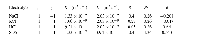
 β
 25∘C

 μD
 μr=0.01,0.1,0.5,1,10,100
 Γ0=0.024(σ0=−10.53)
 Γ0=0.01,0.02,0.03,0.05
 κa=10
 κa=30,50,100,150
 μr=0.1
 Γ∞=1nm−2(Ma=438.3)
 Ds=3.94×10⁻¹⁰m2s−1

 μD
 κa
 Γ0=0.01(σ0=−4.383)
 Γ0=0.025(σ0=−10.958)
 Γ0=0.05(σ0=−21.915)
 μr=0.01,0.1,1,10,100
 Γ∞=1nm−2(Ma=438.3)
 kd=0
 δΓ=0
 δΓ≠0
 μr
 Ds=10−9m2s−1
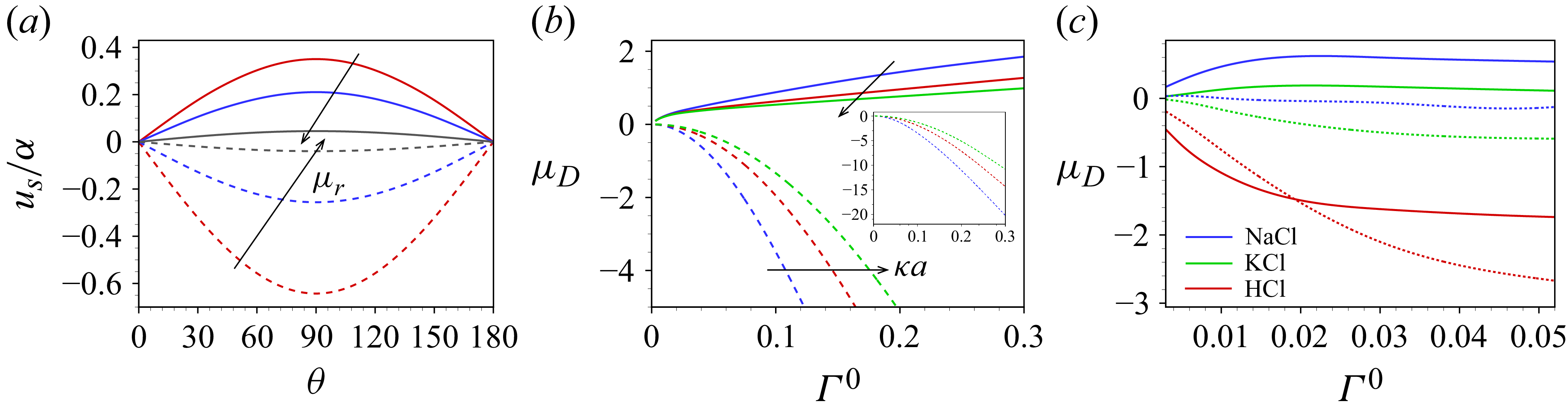
 κa=3
 Γ0=0.01
 μr=0.01,1,10
 μD
 Γ0
 κa=50,100,150
 μr=0.1
 μD
 Γ0
 κa=1
 μr=0.1
 Γ∞=1nm−2(Ma=438.3)
 kd=0
 Ds=10−9m2s−1
 δΓ=0
 δΓ≠0
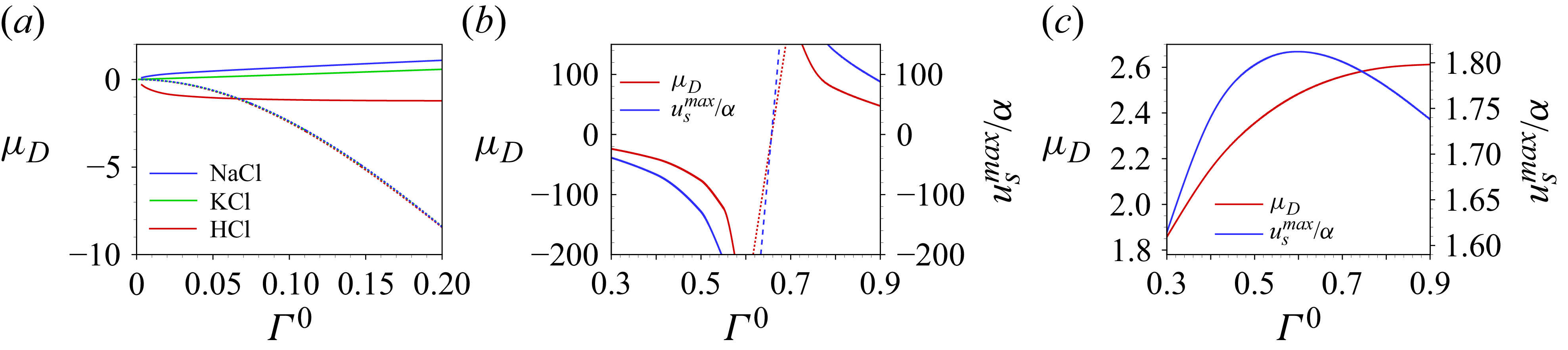
 μD
 Γ0
 κa=80
 μr=0.1
 μD
 usmax(=us|θ=π/2)
 Γ0(⩾0.3)
 κa=50
 μr=0.01
 δΓ=0
 δΓ≠0
 Γ∞=1nm−2(Ma=438.3)
 kd=0
 Ds=10−9m2s−1
 δΓ=0
 δΓ≠0
 us
 μD
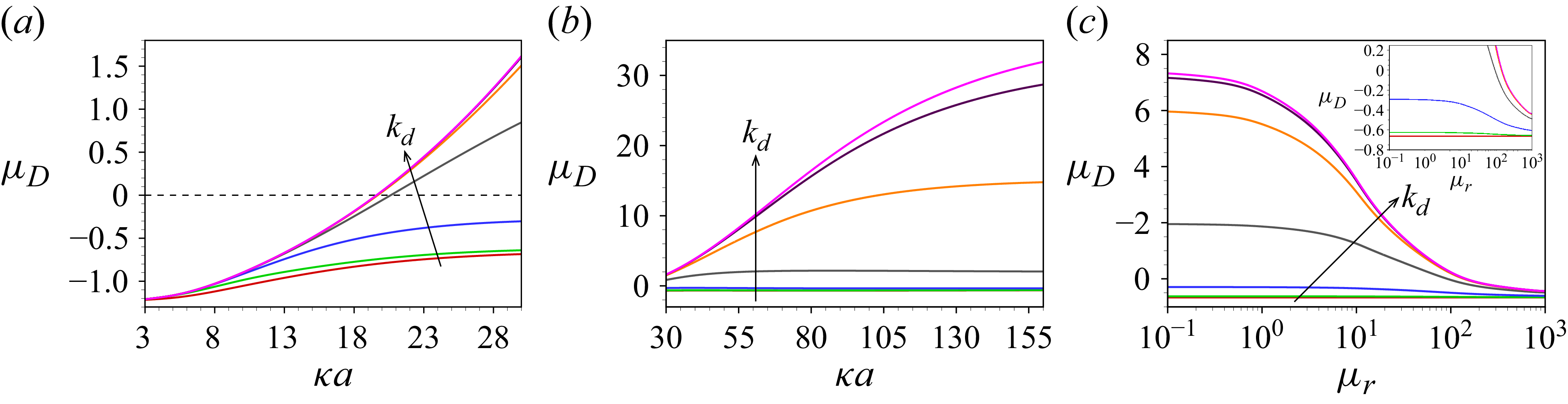
 μD
 κa
 ⩽
 κa
 ⩾
 kd=0,104,105,106,107,108,1010s−1
 μr=1
 Γ0=0.4
 μD
 μr
 kd=0,104,105,106,107,108,1010s−1
 κa=50
 Γ0=0.4
 Γ∞=1nm−2
 +
 −
 β=0.543
 μD=0

 δΓ
 κa=90
 μr=1
 Γ0=0.4
 kd=0,104,105,
 106s−1
 kd=0,104,105,106,107,108,1010s−1
 Γ∞=1nm−2
 +
 −
 β=0.543
 ΣE=−zsMaΓ0Ψ(1)αsinθ
 ΣM=Ma(1−Γ0)−1Δsαsinθ
 us=hrαsinθ
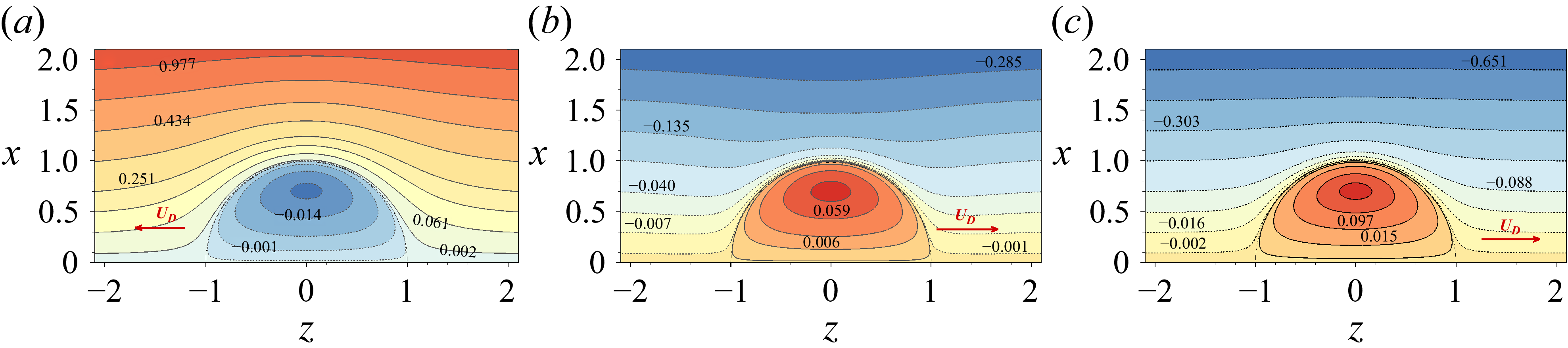
 κa=5
 μr=0.1
 kd=104s−1
 kd=106s−1
 kd=108s−1
 Γ∞=1nm−2
 Γ0=0.02
 α
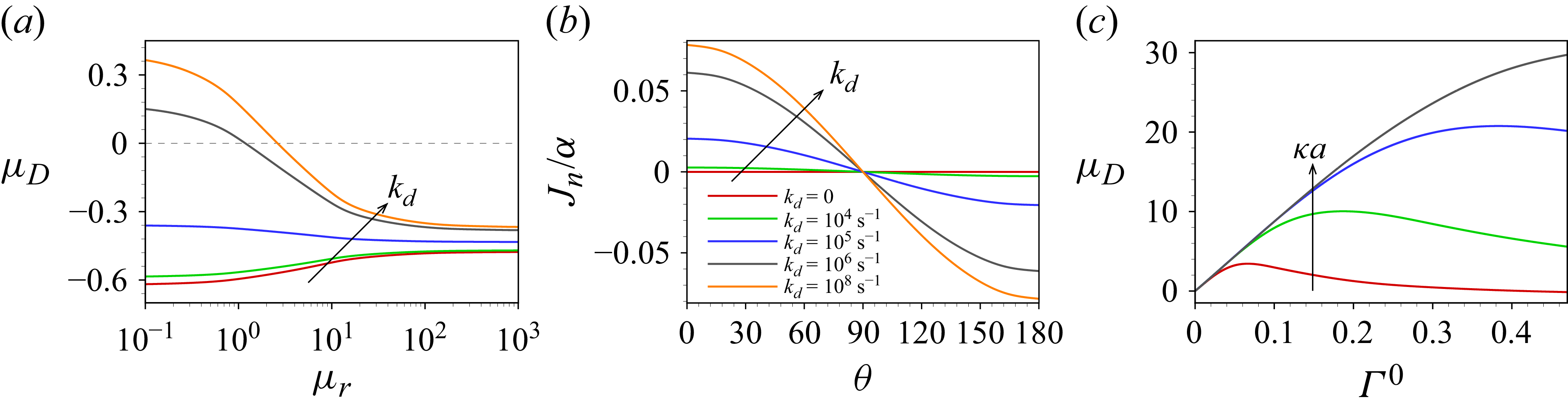
 μD
 μr
 Jn
 μr=0.1
 kd=0,104,105,106,108s−1
 κa=5
 Γ0=0.02
 μD
 Γ0
 κa=20,50,100,150
 μr=1
 kd=108s−1
 Γ∞=1nm−2
 +
 −
 β=0.543

 κa=5
 kd=3×10⁵s−1
 μr=0.1
 μr=1
 μr=10
 Γ∞=1nm−2
 Γ0=0.02
 α

 μD
 κa=20
 C~∞=15.1mM
 κa=50
 C~∞=94.7mM
 δ
 μD
 δ
 κa=50
 kd=0,104,105,106,107,108,1010s−1
 μr=1
 Γ0=0.3
 Γ∞=1nm−2
 −
 δ
 μD
 β
 δ

 δ
 κa=50
 kd=0,104,105,106,107,108s−1
 μr=1
 Γ0=0.3
 Γ∞=1nm−2
 −
 θ
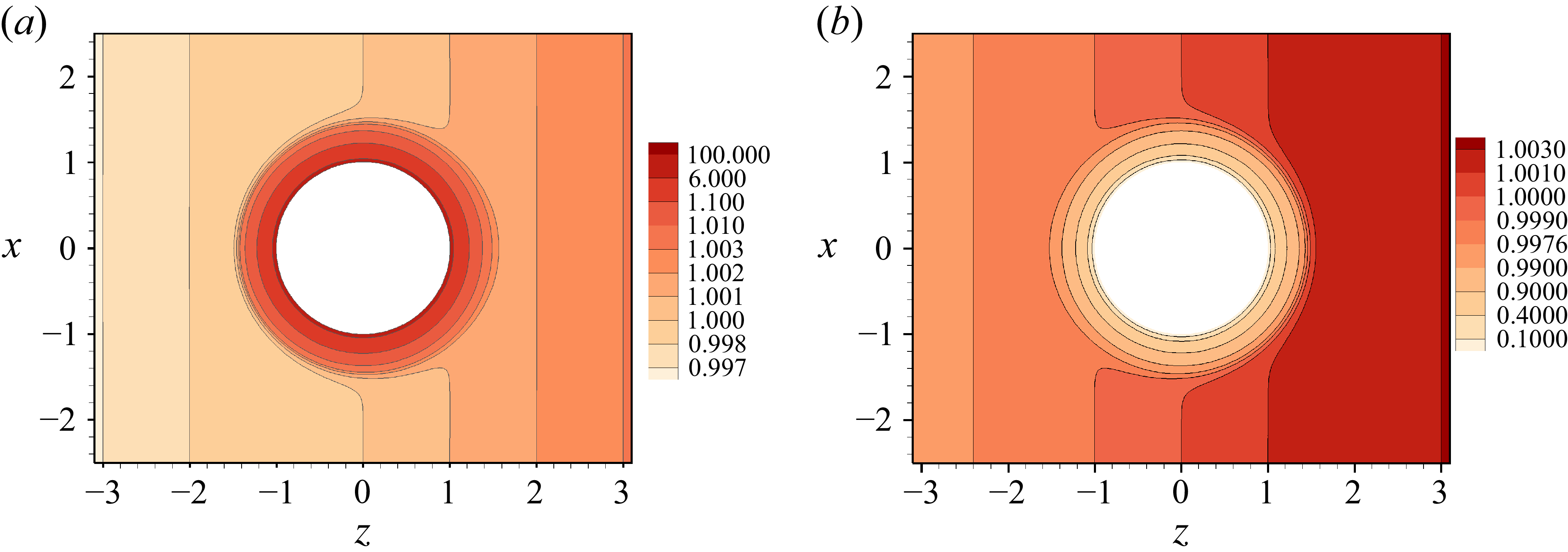
 +
 −
 κa=15
 Γ0=0.4
 μr=1
 kd=1010s−1
 Γ∞=1nm−2
 +
 −
 α=10−3
 UD∗
 +
 −
 PeNa=1.9×10⁻⁴
 PeDS=6.6×10⁻⁴

 Open access

