1 Introduction
Essential to the study of sediment transport is the criterion for onset of erosion, as it defines the threshold conditions for the initiation of sediment motion, also known as incipient motion, and is often used to set a lower bound in models to predict the transport of sediment particles. The prediction of such erosion onset to describe the threshold of bed mobility has attracted many researchers in the past (Bagnold Reference Bagnold1966; Fredsøe & Deigaard Reference Fredsøe and Deigaard1992; Sleath Reference Sleath1995; Cheng & Chiew Reference Cheng and Chiew1998; Flores & Sleath Reference Flores and Sleath1998; Sleath Reference Sleath1999; Nelson et al. Reference Nelson, Schmeeckle, Shreve and McLean2000; Papanicolaou et al. Reference Papanicolaou, Diplas, Evaggelopoulos and Fotopoulos2002; Cheng & Law Reference Cheng and Law2003; Nino, Lopez & Garcia Reference Nino, Lopez and Garcia2003; Wu & Chou Reference Wu and Chou2003; Wu & Kuo-Hsin Reference Wu and Kuo-Hsin2004; Hofland & Battjes Reference Hofland and Battjes2006).
These flows are typically turbulent in nature, and to study the dynamics of particle-bed mobility, it is important to understand the complex interactions between turbulence and sediment grains. Turbulent flow induces fluctuating forces on the particle bed, which, if they exceed a critical threshold, can strip the particles off the bed, suspend them in the fluid and deposit them elsewhere. Furthermore, Diplas and co-workers (Diplas et al. Reference Diplas, Dancey, Celik, Valyrakis, Greer and Akar2008; Celik et al. Reference Celik, Diplas, Dancey and Valyrakis2010; Valyrakis et al. Reference Valyrakis, Diplas, Dancey, Greer and Celik2010; Celik, Diplas & Dancey Reference Celik, Diplas and Dancey2013) introduced the concept of impulse and indicated that, along with the temporal bursts in drag or lift forces above a critical threshold, the duration over which they act is also critical in predicting the onset of erosion. On the other hand, the presence of particles is also seen to greatly affect the structure of the near-bed turbulence, indicated by increased bed shear stress, reduction in the near-bed anisotropy and marked changes in turbulent energy transport mechanisms (Krogstad, Antonia & Browne Reference Krogstad, Antonia and Browne1992; Krogstad & Antonia Reference Krogstad and Antonia1994; Krogstad et al. Reference Krogstad, Andersson, Bakken and Ashrafin2005; Ikeda & Durbin Reference Ikeda and Durbin2007; Chan-Braun, Garcia-Villalba & Uhlmann Reference Chan-Braun, Garcia-Villalba and Uhlmann2011; Kempe, Vowinckel & Fröhlich Reference Kempe, Vowinckel and Fröhlich2014; Yuan & Piomelli Reference Yuan and Piomelli2014; Ghodke, Apte & Urzay Reference Ghodke, Apte and Urzay2014a ; Ghodke, Skitka & Apte Reference Ghodke, Skitka and Apte2014b ; Ghodke Reference Ghodke2016; Ghodke & Apte Reference Ghodke and Apte2014, Reference Ghodke and Apte2016a ,Reference Ghodke and Apte b ,Reference Ghodke and Apte c , Reference Ghodke and Apte2017, Reference Ghodke and Apte2018). As a result of interdependence, the prediction of erosion onset, therefore, often requires linking of destabilizing hydrodynamic forces on the particle bed to the turbulent motion of the fluid around it.
Several studies have been reported to date that provide an indirect estimation of hydrodynamic forces on the particle bed using local pressure measurements (Rosenthal & Sleath Reference Rosenthal and Sleath1986; Hofland, Battjes & Booij Reference Hofland, Battjes and Booij2005; Hofland & Battjes Reference Hofland and Battjes2006; Schmeeckle, Nelson & Shreve Reference Schmeeckle, Nelson and Shreve2007; Detert, Weitbrecht & Jirka Reference Detert, Weitbrecht and Jirka2010; Dwivedi, Melville & Shamseldin Reference Dwivedi, Melville and Shamseldin2010; Amir, Nikora & Stewart Reference Amir, Nikora and Stewart2014). However, owing to the experimental difficulties, the detailed spatial structure and temporal characteristics of the fluctuating hydrodynamic forces on the particle bed still remain elusive. Recently, Chan-Braun et al. (Reference Chan-Braun, Garcia-Villalba and Uhlmann2011) and Chan-Braun, Garcia-Villalba & Uhlmann (Reference Chan-Braun, Garcia-Villalba and Uhlmann2013) reported spatio-temporal characteristics of particle forces in a unidirectional steady open-channel flow in the low-Reynolds-number regime by means of direct numerical simulations (DNS). Although, such fully resolved simulations can provide high-fidelity data of particle forces without requiring any ad hoc models, generally they are extremely challenging and require enormous computational cost for high-Reynolds-number turbulent flows in the rough regime.
Alternative approaches for estimating particle forces to predict erosion onset include use of statistical tools. Based on theoretical derivations, statistical data of particle forces are calculated indirectly by assuming a cross-correlation with Gaussian or log-normal near-bed velocity fluctuations (Einstein Reference Einstein1950; Cheng & Chiew Reference Cheng and Chiew1998; Papanicolaou et al. Reference Papanicolaou, Diplas, Evaggelopoulos and Fotopoulos2002; Cheng & Law Reference Cheng and Law2003; Wu & Chou Reference Wu and Chou2003; Wu & Kuo-Hsin Reference Wu and Kuo-Hsin2004; Hofland & Battjes Reference Hofland and Battjes2006). However, recent studies show that the near-bed flow dynamics, roughness effects and flow through porous regions lead to non-Gaussian velocity fluctuations, and higher-order turbulence statistics such as kurtosis and skewness are necessary for better predictions (Wu & Kuo-Hsin Reference Wu and Kuo-Hsin2004; Ghodke & Apte Reference Ghodke and Apte2016b ). Moreover, it is also unclear whether, and up to what spatial extent, such cross-correlation of forces with near-bed turbulent flow exists.
Most of the aforementioned studies pertaining to this topic are reported for unidirectional steady flows and very few numerical investigations studying oscillatory non-stationary turbulent flow representative of the coastal environment have been reported so far (Fornarelli & Vittori Reference Fornarelli and Vittori2009; Ding & Zhang Reference Ding and Zhang2010; Ghodke et al. Reference Ghodke, Apte and Urzay2014a ,Reference Ghodke, Skitka and Apte b ; Ghodke Reference Ghodke2016; Mazzuoli & Vittori Reference Mazzuoli and Vittori2016; Ghodke & Apte Reference Ghodke and Apte2014, Reference Ghodke and Apte2016a ,Reference Ghodke and Apte b ,Reference Ghodke and Apte c , Reference Ghodke and Apte2017, Reference Ghodke and Apte2018). However, none of these studies presented detailed information on spatio-temporal characteristics of the hydrodynamic forces on the particle bed in an oscillatory flow environment. The scope of the present paper is to analyse, by means of numerical experiments, the spatial structure and temporal characteristics of unsteady hydrodynamic forces on a rough bed made up of hexagonally packed fixed spherical particles. The simulations are carried out in a symmetric and sinusoidally oscillatory flow environment at Reynolds numbers in the turbulent rough regime. To study the effects of roughness size, two particle sizes of diameter 372 and 125 in wall units (the former corresponds to coarser particles while the latter represents finer sediment grains) are studied. Analysing these two sizes of particles, large particles (LP case) and relatively small particles (SP case), will help us understand the effects of roughness size on the statistics of hydrodynamic forces and will also provide characterization of the flow field in such cases. Moreover, the choice of particle diameter, especially the smaller one, is limited by enormous computational cost. However, note that the Reynolds number is large enough that both these cases fall in the turbulent rough regime. For both cases, statistical descriptions of drag and lift forces on the particle bed along with their cross-correlations with near-bed turbulent motions are reported. Based on the concept of impulse, an investigation of the critical threshold of drag and lift forces is also carried out.
The outline of the paper is as follows: the flow configuration and methodology are presented in § 2, simulation results are presented in § 3, followed by main conclusions in § 4.
2 Flow configuration
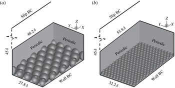
The overall flow configuration is similar to the set-up of oscillatory flow over a layer of spherical particles studied in Ghodke & Apte (Reference Ghodke and Apte2016b
). As shown in figure 1,
 $x$
,
 $y$
and
 $z$
are, respectively, the streamwise, spanwise and wall-normal directions, and
 $u$
,
 $v$
and
 $w$
are the velocity components in those directions. The computational domain, shown in figure 1, consists of a doubly periodic box in streamwise and spanwise directions. The rough bed is formed by a single layer of hexagonally packed fixed spherical particles that are touching each other. A smooth no-slip wall is located at
 $z=0$
and a slip wall at
 $z=45\unicode[STIX]{x1D6FF}$
, where
 $\unicode[STIX]{x1D6FF}=\sqrt{2\unicode[STIX]{x1D708}/\unicode[STIX]{x1D714}}$
is the Stokes layer thickness,
 $\unicode[STIX]{x1D708}$
is the kinematic viscosity,
 $\unicode[STIX]{x1D714}=2\unicode[STIX]{x03C0}/T$
is the oscillation frequency and
 $T$
is the period of the wave. In this notation, hydrodynamic force components in the streamwise
 $x$
-direction and wall-normal
 $z$
-direction are denoted as drag and lift forces, respectively. Considering an instantaneous value of the variable
 $\unicode[STIX]{x1D719}$
, its fluctuation with respect to phase and spatial average over wall-parallel planes is defined as
 $\unicode[STIX]{x1D719}^{\prime }=\unicode[STIX]{x1D719}-\langle \overline{\unicode[STIX]{x1D719}}\rangle$
. Here, the overbar and angle brackets, respectively, denote phase and homogeneous spatial averages. Note that, in the context of double averaging, the fluctuating quantity
 $\unicode[STIX]{x1D719}^{\prime }$
includes the contribution from spatial disturbance resulting from flow inhomogeneity at the roughness length scale (Ghodke & Apte Reference Ghodke and Apte2016b
).
Close-up view of the computational domain and boundary conditions for (a) LP and (b) SP cases. A harmonic pressure forcing is imposed that results in a streamwise velocity component
 $U_{\infty }\sin (\unicode[STIX]{x1D714}t)$
far from the bed.

Computational parameters and grid resolution details:
 $Re_{\unicode[STIX]{x1D6FF}}=U_{\infty }\unicode[STIX]{x1D6FF}/\unicode[STIX]{x1D708}$
is the Reynolds number based on the Stokes layer thickness,
 $Re_{a}=U_{\infty }a/\unicode[STIX]{x1D708}$
is the Reynolds number based on the wave amplitude,
 $Re_{d}=U_{\infty }d/\unicode[STIX]{x1D708}$
is the particle Reynolds number,
 $k_{s}^{+}=u_{\unicode[STIX]{x1D70F},max}k_{s}/\unicode[STIX]{x1D708}$
is the effective roughness Reynolds number and
 $d^{+}=u_{\unicode[STIX]{x1D70F},max}d/\unicode[STIX]{x1D708}$
is the particle size in wall units. Here,
 $U_{\infty }$
is the amplitude of the free-stream velocity,
 $a=U_{\infty }/\unicode[STIX]{x1D714}$
is the amplitude of the oscillation at the bed,
 $d$
is the particle diameter,
 $D=d/\unicode[STIX]{x1D6FF}$
is the particle diameter normalized by the Stokes layer thickness,
 $k_{s}\approx 2d$
is the Nikuradse roughness size and
 $u_{\unicode[STIX]{x1D70F},max}$
is the maximum friction velocity in a flow cycle. As described in Ghodke & Apte (Reference Ghodke and Apte2016b
), the value of
 $k_{s}$
was determined by fitting the double-averaged velocity profile to the logarithmic law of the wall. The maximum value of the wave friction factor,
 $f_{w,max}=2(u_{\unicode[STIX]{x1D70F},max}/U_{\infty })^{2}$
is also given. The present study assumes low Froude numbers.

The dimensionless parameters used to characterize the flow are outlined in table 1, and consist of the Reynolds number based on Stokes layer thickness,
 $Re_{\unicode[STIX]{x1D6FF}}=U_{\infty }\unicode[STIX]{x1D6FF}/\unicode[STIX]{x1D708}$
, and the effective roughness Reynolds number,
 $k_{s}^{+}=u_{\unicode[STIX]{x1D70F},max}k_{s}/\unicode[STIX]{x1D708}$
. Here,
 $U_{\infty }$
is the amplitude of the free-stream velocity,
 $k_{s}$
is the Nikuradse roughness size and
 $u_{\unicode[STIX]{x1D70F},max}$
is the maximum friction velocity in a flow cycle. The corresponding particle Reynolds number,
 $Re_{d}=U_{\infty }d/\unicode[STIX]{x1D708}$
, and the Reynolds number based on the wave amplitude,
 $Re_{a}=U_{\infty }a/\unicode[STIX]{x1D708}$
, are also given in table 1. Here,
 $a$
is the amplitude of the oscillation at the bed given by
 $a=U_{\infty }/\unicode[STIX]{x1D714}$
and
 $d$
is the particle diameter. Two sizes of particle diameter normalized by the Stokes layer thickness,
 $D=d/\unicode[STIX]{x1D6FF}$
, corresponding to the large-diameter particle (LP,
 $D=6.95$
) and the small-diameter particle (SP,
 $D=2.68$
) are studied.
Delineation of different flow regimes for oscillatory flow illustrating previous studies (Jonsson & Carlsen Reference Jonsson and Carlsen1976; Kemp & Simons Reference Kemp and Simons1982; Sleath Reference Sleath1987; Jensen, Sumer & Fredsøe Reference Jensen, Sumer and Fredsøe1989; Krstic & Fernando Reference Krstic and Fernando2001; Chen et al. Reference Chen, Chen, Tang, Stansby and Li2007; Dixen et al. Reference Dixen, Hatipoglu, Sumer and Fredsøe2008; van der A, O’Donoghue, & Davies Reference van der A, O’Donoghue, Davies and Ribberink2011) and present cases. Recent DNS (LP) cases from Ghodke & Apte (Reference Ghodke and Apte2016b ) are also shown. Encircled symbols represent present cases:

 $Re_{\unicode[STIX]{x1D6FF}}=400$
(LP);

 $Re_{\unicode[STIX]{x1D6FF}}=545$
(SP).

Figure 2 maps the different flow cases on a regime diagram (
 $a/k_{s}$
versus
 $Re_{a}$
) for oscillatory flow over roughness elements depicting the limits of laminar, transitional, smooth turbulent and rough turbulent regimes (Jensen et al.
Reference Jensen, Sumer and Fredsøe1989; van der A et al.
Reference van der A, O’Donoghue, Davies and Ribberink2011). The present cases, LP and SP, at given Reynolds numbers correspond to the very rough turbulent regime, the latter approaching the limit of the rough turbulent regime. Note that the parameters studied in this work are in the range considered by Sleath (Reference Sleath1987). For example, for the LP case,
 $\unicode[STIX]{x1D6FF}$
is around 1.17 mm,
 $U_{\infty }$
is
 $0.37~\text{m}~\text{s}^{-1}$
and the amplitude
 $a$
is around 0.24 m.
Table 1 also tabulates the flow parameters and spatial resolutions used in this study. As described in Ghodke & Apte (Reference Ghodke and Apte2016b
), uniform grids, although not cubic, are used only in the region surrounding the particles, giving roughly around 100 to 300 points in the wall-normal direction per particle diameter, and the grids are stretched in the flow normal direction above
 $z=8\unicode[STIX]{x1D6FF}~(6\unicode[STIX]{x1D6FF})$
for the LP (SP) case using hyperbolic tangent function typically used in boundary layer and channel flow calculations (Kim, Moin & Moser Reference Kim, Moin and Moser1987; Moin & Mahesh Reference Moin and Mahesh1998). Based on earlier analyses (Fornarelli & Vittori Reference Fornarelli and Vittori2009; Ghodke et al.
Reference Ghodke, Skitka and Apte2014b
) and more recent studies by Ghodke & Apte (Reference Ghodke and Apte2016b
) and Mazzuoli & Vittori (Reference Mazzuoli and Vittori2016), the present grid resolution is found to be sufficient to obtain force statistics on the given rough beds. Around
 $15$
flow cycles per case are computed to obtain statistical convergence.
As indicated in figure 1, the flow domain is around
 $48\unicode[STIX]{x1D6FF}~(56\unicode[STIX]{x1D6FF})$
long in the flow direction,
 $28\unicode[STIX]{x1D6FF}~(32\unicode[STIX]{x1D6FF})$
wide in the spanwise direction and
 $45\unicode[STIX]{x1D6FF}$
in the wall-normal direction for the LP (SP) case. Compared to Ghodke & Apte (Reference Ghodke and Apte2016b
), larger domains are used in the present study to incorporate more particles in order to obtain sufficient samples for force statistics. For both flow cases, the domain size is verified to be sufficiently large by calculating two-point spatial velocity correlation functions, in both streamwise and spanwise directions, by doubling the domain. The correlations showed no effect of domain size, and confirm the adequacy of the domain size to accommodate the largest turbulent structures (Ghodke Reference Ghodke2016; Ghodke & Apte Reference Ghodke and Apte2018). The vertical size of the domain is chosen such that all turbulent statistics decay to zero at almost half the vertical height for the high-Reynolds-number SP case under consideration.
The numerical solver based on the fictitious-domain algorithm (Apte & Finn Reference Apte and Finn2013), which facilitates solution of freely moving particles for a wide range of fluid–particle density ratios, is used, although the particles are held fixed in the present study. The solver uses a co-located grid, finite-volume, fractional time-stepping approach that is formally second-order-accurate. The numerical approach has been developed around the principles of kinetic energy conservation, especially important for high-Reynolds-number turbulent flows in complex geometries, with stretched or high-aspect-ratio grids (Apte et al.
Reference Apte, Mahesh, Moin and Oefelein2003; Mahesh, Constantinescu & Moin Reference Mahesh, Constantinescu and Moin2004; Mahesh et al.
Reference Mahesh, Constantinescu, Apte, Iaccarino, Ham and Moin2006; Apte, Mahesh & Moin Reference Apte, Mahesh and Moin2009a
; Apte et al.
Reference Apte, Mahesh, Moin and Gorokhovski2009b
). The solver is fully validated for a range of test cases, including flow over a cylinder and sphere for different Reynolds numbers, flow over touching spheres at different orientations, flow developed by an oscillating cylinder, laminar and turbulent flow through porous media, among others. The details of the numerical algorithm are presented in appendix A. Detailed verification and validation studies have been published elsewhere (Apte, Martin & Patankar Reference Apte, Martin and Patankar2008; Apte & Finn Reference Apte and Finn2013). In addition, the present configuration of oscillatory flow over a rough bed is also validated against the experimental data of Keiller & Sleath (Reference Keiller and Sleath1976) for the LP case at
 $Re_{\unicode[STIX]{x1D6FF}}=95$
, as shown in Ghodke & Apte (Reference Ghodke and Apte2016b
). In particular, variation of peak velocity magnitude and the phase at which this peak velocity is recorded, plotted at various heights above the roughness crest, are shown to agree reasonably well with the experimental work of Keiller & Sleath (Reference Keiller and Sleath1976). Other numerical predictions of parameters such as friction factor and boundary layer thickness for the LP case over a range of Reynolds numbers,
 $Re_{\unicode[STIX]{x1D6FF}}=95{-}400$
, also show good comparison with experimental data, further confirming the adequacy of the computational domain, grid resolution and rigid-body treatment (Ghodke & Apte Reference Ghodke and Apte2016b
).
For the sake of completeness, the salient flow features of fully resolved simulations of oscillatory turbulent flow in the LP case reported in Ghodke & Apte (Reference Ghodke and Apte2016b ) are summarized here. It was shown that the large particles greatly influenced near-bed turbulent structures by redistributing the energy from streamwise fluctuations to spanwise and wall-normal fluctuations, causing near-bed flow isotropization and therefore resulting in an overall reduction of large-scale anisotropy. The time-varying nature of near-bed turbulence in oscillatory flows was shown to play an important role in establishing the shape of the turbulence: the presence of two-component turbulence in the near-bed region and cigar-shaped turbulence in the outer region. Quadrant analysis revealed the dominance of sweep motions below the particle crest whereas ejection motions played an important role above the crest level. A double averaging of the flow field was also performed to reveal spatial inhomogeneities at the roughness scale resulting in alternative paths of energy transport in the turbulent kinetic energy (TKE) budget. Finally, the distributions of near-bed velocity and pressure fluctuations showed a non-Gaussian behaviour that followed a fourth-order Gram–Charlier distribution, indicating the importance of higher-order turbulence statistics in such flows.
3 Results and discussion
In this section, spatio-temporal characteristics of unsteady drag and lift forces on the particle bed are presented. To begin with, differences in the near-bed flow structures in the LP and SP cases are discussed.
3.1 Flow structures
In oscillatory flows over rough surfaces, turbulence is generated by the effects of size of the roughness and also by high-amplitude oscillations. As per Jensen et al. (Reference Jensen, Sumer and Fredsøe1989), in fully developed oscillatory turbulent flows over a rough boundary, most of the flow quantities are therefore dependent upon one single parameter, namely
 $a/k_{s}$
. As noted in table 1,
 $a/k_{s}$
in the SP case is around 3.5 times larger than that in the LP case. As a result, there exist some discernible differences in the elementary processes that govern the near-bed turbulence in the large- and the small-particle cases.
For the coarse-particle LP case,
 $a/k_{s}$
is smaller (large roughness size) compared to that for the fine-particle SP case. The size of the individual coarse particles is large enough to cause vortex shedding that is in a way also responsible for triggering the turbulence much earlier in the flow cycle (Ghodke & Apte Reference Ghodke and Apte2016b
). Contrary to this, as a result of large
 $a/k_{s}$
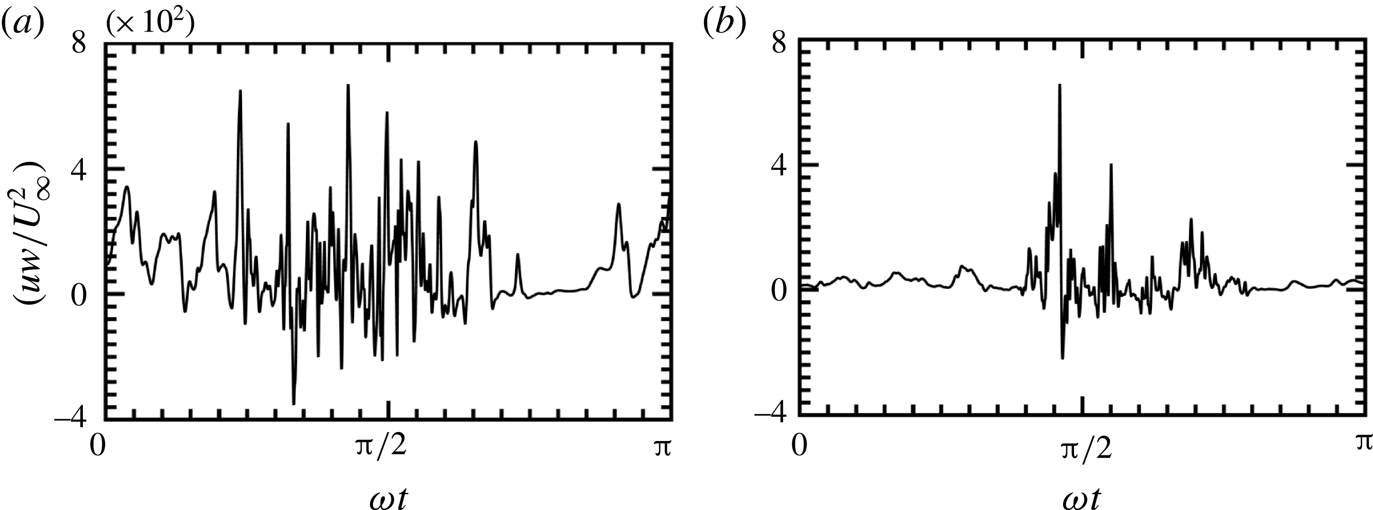
value (smaller roughness size) in the SP case, the near-bed flow exhibits an unsteady inertial behaviour in the early acceleration cycle, until the local friction velocity is large enough to trigger the turbulence. This behaviour is evident from figure 3, where the product of instantaneous streamwise (
 $u$
) and wall-normal (
 $w$
) velocity is plotted for (a) LP and (b) SP cases. The significant vortex shedding along with sweep–burst motions in the LP case result in a strong cross-correlation signal
 $uw$
from the beginning of the flow cycle. This indicates that the turbulence is present during most of the oscillation cycle for the LP case. However, as shown in figure 3(b), such cross-correlation is significant for the shear-dominated SP case only from peak phase to late deceleration phases where inertial effects play an important role in triggering the turbulence. This shows that the turbulence is present only in part of the oscillation cycle for the SP case.
Variation over a half cycle of the normalized product of instantaneous streamwise (
 $u$
) and wall-normal (
 $w$
) velocity plotted for (a) LP and (b) SP cases.

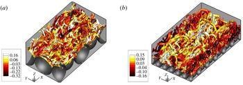
Close-up view of the instantaneous isosurfaces of the
 $\unicode[STIX]{x1D706}_{2}$
parameter coloured by
 $u^{\prime }/U_{\infty }$
for (a) LP and (b) SP cases plotted at a peak phase,
 $\unicode[STIX]{x1D714}t=5\unicode[STIX]{x03C0}/10$
. The flow direction is the positive
 $x$
-direction.

To further elucidate the near-bed flow behaviour, instantaneous flow structures in the form of
 $\unicode[STIX]{x1D706}_{2}$
isosurfaces (Jeong & Hussain Reference Jeong and Hussain1995) are plotted at the peak phase in figure 4 for (a) LP and (b) SP cases. For the LP case, there exists a complex forest of highly dense near-bed structures that appear to be broken and are slightly inclined with respect to the horizontal direction. The disruption of these flow structures is a consequence of energized wall-normal velocity fluctuations in the LP case that in turn distort the streamwise structures, resulting in flow isotropization, as already discussed in Ghodke & Apte (Reference Ghodke and Apte2016b
). On the other hand, the presence of larger elongated horseshoe structures that span over more than a few particle diameters in the flow direction along with the small-scale broken structures is clearly evident in the SP case shown in figure 4(b). Contrary to the LP case, these structures appear to be less broken, suggesting a lower degree of near-bed flow isotropization in the SP case. Such near-bed structures could play a significant role in influencing spatio-temporal characteristics of hydrodynamic forces on the particle bed. Detailed quantification of the near-bed turbulence structure in the LP and SP cases is presented in Ghodke & Apte (Reference Ghodke and Apte2018).
3.2 Particle-bed force history
In the following, the nature of unsteady forces on the particle bed is analysed. The hydrodynamic force,
 $\boldsymbol{F}$
, acting on a particle is defined as
 $$\begin{eqnarray}\displaystyle & \displaystyle \boldsymbol{F}=\int _{\unicode[STIX]{x1D6E4}}\unicode[STIX]{x1D749}\boldsymbol{\cdot }\boldsymbol{n}\,\text{d}\unicode[STIX]{x1D6E4}, & \displaystyle\end{eqnarray}$$
where
 $\text{d}\unicode[STIX]{x1D6E4}$
is the unit surface area of the particle,
 $\boldsymbol{n}$
is the surface normal vector and
 $\unicode[STIX]{x1D749}$
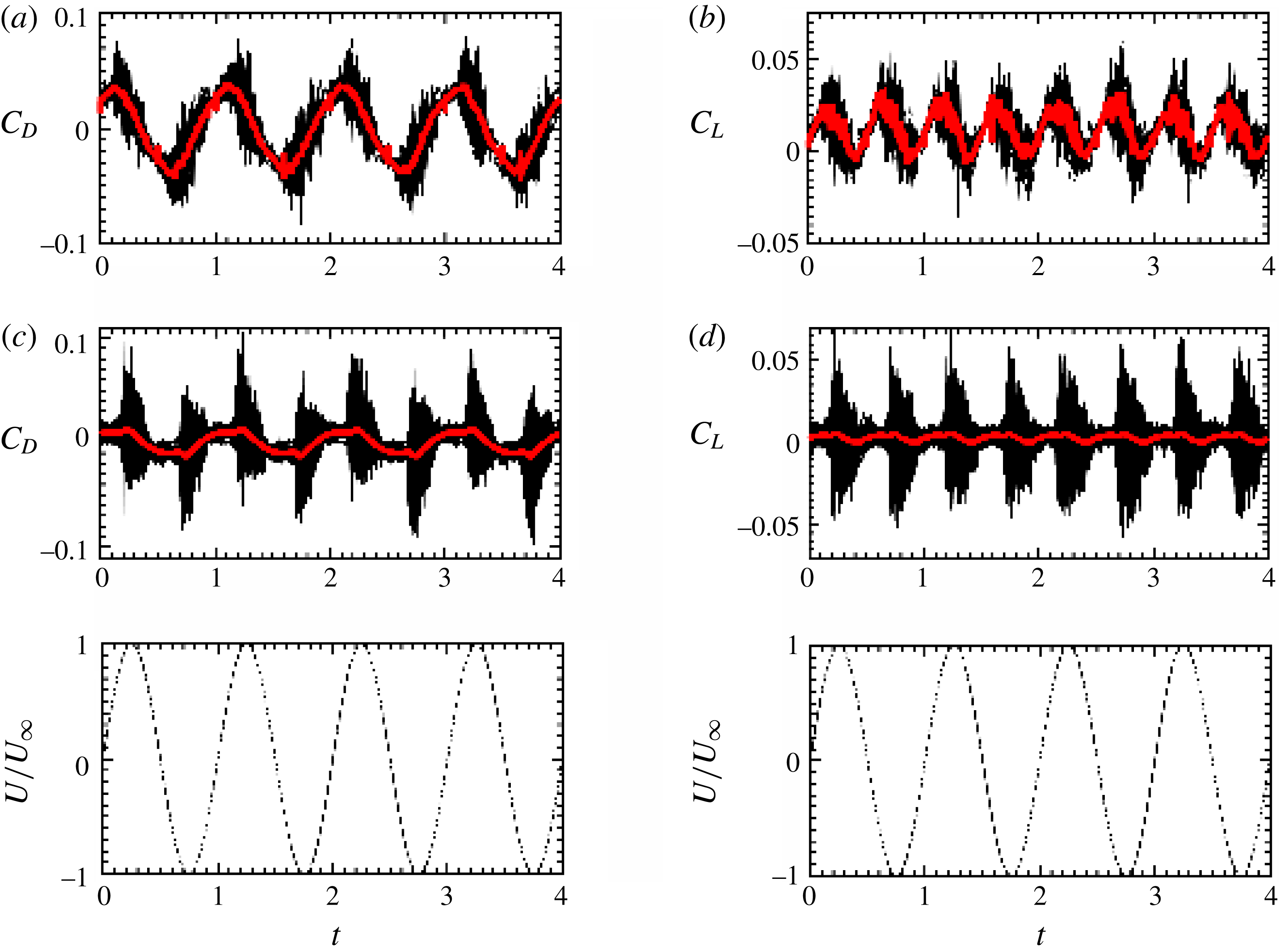
is the stress, containing both viscous and pressure contributions, on the particle surface. Figure 5 shows the phase variation of instantaneous drag (
 $C_{D}$
) and lift (
 $C_{L}$
) force coefficients on each particle (thin black lines) plotted along with the respective average force coefficients on the particle bed (thick red line). The force coefficient is defined as
 $C_{i}=F_{i}/(0.5\unicode[STIX]{x1D70C}A_{p}U_{\infty }^{2})$
, where
 $i$
stands for drag or lift with
 $F$
as the respective force and
 $A_{p}$
is the projected area of the particle. For the purpose of illustration, data for four cycles are plotted. The phase variation of the streamwise velocity far from the bed is also shown for reference. Figures 5(a) and 5(b), respectively, show the drag and lift coefficients in the LP case and figures 5(c) and 5(d) show those for the SP case. Contrary to unidirectional flows, hydrodynamic forces on the particle bed in oscillatory flows vary over a cycle. Unlike drag, the sign of the lift force is the same whether the flow is in the positive or the negative
 $x$
-direction and has a period of half the forcing function. As seen in figure 5(a,b), the variability of the instantaneous forces on each sphere from the average value is consistent throughout the entire cycle for the larger-diameter particle case. On the other hand, for the smaller-diameter particle as shown in figure 5(c,d), such variability of the instantaneous forces is significant only from late acceleration up to early deceleration phases; notably, during the same period of the oscillation cycle where the cross-correlation signal
 $uw$
is significant. Such differences in the force history for the LP and SP cases are therefore mainly a result of the different nature of the near-bed turbulence in these flow cases, as discussed earlier.
Variation over several cycles of the normalized instantaneous drag
 $C_{D}$
(a,c) and lift
 $C_{L}$
(b,d) for each particle in the flow set-up. Panels (a,b) are for the LP case and panels (c,d) are for the SP case. The thick red line indicates the average value of the force. The phase variation of the streamwise velocity far from the bed is shown (— ⋅ —) in the lowermost panels.

To further elucidate the differences in the nature of the forces for large- and small-particle cases, the phase variation of the average force on the particle bed in these flow cases is discussed in detail. Figure 6 shows the variation over a cycle of the phase-averaged drag (
 $\overline{C}_{D}$
) and lift (
 $\overline{C}_{L}$
) coefficients for the coarser (LP) and the finer (SP) roughness elements. The phase variation of the streamwise velocity far from the bed is also shown for reference. In the LP case shown in figure 6(a), both drag and lift coefficients peak earlier in the flow cycle, respectively exhibiting a phase lag of
 $\unicode[STIX]{x1D714}t=0.87$
and
 $0.34$
with the free-stream velocity. In comparison, as a result of increased Reynolds number
 $Re_{a}$
in the shear-dominated SP case, a reduced phase lag of, respectively,
 $\unicode[STIX]{x1D714}t=0.08$
and
 $0.086$
for drag and lift with the free-stream velocity is observed in figure 6(b). Note that the phase lag between the drag and lift forces also decreases as the Reynolds number is increased, as in the SP case.
Variation over a cycle of the normalized phase- and spatially averaged drag
 $\overline{C}_{D}$
(

 $\overline{C}_{L}$
(

 $\overline{C_{i}}=\langle \overline{F_{i}}\rangle /(0.5\unicode[STIX]{x1D70C}A_{b}U_{\infty }^{2})$
is the normalized phase- and spatially averaged force on the particle bed,
 $i$
stands for drag or lift, and
 $A_{b}$
is the total projected area of the particle bed. The phase variation of the streamwise velocity (not to scale) far from the bed is shown (— ⋅ —). Arrows in panel (b) indicate spikes in the drag and lift record for the SP case.

As seen in figure 6(b), there exist sharp spikes in the drag and lift records for the SP case (shown by arrows); however, such distinct spikes are absent in the LP case. As a result of significant vortex shedding along with sweep–burst motions in the LP case, there is no clear demarcation of onset of turbulence that may result in distinct spikes in the drag and lift records. Contrary to this, the occurrence of sweep–burst motions resulting in sudden transition to turbulence close to the peak velocity phase results in distinct spikes in the drag and lift records in the SP case. Note that the phase instant of these spikes in figure 6(b) clearly matches well with the occurrence of spikes in the
 $uw$
signal for the SP case shown in figure 3(b).
Force statistics for the LP and SP cases. Here,
 $\overline{C}_{D,max}$
(
 $\overline{C}_{L,max}$
) and
 $\overline{C}_{D,avg}$
(
 $\overline{C}_{L,avg}$
), respectively, show maximum and period-averaged values of the drag (lift) force coefficients over half a flow cycle; and
 $S_{D^{\prime }}$
(
 $S_{L^{\prime }}$
) and
 $K_{D^{\prime }}$
(
 $K_{L^{\prime }}$
), respectively, denote skewness and kurtosis of the drag (lift) fluctuations over half a flow cycle.

Table 2 summarizes the particle-bed force statistics for the LP and SP cases. In both flow cases, the net lift and drag coefficients remain positive and their magnitudes are decreased as the Reynolds number is increased. Higher-order moments such as skewness and kurtosis of drag/lift fluctuations over several half flow cycles are also reported in table 2. In both flow cases, the skewness values of the drag and lift forces are positive, indicating that the positive events of drag and lift are more likely to occur than the negative ones. Moreover, the high values of kurtosis of drag and lift fluctuations indicate large intermittency in the force field that results in longer tails of rare but strong events. With increase in Reynolds number (SP case) such extreme events become stronger, resulting in higher values of kurtosis. Note that kurtosis values in the SP case are almost twice as large as in the LP case. Such extreme force events might play an important role in destabilizing the particle bed. Similar observations were reported by Chan-Braun et al. (Reference Chan-Braun, Garcia-Villalba and Uhlmann2011) in their study of unidirectional flow over a rough bed.
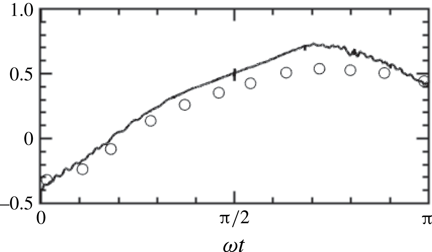
In addition, the present results of the LP case are compared against data from Mazzuoli & Vittori (Reference Mazzuoli and Vittori2016). Figure 7 shows a comparison of normalized phase- and spatially averaged drag force for
 $Re_{\unicode[STIX]{x1D6FF}}=400$
(LP) case with the data from Mazzuoli & Vittori (Reference Mazzuoli and Vittori2016). As shown in figure 7, the present results compare reasonably well with Mazzuoli & Vittori (Reference Mazzuoli and Vittori2016), albeit some discrepancies are seen in the magnitude of the force in the decelerating part of the cycle. This could be due to fewer flow cycles (only three) being considered by Mazzuoli & Vittori (Reference Mazzuoli and Vittori2016) as against 15 flow cycles in the present investigation. Nevertheless, the overall phase variation of the average force, including the phase of the peak force, in the present case matches fairly well with Mazzuoli & Vittori (Reference Mazzuoli and Vittori2016).
Variation over a half cycle of the normalized phase- and spatially averaged drag force for
 $Re_{\unicode[STIX]{x1D6FF}}=400$
(LP) case. Data from Mazzuoli & Vittori (Reference Mazzuoli and Vittori2016) are shown by symbols. Here, force is normalized by
 $\unicode[STIX]{x1D70C}U_{\infty }^{2}\unicode[STIX]{x1D6FF}^{2}$
.

3.3 Spatial distribution of the forces
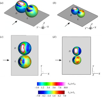
After studying the phase variation of the drag/lift forces, their distribution on the particle surface needs to be investigated. Figure 8 shows the spatial distribution at a peak phase of drag and lift components,
 $\bar{\unicode[STIX]{x1D70F}}_{D}$
and
 $\bar{\unicode[STIX]{x1D70F}}_{L}$
, respectively, of the phase-averaged stress (
 $\bar{\unicode[STIX]{x1D749}}$
) on the particle surface. Here,
 $\bar{\unicode[STIX]{x1D70F}}_{D}=\bar{\unicode[STIX]{x1D749}}\boldsymbol{\cdot }\boldsymbol{e}_{1}$
and
 $\bar{\unicode[STIX]{x1D70F}}_{L}=\bar{\unicode[STIX]{x1D749}}\boldsymbol{\cdot }\boldsymbol{e}_{3}$
, where
 $\boldsymbol{e}_{1}$
and
 $\boldsymbol{e}_{3}$
are unit vectors in the
 $x$
- and
 $z$
-directions, respectively. Figure 8(a,b) shows isometric views and figure 8(c,d) presents top views of the particles. Figures 8(a,c) and 8(b,d) show the stress distributions on the large and small particles, respectively. Note that
 $\bar{\unicode[STIX]{x1D70F}}_{D}$
and
 $\bar{\unicode[STIX]{x1D70F}}_{L}$
plotted in figure 8 indicate phase- and spatially averaged stresses. Therefore, the spheres shown in this figure do not represent a particular particle but rather show an averaged stress field on any particle in the set-up. From the variation of forces plotted in figure 6, it can be seen that the average drag/lift forces on the particle at the peak phase in both flow cases are positive. However, as shown in figure 8, local stress components contributing to drag and lift can be either positive or negative depending on the direction of the local velocity near the particle surface.
Spatial distribution of the phase- and spatially averaged local stress on the particle surface corresponding to drag,
 $\bar{\unicode[STIX]{x1D70F}}_{D}$
, and lift,
 $\bar{\unicode[STIX]{x1D70F}}_{L}$
, at a peak phase normalized by their respective standard deviations for the LP (a,c) and the SP (b,d) cases. Here,
 $D$
and
 $L$
, respectively, denote drag- and lift-related stress components. The direction of the flow is indicated by an arrow. The sizes of the particles are not to scale.

For both flow cases, there exists a region of strong positive drag component of the stress,
 $\bar{\unicode[STIX]{x1D70F}}_{D}$
, near the top of the sphere, a result of maximum strain in the streamwise velocity component at this location. In addition, small patches of weak positive
 $\bar{\unicode[STIX]{x1D70F}}_{D}$
are also found especially in the front and aft region of the large particle as shown in figure 8(a,c). These local regions of weak drag are a consequence of pore-scale flow features and are dominant mainly for the large particle due to pronounced curvature effects; however, they are clearly absent in the small-particle case shown in figure 8(b,d). Furthermore, variation of
 $\bar{\unicode[STIX]{x1D70F}}_{D}$
in the wall-normal direction reveals the location of the effective level at which the bulk drag force is exerted, also called the zero-displacement plane. In the present study, this zero-displacement plane is found to be located at
 $0.7D$
(
 $0.85D$
) for LP (SP) case. This further indicates that the total drag force is distributed on a larger area of the upper hemisphere of the large-diameter particle compared to that in the case of the small-diameter particle.
The spatial distribution of the lift component of the stress,
 $\bar{\unicode[STIX]{x1D70F}}_{L}$
, also shows some discernible differences between the LP and the SP case. As shown in figure 8(b,d), a region of positive magnitude of
 $\bar{\unicode[STIX]{x1D70F}}_{L}$
is seen mostly in the top portion of the upper hemisphere of the small-diameter particle and is a result of lower values of pressure due to flow acceleration near the particle crest. On the other hand, the
 $\bar{\unicode[STIX]{x1D70F}}_{L}$
distribution in the case of the large-diameter particle shows larger positive magnitudes on the side and aft region of the particle as shown in figure 8(a,c). This could again be attributed to the combined effects of enhanced three-dimensionality of the boundary layer, shielding effects in a hexagonal arrangement of the particles along with the complex pore-scale flow resulting from broken near-bed structures in the gaps between the particles. As a result, lower-pressure regions are mainly observed on the side and aft portion of the large-diameter particle that contribute positively to the lift. In comparison to the SP case, these effects are more pronounced for the large-diameter case due to strong curvature effects.
3.4 Temporal correlations of the forces
In the following, temporal characteristics of the force fluctuations in the LP and SP cases are studied. The time scales of drag and lift fluctuations in both flow cases are obtained from their respective temporal autocorrelations. In addition, cross-correlation of drag and lift fluctuations is also reported to reveal their interdependence on each other.
Following Chan-Braun et al. (Reference Chan-Braun, Garcia-Villalba and Uhlmann2013), the three-dimensional correlation function given as
 $$\begin{eqnarray}\displaystyle \displaystyle & & \displaystyle R_{\unicode[STIX]{x1D719}^{\prime }\unicode[STIX]{x1D713}^{\prime }}(\unicode[STIX]{x0394}x,\unicode[STIX]{x0394}y,z,\unicode[STIX]{x0394}t)\nonumber\\ \displaystyle & & \displaystyle \quad =\frac{1}{N_{c}N_{p}}\mathop{\sum }_{i=1}^{N_{c}}\mathop{\sum }_{j=1}^{N_{p}}\unicode[STIX]{x1D719}^{\prime }(x_{p,j},y_{p,j},z,t_{i})\,\unicode[STIX]{x1D713}^{\prime }[(x_{p,j}+\unicode[STIX]{x0394}x),(y_{p,j}+\unicode[STIX]{x0394}y),z,(t_{i}+\unicode[STIX]{x0394}t)]\end{eqnarray}$$
is defined, where the sub-index
 $p$
refers to the particle position, and
 $N_{p}$
and
 $N_{c}$
are the number of particles and flow cycles, respectively. Using this function, temporal autocorrelation at zero spatial separation can be calculated by setting
 $\unicode[STIX]{x1D719}^{\prime }=\unicode[STIX]{x1D713}^{\prime }$
and
 $\unicode[STIX]{x0394}x=\unicode[STIX]{x0394}y=0$
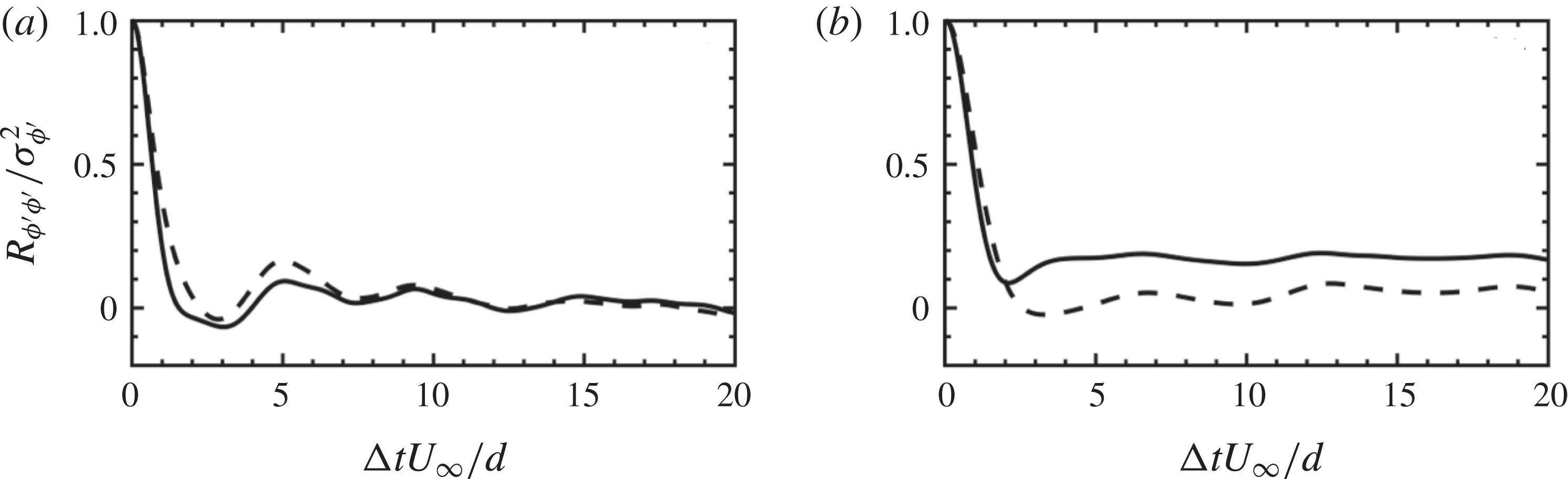
in (3.2). Figure 9 shows the variation of the autocorrelation function of drag and lift fluctuations for (a) LP and (b) SP cases.
Temporal autocorrelation of drag (——) and lift (- - - -) fluctuations for (a) LP and (b) SP plotted as a function of separation in time. Only a small fraction of the signal in which non-negligible correlation exists is plotted.

In the case of LP, autocorrelation functions for drag and lift exhibit local minima of small negative values (drag,
 $-0.066$
at
 $\unicode[STIX]{x0394}tU_{\infty }/d=3.05$
; and lift,
 $-0.039$
at
 $\unicode[STIX]{x0394}tU_{\infty }/d=2.87$
). For the SP case, the local minimum in the drag takes a positive value (
 $0.087$
at
 $\unicode[STIX]{x0394}tU_{\infty }/d=2.1$
) and that for the lift takes a negative value (
 $-0.023$
at
 $\unicode[STIX]{x0394}tU_{\infty }/d=3.3$
). Chan-Braun et al. (Reference Chan-Braun, Garcia-Villalba and Uhlmann2013), in their DNS study of unidirectional flow over a rough bed, also observed such local minima in drag/lift autocorrelations. They argued that the minimum peak in drag/lift autocorrelations might be linked to the effects of pressure; a result analogous to the pronounced minimum of negative value of pressure autocorrelation on a smooth wall in a turbulent channel flow. The present results also show similar trends; however, the values of the local minima are typically 3–4 times smaller than those reported by Chan-Braun et al. (Reference Chan-Braun, Garcia-Villalba and Uhlmann2013). It should be noted that the unidirectional flow study reported by Chan-Braun et al. (Reference Chan-Braun, Garcia-Villalba and Uhlmann2013) falls in the hydrodynamically smooth and transitional regime, whereas the Reynolds numbers in the present cases are dramatically higher and fall in the very rough turbulent regime.
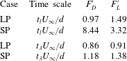
Using the temporal autocorrelation function, two different time scales, integral (
 $t_{l}$
) and Taylor micro-scale (
 $t_{\unicode[STIX]{x1D706}}$
), for drag and lift fluctuations are calculated. The integral time scale, defined as the integral of the autocorrelation, is computed in the integration domain within which the value of the autocorrelation function monotonically decreases and goes to significantly smaller value (here,
 $\unicode[STIX]{x0394}tU_{\infty }/d\in [0,20]$
). The short-time behaviour of the autocorrelation function can be quantified using the Taylor micro-scale (
 $t_{\unicode[STIX]{x1D706}}$
), defined by the zero crossing of the parabola osculating the correlation function at zero separation.
Table 3 tabulates integral time scales and temporal Taylor micro-scales of drag/lift fluctuations for the LP and SP cases. The following observations could be noted by comparing these two cases: (i) The integral time scales of force fluctuations for the LP case are typically smaller than those for the SP case. This could be attributed to the different nature of the near-bed turbulence in these flow cases. The broken streamwise structures of the time scale
 ${\sim}d/U_{\infty }$
in the LP case are responsible for inducing drag/lift fluctuations on the large-diameter particle, resulting in integral time scales almost close to unity. On the contrary, the presence of elongated streamwise structures of the size of several particle diameters results in larger values of integral time scales of force fluctuations in the SP case. (ii) As a result of significant flow isotropization, the Taylor micro-scales of drag/lift fluctuations for the large-diameter particle are almost comparable to their integral time scales, suggesting the absence of disparity in time scales. In the SP case, small-scale drag/lift fluctuations are dominated by small-scale turbulent motions of the time scale
 ${\sim}d/U_{\infty }$
, typically resulting in Taylor micro-scales of the order of unity. In general, these results indicate that the small-diameter particle typically exhibits force fluctuations of longer duration than those of the large-diameter particle case under investigation.
Integral time scale (
 $t_{l}$
) and temporal Taylor micro-scale (
 $t_{\unicode[STIX]{x1D706}}$
) of drag and lift fluctuations for the LP and SP cases. The time scales are non-dimensionalized using
 $d/U_{\infty }$
.

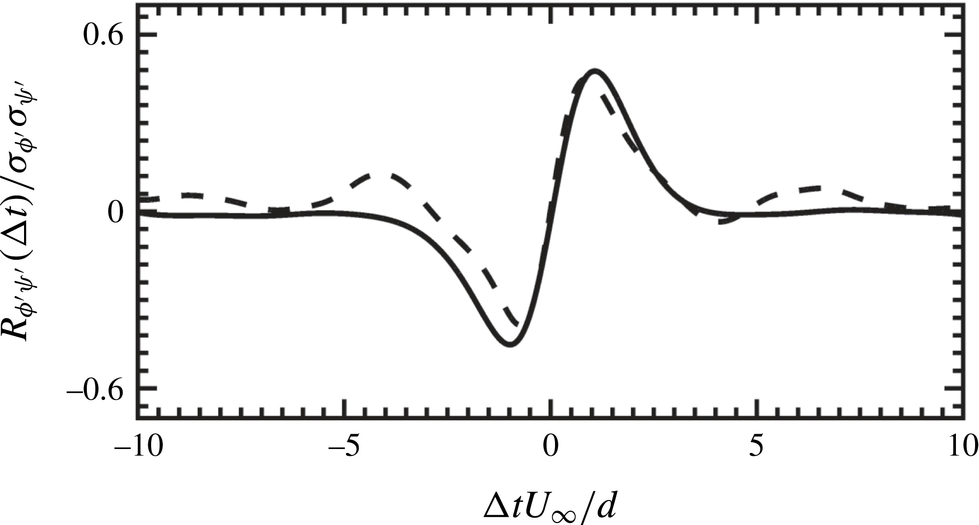
To further understand the behaviour of particle-bed forces, the temporal cross-correlation function of the drag and lift fluctuations is computed. This would help to investigate if drag and lift fluctuations are correlated in time and are affected by similar near-bed flow structures. Phase-averaged cross-correlation is calculated by setting
 $\unicode[STIX]{x1D719}^{\prime }=F_{D}^{\prime }$
,
 $\unicode[STIX]{x1D713}^{\prime }=F_{L}^{\prime }$
and
 $\unicode[STIX]{x0394}x=\unicode[STIX]{x0394}y=0$
in (3.2) and is plotted in figure 10. For no shift in time (
 $\unicode[STIX]{x0394}t=0$
), the cross-correlation is very small and the drag and lift fluctuations are weakly correlated. The cross-correlation reaches a maximum value
 $0.45$
(
 $0.48$
) for separation in time
 $\unicode[STIX]{x0394}tU_{\infty }/d=0.86$
(
 $1.08$
) for LP (SP) case, indicating that the drag and lift fluctuations, on average, are positively correlated with each other. This suggests that the positive fluctuation in the drag (result of stagnation pressure) corresponds to the simultaneous positive fluctuation in the lift. It is also interesting to note that the time lag of the maximum value of the correlation function approximately matches the Taylor micro-scale of the drag and lift fluctuations (cf. table 3). Furthermore, as shown in figure 10, the cross-correlation takes the minimum value
 $-0.39$
(
 $-0.45$
) for separation in time
 $\unicode[STIX]{x0394}tU_{\infty }/d=-0.73$
(
 $-0.98$
) for LP (SP) case. For larger negative separation times, the correlation function for the LP and SP cases increases from a minimum value to reach zero. In comparison to previous unidirectional flow studies (Hofland Reference Hofland2005; Dwivedi Reference Dwivedi2010; Chan-Braun et al.
Reference Chan-Braun, Garcia-Villalba and Uhlmann2013; Amir et al.
Reference Amir, Nikora and Stewart2014), there exist significant differences in the present case in terms of flow conditions, particle Reynolds number, particle shape and arrangement, methodologies for the flow data measurements, etc. However, it is promising to see that the overall shape and the behaviour of the cross-correlation function, i.e. local maximum (minimum) for positive (negative) separation, remains identical. Also, the maximum values of the cross-correlation function between
 $0.12$
and
 $0.55$
were reported in these studies and, interestingly, the present values for the LP and SP cases also fall well within this range. Such behaviour of the cross-correlation of drag and lift fluctuations seems to be very robust and is conjectured to be the effect of a strong influence of the pressure field on the particle-bed forces. This interpretation is in favour of a model approach proposed by Hofland (Reference Hofland2005) based on a convected frozen pressure field.
Temporal cross-correlation of drag and lift fluctuations plotted as a function of separation in time for the LP (- - - -) and the SP (——) cases. Only a small fraction of the signal in which non-negligible correlation exists is plotted.

3.5 Spectra
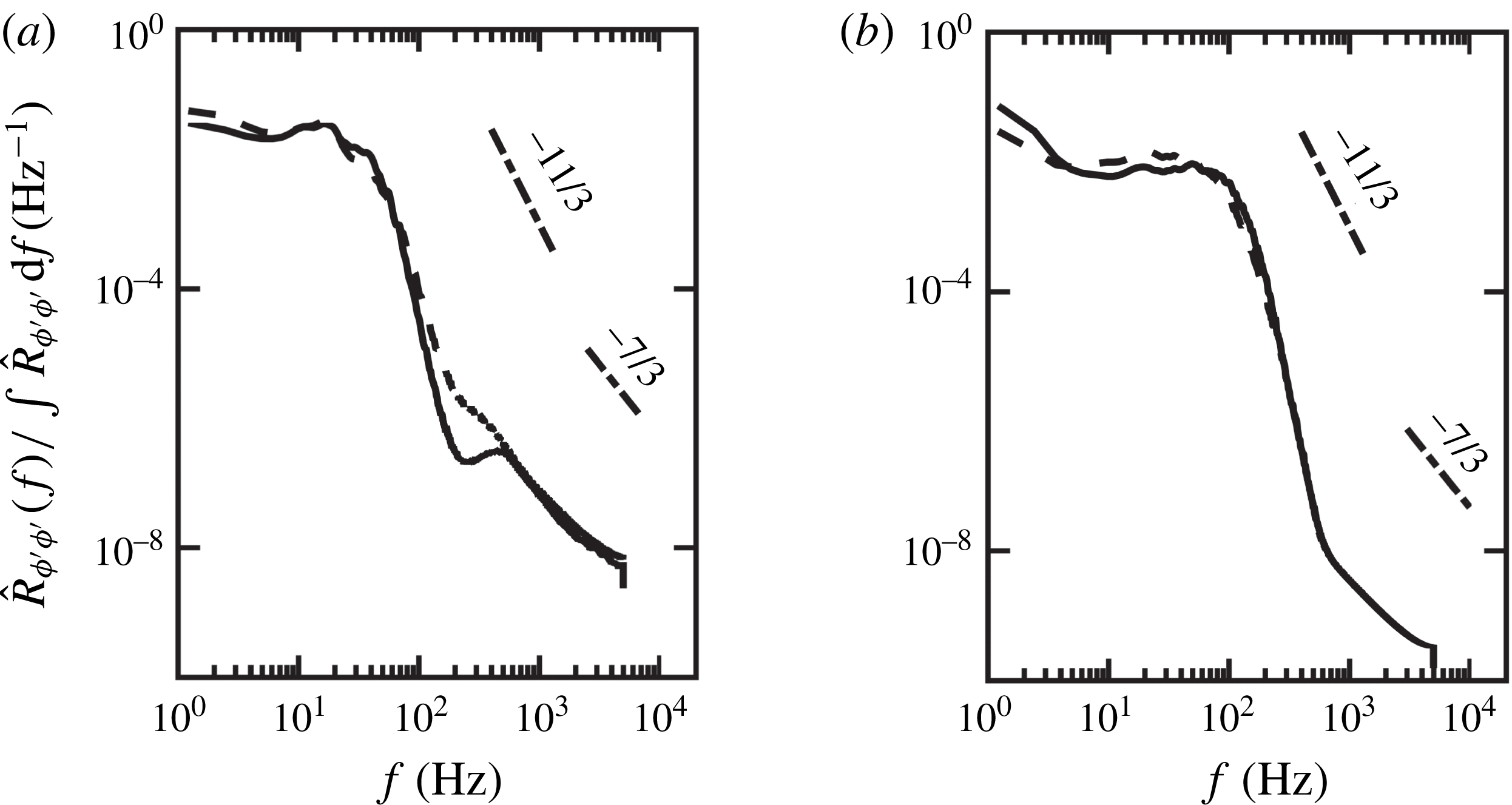
To understand the spectral content of drag and lift fluctuations, their frequency spectra
 $\widehat{R}_{\unicode[STIX]{x1D719}^{\prime }\unicode[STIX]{x1D719}^{\prime }}(f)$
are investigated. Owing to the finite nature of the signal, the modified periodogram method of Welch (Reference Welch1967) with
 $50\,\%$
overlap and applying a Hamming window to the original signal is employed. Here, spectra are averaged for all the particles and flow cycles and are normalized by the integral of spectra over all the frequencies. Figure 11 shows normalized spectra of drag (solid line) and lift (dashed line) fluctuations for (a) LP and (b) SP cases. It can be seen that, in both flow cases, a reasonably good collapse of spectra for drag and lift fluctuations is observed, with the largest spectral contributions at lower frequencies. Previously, George, Beuther & Arndt (Reference George, Beuther and Arndt1984) have performed spectral analysis of turbulent pressure fluctuations in a homogeneous constant mean-shear flow and reported the presence of
 $-11/3$
and
 $-7/3$
scaling in the pressure spectrum when turbulence–mean-shear and turbulence–turbulence interactions dominate, respectively. Interestingly, the present data for oscillatory flow over a rough bed are reminiscent of similar scalings for drag and lift fluctuations.
Spectra of drag (——) and lift (- - - -) fluctuations for (a) LP and (b) SP cases.

In comparison to the LP case, the
 $-11/3$
scaling region for the SP case extends a little further up to higher frequencies (
 ${\approx}600~\text{Hz}$
), suggesting that a wider range of scales are dominated by turbulence–mean-shear interactions. On the other hand, as a result of significant flow isotropization in the LP case, it is possible that the turbulence–turbulence interactions play an equally important role exhibiting
 $-7/3$
scaling for much higher frequencies (
 ${\approx}100~\text{Hz}$
). Recently, Hofland (Reference Hofland2005) and Detert et al. (Reference Detert, Weitbrecht and Jirka2010) in their unidirectional flow studies showed that the turbulent wall pressure spectra exhibit
 $-7/3$
scaling, whereas Amir et al. (Reference Amir, Nikora and Stewart2014) reported the presence of
 $-11/3$
scaling region. Contrary to these laboratory studies, where only pressure spectra were analysed, the present results provide spectral energy content of calculated drag and lift fluctuations. Nevertheless, it is interesting to see that the present data for the LP and SP cases typically exhibit similar behaviour as that observed in unidirectional studies. This highlights the important role of pressure, indicating the universal nature of the force fluctuations on the roughness bed.
3.6 Particle forces and turbulent flow-field correlations
The aim of this investigation is to shed light on the role of near-bed flow features that are responsible for inducing unsteady fluctuating forces on the particle bed. As noted earlier, computations or measurements of drag and lift forces on the particle bed are not straightforward. Instead, they are calculated indirectly by assuming a cross-correlation with near-bed velocity fluctuations. In this context, two questions arise: What is the distribution of the near-bed velocity? And, to what spatial extent is it cross-correlated with unsteady forces on the particle bed?
To answer the former, Ghodke et al. (Reference Ghodke, Apte and Urzay2014a ,Reference Ghodke, Skitka and Apte b ) showed the probability density function (p.d.f.) of the near-bed velocity and pressure fluctuations in the region above the particle to be non-Gaussian and to follow fourth-order Gram–Charlier distribution model given by
 $$\begin{eqnarray}\displaystyle & \displaystyle f_{GC4}(\unicode[STIX]{x1D713}^{\prime })=\frac{\text{exp}(-{\unicode[STIX]{x1D713}^{\prime }}^{2}/2)}{\sqrt{2\unicode[STIX]{x03C0}}}\left[1+\frac{S_{\unicode[STIX]{x1D713}^{\prime }}}{3!}({\unicode[STIX]{x1D713}^{\prime }}^{3}-3\unicode[STIX]{x1D713}^{\prime })+\frac{K_{\unicode[STIX]{x1D713}^{\prime }}-3}{4!}({\unicode[STIX]{x1D713}^{\prime }}^{4}-6{\unicode[STIX]{x1D713}^{\prime }}^{2}+3)\right], & \displaystyle\end{eqnarray}$$
where
 $\unicode[STIX]{x1D713}^{\prime }$
is the normalized fluctuating flow variable, and
 $S_{\unicode[STIX]{x1D713}^{\prime }}$
and
 $K_{\unicode[STIX]{x1D713}^{\prime }}$
are the skewness and flatness of its distribution, respectively.
To answer the latter, evaluation of the spatial extent of the cross-correlation between forces on the particle bed and the streamwise velocity and pressure fluctuations is carried out in a similar manner as done by Chan-Braun et al. (Reference Chan-Braun, Garcia-Villalba and Uhlmann2013) for unidirectional steady flow. To this end, the three-dimensional correlation function given by (3.2) is computed by taking
 $\unicode[STIX]{x1D719}^{\prime }$
as the local stress field corresponding to the fluctuating drag/lift force and
 $\unicode[STIX]{x1D713}^{\prime }$
as the flow variable fluctuations. As per (3.2), the correlation function
 $R_{\unicode[STIX]{x1D719}^{\prime }\unicode[STIX]{x1D713}^{\prime }}$
is averaged for all the particles and for
 $15$
flow cycles in each case. For the purpose of comparison between two roughness sizes,
 $R_{\unicode[STIX]{x1D719}^{\prime }\unicode[STIX]{x1D713}^{\prime }}$
is normalized by using maximum friction velocity
 $u_{\unicode[STIX]{x1D70F},max}$
and
 $\unicode[STIX]{x1D70C}u_{\unicode[STIX]{x1D70F},max}^{2}$
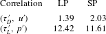
as characteristic scales for velocity and pressure fluctuations, respectively, and by using the standard deviation of the respective force fluctuations. As a result, the correlation here is not bounded by unity. The maximum values of the correlations,
 $|R_{\unicode[STIX]{x1D719}^{\prime }\unicode[STIX]{x1D713}^{\prime }}|_{max}$
, are given in table 4.
In the following, cross-correlations of the drag component of the stress with velocity fluctuations (
 $\unicode[STIX]{x1D70F}_{D}^{\prime }-u^{\prime }$
) and the lift component of the stress with pressure fluctuations (
 $\unicode[STIX]{x1D70F}_{L}^{\prime }-p^{\prime }$
) at the peak phase are presented. This choice is based on the following considerations. In the similar set-up of a closely packed bed studied by Mazzuoli & Vittori (Reference Mazzuoli and Vittori2016), the pressure contribution to the lift force was significantly larger than the viscous contribution. On the other hand, the viscous contribution (which is mainly related to the streamwise velocity) was significant and comparable to the pressure in the case of the drag force. In this context, drag (lift) is cross-correlated with velocity (pressure) fluctuations. Note that drag and lift fluctuations, on average, are positively correlated with a time lag (cf. figure 10) and therefore given correlation fields should suffice for complete description of the flow field.
Maximum amplitude of the correlation between particle force and the flow field,
 $|R_{\unicode[STIX]{x1D719}^{\prime }\unicode[STIX]{x1D713}^{\prime }}|_{max}$
, in the LP case and the SP case. Here,
 $|R_{\unicode[STIX]{x1D719}^{\prime }\unicode[STIX]{x1D713}^{\prime }}|_{max}$
is normalized by using maximum friction velocity
 $u_{\unicode[STIX]{x1D70F},max}$
and
 $\unicode[STIX]{x1D70C}u_{\unicode[STIX]{x1D70F},max}^{2}$
as characteristic scales for velocity and pressure fluctuations, respectively, and by using standard deviation of the respective force fluctuations.

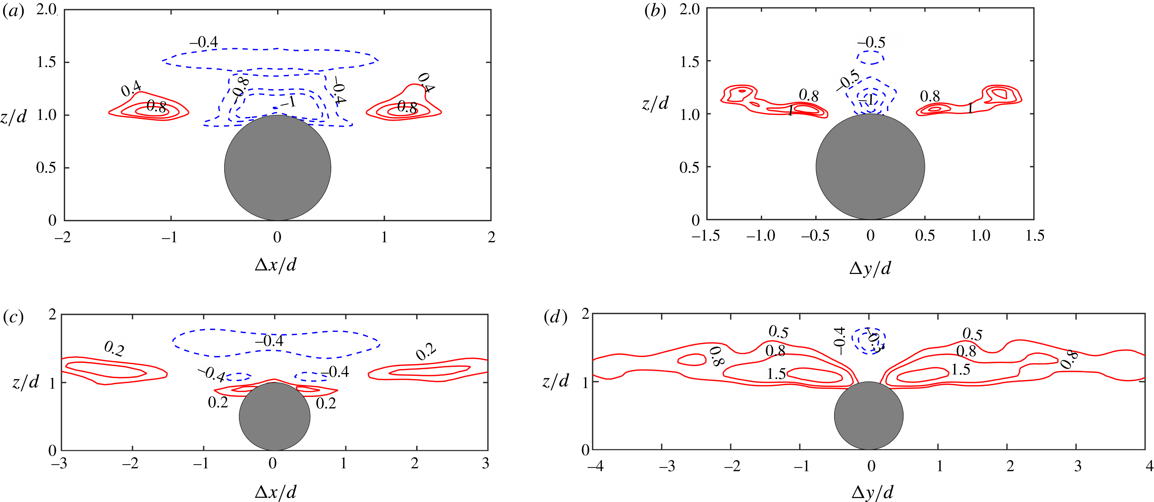
Close-up view of isocontours of correlation function
 $R_{\unicode[STIX]{x1D719}^{\prime }\unicode[STIX]{x1D713}^{\prime }}$
of drag (
 $\unicode[STIX]{x1D70F}_{D}^{\prime }$
) and streamwise velocity (
 $u^{\prime }$
) fluctuations for the LP (a,b) and the SP (c,d) cases plotted at a peak phase. Panels (a,c) show planes at zero spanwise shift (
 $\unicode[STIX]{x0394}y=0$
) and (b,d) show planes at zero streamwise shift (
 $\unicode[STIX]{x0394}x=0$
). Here, correlation is normalized by
 $u_{\unicode[STIX]{x1D70F},max}$
and standard deviation of drag fluctuations
 $\unicode[STIX]{x1D70E}_{\unicode[STIX]{x1D70F}_{D}^{\prime }}$
at a peak phase. Solid (dashed) lines indicate positive (negative) correlation.

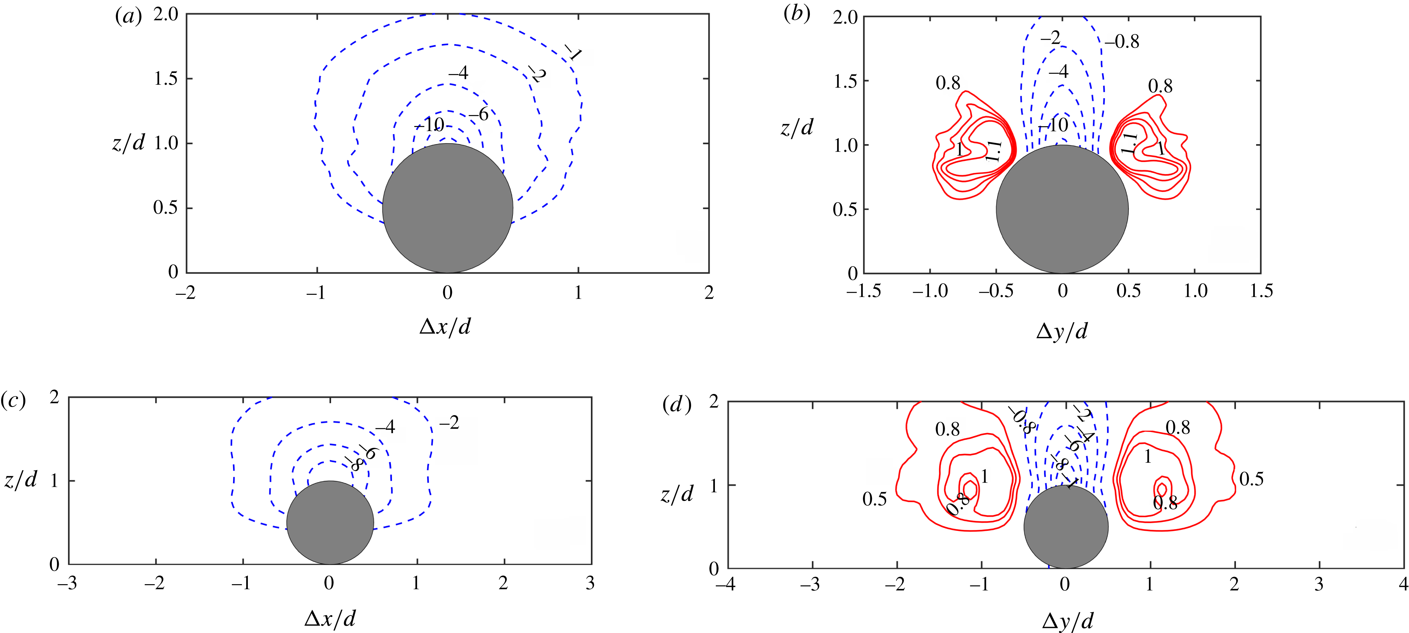
Figure 12 shows isocontours of the correlation function of the drag component of the stress and velocity fluctuations for the LP (a,b) and the SP (c,d) cases plotted at a peak phase. Planes at zero spanwise shift (
 $\unicode[STIX]{x0394}y=0$
) and zero streamwise shift (
 $\unicode[STIX]{x0394}x=0$
) are shown in figures 12(a,c) and 12(b,d), respectively. A close-up view of the domain where significant correlations exists is presented. As shown in figure 12(a), drag is positively correlated with velocity fluctuations at around one diameter distance upstream and downstream from the large-diameter particle. The spanwise view shown in figure 12(b) reveals the presence of ‘wing-shaped’ positive correlation between drag and velocity fluctuations. The presence of such a wing shape could be attributed to the complex shielding effects due to the hexagonal packing of the bed that results in disruption of the typical pattern of high-speed/low-speed streaks found in the square arrangement of particles. As shown in figure 12(c,d), a similar shape of the correlation is observed in the case of the small-diameter particle. However, in comparison to the LP case, the spatial extent of the correlation is typically 2–3 times larger in both streamwise and spanwise directions for the SP case. As discussed earlier, this could be attributed to the presence of longer near-bed flow structures found in the SP case. On the contrary, as a result of significant flow isotropization in the LP case, only local flow structures around the particle are responsible for inducing hydrodynamic forces on the particle.
As seen in figure 12(a,b), there exists a region of negative correlation between drag and velocity fluctuations just above the crest of the large-diameter particle; however, in the case of smaller particles, the correlation is positive at this location, as shown in figure 12(c). It is conjectured that such a region of negative correlation in the LP case is a result of local near-bed flow deceleration before the end of the peak phase and is typically less predominant in the high-Reynolds-number SP case, a behaviour also evident from the reduced phase lag between particle forces and outer flow as discussed in § 3.2. These effects are attributed to the oscillatory nature of the flow and were not seen in a unidirectional flow study (Chan-Braun et al. Reference Chan-Braun, Garcia-Villalba and Uhlmann2013).
Figure 13 presents isocontours of correlation function of lift component of the stress and pressure fluctuations for the LP (a,b) and the SP (c,d) cases plotted at a peak phase. The overall shape of the correlation is similar for large- and small-diameter particles. In both the cases, a negative correlation between lift and pressure fluctuations is observed in the region above the particle crest, indicating that negative fluctuation in the pressure results in positive fluctuation in the lift. This region extends up to
 $1D$
distance upstream and downstream in the streamwise direction from the large and the small particle centre as shown in figure 13(a,c). Similar to figure 12(b,d), the presence of wing-shaped positive correlation between lift and pressure fluctuations for both LP and SP cases is clearly evident in figure 13(b,d). Again, the overall shape of this correlation is comparable for the large- and small-diameter particles, although a little wider for the latter, as shown in figure 13(d). Also, as reported in table 4, it is interesting to see that the maximum values of correlation between particle forces and flow variables are almost of the same order of magnitude for both flow cases.
In summary, the presence of such regions of significant correlations between the forces on particles and the turbulent flow field around them further provides evidence of the direct link between near-bed flow structures and unsteady hydrodynamic forces on the roughness bed. The knowledge of such regions of significant correlations is beneficial and could be used to indirectly calculate the particle forces by measuring the flow variables at such locations.
Close-up view of isocontours of correlation function
 $R_{\unicode[STIX]{x1D719}^{\prime }\unicode[STIX]{x1D713}^{\prime }}$
of lift (
 $\unicode[STIX]{x1D70F}_{L}^{\prime }$
) and pressure (
 $p^{\prime }$
) fluctuations for the LP (a,b) and the SP (c,d) cases plotted at a peak phase. Panels (a,c) show planes at zero spanwise shift (
 $\unicode[STIX]{x0394}y=0$
) and (b,d) show planes at zero streamwise shift (
 $\unicode[STIX]{x0394}x=0$
). Here, correlation is normalized by
 $\unicode[STIX]{x1D70C}u_{\unicode[STIX]{x1D70F},max}^{2}$
and standard deviation of lift fluctuations
 $\unicode[STIX]{x1D70E}_{\unicode[STIX]{x1D70F}_{L}^{\prime }}$
at a peak phase. Solid (dashed) lines indicate positive (negative) correlation.

3.7 Particle force distributions
In order to further explore the possibility of influencing probabilistic models for sediment incipient motion, it would be of interest to analyse the p.d.f. of near-bed flow parameters and relate it with the hydrodynamic forces on the particles. Given the high correlation of particle forces with the near-bed flow parameters, it is expected that they follow a similar distribution as that of the velocity and pressure fluctuations. In that case, statistics of forces on the particle bed could be obtained by using the information of measurable near-bed flow variables.
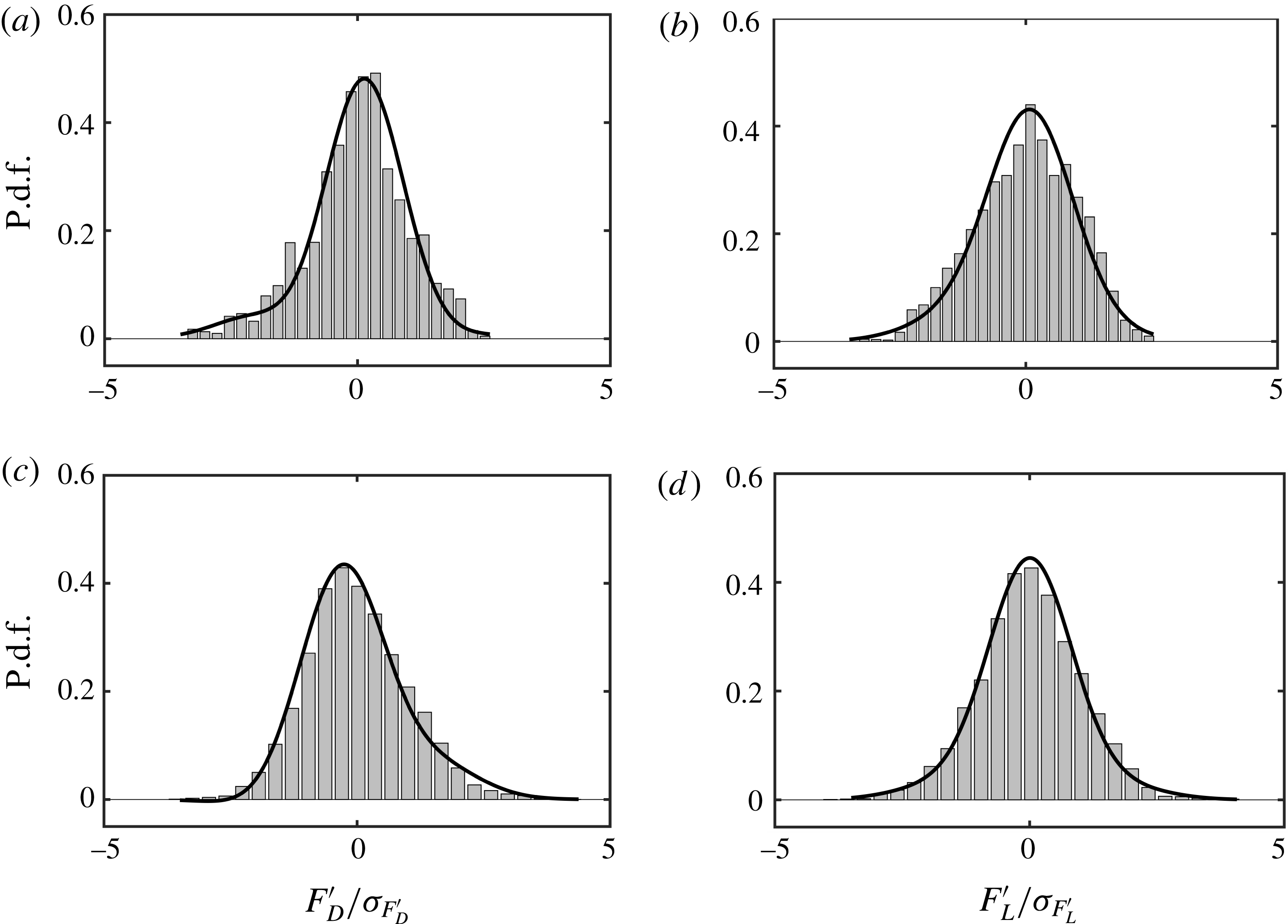
To this end, p.d.f.s of drag and lift fluctuations are constructed for the LP and SP cases. Also, pressure and velocity data are collected in the regions of high correlations as shown in figures 12 and 13, and their higher-order moments such as skewness and flatness are used to build a fourth-order Gram–Charlier distribution given by (3.3). Figure 14 shows p.d.f.s of (a,c) drag and (b,d) lift fluctuations represented by histograms for the (a,b) LP and (c,d) SP cases plotted at a peak phase. The p.d.f.s of (a,c) velocity and (b,d) pressure fluctuations constructed by using a fourth-order Gram–Charlier distribution are also plotted (solid line) in figure 14. In both cases, p.d.f.s of drag (lift) fluctuations, in particular, peakedness and long tails, match remarkably well with fourth-order Gram–Charlier distributions of velocity (pressure) fluctuations. These findings imply that the distribution of hydrodynamic forces on the particle bed is influenced by near-bed flow structures and can be constructed through higher-order flow statistics, further re-emphasizing the need to incorporate the effects of near-bed bursting and sweep phenomena into probabilistic models for onset of erosion.
P.d.f.s, normalized by standard deviations at a peak phase, of (a,c) drag (velocity) fluctuations and (b,d) lift (pressure) fluctuations represented by histograms (solid line). Panels (a,b) and (c,d) are for LP and SP cases, respectively. The p.d.f. of velocity and pressure fluctuations (solid line) is constructed by using a fourth-order Gram–Charlier distribution (3.3).

3.8 Concept of impulse
Diplas and co-workers (Diplas et al. Reference Diplas, Dancey, Celik, Valyrakis, Greer and Akar2008; Celik et al. Reference Celik, Diplas, Dancey and Valyrakis2010; Valyrakis et al. Reference Valyrakis, Diplas, Dancey, Greer and Celik2010; Celik et al. Reference Celik, Diplas and Dancey2013; Celik, Diplas & Dancey Reference Celik, Diplas and Dancey2014) introduced the concept of impulse indicating the importance of both magnitude and duration of fluctuating hydrodynamic forces on sediment erosion. Although such an approach holds promise in accounting for the intermittent dynamics of turbulent flows, there are certain difficulties in describing such a criterion. For example, detecting the peak events to calculate impulse from the time signal of a force history requires a priori specification of a threshold or a critical value of the force. It is difficult, however, to determine the correct choice of such a threshold that is best suited to predict the incipient motion. The present investigation deals with a fixed particle bed and it is not possible to detect the peak events resulting in particle erosion. Nevertheless, to shed some light on the topic, statistical analyses to provide a brief description of intermittency in fluctuating forces by means of counts and duration of peak events, impulse magnitude and their p.d.f.s for a range of threshold conditions are provided. Such characterization of force intermittency might serve as a useful tool in making a reasonable choice of a threshold criterion in future studies pertaining to this topic.
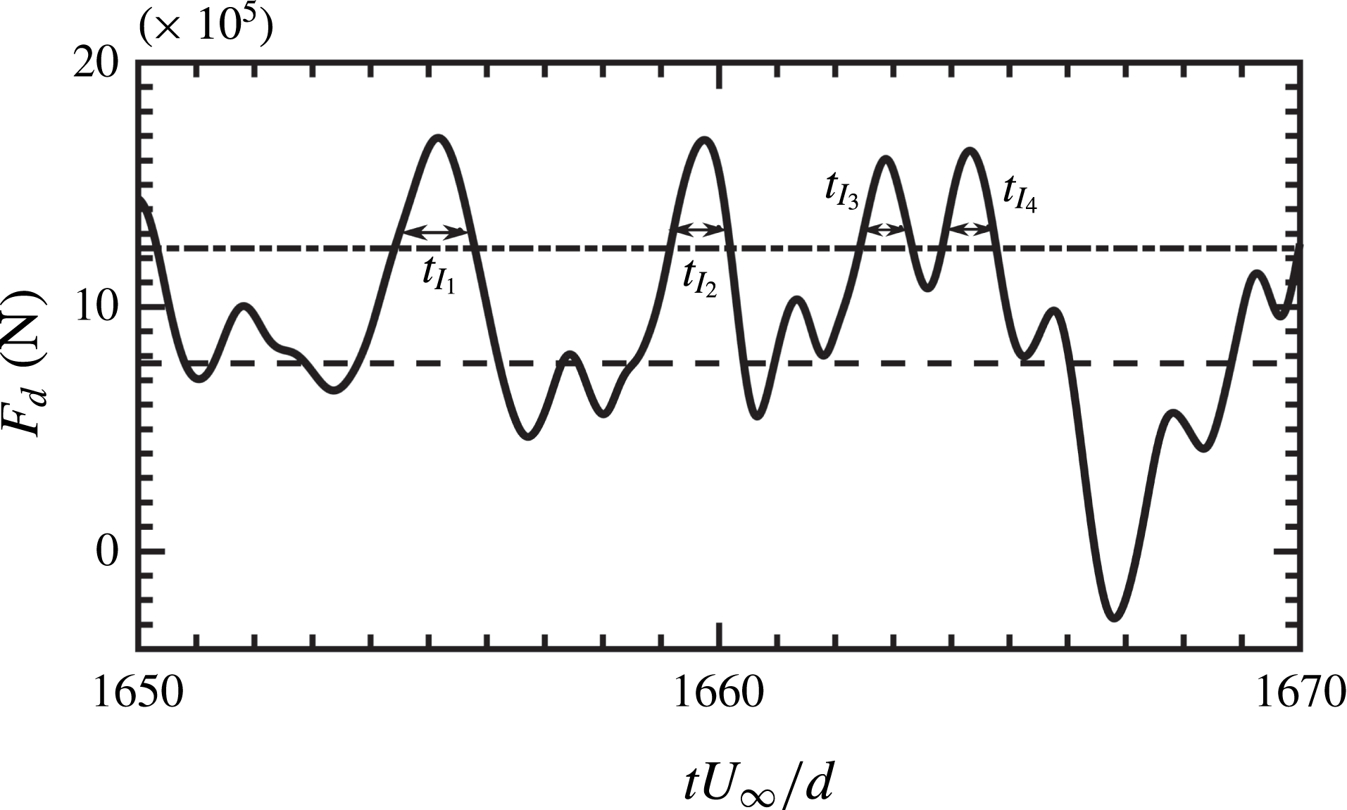
Consider a sample time history of the drag force (
 $F_{D}$
) on a large-diameter particle as shown in figure 15. In this case, although the period-averaged drag force (dashed line) on the particle is less than the specified threshold (dash-dotted line), an instantaneous force exceeding the threshold for a long duration could still possibly result in particle dislodgement (Diplas et al.
Reference Diplas, Dancey, Celik, Valyrakis, Greer and Akar2008). As shown in figure 15, such extreme force events are identified when the instantaneous force value exceeds the threshold and then the durations of such events (
 $t_{I_{1}}$
,
 $t_{I_{2}}$
,
 $t_{I_{3}}$
, etc.) are computed. Based on this, the impulse on a particle for a given duration is calculated using
 $$\begin{eqnarray}\displaystyle & \displaystyle \text{impulse}=I(\unicode[STIX]{x1D719}>\unicode[STIX]{x1D719}_{thr})=\int _{t_{I}}\unicode[STIX]{x1D719}\,\text{d}t, & \displaystyle\end{eqnarray}$$
where
 $\unicode[STIX]{x1D719}_{thr}$
is the specified threshold value of the variable
 $\unicode[STIX]{x1D719}$
. Implementing this procedure for the LP and SP cases, the number of such peak force events, their duration and impulse magnitude are calculated for various threshold conditions (
 $0\leqslant \unicode[STIX]{x1D719}_{thr}/\unicode[STIX]{x1D70E}_{\unicode[STIX]{x1D719}}\leqslant 5$
). Subsequently, averaging is carried out for number of particles and flow cycles. Note that change in the sign of the drag force after flow reversal is taken into consideration while identifying peak force events.
Representative time history (——) of the drag force (
 $F_{D}$
) in the LP case. Period-averaged drag force (- - - -) along with the specified threshold,
 $\unicode[STIX]{x1D719}_{thr}/\unicode[STIX]{x1D70E}_{\unicode[STIX]{x1D719}}=1$
(— ⋅ —) are also indicated. Local peaks in
 $F_{D}$
exceeding the threshold are detected as shown. The widths of the local peaks indicate their duration
 $t_{I}$
.

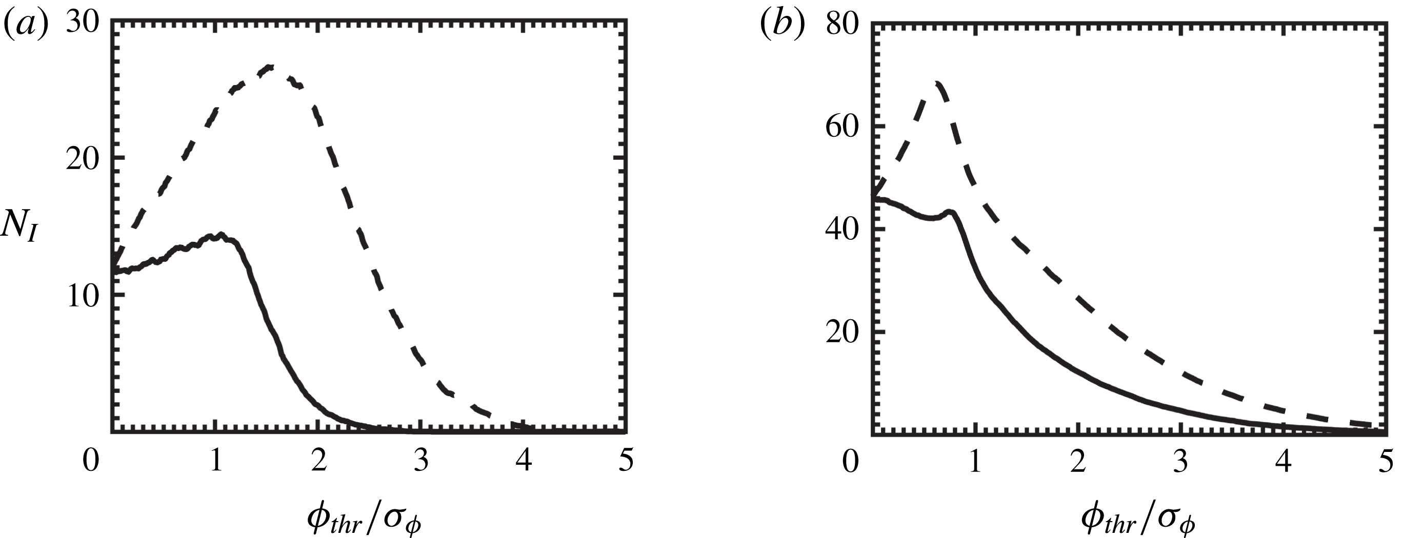
Variation with threshold values for (a) LP and (b) SP, of average number of peak force events,
 $N_{I}$
, experienced by a particle per flow cycle. The lines indicate drag (——) and lift (- - - -).

Figures 16(a) and 16(b) show average number of intervals,
 $N_{I}$
, of peak force events per flow cycle for the LP and SP cases, respectively. In both flow cases, the number of intervals for the lift force is typically larger than that for the drag force, indicating higher intermittency in the lift. In the case of LP, the number of intervals
 $N_{I}$
initially increases (more rapidly for the lift) with increase in the threshold, indicating the presence of relatively low-magnitude and high-frequency local peaks. Note that these local peaks are otherwise counted as a single peak for small threshold values under the present peak detection scheme as represented in figure 15. With further increase in the threshold value,
 $N_{I}$
for drag and lift begins to decline gradually isolating extreme force events. As shown in figure 16(a), peak value
 $N_{I}$
for the lift is almost twice as high as that for the drag. Therefore, in comparison to the drag, the number of high-frequency peak events is typically more in the case of lift. Moreover, the peak in the magnitude of
 $N_{I}$
for drag (lift) is seen at
 $\unicode[STIX]{x1D719}_{thr}/\unicode[STIX]{x1D70E}_{\unicode[STIX]{x1D719}}\approx 1~(2)$
. This further shows that, on average, extreme events in the lift force for the large-diameter particle also have higher magnitudes compared to those in the drag.
In the case of SP, this behaviour is more intricate. Consistent with the LP case,
 $N_{I}$
for the lift in the SP case initially increases rapidly with increase in the threshold, indicating the presence of low-magnitude local peaks; however,
 $N_{I}$
for the drag decreases slowly, exhibiting a local maximum close to
 $\unicode[STIX]{x1D719}_{thr}/\unicode[STIX]{x1D70E}_{\unicode[STIX]{x1D719}}\approx 0.6$
. Based on figure 16(b), two observations for the SP case can be drawn, as follows. First, similar to the LP case, the peak in the
 $N_{I}$
for the lift is almost 1.5–2 times higher than that for the drag. And second, both the peaks are observed at around the same threshold value (
 $\unicode[STIX]{x1D719}_{thr}/\unicode[STIX]{x1D70E}_{\unicode[STIX]{x1D719}}\approx 0.6$
). The former suggests that the lift data consist of more high-frequency peak events than those found in the drag, whereas the latter indicates that the peaks in the lift and drag force have comparable magnitudes.
Furthermore, all the profiles for
 $N_{I}$
in both LP and SP cases exhibit a recognizable change in the slope after which the drop in the value of
 $N_{I}$
is more gradual (e.g. after
 $\unicode[STIX]{x1D719}_{thr}/\unicode[STIX]{x1D70E}_{\unicode[STIX]{x1D719}}\approx 1$
in the SP case). Such flattening of profiles can be interpreted as the presence of well-pronounced isolated peaks in the drag and lift forces that keep getting detected even with the increase in the threshold value.
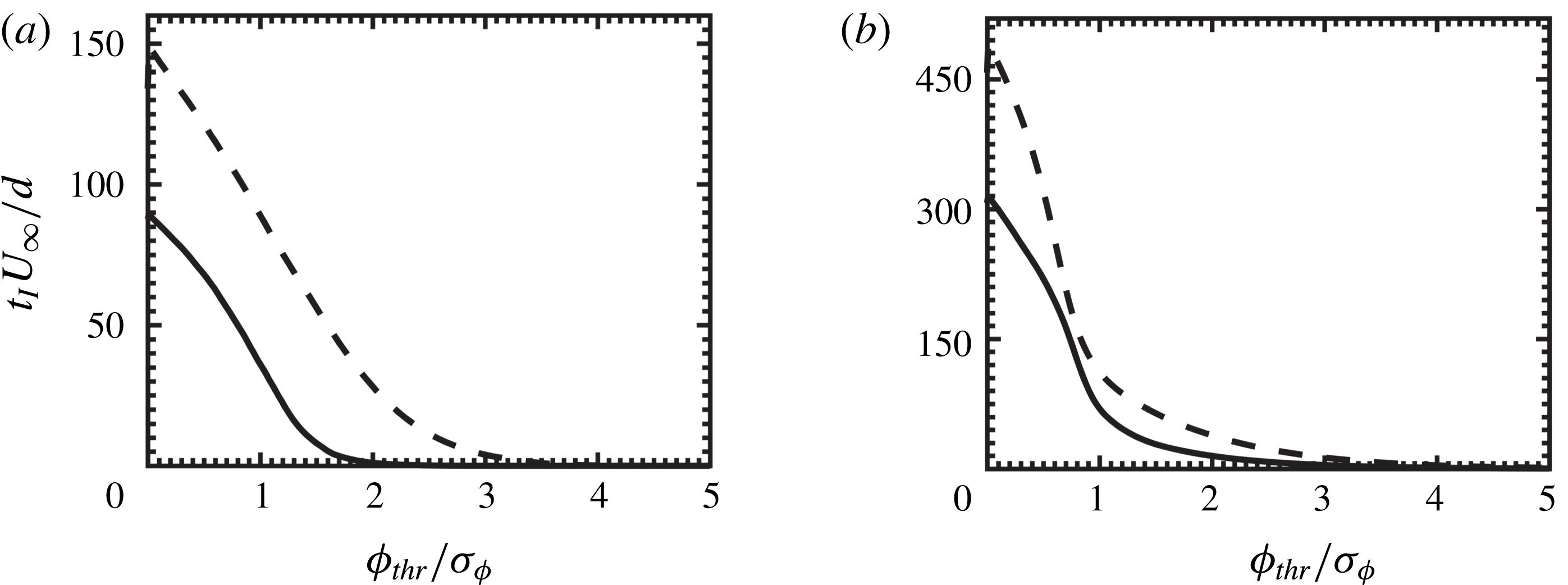
Figures 17(a) and 17(b) respectively show variation of average duration,
 $t_{I}$
, of peak force events per flow cycle for the LP and SP cases. In the case of LP, the time duration of lift is typically 1.5–2 times longer than that of the drag force. This corroborates figure 16(a,b), suggesting the presence of more high-frequency peak events in the lift that results in larger time duration compared to drag, albeit, for the small-diameter particle, this difference in drag and lift duration is indeed smaller. In both LP and SP cases, average time duration decreases with increase in the threshold value. Also, as shown in figure 17(a,b), there exists a sudden change in the slope of the profiles. As the threshold value increases, it is evident that the change in
 $t_{I}$
is more gradual. This is in accordance with figure 16(a,b) and further provides the evidence for the presence of pronounced isolated peaks in drag and lift forces.
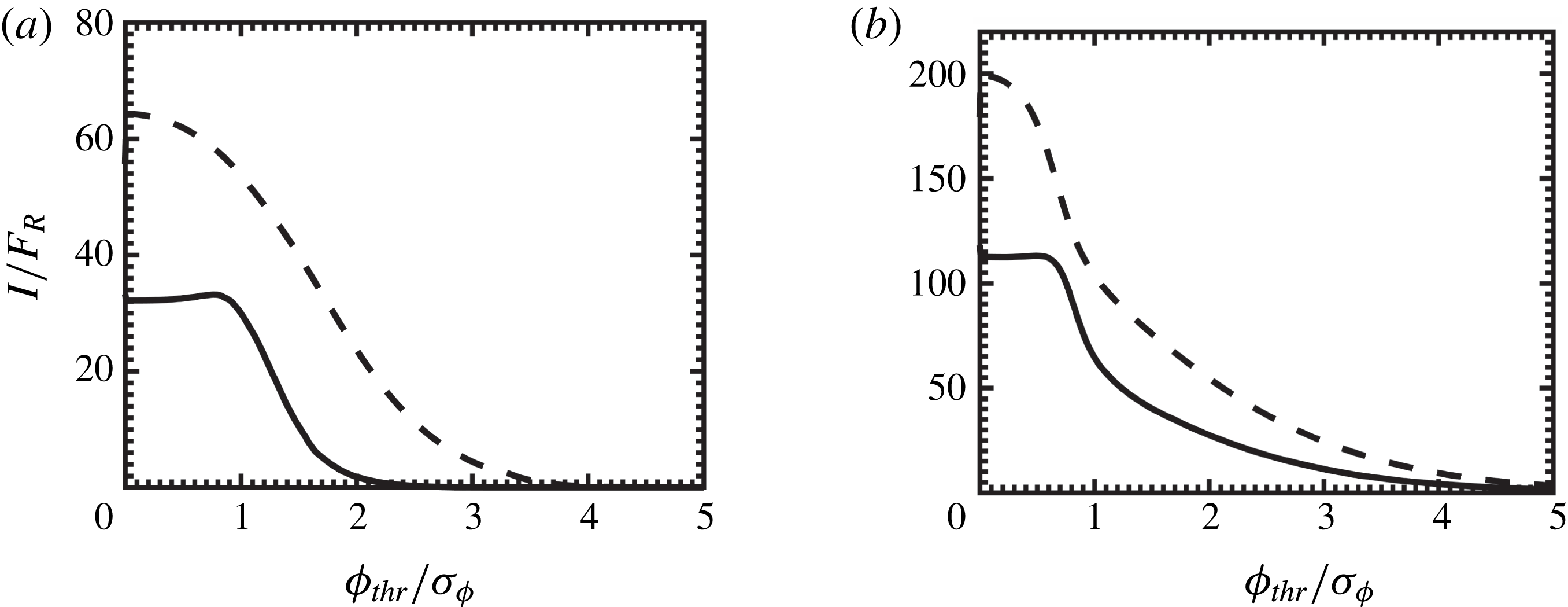
Based on this, an average impulse on a particle per flow cycle is calculated using (3.4) and is plotted in figures 18(a) and 18(b) for the LP and SP cases, respectively. Consistent with the earlier observations, the impulse based on the lift force is higher than that based on the drag. With increase in the threshold, the impulse related to the lift for LP (SP) particle is seen to decrease; however, that of the drag almost stays constant up to the threshold value of 1 (0.7). It is possible that the impulse based on the drag is dominated by a few local events that get detected until this threshold value. Again, the profiles of average impulse show very gradual decrease for high threshold values. For the purpose of illustration, the distribution of impulse events at a threshold value
 $\unicode[STIX]{x1D719}_{thr}/\unicode[STIX]{x1D70E}_{\unicode[STIX]{x1D719}}=1$
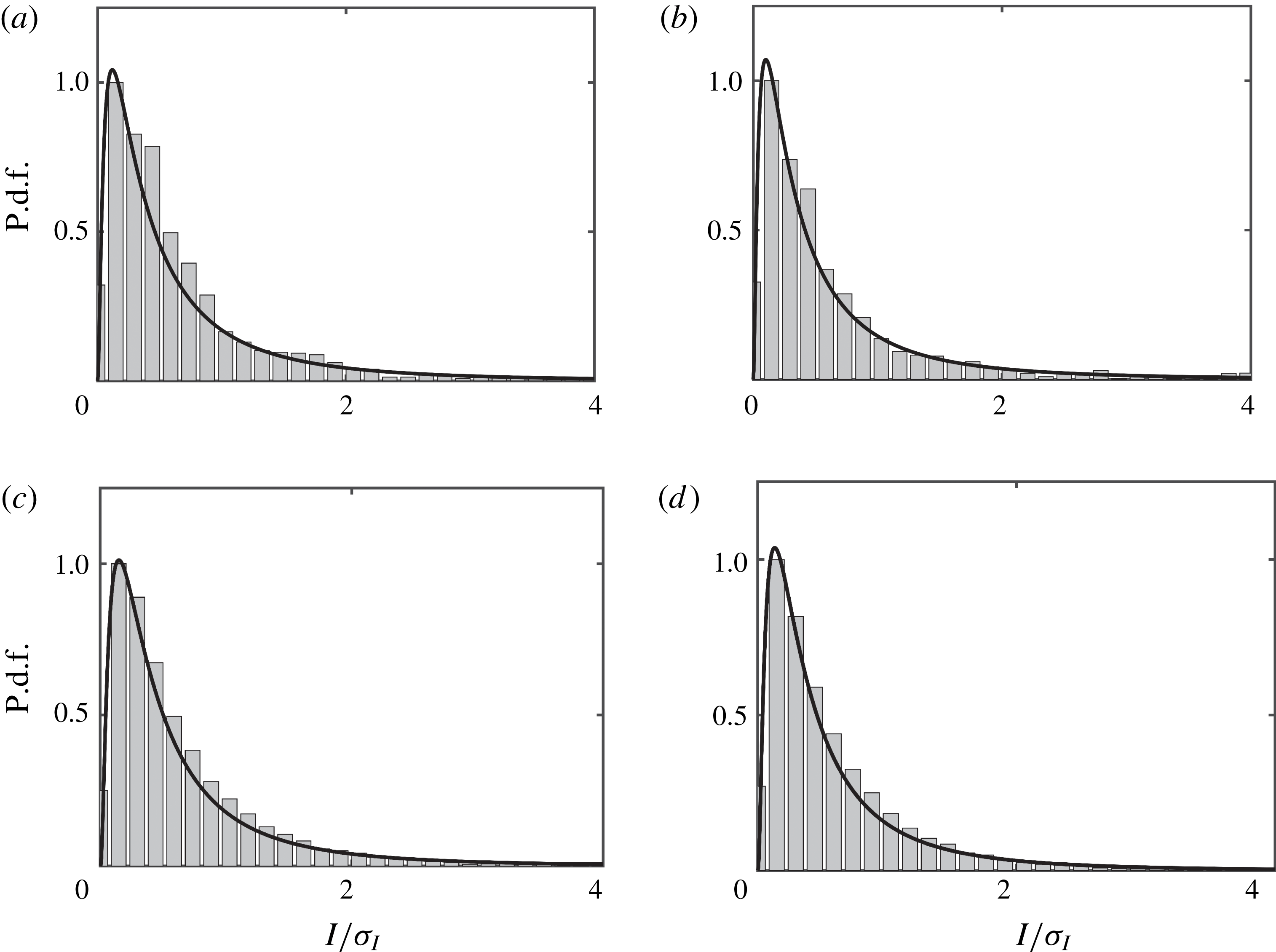
is plotted in figure 19 for (a) LP and (b) SP case. All distributions are heavily and positively skewed and are well described by a generalized extreme value distribution.
Variation with threshold values of average time duration of peak force events,
 $t_{I}U_{\infty }/d$
, for a particle per flow cycle. Line styles and panels are the same as in figure 16.

Variation with threshold values of average impulse,
 $I$
, for a particle per flow cycle. Here,
 $F_{R}=\unicode[STIX]{x1D70C}u_{\unicode[STIX]{x1D70F},max}^{2}A_{s}U_{\infty }/d$
, where
 $A_{s}$
is the projected area of a single spherical particle given by
 $\unicode[STIX]{x03C0}d^{2}/4$
. Line styles and panels are the same as in figure 16.

Distribution of impulse normalized by standard deviations at a threshold
 $\unicode[STIX]{x1D719}_{thr}/\unicode[STIX]{x1D70E}_{\unicode[STIX]{x1D719}}=1$
for (a,c) drag force and (b,d) lift force represented by histograms. Panels (a,b) and (c,d) are for the LP and SP cases, respectively.

Based on these results, it is reasonable to suggest that using a threshold value
 $\unicode[STIX]{x1D719}_{thr}/\unicode[STIX]{x1D70E}_{\unicode[STIX]{x1D719}}>1.5$
(2) for drag and lift in the case of LP (SP) might be sufficient to identify well-pronounced peak events. As noted earlier, the present study considers a roughness bed made up of fixed particles and therefore it is only conjectured that these events could possibly result in particle dislodgement, a subject of future investigation. Nevertheless, these results are typically in agreement with recently reported unidirectional studies (Chan-Braun Reference Chan-Braun2012; Celik et al.
Reference Celik, Diplas and Dancey2014). For example, Celik et al. (Reference Celik, Diplas and Dancey2014) used a threshold value based on the pressure,
 $\unicode[STIX]{x1D719}_{thr}/\unicode[STIX]{x1D70E}_{\unicode[STIX]{x1D719}}=2$
for
 $D^{+}$
values between 330 and 440. The distribution of impulse events reported by Celik et al. (Reference Celik, Diplas, Dancey and Valyrakis2010, Reference Celik, Diplas and Dancey2013, Reference Celik, Diplas and Dancey2014) also showed highly skewed nature similar to that observed in figure 19.
3.9 Summarizing implications of flow oscillations
The oscillatory nature of the near-bed turbulence governs the overall structure of hydrodynamic forces on the particle bed. As expected in the case of wall-bounded oscillatory flows, the near-bed flow depending on the Reynolds number is typically out of sync with the external pressure gradient, resulting in early deceleration of local flow in the vicinity of the particle bed. As a consequence of this, the drag and lift record shows a phase delay with the free-stream velocity. Furthermore, contrary to unidirectional flows, turbulence is present only in some part of the oscillation cycle. In the present investigation, especially for the small-diameter particle case, the sudden occurrence of turbulence followed by flow relaminarization is evident; the former provides favourable conditions for dislodgement of the particles, whereas the latter typically offers stability to the particle bed. Such behaviour of near-bed flow also greatly influences the spatial structure of the forces on the particles, resulting in local patches of positive/negative forces. As a result, strong non-Gaussian behaviour of both fluctuating near-bed flow and force statistics is observed in oscillatory flows.
On the other hand, although the overall structure of turbulent oscillatory flow differs significantly from that of unidirectional flow, there are some similarities in the characteristics of drag/lift forces that appear to be robust. For example, cross-correlation of drag and lift depicts qualitatively similar variation as that observed in other unidirectional studies, albeit with differences in the amplitudes of maxima and minima. In addition, scaling regions observed in force spectra as well as the distribution of impulse events suggest the universal nature of force fluctuations on the particle bed.
3.10 Implications for the sediment incipient motion models
In the present investigation, a rough bed made up of a single layer of hexagonally packed fixed spherical particles is considered. Although using such an idealized flow set-up may limit the scope of application of the present results to specific problems, it still provides us with a detailed understanding of particle–turbulence interactions, which are in turn responsible for sediment incipient motion. The novelty of the present investigation is to provide data, without requiring any ad hoc models, on the temporal variations in the magnitude of drag and lift forces on the sediment bed, the time scales associated with these variations, and their correlations with near-bed turbulence in an oscillatory flow environment. The three-dimensional correlation function between particle forces and near-bed turbulent flow reveals the presence of a significant correlation region, the shape of which remained unchanged between large- and small-diameter particle cases. Velocity and pressure fluctuations measured in such high-correlation regions follow a fourth-order Gram–Charlier distribution, and it is demonstrated that the distribution of hydrodynamic forces on the particle bed could be constructed using such higher-order flow statistics. In other words, it is possible to obtain the particle force distribution by simply measuring the velocity or pressure fluctuations in such high-correlation regions. In this section, a brief summary giving a few examples of how such detailed flow information could be used in developing sediment erosion models is presented.
Computations of sediment-laden flows typically employ simplistic models to study sediment transport, in particular, onset of sediment erosion (Bagnold Reference Bagnold1966; Fredsøe & Deigaard Reference Fredsøe and Deigaard1992; Nelson et al.
Reference Nelson, Schmeeckle, Shreve and McLean2000; Nino et al.
Reference Nino, Lopez and Garcia2003). Historically, these models are based on the Shields parameter,
 $\unicode[STIX]{x1D703}=\bar{\unicode[STIX]{x1D70F}}_{w}/(\unicode[STIX]{x1D70C}_{p}-\unicode[STIX]{x1D70C})gd$
(Shields Reference Shields1936), which is the ratio of average bed shear stress (
 $\bar{\unicode[STIX]{x1D70F}}_{w}$
) to the stabilizing settling force due to gravitational acceleration (
 $g$
). Here,
 $\unicode[STIX]{x1D70C}_{p}$
and
 $\unicode[STIX]{x1D70C}$
are sediment and fluid densities, respectively, and
 $d$
is the average particle size. Based on this, rates of sediment pickup (
 $P_{k}$
) could be expressed with a relationship,
 $P_{k}\propto (\unicode[STIX]{x1D703}-\unicode[STIX]{x1D703}_{c})$
. For example, the sediment pickup rate reported by Van Rijn (Reference Van Rijn1984) has been widely used in many sediment erosion studies and is given by
 $$\begin{eqnarray}\displaystyle & \displaystyle \frac{P_{k}}{\sqrt{\displaystyle \frac{(\unicode[STIX]{x1D70C}_{p}-\unicode[STIX]{x1D70C})}{\unicode[STIX]{x1D70C}}gd}}=\unicode[STIX]{x1D6FC}\left(\frac{\unicode[STIX]{x1D703}-\unicode[STIX]{x1D703}_{c}}{\unicode[STIX]{x1D703}_{c}}\right)^{\unicode[STIX]{x1D6FE}}\left(\frac{(\unicode[STIX]{x1D70C}_{p}-\unicode[STIX]{x1D70C})gd^{3}}{\unicode[STIX]{x1D70C}\unicode[STIX]{x1D708}^{2}}\right)^{\unicode[STIX]{x1D6FD}}, & \displaystyle\end{eqnarray}$$
where
 $\unicode[STIX]{x1D703}_{c}$
is the critical Shields parameter, and constants
 $\unicode[STIX]{x1D6FC}$
,
 $\unicode[STIX]{x1D6FD}$
and
 $\unicode[STIX]{x1D6FE}$
are obtained using a fit to experimental data. Assuming the erosion is initiated by lift forces alone, a simple force balance between hydrodynamic lift force and the buoyant weight of the particle yields an expression for the critical Shields parameter and is given as (Chan-Braun et al.
Reference Chan-Braun, Garcia-Villalba and Uhlmann2011)
 $$\begin{eqnarray}\displaystyle & \displaystyle \unicode[STIX]{x1D703}_{c}=\frac{2}{3\widehat{C}_{L}}, & \displaystyle\end{eqnarray}$$
where
 $\widehat{C}_{L}$
is the lift coefficient with a slightly different normalization and is defined as
 $\widehat{C}_{L}=F_{L}/(\unicode[STIX]{x1D70C}u_{\unicode[STIX]{x1D70F}}^{2}d^{2}\unicode[STIX]{x03C0}/4)$
. Calculation of
 $\unicode[STIX]{x1D703}_{c}$
therefore requires information of force statistics. Most of the erosion models typically assume a constant value for the lift coefficient. However, the present DNS investigation reveals a large intermittency in the lift forces, resulting in longer tails of force distributions. Such DNS investigation is therefore useful in providing accurate descriptions of force statistics to calculate instantaneous critical values of the Shields parameter. In addition, most of these models are deterministically based on mean values of the bed shear stress, and do not consider particle size, shape, bed arrangements, or multi-scale interactions between turbulent flow and sediment particles. Using DNS results, such as these, however, it is possible to incorporate the effects of particle–turbulence interactions and provide time-dependent wall shear stress information to calculate the instantaneous pickup rate,
 $P_{k}(t)$
, of sediment grains. For example, it is possible to include higher-order flow statistics to calculate
 $\unicode[STIX]{x1D703}_{c}$
and lift coefficients. By doing so, it would then be possible to incorporate effects of fluctuations, in addition to mean stress, into an erosion criterion.
On the other hand, stochastic models of incipient motion, based on modelling the probability of particle entrainment, hold promise in accounting for the intermittent dynamics of turbulent flows (Einstein Reference Einstein1950; Mingmin & Qiwei Reference Mingmin and Qiwei1982; Cheng & Chiew Reference Cheng and Chiew1998; Papanicolaou et al.
Reference Papanicolaou, Diplas, Evaggelopoulos and Fotopoulos2002; Wu & Lin Reference Wu and Lin2002; Cheng & Law Reference Cheng and Law2003; Wu & Chou Reference Wu and Chou2003; Wu & Kuo-Hsin Reference Wu and Kuo-Hsin2004; Hofland & Battjes Reference Hofland and Battjes2006). Such models often depend on many factors, including particle force statistics, instantaneous bed shear stress, near-bed flow statistics, critical impulse, among others. For example, the probability of particle entrainment (
 $P_{E}$
) can be determined by integrating p.d.f.s of lift, drag or shear stress acting on the particle bed over the range of forces that would result in particle dislodgement and is given as
 $$\begin{eqnarray}\displaystyle & \displaystyle P_{E}=1-\int _{-F_{cr}}^{F_{cr}}f(F)\,\text{d}F, & \displaystyle\end{eqnarray}$$
where
 $F$
is the force in question (e.g. lift) and
 $F_{cr}$
is the critical value of the force at which sediment motion occurs (Papanicolaou et al.
Reference Papanicolaou, Diplas, Evaggelopoulos and Fotopoulos2002; Wu & Kuo-Hsin Reference Wu and Kuo-Hsin2004). Calculation of
 $F$
and
 $F_{cr}$
requires information about near-bed velocity (
 $u_{b}$
) and force coefficients such as
 $C_{D}$
or
 $C_{L}$
. For a well-packed particle bed, such as the present one, movement of the particle typically occurs if the lift force exceeds the submerged weight of the particle (Papanicolaou et al.
Reference Papanicolaou, Diplas, Evaggelopoulos and Fotopoulos2002). In such cases, the pickup probability of lifting can be defined as (Wu & Lin Reference Wu and Lin2002)
 $$\begin{eqnarray}\displaystyle & \displaystyle P_{L}=P(F_{L}>W)=P(u_{b}^{2}>B_{L}^{2})=P(u_{b}>B_{L})+P(u_{b}<-B_{L}), & \displaystyle\end{eqnarray}$$
where
 $F_{L}=C_{L}(\unicode[STIX]{x03C0}d^{2}/4)(\unicode[STIX]{x1D70C}u_{b}^{2}/2)$
is the instantaneous lift force,
 $W=(\unicode[STIX]{x1D70C}_{p}-\unicode[STIX]{x1D70C})g(\unicode[STIX]{x03C0}d^{3}/6)$
is the submerged weight of the particle and
 $B_{L}=(4(\unicode[STIX]{x1D70C}_{p}-\unicode[STIX]{x1D70C})gd/3\unicode[STIX]{x1D70C}C_{L})^{0.5}$
denotes the lifting threshold. Based on this, the probability of entrainment in the lifting mode can be calculated as
 $$\begin{eqnarray}\displaystyle & \displaystyle P_{L}=1-\int _{-B_{L}}^{B_{L}}f(u_{b})\,\text{d}u_{b}. & \displaystyle\end{eqnarray}$$
Calculation of such a probability therefore often requires knowledge of the near-bed velocity distribution along with force statistics. Most of the present models typically assume Gaussian or log-normal distribution for near-bed velocity fluctuations (Papanicolaou et al.
Reference Papanicolaou, Diplas, Evaggelopoulos and Fotopoulos2002; Wu & Lin Reference Wu and Lin2002; Cheng & Law Reference Cheng and Law2003; Wu & Chou Reference Wu and Chou2003). Also, as mentioned earlier, computations or measurements of time-varying drag and lift force coefficients are not straightforward. Instead, in many instances, they are assumed to be constant. The present DNS study provides many details, including an accurate description of near-bed flow that follows a fourth-order Gram–Charlier distribution along with time-accurate force statistics. Using such information in stochastic models would therefore facilitate incorporation of higher-order turbulent flow statistics to account for the effects of particle–turbulence interactions, flow oscillations along with near-bed turbulent bursting phenomenon. These results also verify the validity of the fourth-order Gram–Charlier based theoretical model reported by Wu & Kuo-Hsin (Reference Wu and Kuo-Hsin2004). In addition, Diplas et al. (Reference Diplas, Dancey, Celik, Valyrakis, Greer and Akar2008), Celik et al. (Reference Celik, Diplas, Dancey and Valyrakis2010) and Valyrakis et al. (Reference Valyrakis, Diplas, Dancey, Greer and Celik2010) demonstrated the suitability of the impulse concept, providing an additional degree of freedom, time, to predict the particle dislodgement under turbulent flow conditions. In accordance with earlier theoretical studies (Celik et al.
Reference Celik, Diplas, Dancey and Valyrakis2010; Valyrakis et al.
Reference Valyrakis, Diplas, Dancey, Greer and Celik2010), the present DNS results also show impulse events to be positively skewed and to follow a generalized extreme value distribution; results that could be used to find the probability of particle entrainment as reported by Celik et al. (Reference Celik, Diplas, Dancey and Valyrakis2010). Also, characterization of impulse-generating force events suggests that a threshold value of
 $\unicode[STIX]{x1D719}_{thr}/\unicode[STIX]{x1D70E}_{\unicode[STIX]{x1D719}}\approx 2$
might be sufficient to identify well-pronounced peak events that could play an important role in dislodging the particle. These results are in agreement with recently reported unidirectional studies (Chan-Braun Reference Chan-Braun2012; Celik et al.
Reference Celik, Diplas and Dancey2014).
Studying high-Reynolds-number flows, the majority of sediment transport calculations often employ a large-eddy simulation (LES) approach. Such LES calculations of sediment erosion with an Eulerian two-fluid type model typically require a boundary condition for the flux of the sediment and is given by
 $$\begin{eqnarray}\displaystyle & \displaystyle \frac{\unicode[STIX]{x1D708}_{T}}{Pr_{T}}\frac{\unicode[STIX]{x2202}\overline{C}}{\unicode[STIX]{x2202}z}=-P_{k}, & \displaystyle\end{eqnarray}$$
where
 $\unicode[STIX]{x1D708}_{T}$
is the eddy viscosity,
 $Pr_{T}$
is the turbulent Prandtl number,
 $\overline{C}$
is the grid-filtered sediment concentration and
 $z$
represents the wall-normal direction. Using time-accurate flow information from DNS investigation, it is possible to specify turbulent flow properties along with an instantaneous sediment pickup rate that is also non-uniform and varies spatially,
 $P_{k}(t,x,y)$
.
The present DNS data could therefore be useful in many such ways to provide inputs to existing sediment erosion models. Such detailed information would possibly allow us to devise a refined erosion criterion for oscillatory flows. In order to study actual erosion events, however, a DNS investigation with moving particles is needed and is a subject of future investigation.
4 Summary
The present investigation focused on studying the spatial and temporal structure of unsteady hydrodynamic forces on a particle bed subjected to an oscillatory flow environment. Two particle sizes of diameter 372 and 125 in wall units in a very rough turbulent flow regime are studied. Characterization of unsteady drag and lift forces in terms of spatial distribution, temporal autocorrelation, force spectrum as well as cross-correlations with measurable flow variables were carried out. The implications of selecting a certain threshold criterion for erosion onset based on the intermittency in the unsteady forces were also reported.
The time history of phase-averaged drag and lift force showed discernible differences between large- and small-diameter particle cases. In the case of large particle, both drag and lift coefficients peak earlier in the flow cycle, exhibiting phase lag with the free-stream velocity. Conversely, as a result of increased Reynolds number
 $Re_{a}$
, this phase lag is considerably reduced in the case of small-diameter particles. The small phase lag between drag and lift typically observed for the larger particles was also seen to decrease in the case of smaller particles. Moreover, the presence of sharp spikes in drag and lift records was detected for the small-diameter particle but was absent in the large-diameter case. Such distinct spikes were attributed to the sudden occurrence of turbulence close to the peak phase in the smaller-particle case.
In both flow cases, the period-averaged lift and drag coefficients remained positive. Higher-order moments such as skewness and kurtosis of drag and lift fluctuations were found to exhibit strong non-Gaussian behaviour. For both flow cases, skewness values of drag and lift fluctuations were positive. High values of kurtosis indicated large intermittency in the forces that resulted in longer tails of rare but strong events. Also, kurtosis values in the small-particle case were almost twice as large as in the large-particle case, indicating the larger intermittency in the forces for the former case.
The spatial distribution of the forces revealed a region of strong positive drag component of the stress near the top of the sphere, along with small patches of weak positive drag-related stress in the front and the aft portion of the particle; the latter was only present in the case of the large-diameter particle bed. Lift-related stress of positive magnitude was observed mostly in the top portion of the upper hemisphere of the small particle, a result of lower values of pressure due to flow acceleration near the particle crest. In the case of a large particle, positive lift-related stress was mostly distributed on the side and the aft region of the particle. This was found to be the effect of enhanced three-dimensionality of the boundary layer and shielding effects along with the complex pore-scale flow in the gaps between the particles, all typically more pronounced in the case of large-diameter particles.
The time scales of drag and lift fluctuations were studied by means of temporal autocorrelation functions. The broken near-bed structures of a size comparable to the large particle resulting from flow isotropization governed the time scales of fluctuating forces on the large-particle bed. As a result, the integral and Taylor micro-scales of drag and lift fluctuations on the large particle were of the order of unity. Conversely, larger separation of scales causing disparity in integral and Taylor micro-scales was observed in the case of small-diameter particles; the former was typically 4–8 times larger than latter, and was argued to be a result of elongated near-bed structures found in the small-particle case.
Cross-correlations between drag and lift were also studied. In both flow cases, drag and lift, on average, were positively correlated with a time delay, which was approximately equal to the Taylor micro-scale related to drag/lift fluctuations. Such behaviour of the cross-correlation function appears to be very robust, as it is in general agreement with previously reported experimental studies that dealt with different flow conditions, particle Reynolds number, particle shape and arrangement, etc.
The spectral content of drag and lift fluctuations was examined by plotting their frequency spectra. In both flow cases, a reasonably good collapse of spectra for drag and lift fluctuations was observed, with the largest spectral contributions at lower frequencies. Two scaling regions,
 $-11/3$
and
 $-7/3$
in the mid- and high-frequency regions, respectively, were observed for all the spectra; the former typically represents turbulence–mean-shear interactions, whereas the latter indicates the dominance of turbulence–turbulence interactions. In comparison to the large-particle case,
 $-11/3$
scaling region for the smaller particles was present up to higher frequencies, suggesting that a wider range of scales was dominated by turbulence–mean-shear interactions. Again, the present data for both cases exhibit similar behaviour as that observed in previously reported unidirectional studies, and therefore indicates the universal nature of the force fluctuations on the roughness bed.
The three-dimensional cross-correlation function between drag (lift) and velocity (pressure) revealed the direct link between flow parameters and force fluctuations. The drag force was well correlated with the streamwise velocity fluctuations upstream and downstream of the particle centre in the streamwise direction, along with the wing-shaped positive correlation in the spanwise direction for both flow cases. In comparison to the large-diameter particle case, the spatial extent of drag–velocity correlation was 2–3 times larger in homogeneous directions for the small particles, a feature that is reminiscent of longer near-bed structures typically found in the case of the small-diameter particle bed. In both flow cases, the pressure fluctuations were anti-correlated with the lift force in the regions around the particle when plotted in the zero spanwise shift plane. The wing-shaped positive correlation in the spanwise direction was also observed for lift–pressure fluctuations. In addition, p.d.f. distributions of drag (lift) fluctuations, in particular, peakedness and long tails, matched remarkably well with fourth-order Gram–Charlier distributions of velocity (pressure) fluctuations.
Finally, characterization of impulse-generating force events was carried out by studying the number and average duration of such events. In both flow cases, higher intermittency was found in the lift force compared to the drag. The magnitude of the impulse showed a gradual decrease for large threshold values, indicating the presence of isolated well-pronounced peaks in the particle-bed forces. The distributions of impulse events for both flow cases were heavily and positively skewed and were well described by a generalized extreme value distribution. Such statistical analysis of force intermittency is especially critical for better specification of a threshold value in erosion models.
Acknowledgements
This work was supported by the National Science Foundation (NSF-CBET, 1133363). The computations were performed on the TACC-Stampede machine. The authors thank Dr J. Urzay of Stanford University for fruitful discussions during the CTR Summer Program 2014. The authors appreciate the valuable suggestions from Dr B. Vowinckel. They also thank the anonymous reviewers for their useful suggestions leading to the improvement of the manuscript.
Appendix A. Computational approach
In this work, a simple uniform Cartesian and non-conforming (to any immersed boundaries) grid is used for flow predictions. The fictitious-domain method is used in this study to simulate the flow through a randomly packed bed; a detailed description of this method is available in the works of Apte and co-workers (Apte, Martin & Patankar Reference Apte, Martin and Patankar2009c ; Apte & Finn Reference Apte and Finn2013). Description of the mathematical formulation of the method, and the generation of the immersed-boundary objects is briefly summarized below.
A.1 Mathematical formulation
Let
 $\unicode[STIX]{x1D6E4}$
be the computational domain, which includes both the fluid (
 $\unicode[STIX]{x1D6E4}_{F}(t)$
) and the particle (
 $\unicode[STIX]{x1D6E4}_{P}(t)$
) domains. A structured Cartesian grid is generated throughout the fluid as well as particle domains. Let the fluid boundary not shared with the particle be denoted by
 ${\mathcal{B}}$
and have a Dirichlet condition (generalization of boundary conditions is possible). The basis of the fictitious-domain-based approach (Glowinski et al.
Reference Glowinski, Pan, Hesla, Joseph and Periaux2001) is to extend the Navier–Stokes equations for fluid motion over the entire domain
 $\unicode[STIX]{x1D6E4}$
inclusive of particle regions. The natural choice is to assume that the particle region is filled with a Newtonian fluid. Both the fluid and the particle regions will be assumed to be incompressible and thus the incompressibility constraint applies over the entire region. In addition, as the particles are assumed to be rigid, the motion of the material inside the particle is constrained to be a rigid-body motion.
The momentum equation for motion of the incompressible, constant-density and constant-viscosity fluid in the entire domain
 $\unicode[STIX]{x1D6E4}$
is given by
 $$\begin{eqnarray}\displaystyle & \displaystyle \unicode[STIX]{x1D735}\boldsymbol{\cdot }\boldsymbol{v}=0, & \displaystyle\end{eqnarray}$$
 $$\begin{eqnarray}\displaystyle & \displaystyle \unicode[STIX]{x1D70C}\left(\frac{\unicode[STIX]{x2202}\boldsymbol{v}}{\unicode[STIX]{x2202}t}+\left(\boldsymbol{v}\boldsymbol{\cdot }\unicode[STIX]{x1D735}\right)\boldsymbol{v}\right)=-\unicode[STIX]{x1D735}p+\unicode[STIX]{x1D707}\unicode[STIX]{x1D6FB}^{2}\boldsymbol{v}+\unicode[STIX]{x1D70C}\boldsymbol{g}+\boldsymbol{f}, & \displaystyle\end{eqnarray}$$
where
 $\boldsymbol{u}$
is the velocity vector (with components given by
 $\boldsymbol{v}=(v_{x},v_{y},v_{z})$
),
 $\unicode[STIX]{x1D70C}$
the density,
 $\unicode[STIX]{x1D707}$
the fluid viscosity,
 $p$
the pressure,
 $\boldsymbol{g}$
the gravitational acceleration, and
 $\boldsymbol{f}$
the additional body force, which is used to impose the rigid condition for the solid-phase part. A non-zero forcing function,
 $\boldsymbol{f}$
, is needed as a constraint to enforce the rigidity of the solid part. Inside the particle region, the rigid-body motion,
 $\boldsymbol{v}^{RBM}$
, implies a vanishing deformation-rate tensor (Apte & Finn Reference Apte and Finn2013)
 $$\begin{eqnarray}\displaystyle \displaystyle \left.\begin{array}{@{}c@{}}{\textstyle \frac{1}{2}}(\unicode[STIX]{x1D735}\boldsymbol{v}+(\unicode[STIX]{x1D735}\boldsymbol{v})^{\text{T}})=\unicode[STIX]{x1D63F}[\boldsymbol{v}]=0,\\[4.0pt] \Rightarrow \quad \boldsymbol{v}=\boldsymbol{v}^{RBM}=\boldsymbol{U}+\unicode[STIX]{x1D734}\times \boldsymbol{r},\end{array}\right\}~\text{in}~\unicode[STIX]{x1D6E4}_{P}. & & \displaystyle\end{eqnarray}$$
Here,
 $\boldsymbol{U}$
and
 $\unicode[STIX]{x1D734}$
are the translational and angular velocities of the object, and
 $\boldsymbol{r}$
is the position vector of a point inside the object from its centroid. For the fixed-bed problems considered here,
 $\boldsymbol{v}^{RBM}$
is always zero. The vanishing deformation-rate tensor for the rigidity constraint automatically ensures that the solid region is divergence-free and incompressible. The incompressibility constraint of divergence-free velocity field is enforced by solving a Laplace equation for the pressure field. Similarly, the tensor constraint
 $\unicode[STIX]{x1D63F}[\boldsymbol{v}]=0$
for rigid motion gives rise to a tensor field inside the solid region. Sharma & Patankar (Reference Sharma and Patankar2005) proposed an approach that provides the rigidity constraint explicitly, thus reducing the computational cost significantly. Note that the tensorial rigidity constraint can be reformulated to give
 $$\begin{eqnarray}\displaystyle \displaystyle \unicode[STIX]{x1D735}\boldsymbol{\cdot }(\unicode[STIX]{x1D63F}[\boldsymbol{v}]) & = & \displaystyle 0\quad \text{in}~\unicode[STIX]{x1D6E4}_{P},\end{eqnarray}$$
 $$\begin{eqnarray}\displaystyle \displaystyle \unicode[STIX]{x1D63F}[\boldsymbol{v}] & = & \displaystyle 0\quad \text{on solid}{-}\text{fluid interface},~\unicode[STIX]{x1D6FD}.\end{eqnarray}$$
A fractional-step algorithm can be devised to solve the fictitious-domain problem (Sharma & Patankar Reference Sharma and Patankar2005; Apte et al.
Reference Apte, Martin and Patankar2009c
; Apte & Finn Reference Apte and Finn2013). Knowing the solution at time level
 $t^{n}$
, the goal is to find
 $\boldsymbol{v}$
at time
 $t^{n+1}$
.
-
(1) In the first step, the rigidity constraint force
 $\boldsymbol{f}$
in (A 1) is set to zero and the equation together with the incompressibility constraint (A 3) is solved by standard fractional-step schemes over the entire domain. Accordingly, a pressure Poisson equation is derived and used to project the velocity field onto an incompressible solution. The obtained velocity field is denoted as
$\boldsymbol{v}^{n+1}$
inside the fluid domain and
$\hat{\boldsymbol{v}}$
inside the solid object.
-
(2) To solve for
$\boldsymbol{v}^{n+1}$
inside the solid region,
$\boldsymbol{f}$
is needed. The constraint on the deformation rate tensor given by (A 3), along with the no-slip specification at the solid–fluid interface, can be reformulated to obtain (A 6)
$$\begin{eqnarray}\displaystyle & \displaystyle \unicode[STIX]{x1D735}\boldsymbol{\cdot }(\unicode[STIX]{x1D63F}[\boldsymbol{v}^{n+1}])=\unicode[STIX]{x1D735}\boldsymbol{\cdot }\left(\unicode[STIX]{x1D63F}\left[\hat{\boldsymbol{v}}+\frac{\boldsymbol{f}\unicode[STIX]{x0394}t}{\unicode[STIX]{x1D70C}}\right]\right)=0, & \displaystyle\end{eqnarray}$$
(A 7)The velocity field in the solid is zero for fixed beads. Thus
$$\begin{eqnarray}\displaystyle & \displaystyle \unicode[STIX]{x1D63F}[\boldsymbol{v}^{n+1}]\boldsymbol{\cdot }\boldsymbol{n}=\unicode[STIX]{x1D63F}\left[\hat{\boldsymbol{v}}+\frac{\boldsymbol{f}\unicode[STIX]{x0394}t}{\unicode[STIX]{x1D70C}}\right]\boldsymbol{\cdot }\boldsymbol{n}=0. & \displaystyle\end{eqnarray}$$
$\hat{\boldsymbol{v}}$
is split into a rigid-body motion (
$\boldsymbol{v}^{RBM}=\boldsymbol{v}+\unicode[STIX]{x1D734}\times \boldsymbol{r}=0$
) and residual non-rigid motion (
$\boldsymbol{v}^{\prime }$
). The above formulation can be easily generalized to solid bodies with specified motion by directly setting
$\boldsymbol{v}^{RBM}$
to the specified velocity.
-
(3) The rigidity constraint force is then simply obtained as
$\boldsymbol{f}=\unicode[STIX]{x1D70C}(\boldsymbol{v}^{RBM}-\hat{\boldsymbol{v}})/\unicode[STIX]{x0394}t$
. This sets
$\boldsymbol{v}^{n+1}=\boldsymbol{v}^{RBM}$
in the solid domain. Note that the rigidity constraint is non-zero only inside the solid domain and zero everywhere else. This constraint is then imposed in a third fractional step.





The set of equations is computed for the whole domain, including the fluid and solid regions, by using the fictitious-domain approach. A fractional stepping algorithm together with an algebraic multigrid (AMG) solver for the pressure Poisson equation are implemented in a parallel three-dimensional version of the solver (Apte et al. Reference Apte, Martin and Patankar2009c ).
Schematic of material volumes within a circular object with sub-cell resolution.

A.2 Generation of immersed objects
To generate immersed objects and their interfaces on the background Cartesian grid, a triangulated representation of the surface and the associated outward normals to this representation are first generated. These were generated using CAD software. Marker points were defined on the surface; knowing the marker point and sphere centres, an outward normal was determined for each marker point. Representing multiple bead surfaces was straightforward using this approach.
Once the sphere surfaces were represented by marker points, the inside region of the particle is subdivided into cubic material volumes of size smaller than the background Cartesian mesh. This process helps to develop both a sharp representation of the boundary and an accurate representation of the rigidity constraint force. To illustrate the essential features of the process, an example of a circular interface with associated material volumes within the interface is provided in figure 20. The use of material volumes over the entire particle domain (as opposed to only around the particle surface) simplifies the calculation of the rigidity constraint force that is non-zero only inside the particle region. To preserve the accuracy of the scheme, consistent and conservative interpolations are necessary between the centres of the material volumes and the centres of the background Cartesian cells. Accordingly, interpolations that have compact support and typically used in immersed boundary method such as that developed by Roma, Peskin & Berger (Reference Roma, Peskin and Berger1999) are used.