


1 Introduction
This study is motivated by the desire to utilize active feedback controls to manipulate the inertially driven instabilities of a falling liquid film. Recently, Thompson et al. (Reference Thompson, Gomes, Pavliotis and Papageorgiou2016a ) showed that observations of the film surface shape combined with actuation applied by same-fluid blowing and suction through the rigid wall supporting the flow could be used to apply feedback control to a falling film, allowing stabilization of a wide range of states, including a uniform film, unstable travelling waves and even arbitrary states which would not be solutions of the original system. However, practical implementation of feedback via blowing and suction through the supporting wall presents significant challenges in terms of delivering well-controlled, real-time inputs, and would likely require invasive modifications of any industrial process. A more appealing method of applying feedback is presented by the possibility of applying time-dependent and spatially varying heating of the solid wall, again in response to observations, using a system such as illustrated in figure 1. In principle, implementation could require only a small modification of the heating elements currently used in experiments, replacing a uniformly heated wall with strips that are controlled electronically and switched frequently between different states. The applied heating would affect the hydrodynamic flow through the temperature dependence of physical properties such as surface tension.
Concept for thermocapillary control system. Near-real-time observations of the surface deformation are used to activate localized wall heating strips, in such a way that the system is driven to stability or instability.

Owing to its appearance in the mass conservation equation, blowing and suction of fluid has a straightforward effect on film dynamics (Thompson, Tseluiko & Papageorgiou Reference Thompson, Tseluiko and Papageorgiou2016b
), leading to the success of a simple control scheme where fluid is injected (resp. withdrawn) in regions where the film is thin (resp. thick). Interaction with the background flow and film non-uniformities lead to relatively small modifications of this basic picture, and so the success of control is largely model-invariant. However, heating applied via localized elements embedded in the wall has a much more subtle effect on film dynamics: due to advection and diffusion, we expect that temporally transient heating applied via a localized heating strip will influence the fluid temperature mainly downstream, over a wider region than the original strip, and persisting over some time. We can quantify the importance of advection relative to diffusion via the Péclet number
 $Pe=h_{s}U_{s}/\unicode[STIX]{x1D705}$
, where
 $h_{s}$
is a typical film thickness,
 $U_{s}$
is a typical free-surface velocity and
 $\unicode[STIX]{x1D705}$
is the thermal diffusivity. The ratio between
 $Pe$
and the Reynolds number
 $Re=h_{s}U_{s}/\unicode[STIX]{x1D708}$
, where
 $\unicode[STIX]{x1D708}$
is the kinematic viscosity, is the Prandtl number,
 $Pr=\unicode[STIX]{x1D708}/\unicode[STIX]{x1D705}=Pe/Re$
, which is a material property of the fluid. For water,
 $Pr\approx 7$
, meaning that advection of heat is significant whenever inertia is, so non-negligible for films with inertia-driven instabilities.
As described below, there has been considerable attention paid to modelling and simulating wave dynamics in the case of uniform wall heating. However, there has been relatively little focus on the specific challenges that heterogeneous heating entails. Our aim in this study is precisely to systematically develop robust long-wave models to quantitatively predict the spatial and temporal distribution of temperature which arises in response to particular specified wall inputs. We will focus on an idealized system in which we are able to specify the temperature at the wall,
 $\unicode[STIX]{x1D6E9}(x,t)$
, exactly. For most fluids, viscosity is strongly dependent on temperature, but, like in nearly all other studies reviewed below, we will follow the standard assumption of temperature-independent viscosity. We will therefore assume that the fluid temperature only affects the hydrodynamic flow through the variation of surface tension with temperature, so that the only coupling of heat upon the flow is via thermocapillarity and Marangoni stresses. As a result, we seek to model the surface temperature
 $S(x,t)$
and its dependence on wall temperature. We are thus able to direct our attention to the effects of advection and diffusion in shifting, delaying and smoothing the inputs that we apply.
For isothermal falling liquid films subject to inertia, there have been a number of different long-wave modelling approaches, including those by Benney (Reference Benney1966), Shkadov (Reference Shkadov1969) and Ruyer-Quil & Manneville (Reference Ruyer-Quil and Manneville2000). The Benney model involves a single evolution equation for the film height
 $h(x,t)$
. This model is easy to use and accurately captures the transition to instability, but displays unphysical blow-up behaviour (Pumir, Manneville & Pomeau Reference Pumir, Manneville and Pomeau1983). Shkadov (Reference Shkadov1969) developed an integral-boundary-layer model, involving coupled evolution equations for the film height and the mean velocity. While blow-up is avoided, it does not predict well the instability threshold compared to the full system except for large inclination angles (Benjamin Reference Benjamin1957; Yih Reference Yih1963). The weighted-residual methodology developed by Ruyer-Quil & Manneville (Reference Ruyer-Quil and Manneville2000) combines the best features of both models: two or more coupled evolution equations are used (describing film height and downstream flux, among others), the critical Reynolds number is accurately captured, and blow-up does not arise. Furthermore, when compared to experiments and numerical solutions of the Navier–Stokes equations, the reduced weighted-residual model with second-order viscous but not inertial terms accurately captures the maximum and minimum height of solitary waves even up to
 $Re$
as large as 115 in our scaling (Denner et al.
Reference Denner, Charogiannis, Pradas, Markides, van Wachem and Kalliadasis2018).
Previous research on non-isothermal films has focused on two fundamental problems, exploring firstly the effect of a uniformly heated bounding wall on the linear stability and nonlinear wave development of the film, and secondly the effect of imposed steady, spatially localized heating on the surface shape and stability. Marangoni stresses only arise if the surface temperature is non-uniform. For a uniformly heated wall, such surface temperature variation requires non-uniform film thickness, as is relevant to travelling waves and other time-dependent behaviour. The leading-order long-wave model to relate the surface temperature
 $S(x,t)$
to the wall temperature
 $\unicode[STIX]{x1D6E9}(x,t)$
is
 $$\begin{eqnarray}S(x,t)=\unicode[STIX]{x1D6E9}_{0}/(1+Bi\,h(x,t)),\end{eqnarray}$$
where the Biot number
 $Bi\geqslant 0$
is used to parametrize heat loss at the free surface. The implied dependence of
 $S$
on
 $h$
via (1.1) can lead to a new mode of instability. If
 $Bi\unicode[STIX]{x1D6E9}_{0}>0$
, the surface is hottest when nearest to the heated wall and cooler when further away. The temperature affects the film evolution via Marangoni stresses, with a contribution to the mass flux in the direction from hot to cold. In combination, provided that
 $Bi\unicode[STIX]{x1D6E9}_{0}>0$
, a heated wall is destabilizing, while a cooled wall is stabilizing.
The leading-order thermal model (1.1) completely omits all advection and axial diffusion effects. In fact, the axial diffusion of heat is significantly enhanced by advection: this is the Taylor–Aris dispersion effect, whereby advection and cross-stream diffusion combine to yield a large effective streamwise diffusion (Taylor Reference Taylor1953; Aris Reference Aris1956). Advection and streamwise diffusion enter long-wave models as first- and second-order corrections, respectively. Within the context of a uniformly heated wall and a non-uniform film, relevant models include those by Ruyer-Quil et al. (Reference Ruyer-Quil, Scheid, Kalliadasis, Velarde and Zeytounian2005) in a gradient expansion, while Trevelyan & Kalliadasis (Reference Trevelyan and Kalliadasis2004), Trevelyan et al. (Reference Trevelyan, Scheid, Ruyer-Quil and Kalliadasis2007) and Thiele, Goyeau & Velarde (Reference Thiele, Goyeau and Velarde2009) used a weighted-residual methodology. In their book, Kalliadasis et al. (Reference Kalliadasis, Ruyer-Quil, Scheid and Velarde2012) derive various second-order models for heated falling films, including Marangoni and inertial corrections to the parabolic velocity field, and note that there is a whole family of long-wave models that are equivalent at up to second order, with no obvious criteria to distinguish amongst them.
Long-wave models for heat transfer do not necessarily predict temperature distributions that are in accordance with the laws of thermodynamics. In particular, it is imperative that the fluid temperature should remain bounded between the extremal values of the wall and air temperature, and that there should be no local extrema of temperature inside the fluid layer. However, all but the simplest long-wave models predict negative (relative to both ambient and wall) temperatures in at least some parameter regimes. Attempting to remedy this issue, Chhay et al. (Reference Chhay, Dutykh, Gisclon and Ruyer-Quil2017) recently developed a new model for heat transfer from a uniformly heated, vertical wall, for which viscosity and surface temperature are assumed to vary with temperature. Their model is based on Saint-Venant-type averaging, and comprises a first-order hyperbolic equation for the surface temperature, coupled to evolution equations for film height and the depth-averaged velocity. This new model delays the onset of unphysical negative temperatures at small Péclet numbers; the authors speculate that it would be impossible to develop an accurate long-wave model for non-uniform films that never predicts a negative temperature. Although our analysis here does not focus on uniformly heated walls, thermodynamic consistency is one of our main criteria for a physically reasonable long-wave model.
For films subject to non-uniform wall heating, the canonical problem concerns the effect of a localized heat source, i.e. a single hot wire or heating strip, embedded in the spanwise direction in an otherwise insulating or fluid-cooled rigid wall. A pronounced capillary ridge forms above the heated region, which becomes unstable to spanwise perturbations when the Marangoni number exceeds a critical value; the instability manifests as steady rivulets, equally spaced in the spanwise direction. Kabov, Marchuk & Chupin (Reference Kabov, Marchuk and Chupin1996) used detailed measurements of surface temperature and height profiles, combined with solution of the Nusselt problem and a heat transfer problem within the substrate, to infer the imposed heat flux at the free surface. Rivulets are associated with sharp gradients in surface temperature, of the order of
 $10~\text{K}~\text{mm}^{-1}$
. The combination of large Prandtl number and moderate Reynolds number suggests that advection should be significant, supported by the slow downstream decay of the observed surface temperature. Surface velocity measurements performed using tracer particles show that the ridge instability is associated with the development of a stagnation point on the surface, corresponding to a backflow region within the fluid (Kabov et al.
Reference Kabov, Legros, Marchuk and Scheid2001, Reference Kabov, Scheid, Sharina and Legros2002).
Marchuk & Kabov (Reference Marchuk and Kabov1998) simulated the two-dimensional (2-D) problem for ridge formation, using a lubrication equation at zero Reynolds number for the hydrodynamic problem subject to a known surface temperature, iteratively coupled to a 2-D numerical solution of the heat equation using the flow field from the lubrication equation in order to determine the surface temperature. In this approach, inertial effects are neglected but advection is included, a combination suitable only for fluids with relatively large Prandtl number. The boundary conditions for the heat problem are specified flux within the heater, and either zero flux or specified temperature outside; the air–fluid surface is assumed to be perfectly insulating (
 $Bi=0$
). Comparison with the surface temperature and displacement measurements by Kabov et al. (Reference Kabov, Marchuk and Chupin1996) show satisfactory agreement.
Frank (Reference Frank2003) performed three-dimensional (3-D) Navier–Stokes simulations using the wall temperature profile inferred by Kabov et al. (Reference Kabov, Marchuk and Chupin1996). The calculations, using calibrated temperature-dependent profiles for both fluid viscosity and surface tension, were in good agreement for the critical heat flux and spanwise wavelength for the onset of rivulets. Frank (Reference Frank2003) also found that spanwise instability arises even if
 $Bi=0$
, indicating that a different mechanism is at work than in the Marangoni-induced instability in a uniformly heated system. Frank & Kabov (Reference Frank and Kabov2006) conducted experiments and simulations for films across a wider range of parameters. They showed numerically that the decay rate of surface temperature downstream is sensitive to the Biot number, with a comparison to experimental measurements of this decay rate suggesting that
 $Bi\lesssim 0.03$
. Comparisons between 3-D numerics and experiments for the critical heat flux and corresponding spanwise wavelength at the onset of rivulets are in good agreement.
There have been several attempts to use a long-wave framework to replicate the experimental results for the development of a capillary ridge, its spanwise stability, and the selection of nonlinear patterns after the onset of instability. In order to adequately describe this problem, a long-wave model is required to relate the surface temperature to the wall temperature as mediated by a flow that is in principle neither uniform nor steady. Kalliadasis, Kiyashko & Demekhin (Reference Kalliadasis, Kiyashko and Demekhin2003) examined the response of a falling liquid film to a single wide heating strip. They derived both the hydrodynamic and energy equations using an integral-boundary-layer approximation, eventually resulting in an evolution equation for the surface temperature involving up to first derivatives with respect to space and time of the wall temperature and surface temperature. This model is accurate to first order, capturing advection and not requiring a flat film, but does not include any axial diffusion terms. The model indeed predicts that the film surface exhibits a bump in regions of positive gradient of the wall temperature, and that this bump becomes unstable to transverse perturbations when the Marangoni number is sufficiently large. However, no quantitative comparison with experiments is attempted.
At around the same time, Skotheim, Thiele & Scheid (Reference Skotheim, Thiele and Scheid2003) used long-wave modelling and experiments to investigate the capillary-ridge problem. They completely bypassed the thermal problem by specifying the surface temperature a priori, while a very low Reynolds number means that inertial effects are also neglected. The ridge shape and wavenumber at onset of instability are compared to experiments, with the Marangoni number being treated as a fitting parameter in this comparison, chosen to ensure the same bump height in experiments and theory. The results are in reasonable agreement for the ridge shape and spanwise rivulet wavenumber, but the critical Marangoni number for the onset of rivulets is around five times too high. It is noteworthy that in their study the stability analysis is performed under the assumption of a periodic array of heaters; results for varying periodicity are extrapolated to infer the effect of a single heater.
Scheid et al. (Reference Scheid, Oron, Colinet, Thiele and Legros2002) explored the effect of imposed steady sinusoidal heating on travelling waves and showed that, for sufficiently large Marangoni number, the travelling waves become ‘frozen’, corresponding to a steady state induced by the patterning. They worked at moderate Reynolds number, using a Benney equation for the hydrodynamic problem and, like Skotheim et al. (Reference Skotheim, Thiele and Scheid2003), only the leading-order model for the thermal problem (this combination is suitable only for fluids with small Prandtl number); they also briefly discuss the effect of imposing a heat flux at the wall or a mixed heat boundary condition at the wall. To mimic the expected effects of advection and diffusion, a wall temperature profile is chosen with a steep ramp up to a uniform temperature followed by a slow downstream decay. Like Skotheim et al. (Reference Skotheim, Thiele and Scheid2003), the Marangoni number is chosen to ensure the same bump thickness at the onset of instability. The results are in broad agreement with the experimental results from Scheid et al. (Reference Scheid, Kabov, Minetti, Colinet, Legros, Hahne, Heidemann and Spindler2000), with discrepancies attributed to the unknown Biot number and the lack of temperature-dependent viscosity in the model.
D’Alessio et al. (Reference D’Alessio, Pascal, Jasmine and Ogden2010) considered uniform heating on a wavy wall. The focus of their study is on non-uniform films with non-trivial bottom topography, but the heat equation used is more sophisticated than in many studies. The starting point is an assumed temperature profile, linear in the cross-film coordinate
 $y$
. Such a profile cannot satisfy the heat flux condition on the free surface, but Biot-number effects are included via an integral condition, which also allows for the inclusion of an axial diffusion term. The resulting equation is a parabolic partial differential equation (PDE): an advection–diffusion equation for
 $S(x,t)$
whose source term is
 $\unicode[STIX]{x1D6E9}-(1+Bi)S$
. We will show later that there is a unique model with this structure which is both accurate to second order in the long-wave limit when applied for flat films and also valid in the case of non-uniform heating. Comparing D’Alessio et al.’s (Reference D’Alessio, Pascal, Jasmine and Ogden2010) equation in the case of flat topography and flat free surface with the equation we derive in § 4.4, we find that they have failed to capture the enhancement of diffusion by flow, and there are also some discrepancies in the coefficients.
Finally, Blyth & Bassom (Reference Blyth and Bassom2012) explored the use of non-uniform heating via the Marangoni effect to passively control the surface deformation resulting from a wavy wall. They worked in the limit of
 $Re=Pe=0$
, and solved the 2-D equations numerically without any long-wave approximations. For small topography amplitudes, they showed that sinusoidal heating can flatten the fluid surface, while large enough steady uniform heating induces the free surface to be in phase with the wall shape; ultimately, for a flat wall with a downward step, localized cooling could be used to eliminate a capillary ridge.
Our main focus in this paper is on formulating thermodynamically consistent long-wave models for heat transfer through a falling liquid film. The challenge is the accurate capture of advection and diffusion effects, which arise even in the case of a flat film subject to a parabolic velocity profile. We begin by stating the full 2-D governing equations for both flow and heat transfer in § 2. In § 3, we consider the special case of heat transfer through a flat film with a parabolic velocity profile and no Marangoni coupling. This problem can be approached by Fourier transforms but has no closed-form solution in terms of elementary functions at non-zero
 $Pe$
. Instead, we analyse the equations for each Fourier mode and prove five thermodynamic properties (P1–P5) that are obeyed by the full 2-D system and will serve as qualitative tests for long-wave models.
In § 4, we derive four long-wave models, each accurate to second order in the long-wave limit for the case of a flat film subject to non-uniform heating. These are a Benney equation (§ 4.1), a weighted-residual equation (§ 4.2), a new model that we call ‘projected’ (§ 4.3) and a second-order parabolic model with similarities to an advection–diffusion equation (§ 4.4). Qualitative performance against the five properties is discussed, with the new projected model and the parabolic model the most promising. In § 5, we quantitatively compare the four long-wave models with results from the full 2-D system for sinusoidal and strip-like heating. We find that only the projected model gives good agreement across a wide range of conditions, and subsequently we focus on this model alone. This model is a second-order, linear, hyperbolic equation, giving
 $S(x,t)$
implicitly as a function of
 $\unicode[STIX]{x1D6E9}$
. It changes character from subcritical to supercritical at a finite value of
 $Pe$
. In the remainder of § 5, we explore the implications of this change in criticality for
 $S(x,t)$
and for the corresponding internal temperature field. We also investigate the response to time-dependent heating.
In § 6, we consider the extension of the new projected model to the case of a non-uniform film. Steady states for the film height and surface temperature at both small and large deformation are presented in § 7, with a comparison to computational fluid dynamics solutions of the full, nonlinear 2-D Navier–Stokes system. We draw our conclusions in § 8.
2 Full governing equations
2.1 Dimensional equations
We consider a 2-D flow, governed by the incompressible Navier–Stokes equations and with all bulk properties of the fluid (dynamic viscosity
 $\unicode[STIX]{x1D707}$
, density
 $\unicode[STIX]{x1D70C}$
, thermal conductivity
 $k$
and specific heat capacity
 $C_{p}$
) independent of temperature. We use axes aligned with the wall, as illustrated in figure 2; the coordinate
 $x$
and velocity component
 $u$
are in the downslope direction, while the coordinate
 $y$
and velocity component
 $v$
are perpendicular to it. The free surface is defined by
 $y=h(x,t)$
, and the wall is inclined at an angle
 $\unicode[STIX]{x1D6FD}$
to the horizontal. We will suppose that the air temperature remains constant at a temperature
 $\unicode[STIX]{x1D703}_{A}$
, set
 $\unicode[STIX]{x1D703}_{A}+\unicode[STIX]{x1D703}(x,y,t)$
to be the temperature within the film, and
 $\unicode[STIX]{x1D703}_{A}+\unicode[STIX]{x1D6E9}(x,t)$
to be the wall temperature.
Diagram of our system. A rigid wall is oriented at an angle
 $\unicode[STIX]{x1D6FD}$
to the horizontal. The coordinates
 $x$
and
 $y$
are directed down the slope and perpendicular to it, respectively. A layer of fluid occupies the region
 $0<y<h(x,t)$
. The temperature within the fluid is a function of space and time, but the fluid density and viscosity are constant.

Heat has no effect on the bulk properties, so within the fluid layer we have the usual momentum equations,
 $$\begin{eqnarray}\displaystyle & \displaystyle \unicode[STIX]{x1D70C}\left(\frac{\unicode[STIX]{x2202}u}{\unicode[STIX]{x2202}t}+u\frac{\unicode[STIX]{x2202}u}{\unicode[STIX]{x2202}x}+v\frac{\unicode[STIX]{x2202}u}{\unicode[STIX]{x2202}y}\right)=-p_{x}+\unicode[STIX]{x1D70C}g\sin \unicode[STIX]{x1D6FD}+\unicode[STIX]{x1D707}\unicode[STIX]{x1D6FB}^{2}u,\quad 0<y<h(x,t), & \displaystyle\end{eqnarray}$$
 $$\begin{eqnarray}\displaystyle & \displaystyle \unicode[STIX]{x1D70C}\left(\frac{\unicode[STIX]{x2202}v}{\unicode[STIX]{x2202}t}+u\frac{\unicode[STIX]{x2202}v}{\unicode[STIX]{x2202}x}+v\frac{\unicode[STIX]{x2202}v}{\unicode[STIX]{x2202}y}\right)=-p_{y}-\unicode[STIX]{x1D70C}g\cos \unicode[STIX]{x1D6FD}+\unicode[STIX]{x1D707}\unicode[STIX]{x1D6FB}^{2}v,\quad 0<y<h(x,t), & \displaystyle\end{eqnarray}$$
where
 $p$
is the fluid pressure and
 $g$
the acceleration due to gravity, along with conservation of mass in the form
 $$\begin{eqnarray}u_{x}+v_{y}=0,\quad 0<y<h(x,t).\end{eqnarray}$$
Within the fluid layer, the temperature
 $\unicode[STIX]{x1D703}(x,y,t)$
evolves according to the heat equation
 $$\begin{eqnarray}\unicode[STIX]{x1D70C}C_{p}\left(\frac{\unicode[STIX]{x2202}\unicode[STIX]{x1D703}}{\unicode[STIX]{x2202}t}+u\frac{\unicode[STIX]{x2202}\unicode[STIX]{x1D703}}{\unicode[STIX]{x2202}x}+v\frac{\unicode[STIX]{x2202}\unicode[STIX]{x1D703}}{\unicode[STIX]{x2202}y}\right)=k\unicode[STIX]{x1D6FB}^{2}\unicode[STIX]{x1D703},\quad 0<y<h(x,t).\end{eqnarray}$$
On the rigid wall at
 $y=0$
, the fluid velocity vanishes, and the fluid temperature
 $\unicode[STIX]{x1D703}$
is prescribed:
 $$\begin{eqnarray}u=0,\quad v=0,\quad \unicode[STIX]{x1D703}=\unicode[STIX]{x1D6E9}(x,t),\quad \text{on }y=0.\end{eqnarray}$$
In the bulk equations, the velocity field can influence the temperature evolution, but there is no reverse coupling. The only feedback from the fluid temperature to the hydrodynamic fields is through the dynamic boundary condition,
 $$\begin{eqnarray}[\unicode[STIX]{x1D748}\boldsymbol{\cdot }\boldsymbol{n}]_{F}^{A}=\unicode[STIX]{x1D6FE}\unicode[STIX]{x1D705}\boldsymbol{n}-\boldsymbol{t}(\boldsymbol{t}\boldsymbol{\cdot }\unicode[STIX]{x1D735})\unicode[STIX]{x1D6FE},\quad \text{on }y=h(x,t),\end{eqnarray}$$
where
 $\unicode[STIX]{x1D70E}$
is the stress tensor,
 $\boldsymbol{n}$
and
 $\boldsymbol{t}$
are unit vectors normal (directed into the air layer) and tangential to the free surface, respectively, and
 $\unicode[STIX]{x1D6FE}$
is the temperature-dependent coefficient of surface tension. For simplicity, we will model this temperature dependence by a linear relation, as appropriate for small variations in temperature, but a nonlinear function could be used without difficulty. Hence we write
 $$\begin{eqnarray}\unicode[STIX]{x1D6FE}=\unicode[STIX]{x1D6FE}_{A}-\hat{\unicode[STIX]{x1D6FE}}S,\end{eqnarray}$$
where the positive constants
 $\unicode[STIX]{x1D6FE}_{A}$
and
 $\hat{\unicode[STIX]{x1D6FE}}$
, respectively, are the coefficient of surface tension of the fluid at the temperature of the air and the strength of surface tension variation.
The hydrodynamic system also satisfies the kinematic boundary condition,
 $$\begin{eqnarray}h_{t}=v-uh_{x},\quad \text{on }y=h(x,t),\end{eqnarray}$$
and we will assume a simple linear relation for the heat flux into the air,
 $$\begin{eqnarray}\boldsymbol{n}\boldsymbol{\cdot }\unicode[STIX]{x1D735}\unicode[STIX]{x1D703}=-L^{-1}\unicode[STIX]{x1D703},\quad \text{on }y=h(x,t),\end{eqnarray}$$
where the quantity
 $L$
has dimensions of length. The relationship (2.9) is commonly used in the heat transfer literature, and follows from the assumption that the air layer is always held at
 $\unicode[STIX]{x1D703}=0$
, combined with Newton’s law of cooling.
2.2 Non-dimensionalization
We will non-dimensionalize the system based on a typical film height
 $h_{s}$
and the corresponding surface speed
 $U_{s}=\unicode[STIX]{x1D70C}gh_{s}^{2}\sin \unicode[STIX]{x1D6FD}/(2\unicode[STIX]{x1D707})$
. Hence we define
 $$\begin{eqnarray}u=U_{s}\hat{u} ,\quad v=U_{s}\hat{v},\quad x=h_{s}\hat{x},\quad y=h_{s}{\hat{y}},\quad t=\frac{h_{s}}{U_{s}}\hat{t},\quad p=\frac{\unicode[STIX]{x1D707}U_{s}}{h_{s}}\hat{p}.\end{eqnarray}$$
We will scale
 $\unicode[STIX]{x1D703}$
,
 $\unicode[STIX]{x1D6E9}$
and
 $S$
on a typical temperature scale
 $\unicode[STIX]{x0394}\unicode[STIX]{x1D6E9}$
, which corresponds to a characteristic temperature variation between the heated wall and the ambient air. The bulk equations become (dropping hats), each holding in the region
 $0<y<h(x,t)$
:
 $$\begin{eqnarray}\displaystyle & \displaystyle Re\left(\frac{\unicode[STIX]{x2202}u}{\unicode[STIX]{x2202}t}+u\frac{\unicode[STIX]{x2202}u}{\unicode[STIX]{x2202}x}+v\frac{\unicode[STIX]{x2202}u}{\unicode[STIX]{x2202}y}\right)=-p_{x}+2+\frac{\unicode[STIX]{x2202}^{2}u}{\unicode[STIX]{x2202}x^{2}}+\frac{\unicode[STIX]{x2202}^{2}u}{\unicode[STIX]{x2202}y^{2}}, & \displaystyle\end{eqnarray}$$
 $$\begin{eqnarray}\displaystyle & \displaystyle Re\left(\frac{\unicode[STIX]{x2202}v}{\unicode[STIX]{x2202}t}+u\frac{\unicode[STIX]{x2202}v}{\unicode[STIX]{x2202}x}+v\frac{\unicode[STIX]{x2202}v}{\unicode[STIX]{x2202}y}\right)=-p_{y}-2\cot \unicode[STIX]{x1D6FD}+\frac{\unicode[STIX]{x2202}^{2}v}{\unicode[STIX]{x2202}x^{2}}+\frac{\unicode[STIX]{x2202}^{2}v}{\unicode[STIX]{x2202}y^{2}}, & \displaystyle\end{eqnarray}$$
 $$\begin{eqnarray}\displaystyle & \displaystyle Pe\left(\frac{\unicode[STIX]{x2202}\unicode[STIX]{x1D703}}{\unicode[STIX]{x2202}t}+u\frac{\unicode[STIX]{x2202}\unicode[STIX]{x1D703}}{\unicode[STIX]{x2202}x}+v\frac{\unicode[STIX]{x2202}\unicode[STIX]{x1D703}}{\unicode[STIX]{x2202}y}\right)=\frac{\unicode[STIX]{x2202}^{2}\unicode[STIX]{x1D703}}{\unicode[STIX]{x2202}x^{2}}+\frac{\unicode[STIX]{x2202}^{2}\unicode[STIX]{x1D703}}{\unicode[STIX]{x2202}y^{2}} & \displaystyle\end{eqnarray}$$
and
 $$\begin{eqnarray}u_{x}+v_{y}=0.\end{eqnarray}$$
The dimensionless parameters in the bulk equations are the inclination angle
 $\unicode[STIX]{x1D6FD}$
, and the Reynolds, Péclet and Prandtl numbers, defined here as
 $$\begin{eqnarray}Re=\frac{\unicode[STIX]{x1D70C}U_{s}h_{s}}{\unicode[STIX]{x1D707}},\quad Pe=\frac{\unicode[STIX]{x1D70C}C_{p}U_{s}h_{s}}{k}=Pr\,Re,\quad Pr=\frac{\unicode[STIX]{x1D708}}{\unicode[STIX]{x1D705}}.\end{eqnarray}$$
The uniform state of an isothermal falling liquid film becomes unstable when
 $Re>1.25\cot \unicode[STIX]{x1D6FD}$
, and the initial instability is a long-wave variety. The Péclet number is related to the Reynolds number by the Prandtl number, which is a material constant, and is the ratio of diffusivities of momentum
 $\unicode[STIX]{x1D708}$
and heat
 $\unicode[STIX]{x1D705}=k/(\unicode[STIX]{x1D70C}C_{p})$
in the fluid. For water,
 $Pr\approx 7$
. This means that, if the Reynolds number is large enough to induce instabilities, then advection cannot be neglected when considering heat transfer through the film, and so for consistency we should consider regimes with moderate Péclet numbers.
In component form, the dynamic boundary condition becomes
 $$\begin{eqnarray}p-p_{A}-2\frac{v_{y}-(u_{y}+v_{x})h_{x}+u_{x}h_{x}^{2}}{1+h_{x}^{2}}=\left(\frac{1}{Ca}-Ma\,S\right)\frac{h_{xx}}{(1+h_{x}^{2})^{3/2}},\quad \text{on }y=h(x,t)\end{eqnarray}$$
and
 $$\begin{eqnarray}\frac{(u_{y}+v_{x})(1-h_{x}^{2})-2(u_{x}-v_{y})h_{x}}{1+h_{x}^{2}}=-\frac{Ma\,S_{x}}{(1+h_{x}^{2})^{1/2}},\quad \text{on }y=h(x,t),\end{eqnarray}$$
where
 $Ca$
and
 $Ma$
are the capillary and Marangoni numbers, respectively,
 $$\begin{eqnarray}Ca=\frac{\unicode[STIX]{x1D707}U_{s}}{\unicode[STIX]{x1D6FE}_{A}},\quad Ma=\frac{\hat{\unicode[STIX]{x1D6FE}}\unicode[STIX]{x0394}\unicode[STIX]{x1D6E9}}{\unicode[STIX]{x1D707}U_{s}}.\end{eqnarray}$$
The kinematic condition is unchanged in these new variables, and the heat loss condition becomes
 $$\begin{eqnarray}\boldsymbol{n}\boldsymbol{\cdot }\unicode[STIX]{x1D735}\unicode[STIX]{x1D703}=-Bi\,\unicode[STIX]{x1D703},\quad \text{on }y=h(x,t),\end{eqnarray}$$
where
 $Bi=h_{s}/L\geqslant 0$
is the Biot number. The Biot number condition is a modelling convenience, bypassing the conjugate heat transfer problem with the air and, given the low thermal conductivity of air, is often taken to be small.
3 Fundamental properties of heat transfer in a flowing, uniform film
We begin our analysis by considering heat transfer in the full 2-D heat equation for the case where the film is flat and the flow is uniaxial:
 $$\begin{eqnarray}h=1,\quad u=u(y)=y(2-y),\quad v=0,\quad p=p_{A}+2(1-y)\cot \unicode[STIX]{x1D6FD}.\end{eqnarray}$$
We note that, if
 $Ma=0$
, this flow field exactly satisfies the governing equations (2.11), (2.12) and (2.14) and the boundary conditions (2.17) and (2.16), regardless of
 $\unicode[STIX]{x1D703}$
.
As the heat equation is linear in temperature, and the base flow is translationally invariant with respect to
 $x$
and
 $t$
, we can use a Fourier decomposition to analyse the temperature transmission, with the
 $x$
and
 $t$
dependence of all temperature fields taking the form
 $\exp (\text{i}kx+\unicode[STIX]{x1D706}t)$
:
 $$\begin{eqnarray}\unicode[STIX]{x1D6E9}(x,y,t)=T_{0}\exp (\text{i}kx+\unicode[STIX]{x1D706}t),\quad \unicode[STIX]{x1D703}(x,y,t)=T(y)\exp (\text{i}kx+\unicode[STIX]{x1D706}t),\end{eqnarray}$$
where
 $T(y)$
is complex-valued. Each individual Fourier mode satisfies
 $$\begin{eqnarray}[Pe(\unicode[STIX]{x1D706}+\text{i}ku(y))+k^{2}]T(y)=T^{\prime \prime }(y),\end{eqnarray}$$
with boundary conditions
 $$\begin{eqnarray}T(0)=T_{0},\quad T^{\prime }(1)+Bi\,T(1)=0.\end{eqnarray}$$
The general solution to (3.3) involves parabolic cylinder functions as a result of the quadratic terms in
 $u(y)$
. However, this solution is not particularly illuminating, and of course the boundary-value problem for
 $T(y)$
can be solved numerically. For our purposes, the qualitative behaviour of the solutions is more useful.
The heat transfer behaviour must obey three intuitive properties for individual Fourier modes:
P1. For steady, non-uniform heating, the amplitude of heat variation at the film surface is not larger than the amplitude of heat variation at the wall.
Proof. Let
 $T(y)=r(y)\exp (\text{i}\unicode[STIX]{x1D719}(y))$
where both
 $r\geqslant 0$
and
 $\unicode[STIX]{x1D719}$
are real. As the system is steady, we can decompose the conditions above into
 $$\begin{eqnarray}\left.\begin{array}{@{}c@{}}\displaystyle r_{yy}=r(k^{2}+\unicode[STIX]{x1D719}_{y}^{2}),\quad r(0)=1,\quad r^{\prime }(1)+Bi\,r(1)=0,\\ \displaystyle r\unicode[STIX]{x1D719}_{yy}+2r_{y}\unicode[STIX]{x1D719}_{y}=rku(y),\quad \unicode[STIX]{x1D719}(0)=0,\quad \unicode[STIX]{x1D719}^{\prime }(1)=0.\end{array}\right\}\end{eqnarray}$$
Then
 $$\begin{eqnarray}0\leqslant \int _{0}^{1}yr(k^{2}+\unicode[STIX]{x1D719}_{y}^{2})\,\text{d}y=\int _{0}^{1}yr_{yy}\,\text{d}y=[yr_{y}-r]_{0}^{1}=r(0)-(1+Bi)r(1).\end{eqnarray}$$
Hence
 $r(1)\leqslant r(0)/(1+Bi)$
, and as
 $Bi\geqslant 0$
, we have
 $r(1)\leqslant r(0)$
which is exactly the condition required.☐
P2. At high wavenumber, the amplitude of heat variation at the surface tends to zero.
Proof. The proof is a continuation of (3.6). We consider the term
 $$\begin{eqnarray}\int _{0}^{1}yr\,\text{d}y=\left[\frac{y^{2}r}{2}-\frac{y^{3}r_{y}}{6}\right]_{0}^{1}+\frac{1}{6}\int _{0}^{1}y^{3}r_{yy}\,\text{d}y=r(1)\left(\frac{1}{2}+\frac{Bi}{6}\right)+\frac{1}{6}\int _{0}^{1}y^{3}r(k^{2}+\unicode[STIX]{x1D719}_{y}^{2})\,\text{d}y.\end{eqnarray}$$
By subtracting
 $k^{2}$
multiples of (3.7) from (3.6), we obtain
 $$\begin{eqnarray}r(0)-r(1)\left[(1+Bi)+k^{2}\left(\frac{1}{2}+\frac{Bi}{6}\right)\right]\geqslant 0,\end{eqnarray}$$
and so the ratio
 $r(1)/r(0)$
must decay to zero for large
 $k$
at least as fast as
 $O(1/k^{2})$
.☐
P3. If the wall temperature is held fixed at
 $\unicode[STIX]{x1D6E9}=0$
, the fluid temperature will always evolve towards
 $\unicode[STIX]{x1D703}=0$
, regardless of the initial temperature distribution.
Proof. We write the eigenvalue
 $\unicode[STIX]{x1D706}=\unicode[STIX]{x1D706}_{R}+\text{i}\unicode[STIX]{x1D706}_{I}$
. Using the polar decomposition of
 $T(y)$
as above, the system becomes
 $$\begin{eqnarray}\left.\begin{array}{@{}c@{}}r_{yy}=r(k^{2}+Pe\unicode[STIX]{x1D706}_{R}+\unicode[STIX]{x1D719}_{y}^{2}),\quad r(0)=0,\quad r^{\prime }(1)+Bi\,r(1)=0,\\ r\unicode[STIX]{x1D719}_{yy}+2r_{y}\unicode[STIX]{x1D719}_{y}=(Pe\unicode[STIX]{x1D706}_{I}+ku(y))r,\quad \unicode[STIX]{x1D719}(0)=0,\quad \unicode[STIX]{x1D719}^{\prime }(1)=0.\end{array}\right\}\end{eqnarray}$$
Then using the integral (3.6),
 $$\begin{eqnarray}\int _{0}^{1}yr_{yy}\,\text{d}y=-(1+Bi)r(1)=\int _{0}^{1}yr\unicode[STIX]{x1D719}_{y}^{2}\,\text{d}y+(k^{2}+Pe\unicode[STIX]{x1D706}_{R})\int _{0}^{1}yr\,\text{d}y,\end{eqnarray}$$
so that
 $$\begin{eqnarray}Pe\unicode[STIX]{x1D706}_{R}+k^{2}=-\left.\left[(1+Bi)r(1)+\int _{0}^{1}yr\unicode[STIX]{x1D719}_{y}^{2}\,\text{d}y\right]\right/\int _{0}^{1}yr\,\text{d}y.\end{eqnarray}$$
As
 $r(y)\geqslant 0$
(and is not zero everywhere), we conclude that
 $Pe\unicode[STIX]{x1D706}_{R}+k^{2}\leqslant 0$
, and so
 $\unicode[STIX]{x1D706}_{R}\leqslant 0$
for
 $Pe>0$
.☐
In terms of physical interpretations, P1 follows from the thermodynamic principle that heat must flow from hot to cold regions, so the heat flux should not lead to unforced hot spots. P2 relates to the dominance of diffusion at high
 $k$
; in the absence of flow, axial diffusion means that
 $r(1)/r(0)$
decays exponentially with
 $k$
, and we would expect this decay rate to be enhanced by the stretching effect of the fluid flow, which leads to Taylor–Aris dispersion. P3 means that the constant temperature distribution (equal to the wall and air temperature) is stable.
The three properties above are clearly not exhaustive, but they are some of the most important. These three properties are derived via Fourier transforms under the assumption that the film surface is flat and the velocity field is purely Nusselt flow. Hence they only apply to uniform films, and require that
 $Ma=0$
.
We can also appeal to two properties that should hold for steady films, which could be uniform or non-uniform. For the sake of argument, we envisage periodic solutions, so that the maximum and minimum of the wall and surface temperatures are attained, and we do not have to consider behaviour as
 $x\rightarrow \pm \infty$
. These properties are as follows:
P4. In a steady state, there are no local maxima or minima of the temperature inside the fluid layer.
Proof. This property is a special case of Hopf’s maximum principle for linear elliptic PDEs (see e.g. Evans Reference Evans2010). In steady state, the temperature equation is
 $$\begin{eqnarray}Pe\,\boldsymbol{u}\boldsymbol{\cdot }\unicode[STIX]{x1D735}\unicode[STIX]{x1D703}=\unicode[STIX]{x1D6FB}^{2}\unicode[STIX]{x1D703}.\end{eqnarray}$$
At a local extremum of the temperature,
 $\unicode[STIX]{x1D735}\unicode[STIX]{x1D703}=0$
, so the left-hand side of (3.12) is zero, and hence
 $\unicode[STIX]{x1D6FB}^{2}\unicode[STIX]{x1D703}=0$
at that point, so a simple maximum or minimum is not permitted. At the next order, taking the Laplacian of (3.12) yields
 $$\begin{eqnarray}Pe[(\unicode[STIX]{x1D6FB}^{2}\boldsymbol{u})\boldsymbol{\cdot }\unicode[STIX]{x1D735}\unicode[STIX]{x1D703}+\boldsymbol{u}\boldsymbol{\cdot }(\unicode[STIX]{x1D735}\unicode[STIX]{x1D6FB}^{2}\unicode[STIX]{x1D703})]=\unicode[STIX]{x1D6FB}^{4}\unicode[STIX]{x1D703}.\end{eqnarray}$$
If
 $\unicode[STIX]{x1D735}\unicode[STIX]{x1D6FB}^{2}\unicode[STIX]{x1D703}\neq \mathbf{0}$
, then the stationary point is a saddle point, regardless of the value of
 $\unicode[STIX]{x1D6FB}^{4}\unicode[STIX]{x1D703}$
. Alternatively, if
 $\unicode[STIX]{x1D735}\unicode[STIX]{x1D6FB}^{2}\unicode[STIX]{x1D703}=\mathbf{0}$
at the point in question, then
 $\unicode[STIX]{x1D6FB}^{4}\unicode[STIX]{x1D703}=0$
also. The process of taking the Laplacian can be repeated as needed, but the left-hand side will always contain odd derivatives of lower order than the right-hand side. This implies that the first non-zero derivative cannot be of even order, and hence that the temperature field cannot have an internal local maximum or minimum.☐
P5. The surface temperature is bounded by the maximum and minimum of the wall temperature and the air temperature.
Proof. We start with the case
 $Bi>0$
. The boundary condition at the surface (2.19) gives that
 $\boldsymbol{n}\boldsymbol{\cdot }\unicode[STIX]{x1D735}\unicode[STIX]{x1D703}=-Bi\,S$
, where
 $\boldsymbol{n}$
is an outward-pointing unit normal. Consider the point on the surface with maximum value
 $S_{max}$
. If
 $S_{max}>0$
, then the boundary condition (2.19) implies that the outward normal derivative of
 $\unicode[STIX]{x1D703}$
is negative. Hence there must be a point
 $\boldsymbol{x}^{\ast }$
, just below the surface, such that
 $\unicode[STIX]{x1D703}(\boldsymbol{x}^{\ast })>S_{max}$
. Since
 $\unicode[STIX]{x1D703}$
at this interior point must be bounded by the maximum value on the boundary of the fluid region, and is greater than the maximum on the free surface, it must be bounded by the maximum value on the wall: thus
 $$\begin{eqnarray}S_{max}<\unicode[STIX]{x1D703}(\boldsymbol{x}^{\ast })<\unicode[STIX]{x1D6E9}_{max}\quad \text{or}\quad S_{max}\leqslant 0\quad \Rightarrow \quad S_{max}\leqslant \max \{0,\unicode[STIX]{x1D6E9}_{max}\}.\end{eqnarray}$$
The corresponding argument for the minimum surface temperature will give
 $S_{min}\geqslant \min \{0,\unicode[STIX]{x1D6E9}_{min}\}$
.
For the case
 $Bi=0$
with a flat film, we can proceed by mirroring the fluid region in the free surface, so that points on the surface become interior points of an extended domain. For a flat surface of height
 $H$
, we can extend
 $u$
,
 $v$
and
 $\unicode[STIX]{x1D703}$
into the region
 $H\leqslant y\leqslant 2H$
according to
 $$\begin{eqnarray}u(x,y)=u(x,2H-y),\quad v(x,y)=-v(x,2H-y),\quad \unicode[STIX]{x1D703}(x,y)=\unicode[STIX]{x1D703}(x,2H-y).\end{eqnarray}$$
Given that
 $v(H,y)=0$
and
 $\unicode[STIX]{x1D703}_{y}(H,y)=0$
from the boundary conditions, we find that
 $\boldsymbol{u}=(u,v)$
is continuous and
 $\unicode[STIX]{x1D703}$
is smooth over the extended domain. In this domain,
 $\unicode[STIX]{x1D703}$
satisfies the same PDE as above, with boundary conditions
 $\unicode[STIX]{x1D703}(x,0)=\unicode[STIX]{x1D703}(x,2h)=\unicode[STIX]{x1D6E9}(x)$
. Thus all points of the original free surface
 $y=h$
are interior points of the new problem, and must therefore be bounded between
 $\unicode[STIX]{x1D6E9}_{min}$
and
 $\unicode[STIX]{x1D6E9}_{max}$
.
For the case
 $Bi=0$
with a non-uniform film, we resort to conformal transformation. We define new coordinates
 $\unicode[STIX]{x1D709}(x,y)$
and
 $\unicode[STIX]{x1D702}(x,y)$
such that the Cauchy–Riemann equations
 $\unicode[STIX]{x1D709}_{x}=\unicode[STIX]{x1D702}_{y}$
and
 $\unicode[STIX]{x1D709}_{y}=-\unicode[STIX]{x1D702}_{x}$
are satisfied, the wall
 $x=0$
is the image of
 $\unicode[STIX]{x1D709}=0$
, and the free surface is the image of the line
 $\unicode[STIX]{x1D709}=1$
. Given that the surface is smooth, the quantity
 $(\unicode[STIX]{x1D709}_{x}^{2}+\unicode[STIX]{x1D709}_{y}^{2})>0$
. The PDE transforms to
 $$\begin{eqnarray}\unicode[STIX]{x1D703}_{\unicode[STIX]{x1D709}\unicode[STIX]{x1D709}}+\unicode[STIX]{x1D703}_{\unicode[STIX]{x1D702}\unicode[STIX]{x1D702}}=Pe\left(\tilde{u} \unicode[STIX]{x1D703}\unicode[STIX]{x1D709}+\tilde{v}\unicode[STIX]{x1D703}_{\unicode[STIX]{x1D702}}\right),\quad \left[\begin{array}{@{}cc@{}}\tilde{u} & \tilde{v}\end{array}\right]=\frac{1}{\unicode[STIX]{x1D709}_{x}^{2}+\unicode[STIX]{x1D709}_{y}^{2}}\left[\begin{array}{@{}cc@{}}u & v\end{array}\right]\left[\begin{array}{@{}cc@{}}\unicode[STIX]{x1D709}_{x} & \unicode[STIX]{x1D702}_{x}\\ \unicode[STIX]{x1D709}_{y} & \unicode[STIX]{x1D702}_{y}\end{array}\right],\end{eqnarray}$$
and this new equation is also elliptic. The boundary conditions transform as
 $$\begin{eqnarray}\unicode[STIX]{x1D703}(\unicode[STIX]{x1D709},0)=\unicode[STIX]{x1D6E9}(x(\unicode[STIX]{x1D709})),\quad \unicode[STIX]{x1D703}_{\unicode[STIX]{x1D702}}(\unicode[STIX]{x1D709},1)=0,\quad \tilde{v}(\unicode[STIX]{x1D709},1)=0.\end{eqnarray}$$
We can thus extend as before (with
 $\unicode[STIX]{x1D703}(\unicode[STIX]{x1D709},\unicode[STIX]{x1D702})=\unicode[STIX]{x1D703}(\unicode[STIX]{x1D709},2-\unicode[STIX]{x1D702})$
,
 $\tilde{u} (\unicode[STIX]{x1D709},\unicode[STIX]{x1D702})=\tilde{u} (\unicode[STIX]{x1D709},2-\unicode[STIX]{x1D702})$
and
 $\tilde{v}(\unicode[STIX]{x1D709},\unicode[STIX]{x1D702})=-\tilde{v}(\unicode[STIX]{x1D709},2-\unicode[STIX]{x1D702})$
) and apply the same argument as for the uniform film case.☐
We seek long-wave models accurate to second order in the long-wave limit, and consistent with as many of the properties listed above as possible. In practice, we find that there is a unique model (in the sense discussed in § 4.4) that always obeys P1–P3, but even for this model it is possible to construct scenarios where P4 and P5 are not satisfied.
4 Long-wave models for heterogeneous heat transfer through a uniform Nusselt flow
In this section, we derive a number of long-wave models, each a ‘local’ PDE for the surface temperature, requiring only one spatial dimension and equivalent at up to second order in the long-wave regime. The models have qualitative differences in their structure (explicit, hyperbolic, parabolic), which means that they perform very differently when compared to the qualitative properties (P1–P5) listed above.
We will require all models to be consistent to second order in the long-wave limit with the full 2-D system for heat transfer in a flat film. In this long-wave derivation, we set
 $X=\unicode[STIX]{x1D6FF}x$
and
 $T=\unicode[STIX]{x1D6FF}t$
, with
 $\unicode[STIX]{x1D6FF}\ll 1$
and
 $X,T=O(1)$
. The heat equation is linear, so we do not need to set a scale for
 $\unicode[STIX]{x1D703}(X,y,T)$
. In these new long-wave variables, we obtain
 $$\begin{eqnarray}\unicode[STIX]{x1D6FF}Pe(\unicode[STIX]{x1D703}_{T}+u(y)\unicode[STIX]{x1D703}_{X})=\unicode[STIX]{x1D6FF}^{2}\unicode[STIX]{x1D703}_{XX}+\unicode[STIX]{x1D703}_{yy},\quad u(y)=y(2-y),\end{eqnarray}$$
with
 $$\begin{eqnarray}\unicode[STIX]{x1D703}=\unicode[STIX]{x1D6E9}(X,T),\quad \text{on }y=0,\end{eqnarray}$$
and
 $$\begin{eqnarray}\unicode[STIX]{x1D703}_{y}+Bi\,\unicode[STIX]{x1D703}=0,\quad \text{on }y=1.\end{eqnarray}$$
Our aim is to retrieve
 $S(X,T)=\unicode[STIX]{x1D703}(X,y=1,T)$
.
4.1 Regular expansion in long-wave limit: a Benney-type model
The most obvious long-wave model is to obtain a small-wavenumber expansion about the known linear temperature profile for zero wavenumber (
 $k=0$
or
 $\unicode[STIX]{x1D6FF}=0$
). The resulting expansion is regular, and is derived in much the same way as the Benney model for thin-film hydrodynamics. We pose an expansion of
 $\unicode[STIX]{x1D703}(X,y,T)$
for small
 $\unicode[STIX]{x1D6FF}$
:
 $$\begin{eqnarray}\unicode[STIX]{x1D703}=\unicode[STIX]{x1D703}_{0}+\unicode[STIX]{x1D6FF}\unicode[STIX]{x1D703}_{1}+\unicode[STIX]{x1D6FF}^{2}\unicode[STIX]{x1D703}_{2}+O(\unicode[STIX]{x1D6FF}^{3}).\end{eqnarray}$$
The PDE (4.1) yields the sequence of problems:
 $$\begin{eqnarray}\unicode[STIX]{x1D703}_{0yy}=0,\quad \unicode[STIX]{x1D703}_{1yy}=Pe(\unicode[STIX]{x1D703}_{0T}+u(y)\unicode[STIX]{x1D703}_{0X}),\quad \unicode[STIX]{x1D703}_{2yy}=Pe(\unicode[STIX]{x1D703}_{1T}+u(y)\unicode[STIX]{x1D703}_{1X})-\unicode[STIX]{x1D703}_{0XX}.\end{eqnarray}$$
The boundary conditions come from (4.2) and (4.3) with the wall temperature
 $\unicode[STIX]{x1D6E9}(X,T)$
treated as a known
 $O(1)$
quantity, so that
 $$\begin{eqnarray}\displaystyle \unicode[STIX]{x1D703}_{0}(X,0,T)=\unicode[STIX]{x1D6E9}(X,T),\quad \unicode[STIX]{x1D703}_{1}(X,0,T)=0,\quad \unicode[STIX]{x1D703}_{2}(X,0,T)=0, & & \displaystyle\end{eqnarray}$$
with
 $\unicode[STIX]{x1D703}_{ny}=-Bi\,\unicode[STIX]{x1D703}_{n}$
at
 $y=0$
for
 $n=0,1,2,\ldots \,$
. We find that
 $\unicode[STIX]{x1D703}_{0}$
,
 $\unicode[STIX]{x1D703}_{1}$
and
 $\unicode[STIX]{x1D703}_{2}$
are respectively first-, fifth- and ninth-order polynomials in
 $y$
. With
 $\unicode[STIX]{x1D703}_{0}$
,
 $\unicode[STIX]{x1D703}_{1}$
and
 $\unicode[STIX]{x1D703}_{2}$
known, the surface temperature is simply
 $S=\unicode[STIX]{x1D703}(y=1)$
.
Retaining terms in the surface temperature up to and including
 $O(\unicode[STIX]{x1D6FF}^{2})$
, and then returning to the original variables, this model gives
 $$\begin{eqnarray}\displaystyle S(x,t) & = & \displaystyle \frac{1}{1+Bi}\unicode[STIX]{x1D6E9}-\frac{Pe}{(1+Bi)^{2}}\left[\left(\frac{1}{2}+\frac{Bi}{6}\right)\unicode[STIX]{x1D6E9}_{t}+\left(\frac{5}{12}+\frac{7Bi}{60}\right)\unicode[STIX]{x1D6E9}_{x}\right]\nonumber\\ \displaystyle & & \displaystyle +\,Pe^{2}\left(\frac{(7Bi^{2}+42Bi+75)}{360(1+Bi)^{3}}\unicode[STIX]{x1D6E9}_{tt}+\frac{(69Bi^{2}+454Bi+889)}{2520(1+Bi)^{3}}\unicode[STIX]{x1D6E9}_{xt}\right)\nonumber\\ \displaystyle & & \displaystyle +\,\left[\frac{(Bi+3)}{6(1+Bi)^{2}}+Pe^{2}\frac{(491Bi^{2}+3510Bi+7555)}{50\,400(1+Bi)^{3}}\right]\unicode[STIX]{x1D6E9}_{xx}.\end{eqnarray}$$
Thus we obtain
 $S$
explicitly through knowledge of
 $\unicode[STIX]{x1D6E9}$
and its derivatives with respect to space and time. We can write (4.7) schematically as
 $$\begin{eqnarray}S(x,t)={\mathcal{L}}_{B}\unicode[STIX]{x1D6E9}(x,t),\end{eqnarray}$$
where
 ${\mathcal{L}}_{B}$
is a constant-coefficient, second-order linear operator.
If
 $\unicode[STIX]{x1D6E9}=0$
, then
 $S=0$
, so property P3 is satisfied: in fact, the temperature distribution tends to zero instantaneously, which is not physically realistic. However, a more important problem arises for steady transmission: (4.7) is quantitatively accurate for small
 $k$
, but diverges for large
 $k$
, where the amplitude grows as
 $k^{2}$
rather than decaying exponentially. If we were to calculate further corrections in the long-wave limit to obtain an
 $n$
th-order-accurate model, the amplitude would grow as
 $k^{n}$
, and hence further long-wave corrections would lead to increasingly rapid divergence when evaluated in the short-wave limit. This means that the model fails properties P1 and P2. This explicit model is therefore ill-posed at short wavelengths, and of little use for finding
 $S(x,t)$
in practical cases. However, the explicit expansion (4.7) is useful for testing quantitative agreement in the strictly long-wave limit, and might also have some relevance for inverse problems, where we wish to determine
 $\unicode[STIX]{x1D6E9}(x,t)$
to deliver a particular surface temperature.
4.2 Weighted-residual approach for temperature equation
Inspired by the success of the weighted-residual approach developed by Ruyer-Quil & Manneville (Reference Ruyer-Quil and Manneville2000) in modelling thin-film hydrodynamic flow at moderate
 $Re$
by coupled evolution equations for
 $h(x,t)$
and
 $q(x,t)$
, a number of authors have similarly developed weighted-residual models for heat transfer through a flowing film. Previous papers usually present the models correct only to first order in the long-wave parameter
 $\unicode[STIX]{x1D6FF}$
(but note that, in their appendix, Kalliadasis et al. (Reference Kalliadasis, Ruyer-Quil, Scheid and Velarde2012) list a full second-order model, including Marangoni and inertial corrections to the velocity field). Furthermore, nearly all studies assume that heating is uniform or steady.
In a typical derivation of a weighted-residual temperature equation, the temperature is written in terms of basis functions, e.g.
 $$\begin{eqnarray}\unicode[STIX]{x1D703}(x,y,t)=\mathop{\sum }_{n=0}^{\infty }a_{n}(x,t)\unicode[STIX]{x1D713}_{n}\left(\frac{y}{h(x,t)}\right).\end{eqnarray}$$
Note that, in contrast to the hydrodynamic case, the individual functions
 $\unicode[STIX]{x1D713}_{n}$
do not satisfy the heat loss boundary condition at
 $y=1$
. The unknown coefficients
 $a_{n}$
are determined by requiring that the temperature must satisfy a combination of strong and weak conditions. Strong conditions always include that the temperature or flux matches its prescribed value at the wall. Typical weak conditions are derived by multiplying the heat equation by a suitable weighting function and integrating across the depth of the film.
As noted by Trevelyan et al. (Reference Trevelyan, Scheid, Ruyer-Quil and Kalliadasis2007) and Kalliadasis et al. (Reference Kalliadasis, Ruyer-Quil, Scheid and Velarde2012), even for a given order of long-wave accuracy, different choices of residual weights will lead to different model equations with different coefficients; the models will only necessarily be equivalent in the long-wave limit. In this section, we follow earlier studies by choosing weight functions for the
 $n$
th-order weak conditions as
 $y^{n-1}$
, but we apply only the first two weak conditions. We supplement the boundary conditions on
 $\unicode[STIX]{x1D703}$
at
 $y=0$
and
 $y=1$
,
 $$\begin{eqnarray}\unicode[STIX]{x1D6E9}(x,t)=\unicode[STIX]{x1D703}(x,0,t),\quad S(x,t)=\unicode[STIX]{x1D703}(x,1,t),\quad \unicode[STIX]{x1D703}_{y}(x,1,t)=-Bi\,\unicode[STIX]{x1D703}(x,1,t),\end{eqnarray}$$
with two strong conditions: we require the residual
 $R(X,y,T)$
, defined as
 $$\begin{eqnarray}R(X,y,T)\equiv \unicode[STIX]{x1D6FF}Pe(\unicode[STIX]{x1D703}_{T}+u(y)\unicode[STIX]{x1D703}_{X})-\unicode[STIX]{x1D6FF}^{2}\unicode[STIX]{x1D703}_{XX}-\unicode[STIX]{x1D703}_{yy},\quad u(y)=y(2-y),\end{eqnarray}$$
to be equal to zero at both the wall
 $y=0$
and the fluid surface
 $y=1$
. With the two weak conditions, the bulk residual yields four equations in total:
 $$\begin{eqnarray}R(X,0,T)=0,\quad R(X,1,T)=0,\quad \int _{0}^{1}R(X,y,T)\,\text{d}y=0,\quad \int _{0}^{1}yR(X,y,T)\,\text{d}y=0.\end{eqnarray}$$
We expand the temperature field as a polynomial in
 $y$
, with coefficients that depend on
 $X$
and
 $T$
:
 $$\begin{eqnarray}\unicode[STIX]{x1D703}(X,y,T)=\unicode[STIX]{x1D6E9}(X,T)+a_{1}(X,T)y+a_{2}(X,T)y^{2}+a_{3}(X,T)y^{3}+a_{4}(X,T)y^{4}+a_{5}(X,T)y^{5}.\end{eqnarray}$$
This expansion automatically satisfies
 $\unicode[STIX]{x1D703}=\unicode[STIX]{x1D6E9}$
at
 $y=0$
; we wish to obtain an equation for
 $S(X,T)=\unicode[STIX]{x1D703}(X,1,T)$
. Five unknown coefficients are needed to obtain a model accurate to second order in the long-wave limit. We start by applying (4.10), which allows us to write
 $a_{1}$
and
 $a_{2}$
in terms of
 $S$
,
 $a_{3}$
,
 $a_{4}$
and
 $a_{5}$
; likewise (4.12a
) does not require any derivatives of the unknown coefficients, allowing the algebraic elimination of
 $a_{3}$
. In contrast, the final three equations, (4.12b–d
), each involve derivatives of
 $S(x,t)$
,
 $a_{4}(x,t)$
and
 $a_{5}(x,t)$
. These three conditions yield coupled linear evolution equations for
 $S$
,
 $a_{4}$
and
 $a_{5}$
, each first-order in time. However, as the linear operators commute, we can take a suitable linear combination to obtain an equation linking
 $S$
and
 $\unicode[STIX]{x1D6E9}$
alone. This equation features up to third-order derivatives in time, and sixth-order in space, of both
 $S$
and
 $\unicode[STIX]{x1D6E9}$
.
Once we have obtained a single evolution equation for
 $S(x,t)$
, we discard all terms in this third-order evolution equation that are smaller than
 $O(\unicode[STIX]{x1D6FF}^{2})$
(other terms at
 $O(\unicode[STIX]{x1D6FF}^{3})$
having already been neglected in our analysis), yielding the following governing equation:
 $$\begin{eqnarray}\displaystyle & & \displaystyle (1+Bi)S+Pe\left[\left(\frac{16}{35}+\frac{13Bi}{105}\right)S_{t}+\left(\frac{27}{70}+\frac{3Bi}{35}\right)S_{x}\right]\nonumber\\ \displaystyle & & \displaystyle \qquad +\,Pe^{2}\left[\left(\frac{3}{140}+\frac{Bi}{420}\right)S_{tt}+\left(\frac{143}{4410}+\frac{71Bi}{22\,050}\right)S_{xt}\right]\nonumber\\ \displaystyle & & \displaystyle \qquad +\,\left[Pe^{2}\left(\frac{1627}{141\,120}+\frac{687Bi}{705\,600}\right)-\left(\frac{16}{35}+\frac{13Bi}{105}\right)\right]S_{xx}\nonumber\\ \displaystyle & & \displaystyle \quad =\unicode[STIX]{x1D6E9}-Pe\left(\frac{13}{420}\unicode[STIX]{x1D6E9}_{x}+\frac{3}{70}\unicode[STIX]{x1D6E9}_{t}\right)+\frac{3}{70}\unicode[STIX]{x1D6E9}_{xx}\nonumber\\ \displaystyle & & \displaystyle \qquad +\,Pe^{2}\left(\frac{1}{840}\unicode[STIX]{x1D6E9}_{tt}+\frac{11}{5880}\unicode[STIX]{x1D6E9}_{xt}+\frac{101}{141\,120}\unicode[STIX]{x1D6E9}_{xx}\right).\end{eqnarray}$$
The weighted-residual equation (4.14) involves second derivatives with respect to time and space of both
 $S$
and
 $\unicode[STIX]{x1D6E9}$
; its compact form is
 $$\begin{eqnarray}{\mathcal{L}}_{W1}S(x,t)={\mathcal{L}}_{W2}\unicode[STIX]{x1D6E9}(x,t),\end{eqnarray}$$
where both
 ${\mathcal{L}}_{W1}$
and
 ${\mathcal{L}}_{W2}$
are second-order linear operators.
For steady heating, the solution to (4.14) is in agreement with (4.7) for small
 $\unicode[STIX]{x1D6FF}$
at up to second order. However, solutions to (4.14) do not always obey property P1 (surface amplitude always smaller than wall amplitude) and may also violate P2 (surface amplitude vanishes at short wavelength). For example, when
 $Pe=6$
and
 $Bi=0$
, the coefficient of
 $S_{xx}$
in (4.14) is close to zero and
 $S\sim -1.63\unicode[STIX]{x1D6E9}$
as
 $k\rightarrow \infty$
, thus violating properties P1 and P2. For general parameter values, the steady heat transmission amplitude tends to a non-zero constant for large
 $k$
(governed by the coefficients of the
 $\unicode[STIX]{x1D6E9}_{xx}$
and
 $S_{xx}$
terms), again contradicting property P2. However, all temporal eigenvalues
 $\unicode[STIX]{x1D706}$
have negative real part, and so the state
 $S=0$
is stable if
 $\unicode[STIX]{x1D6E9}=0$
; hence P3 is satisfied.
4.3 Projection approach
The Benney model yields
 $S$
explicitly as a function of
 $\unicode[STIX]{x1D6E9}$
and its derivatives. In contrast, the weighted-residual model gives
 $S$
implicitly by solving an evolution equation, with a source term that involves
 $\unicode[STIX]{x1D6E9}$
and its derivatives. Both models are equivalent in the long-wave limit, but the weighted-residual model is better behaved in the short-wave limit in that the surface temperature is bounded. Here we go one step further, seeking an evolution equation for
 $S$
in which only
 $\unicode[STIX]{x1D6E9}$
, and not its derivatives, is the source term, so that the schematic form should be
 $$\begin{eqnarray}{\mathcal{L}}_{P}S(x,t)=\unicode[STIX]{x1D6E9}(x,t),\end{eqnarray}$$
where
 ${\mathcal{L}}_{P}$
is a second-order linear operator.
Such a model can be derived as the ‘inverse’ counterpart to the Benney equation. We pose an expansion for small
 $\unicode[STIX]{x1D6FF}$
:
 $$\begin{eqnarray}\unicode[STIX]{x1D703}(X,y,T)=\unicode[STIX]{x1D703}_{0}(X,y,T)+\unicode[STIX]{x1D6FF}\unicode[STIX]{x1D703}_{1}(X,y,T)+\unicode[STIX]{x1D6FF}^{2}\unicode[STIX]{x1D703}_{2}(X,y,T)+\cdots \,.\end{eqnarray}$$
However, this time we treat
 $S(x,t)$
as a known,
 $O(1)$
quantity, determined by the long-wave PDE (4.1) and the boundary conditions
 $$\begin{eqnarray}\unicode[STIX]{x1D703}(X,1,T)=S(X,T),\quad \unicode[STIX]{x1D703}_{y}(X,1,T)=-Bi\,S(X,T).\end{eqnarray}$$
We expand the PDE (4.1) and the two boundary conditions (4.18) for small
 $\unicode[STIX]{x1D6FF}$
to obtain the sequence of PDEs (4.5) with boundary conditions
 $\unicode[STIX]{x1D703}_{0}=S$
,
 $\unicode[STIX]{x1D703}_{0y}=-Bi\,S$
at
 $y=1$
, and
 $\unicode[STIX]{x1D703}_{1,2}=0$
,
 $\unicode[STIX]{x1D703}_{1,2y}=0$
at
 $y=1$
. Given that
 $u(y)=y(2-y)$
, the solutions for
 $\unicode[STIX]{x1D703}_{0}$
,
 $\unicode[STIX]{x1D703}_{1}$
and
 $\unicode[STIX]{x1D703}_{2}$
are polynomials in
 $y$
, with
 $\unicode[STIX]{x1D703}_{0}$
involving
 $S(X,T)$
,
 $\unicode[STIX]{x1D703}_{1}$
featuring
 $S_{X}$
and
 $S_{T}$
, and
 $\unicode[STIX]{x1D703}_{2}$
involving first and second derivatives of
 $S$
. With
 $\unicode[STIX]{x1D703}(x,y,t)$
known by truncating the small-
 $\unicode[STIX]{x1D6FF}$
asymptotic sequence after
 $O(\unicode[STIX]{x1D6FF})^{2}$
, we finally impose the boundary condition at the wall:
 $\unicode[STIX]{x1D703}=\unicode[STIX]{x1D6E9}(x,t)$
at
 $y=0$
(i.e. projecting the expansion onto
 $y=0$
). This statement requires
 $$\begin{eqnarray}\displaystyle & & \displaystyle (1+Bi)S+Pe\left[\left(\frac{1}{2}+\frac{Bi}{6}\right)S_{t}+\left(\frac{5}{12}+\frac{7Bi}{60}\right)S_{x}\right]\nonumber\\ \displaystyle & & \displaystyle \quad +\,Pe^{2}\left[\left(\frac{1}{24}+\frac{Bi}{120}\right)S_{tt}+\left(\frac{23}{360}+\frac{29Bi}{2520}\right)S_{xt}\right]\nonumber\\ \displaystyle & & \displaystyle \quad +\,\left[Pe^{2}\left(\frac{239}{10\,080}+\frac{13Bi}{3360}\right)-\left(\frac{1}{2}+\frac{Bi}{6}\right)\right]S_{xx}=\unicode[STIX]{x1D6E9}(x,t),\end{eqnarray}$$
with
 $O(\unicode[STIX]{x1D6FF}^{3})$
error. The consistency condition (4.19) is in fact a single evolution equation for
 $S$
, second-order in space and time, with
 $\unicode[STIX]{x1D6E9}$
as a source term, with the compact form (4.16). The equation does not involve any derivatives of
 $\unicode[STIX]{x1D6E9}$
.
For steady heating, it is possible to show that the model obeys both property P1 (surface amplitude always smaller than wall amplitude) and property P2 (surface amplitude vanishes at short wavelength). Furthermore, the amplitude of surface variation decays monotonically as the wavenumber increases. The temporal eigenvalues always have negative real part, and so the state
 $S=0$
is stable, thus satisfying property P3 (if the wall is held at fixed temperature, the fluid temperature will always evolve towards zero). We will discuss properties P4 and P5 later (see § 5) as these do not relate to individual Fourier modes.
4.4 Other second-order models with special properties
We have highlighted above three long-wave models that each agree to second order in the long-wave limit. The Benney model and our new projected model are special in that they give
 $S(x,t)$
and
 $\unicode[STIX]{x1D6E9}(x,t)$
explicitly, respectively. The weighted-residual model is between these two extremes, and is one of a family of linear second-order models, of which the general form is
 $$\begin{eqnarray}aS+bS_{x}+cS_{xx}+dS_{t}+eS_{xt}+f\,S_{tt}=\unicode[STIX]{x1D6E9}+B\unicode[STIX]{x1D6E9}_{x}+C\unicode[STIX]{x1D6E9}_{xx}+D\unicode[STIX]{x1D6E9}_{t}+E\unicode[STIX]{x1D6E9}_{xt}+F\unicode[STIX]{x1D6E9}_{tt}.\end{eqnarray}$$
This equation has 11 unknown coefficients, which should be constant in space and time, but could depend on
 $Pe$
and
 $Bi$
.
We can analyse the solution behaviour for slowly varying heating by considering solutions of the form
 $$\begin{eqnarray}\unicode[STIX]{x1D6E9}(x,t)=\exp (\text{i}\unicode[STIX]{x1D6FF}Kx+\unicode[STIX]{x1D6FF}\unicode[STIX]{x1D6EC}t),\quad S(x,t)={\hat{S}}\exp (\text{i}\unicode[STIX]{x1D6FF}Kx+\unicode[STIX]{x1D6FF}\unicode[STIX]{x1D6EC}t),\end{eqnarray}$$
with
 $\unicode[STIX]{x1D6FF}\ll 1$
. The solution of (4.20) for
 ${\hat{S}}$
is
 $$\begin{eqnarray}{\hat{S}}=\frac{1+\text{i}\unicode[STIX]{x1D6FF}KB-\unicode[STIX]{x1D6FF}^{2}K^{2}C+\unicode[STIX]{x1D6FF}\unicode[STIX]{x1D6EC}D+\unicode[STIX]{x1D6FF}^{2}\text{i}K\unicode[STIX]{x1D6EC}E+\unicode[STIX]{x1D6FF}^{2}\unicode[STIX]{x1D6EC}^{2}F}{a+\text{i}\unicode[STIX]{x1D6FF}Kb-\unicode[STIX]{x1D6FF}^{2}K^{2}c+\unicode[STIX]{x1D6FF}\unicode[STIX]{x1D6EC}d+\unicode[STIX]{x1D6FF}^{2}\text{i}K\unicode[STIX]{x1D6EC}e+\unicode[STIX]{x1D6FF}^{2}\unicode[STIX]{x1D6EC}^{2}f}.\end{eqnarray}$$
Expanding (4.22) for small
 $\unicode[STIX]{x1D6FF}$
, we obtain
 $$\begin{eqnarray}\displaystyle {\hat{S}} & = & \displaystyle \frac{1}{a}+\unicode[STIX]{x1D6FF}\left(\text{i}K\frac{Ba-b}{a^{2}}+\unicode[STIX]{x1D6EC}\frac{Da-d}{a^{2}}\right)\nonumber\\ \displaystyle & & \displaystyle +\,\unicode[STIX]{x1D6FF}^{2}\left(K^{2}\frac{-Ca^{2}+(Bb+c)a-b^{2}}{a^{3}}-\text{i}K\unicode[STIX]{x1D6EC}\frac{Ea^{2}-(Bc+Db+e)a+2bd}{a^{3}}\right.\nonumber\\ \displaystyle & & \displaystyle \left.+\,\unicode[STIX]{x1D6EC}^{2}\frac{Fa^{2}-(Dd+f)a+d^{2}}{a^{3}}\right)+O(\unicode[STIX]{x1D6FF}^{3}).\end{eqnarray}$$
For (4.20) to be second-order-accurate for long-wave heating, we require the expansion (4.23) to agree with that from the Benney equation for terms up to
 $\unicode[STIX]{x1D6FF}^{2}$
, for arbitrary
 $K$
and
 $\unicode[STIX]{x1D6EC}$
. Agreement only occurs if the coefficients match exactly, yielding six algebraic equations involving the 11 coefficients
 $a,b,\ldots ,F$
, but up to five parameters that can be freely chosen. The six conditions for second-order consistency cannot be satisfied by models with only first-order derivatives; at least one second-order derivative is required.
A particularly appealing model structure would be a diffusion-like equation, involving an
 $S_{xx}$
term but not
 $S_{xt}$
or
 $S_{tt}$
, and no second derivatives of
 $\unicode[STIX]{x1D6E9}$
. Such a model can be derived in two ways: either require that
 $D=E=F=e=f=0$
above, and choose the remaining coefficients to be second-order-accurate in the long-wave limit (this yields a unique solution for the coefficients); or differentiate the first-order counterpart of (4.19)
 $$\begin{eqnarray}(1+Bi)S+Pe\left[\left(\frac{1}{2}+\frac{Bi}{6}\right)S_{t}+\left(\frac{5}{12}+\frac{7Bi}{60}\right)S_{x}\right]=\unicode[STIX]{x1D6E9}(x,t)+O(\unicode[STIX]{x1D6FF}^{2}),\end{eqnarray}$$
with respect to
 $x$
and
 $t$
to eliminate
 $S_{xt}$
and
 $S_{tt}$
in the projected model. Either derivation yields the same result. For the particular case
 $Bi=0$
, the resulting equation is
 $$\begin{eqnarray}S+{\displaystyle \frac{5Pe}{12}}S_{t}+{\displaystyle \frac{43Pe}{120}}S_{x}-\left({\displaystyle \frac{1}{2}}+{\displaystyle \frac{Pe^{2}}{1680}}\right)S_{xx}=\unicode[STIX]{x1D6E9}-\frac{Pe}{12}\unicode[STIX]{x1D6E9}_{t}-\frac{7Pe}{120}\unicode[STIX]{x1D6E9}_{x}.\end{eqnarray}$$
This is a second-order, parabolic evolution equation for
 $S$
, asymptotically correct to second order, for both steady and time-dependent heating. When extended to non-zero
 $Bi$
, the coefficients of (4.25) become rational functions of
 $Pe$
and
 $Bi$
(note that for no choice of
 $Bi$
and
 $Pe$
are any of the coefficients equal to zero).
The parabolic model (4.25) satisfies properties P1–P3 for arbitrary
 $Bi\geqslant 0$
and
 $Pe\geqslant 0$
. For
 $\unicode[STIX]{x1D6E9}=\text{e}^{\text{i}kx}$
,
 $S/\unicode[STIX]{x1D6E9}$
decays as
 $O(k^{-1})$
for long-wave heating, which is better than the weighted-residual model but worse than the new projected model. We will show later that this model does not obey property P5; we can construct examples with negative surface temperature, see figure 5.
5 Quantitative comparison of models
We have derived four long-wave models to describe the surface temperature of a film subject to controlled heating at the wall. The models agree to
 $O(\unicode[STIX]{x1D6FF}^{2})$
when the solutions for
 $S$
are expanded in the long-wave limit, but differ qualitatively in their predictions of behaviour in the short-wave limit. In this section, we consider quantitative comparisons of their predictions, for Fourier modes and also for a more physically realistic heating profile in the form of a smoothed heated strip. Again, we set
 $Ma=0$
, so that the hydrodynamic solution is simply Nusselt flow.
Comparison of steady heat transmission via the real part, imaginary part and absolute value of
 ${\hat{S}}(k)$
, for
 $Bi=0$
with (a)
 $Pe=1$
and (b)
 $Pe=10$
for the long-wave models (4.7), (4.14), (4.19) and (4.25) and for the full 2-D system solved by finite-differencing discretization of (3.3) and (3.4). The Benney results are in poor agreement except at very small
 $k$
. For
 $Pe=1$
, the other three long-wave models are all in good agreement with the full system, though we can see some deviation at large
 $k$
for both the weighted-residual and parabolic models. At
 $Pe=10$
, these deviations have become more pronounced, but the new projected model is in remarkably good agreement with the full system across the full range of
 $k$
.

5.1 Fourier signature
The first test concerns the relationship between surface temperature and wall temperature for steady, sinusoidal heating. In this case, we set
 $\unicode[STIX]{x1D6E9}=\exp (\text{i}kx)$
and
 $S={\hat{S}}\exp (\text{i}kx)$
. Figure 3 shows results for
 ${\hat{S}}$
as a function of
 $k$
for the full 2-D system (3.3) and (3.4), the Benney model (4.7), the weighted-residual model (4.14), our new projected model (4.19) and the parabolic model (4.25). As expected, all results agree in the long-wave limit, but the Benney model rapidly diverges from the full 2-D results as
 $k$
increases. For
 $Pe=1$
, the projected, weighted-residual and parabolic models give similar results and are close to the full 2-D results, though at large
 $k$
, the projected model is in best agreement. At
 $Pe=10$
, only the projected model is still close to the full 2-D results and is in fact in very good agreement over the whole range of
 $k$
.
The real part of the eigenvalue
 $\unicode[STIX]{x1D706}$
for unforced time decay in the 2-D model as a function of
 $k$
for the models shown in figure 3. (Note that the Benney model has no eigenvalues, while the full system has infinitely many; the two shown here are the slowest-decaying.) As for figure 3, we take
 $Bi=0$
, with (a)
 $Pe=1$
and (b)
 $Pe=10$
. At
 $k=0$
, the exact eigenvalues are transcendental (
 $\unicode[STIX]{x1D706}Pe=-(\unicode[STIX]{x03C0}/2+n\unicode[STIX]{x03C0})^{2}$
), and hence cannot be in perfect agreement with any of our long-wave models. However, the long-wave eigenvalues with real part closest to zero are all within 15 % of the exact value. The long-wave predictions for the second eigenvalue are in very poor agreement, but in all cases this eigenmode decays rapidly and should not be dynamically significant.

We can also analyse the time decay of a fluid layer with a sinusoidal temperature distribution and an unheated wall, corresponding to the relaxation to a uniform state. Hence we set
 $\unicode[STIX]{x1D6E9}=0$
and
 $S={\hat{S}}\exp (\text{i}kx+\unicode[STIX]{x1D706}t)$
, and solve for
 $\unicode[STIX]{x1D706}$
to give non-trivial solutions. Results for each system are shown for the case that
 $Bi=0$
and
 $Pe=1,10$
in figure 4. The Benney model is not shown, as decay is instantaneous. For each long-wave model shown in figure 4, all eigenvalues have negative real part and the eigenvalue corresponding to the slowest-decaying mode are in broad agreement (within 15 %) of the full system results at small
 $k$
. As
 $k$
increases, the temporal decay for each eigenmode becomes more rapid in all models. The full system has an infinite sequence of decaying eigenmodes for each
 $k$
, while the parabolic model has one, and the weighted-residual and parabolic equations have two eigenvalues for every
 $k$
. When comparing the decay rate of the slowest-decaying mode, the parabolic model is in the best quantitative agreement with the full system over a wide range of
 $k$
. The long-wave predictions for the second eigenvalue are quantitatively very poor, but in both weighted-residual and projected models these modes are predicted to decay rapidly, and the eigenvalues for the first and second mode for a given model do not cross for any
 $Pe$
,
 $Bi$
and
 $k$
.
5.2 Response to steady strip-like localized heating
Although there are significant differences between the models at large
 $k$
, it is not obvious how important this will be in practice. We now consider the surface temperature that results from a localized, strip-like heat source, with width
 $2X$
and centred at
 $x=0$
, represented as
 $$\begin{eqnarray}\unicode[STIX]{x1D6E9}(x)={\textstyle \frac{1}{2}}[\tanh \{\unicode[STIX]{x1D70E}(x+X)\}-\tanh \{\unicode[STIX]{x1D70E}(x-X)\}],\end{eqnarray}$$
in an infinite (open) domain or as
 $$\begin{eqnarray}\unicode[STIX]{x1D6E9}(x)=\frac{1}{2}\left[1+\tanh \left\{\frac{\unicode[STIX]{x1D70E}(\cos (mx)-\cos (mX))}{m\sin mX}\right\}\right],\end{eqnarray}$$
in a periodic domain with period
 $L=2\unicode[STIX]{x03C0}/m$
. The sharpness of the strip is controlled by
 $\unicode[STIX]{x1D70E}$
. We take
 $\unicode[STIX]{x1D70E}=10$
and
 $X=2$
, so that the wall temperature is almost constant in a region of length 4, and positive but close to zero outside this region.
The steady temperature distribution
 $S(x)$
for the full system (solving (2.13), (2.19) and (3.1) via Fourier transforms in
 $x$
and finite-differencing in
 $y$
) and the four long-wave models for
 $Bi=0$
and (a)
 $Pe=1$
and (b)
 $Pe=10$
with
 $\unicode[STIX]{x1D6E9}(x)$
given by the strip-like profile (5.1) and shown here by the shaded region. The flow is from left to right.

The surface temperature as predicted by the full 2-D system and each long-wave model is shown in figure 5. We find that the Benney model gives nonsensical results for both
 $Pe=1$
and
 $Pe=10$
, predicting significant regions with negative temperature, and very large deviations from the true results. At
 $Pe=1$
, the other three long-wave models are all in good agreement with the full system. However, for
 $Pe=10$
, the parabolic and weighted-residual predictions exhibit extra turning points. The parabolic model predicts a region with negative surface temperature near the upstream end of the heating strip, thus violating property P5. By contrast, the projected model is in good agreement with the full results at both
 $Pe=1$
and
 $Pe=10$
. In the remainder of this study, we will focus our analysis on the new projected model (4.19), which has performed well at every test so far.
5.3 Sensitivity to a critical
 $Pe$

The equation for the projected model (4.19) takes the form
 $$\begin{eqnarray}aS+bS_{x}+cS_{xx}+dS_{t}+eS_{xt}+f\,S_{tt}=\unicode[STIX]{x1D6E9}(x,t),\end{eqnarray}$$
with coefficients
 $$\begin{eqnarray}\left.\begin{array}{@{}c@{}}a=1+Bi,\quad b=Pe\left({\displaystyle \frac{5}{12}}+{\displaystyle \frac{7Bi}{60}}\right),\quad c=Pe^{2}\left({\displaystyle \frac{239}{10\,080}}+{\displaystyle \frac{13Bi}{3360}}\right)-\left({\displaystyle \frac{1}{2}}+{\displaystyle \frac{Bi}{6}}\right),\\ d=Pe\left({\displaystyle \frac{1}{2}}+{\displaystyle \frac{Bi}{6}}\right),\quad e=Pe^{2}\left({\displaystyle \frac{23}{360}}+{\displaystyle \frac{29Bi}{2520}}\right),\quad f=Pe^{2}\left({\displaystyle \frac{1}{24}}+{\displaystyle \frac{Bi}{120}}\right).\end{array}\right\}\end{eqnarray}$$
The coefficients
 $a$
,
 $b$
,
 $d$
,
 $e$
and
 $f$
are always positive for
 $Pe>0$
and
 $Bi\geqslant 0$
. In contrast,
 $c$
changes sign at a critical value of
 $Pe$
, which we will denote as
 $Pe^{\ast }$
. This critical value is a function of
 $Bi$
(plotted in figure 6) and increases monotonically with
 $Bi$
, from
 $Pe^{\ast }=4.592$
at
 $Bi=0$
to
 $Pe^{\ast }=6.563$
as
 $Bi\rightarrow \infty$
. (Note that the weighted-residual equation (4.14) also has a critical
 $Pe^{\ast }$
, with
 $6.297<Pe^{\ast }(Bi)<11.277$
. The parabolic equation (4.25) has no such sensitivity.)
The coefficient
 $c$
in (5.3) is equal to zero at
 $Pe=Pe^{\ast }$
. As a result, (5.3) is diffusion-dominated for
 $Pe<Pe^{\ast }$
in the sense that its two real characteristics travel in opposite directions, so that a localized heat source has both upstream and downstream influence on the surface temperature. For
 $Pe>Pe^{\ast }$
, the system is advection-dominated; both characteristics travel downstream, and a localized heat source has no upstream influence. At large
 $Pe$
and large
 $Bi$
, a third region arises (bordered by the condition
 $b^{2}-4ac=0$
), where both characteristics travel downstream, but the solutions for
 $r$
in (5.5) are complex. It is in this region only that our model can predict negative surface temperatures arising from positive wall heating, potentially violating P5.

Viewed as a time-dependent PDE, (5.3) is hyperbolic if
 $Pe>0$
and
 $Bi\geqslant 0$
. For
 $Pe<Pe^{\ast }$
, its two families of characteristics travel in opposite directions, while for
 $Pe>Pe^{\ast }$
, both characteristics travel downstream. Hence if a localized disturbance is introduced, at small
 $Pe$
the influence will be felt both upstream and downstream, whereas at large
 $Pe$
, there is no upstream effect.
The steady influence of a localized heating strip has a similar dependence on
 $Pe$
. Steady solutions for
 $S(x)$
corresponding to a single strip heater in an infinite domain are shown in figure 7 as
 $Pe$
varies from 0 to 40. At
 $Pe=0$
, the maximum surface temperature occurs at
 $x=0$
, in the middle of the strip. As
 $Pe$
increases, the location of this maximum temperature moves downstream, the maximum value decreases, and the spatial decay is generally slower; in all cases
 $S(x)\geqslant 0$
everywhere. Figure 7 also shows full 2-D results computed from (4.2) and (2.13) using Fourier transforms in
 $x$
with a finite-difference discretization in
 $y$
. The agreement between the full system and the new projected model is generally good. The most significant discrepancies occur when
 $Pe$
is close to
 $Pe^{\ast }$
where the model becomes singular in that the coefficient of
 $S_{xx}$
vanishes, resulting in the surface temperature profile predicted by the long-wave model displaying an unphysical rapid change in gradient near the two ends of the smoothed heating strip.
The surface temperature profile
 $S(x)$
corresponding to the strip heating given by (5.1) (shown by the black line) using the projected model (4.19) (dashed) and the full 2-D equations (solid lines), both computed in an open domain. Here
 $Bi=0$
, with solutions shown for
 $Pe=0,1,2,4,6,8,10,20$
and 40. Increasing
 $Pe$
decreases the maximum surface temperature and moves the location of this maximum downstream.

Variation of parameters allows us to construct solutions to the steady-state equation:
 $$\begin{eqnarray}aS+bS_{x}+cS_{xx}=\unicode[STIX]{x1D6E9}(x),\quad r=\frac{-b\pm \sqrt{b^{2}-4ac}}{2c},\end{eqnarray}$$
and hence to demonstrate the positivity of the solution. The complementary function involves the two solutions of the form
 $S=\exp (rx)$
, where
 $r$
is defined in (5.5b
). When
 $Pe<Pe^{\ast }$
, we have
 $a,b>0$
but
 $c<0$
; the roots for
 $r$
are both real but of opposite sign, so we can take
 $r_{2}<0<r_{1}$
and the appropriate boundary conditions are that
 $S\rightarrow 0$
as
 $x\rightarrow \pm \infty$
. Supposing that
 $S=0$
except inside a strip
 $-z<x<z$
, we can write the solution for general
 $\unicode[STIX]{x1D6E9}(x)$
as
 $$\begin{eqnarray}S(x)=\left\{\begin{array}{@{}ll@{}}{\displaystyle \frac{\text{e}^{r_{1}x}}{c(r_{2}-r_{1})}}\displaystyle \int _{-z}^{z}\unicode[STIX]{x1D6E9}(x^{\prime })\text{e}^{-r_{1}x^{\prime }}\,\text{d}x^{\prime },\quad & x<-z,\\ {\displaystyle \frac{1}{c(r_{2}-r_{1})}}\displaystyle \int _{-z}^{x}\unicode[STIX]{x1D6E9}(x^{\prime })[\text{e}^{-r_{2}(x^{\prime }-x)}-\text{e}^{-r_{1}(x^{\prime }-x)}]\,\text{d}x^{\prime },\quad & -z<x<z,\\ {\displaystyle \frac{\text{e}^{r_{2}x}}{c(r_{2}-r_{1})}}\displaystyle \int _{-z}^{z}\unicode[STIX]{x1D6E9}(x^{\prime })\text{e}^{-r_{2}x^{\prime }}\,\text{d}x^{\prime },\quad & x>z.\end{array}\right.\end{eqnarray}$$
The temperature profile decays exponentially with respect to
 $x$
outside the localized heating region. We know that
 $c(r_{2}-r_{1})>0$
, so if
 $\unicode[STIX]{x1D6E9}(x)\geqslant 0$
, we must have
 $S(x)\geqslant 0$
everywhere. This proves property P5 for the case
 $Pe<Pe^{\ast }$
.
If
 $Pe>Pe^{\ast }$
, both
 $r_{1}$
and
 $r_{2}$
have negative real part. With boundary condition
 $S\rightarrow 0$
as
 $x\rightarrow -\infty$
, the solution is
 $$\begin{eqnarray}S(x)=\frac{1}{c(r_{2}-r_{1})}\int _{-\infty }^{x}\unicode[STIX]{x1D6E9}(x^{\prime })(\text{e}^{r_{2}(x-x^{\prime })}-\text{e}^{r_{1}(x-x^{\prime })})\,\text{d}x^{\prime }.\end{eqnarray}$$
If
 $r_{1}$
and
 $r_{2}$
are real, and
 $\unicode[STIX]{x1D6E9}(x)\geqslant 0$
for all
 $x$
, then the integral solution (5.7) means that
 $S(x)\geqslant 0$
for all
 $x$
. Hence for parameter values where
 $r_{1}$
and
 $r_{2}$
are real, regardless of
 $Pe$
, we have shown that for arbitrary positive substrate heating, the surface temperature is also positive; thus addressing property P5.
The only condition under which the projected model can predict negative surface temperature with non-negative wall temperature is if the roots for
 $r$
are complex, as then the integrand in (5.7) is oscillatory. This regime is indicated as ‘Complex conjugate roots’ in figure 6, and can only occur if both
 $Bi\geqslant 3.87$
and
 $Pe>18.9$
. Most physical studies involve small values of
 $Bi$
, and so this condition is not particularly restrictive. We note that none of the other models have any comparable positivity results; the integrands would involve linear combinations of
 $\unicode[STIX]{x1D6E9}$
and its derivatives with respect to
 $x$
, and could not be bounded using only conditions on the sign of
 $\unicode[STIX]{x1D6E9}$
.
The derivation of our new model supplies an approximation of the interior temperature profile in addition to an equation for the surface temperature. Contour plots of this interior temperature are shown in figure 8 for various
 $Pe$
with
 $Bi=0$
in response to strip heating. The predicted interior temperature profiles appear broadly similar to the full 2-D results. The biggest deviations are for
 $Pe=4$
and
 $Pe=6$
, which are closest to the critical value of
 $Pe^{\ast }=4.592$
. Even for these values of
 $Pe$
, the contours are in very good agreement away from the regions of rapid change.
Contour plots of temperature profile
 $\unicode[STIX]{x1D703}(x,y)$
within the film in an open domain, with wall temperature given by the strip profile (5.1),
 $Bi=0$
, and calculated using our new model (4.19) (red) and the full 2-D system (black), solving (2.13) with (3.1) using Fourier transforms in
 $x$
and a finite-difference discretization in
 $y$
. The aspect ratio is
 $1:1$
. The contours correspond to
 $\unicode[STIX]{x1D703}=0.05,0.15,0.25,\ldots ,0.85,0.95$
.

Contour plot of
 $\unicode[STIX]{x1D703}(x,y)$
within the film, as predicted by the new projected model (4.19), with wall temperature (5.1). Here
 $Pe=4.5$
and
 $Bi=0$
, so
 $a=1$
,
 $b=1.9875$
and
 $c=-0.01987$
. For
 $Bi=0$
,
 $c=0$
at
 $Pe^{\ast }=4.592$
, so this case is close to the change in criticality. Although
 $S(x)\geqslant 0$
here, the internal temperature field has a region where
 $\unicode[STIX]{x1D703}<0$
(inside the blue contours near
 $x=-2$
), and also a local maximum (inside the red contour near
 $x=2$
).

Our final thermodynamic consistency check comes from property P4; there should be no extrema of the temperature inside the fluid layer. For the cases shown in figure 8, this property is satisfied. However, if we repeat the calculations from figure 8 with
 $Pe$
close to the critical value
 $Pe^{\ast }$
, we can construct cases with negative internal temperature. In figure 9, we show a contour plot of the internal temperature for one such case, with
 $Bi=0$
and
 $Pe=4.5$
. Although the surface temperature is non-negative, there is a region of negative temperature inside the layer just upstream of the heating strip and also a local maximum of
 $\unicode[STIX]{x1D703}$
inside the fluid layer above the downstream end of the heating strip.
5.4 Time-periodic heating
We have shown that our new model (4.19) successfully predicts steady heat transfer through a uniform flow, at least for cases that are not too near to the critical Péclet number. However, time-dependent heating is also important, particularly for applications involving real-time control. The simplest test of time dependence is to take the applied heating and resulting temperature profile to be sinusoidal in time. For the long-wave models, we can obtain solutions straightforwardly using Fourier transforms in
 $x$
. Fourier transforms are also appropriate for the full 2-D system, though we must numerically solve an ordinary differential equation (ODE) in
 $y$
at each
 $k$
. The results of this calculation for a periodically oscillating strip are shown in figure 10, and show very good agreement between the projected and full system for these parameter values. Note that, in a full initial-value problem, the periodic response should be combined with a full start-up problem, but the decay of transients in this initial problem has been addressed in § 5.1.
Time-dependent response of surface temperature
 $S$
to heating of the form
 $\unicode[STIX]{x1D6E9}(x,t)=\text{Re}\{f(x)\exp (\text{i}\unicode[STIX]{x1D714}t)\}$
with
 $\unicode[STIX]{x1D714}=0.5$
and
 $f(x)$
given by (5.2), at a selection of instants over one period (
 $T=2\unicode[STIX]{x03C0}/\unicode[STIX]{x1D714}$
). (Here
 $\unicode[STIX]{x1D6E9}(x,0)=f(x)$
is shown by the black solid line.) Results are shown for the full system (solid lines) using Fourier transforms of (2.13) in
 $x$
and finite-differencing in
 $y$
, and the new projected model (4.19) (dashed), with
 $Bi=0$
and (a)
 $Pe=1$
and (b)
 $Pe=10$
. For
 $Pe=1$
,
 $S(x,t)$
feels the influence of the heating strip even upstream, whereas for
 $Pe=10$
, the influence is felt strictly downstream.

5.5 Discussion
With respect to the five thermodynamic properties introduced in § 3, the new projected model satisfies P1–P3, and satisfies P5 (unless
 $Bi>3.87$
), but can fail P4 for some temperature profiles if
 $Pe$
is close to the critical value. The performance of all the long-wave models against the five properties is summarized in table 1. The explicit (Benney) model fails catastrophically once used outside the long-wave limit. The weighted-residual and parabolic models both make much more sensible predictions, but, because they rely on derivatives of the wall temperature to obtain accurate results, they are not robust when applied to heterogeneous heating with short-wave components. Our new projected model is much better behaved, and indeed always obeys P1–P3, but suffers from a singularity resulting from the change in direction of one of the characteristics from upstream to downstream as the Péclet number increases. This means that, near the critical value of
 $Pe$
, we can construct examples that produce negative internal temperature. Hence our conclusion from the analysis of second-order long-wave models (in the case of
 $Ma=0$
) is that no such model can always obey properties P1–P3 and P5 for arbitrary substrate heating while making meaningful predictions about the interior temperature profile that obey property P4. Nonetheless, the new projected model is more robust than the alternatives and hence is a valuable new tool to analyse the behaviour of falling liquid films in response to variable heating.
Summary of performance compared with five thermodynamic properties of the full system, for each long-wave model derived here (the Benney model has no eigenvalues, so P3 cannot apply).
 $^{\ast }$
P5 holds for the projected model for
 $\unicode[STIX]{x1D6E9}(x)$
for all values of
 $Pe$
and
 $Bi$
except inside the region marked ‘Complex conjugate roots’ in figure 6. For the other models, at any
 $Pe$
and
 $Bi$
we can construct a temperature profile that would yield a negative surface temperature.
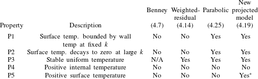
6 Coupling to film equations
The fluid temperature affects the hydrodynamic problem through tangential stresses at the air–fluid surface, and hence only via
 $S(x,t)$
; this coupling to hydrodynamics has been well studied within the context of systems with uniformly heated walls. On the other hand, the heat transfer problem is influenced by the velocity field throughout the fluid layer, and this coupling can become quite intricate. Our aim here is to derive long-wave momentum and heat equations both valid for non-uniform heating.
6.1 Effect of surface temperature on film equations
We use a two-equation, weighted-residual model for the film dynamics, coupling the film height
 $h(x,t)$
and the depth-integrated flux
 $q(x,t)$
, which naturally satisfy
 $$\begin{eqnarray}q(x,t)=\int _{0}^{h(x,t)}u(x,y,t)\,\text{d}y,\quad h_{t}+q_{x}=0,\end{eqnarray}$$
where the second equation follows from mass conservation.
We follow the standard weighted-residual approach, seeking to include surface tension, inertia, axial diffusion and Marangoni stresses. In order to retain second-order terms relating to Marangoni effects, and including some interactions between inertia and Marangoni stresses, we set
 $Re=O(\unicode[STIX]{x1D6FF})$
,
 $Ma=O(\unicode[STIX]{x1D6FF}^{-1})$
,
 $Ca=O(\unicode[STIX]{x1D6FF}^{2})$
and reach
 $$\begin{eqnarray}\displaystyle q+\frac{2}{5}Re\,h^{2}q_{t} & = & \displaystyle \frac{h^{3}}{3}\left(2-2h_{x}\cot \unicode[STIX]{x1D6FD}+\frac{[(1-Ma\,Ca\,S)h_{xx}]_{x}}{Ca}\right)+Re\left(\frac{18q^{2}h_{x}}{35}-\frac{34hqq_{x}}{35}\right)\nonumber\\ \displaystyle & & \displaystyle +\,\left(\frac{8}{5}qh_{x}^{2}-\frac{9}{5}hh_{x}q_{x}-\frac{12}{5}qhh_{xx}+\frac{9}{5}q_{xx}h^{2}\right)-\frac{1}{2}Ma\,h^{2}S_{x}\nonumber\\ \displaystyle & & \displaystyle +\,Ma\,Re\left(\frac{qh^{2}h_{x}S_{x}}{56}+\frac{19h^{3}S_{x}q_{x}}{840}+\frac{3h^{3}qS_{xx}}{112}+\frac{h^{4}S_{xt}}{120}\right)\nonumber\\ \displaystyle & & \displaystyle +\,Ma\left(-\frac{h^{4}S_{xxx}}{10}-\frac{3h_{x}S_{xx}h^{3}}{10}+\frac{3h_{x}^{2}S_{x}h^{2}}{10}-\frac{h_{xx}S_{x}h^{3}}{15}\right)\nonumber\\ \displaystyle & & \displaystyle -\,Ma^{2}Re\left(\frac{19}{1680}h^{4}S_{x}^{2}h_{x}+\frac{5h^{5}S_{x}S_{xx}}{672}\right).\end{eqnarray}$$
In this case the Marangoni number appears both through tangential stresses and as variable surface tension from the normal stress balance.
6.2 Heat transfer through a non-uniform film
The heat equation is affected by film non-uniformity in two ways: the boundary conditions should be applied at
 $y=h(x,t)$
, and the velocity field
 $(u,v)$
appears directly in the heat equation. The first effect here is easy to deal with, but, for the second, we need a suitable characterization of the velocity field. Noting that the derivation of the equation for surface temperature makes use of
 $u$
and its derivatives at the surface, it is reasonable to use the flux-parametrized velocity profile, as is also used in the derivation of the weighted-residual hydrodynamic equations:
 $$\begin{eqnarray}u=\frac{3qy(2h-y)}{2h^{3}},\quad v=\unicode[STIX]{x1D6FF}\hat{v}=\unicode[STIX]{x1D6FF}\left(\frac{3qh_{X}y^{2}(2h-y)}{2h^{4}}-\frac{q_{X}y^{2}(3h-y)}{2h^{3}}\right).\end{eqnarray}$$
This velocity field is incompressible, and obeys
 $u_{y}=0$
and
 $h_{T}=-q_{X}=\hat{v}-uh_{X}$
at
 $y=h$
.
As for the uniform film case, we derive the projected heat equation by posing an expansion of
 $\unicode[STIX]{x1D703}(X,y,T)$
for small
 $\unicode[STIX]{x1D6FF}$
in the form (4.4). The boundary conditions on
 $\unicode[STIX]{x1D703}_{0}$
,
 $\unicode[STIX]{x1D703}_{1}$
and
 $\unicode[STIX]{x1D703}_{2}$
are obtained from expanding the two conditions
 $$\begin{eqnarray}\unicode[STIX]{x1D703}=S(X,T),\quad \unicode[STIX]{x1D703}_{y}-\unicode[STIX]{x1D6FF}^{2}h_{X}\unicode[STIX]{x1D703}_{X}=-Bi\,S(1+\unicode[STIX]{x1D6FF}^{2}h_{X}^{2})^{1/2},\quad \text{on }y=h(X,T),\end{eqnarray}$$
in powers of
 $\unicode[STIX]{x1D6FF}$
. Similarly, the PDEs obeyed by
 $\unicode[STIX]{x1D703}_{0}$
,
 $\unicode[STIX]{x1D703}_{1}$
and
 $\unicode[STIX]{x1D703}_{2}$
are determined from a small-
 $\unicode[STIX]{x1D6FF}$
expansion of
 $$\begin{eqnarray}\unicode[STIX]{x1D6FF}Pe(\unicode[STIX]{x1D703}_{T}+u\unicode[STIX]{x1D703}_{X}+\hat{v}\unicode[STIX]{x1D703}_{y})=\unicode[STIX]{x1D6FF}^{2}\unicode[STIX]{x1D703}_{XX}+\unicode[STIX]{x1D703}_{YY}.\end{eqnarray}$$
We close the model with the condition that
 $\unicode[STIX]{x1D703}(X,0,T)=\unicode[STIX]{x1D6E9}(X,T)$
.
The resulting equation involves time derivatives of the hydrodynamic variables
 $h$
and
 $q$
. We can use
 $h_{T}=-q_{X}$
to eliminate time derivatives of
 $h$
, to reach (in terms of the original variables)
 $$\begin{eqnarray}\displaystyle & & \displaystyle \hspace{-5.0pt}Pe^{2}\left(\frac{1}{24}+\frac{Bi\,h}{120}\right)h^{4}S_{tt}+Pe^{2}\left(\frac{161}{1680}+\frac{29Bi\,h}{1680}\right)qh^{3}S_{xt}\nonumber\\ \displaystyle & & \displaystyle \hspace{-5.0pt}\qquad +\,\left[Pe^{2}q^{2}\left(\frac{239}{4480}+\frac{39Bi\,h}{4480}\right)-\left(\frac{1}{2}+\frac{Bi\,h}{6}\right)\right]h^{2}S_{xx}\nonumber\\ \displaystyle & & \displaystyle \hspace{-5.0pt}\qquad +\,Pe\left[\left(\frac{1}{2}+\frac{Bi\,h}{6}\right)h^{2}+\left(\frac{3}{40}+\frac{17Bi\,h}{560}\right)qh^{2}h_{x}Pe-\left(\frac{13}{120}+\frac{73Bi\,h}{1680}\right)h^{3}q_{x}Pe\right]S_{t}\nonumber\\ \displaystyle & & \displaystyle \hspace{-5.0pt}\qquad +\,\left[\left(\frac{5}{8}+\frac{7Bi\,h}{40}\right)Pe\,q+\left(Pe^{2}q^{2}\left(\frac{239}{4480}+\frac{117Bi\,h}{4480}\right)-(1+Bi\,h)\right)h_{x}\right.\nonumber\\ \displaystyle & & \displaystyle \hspace{-5.0pt}\qquad \left.+\,Pe^{2}\left\{-\left(\frac{173}{4480}+\frac{27Bi\,h}{896}\right)hqq_{x}+\left(\frac{7}{120}+\frac{3Bi\,h}{280}\right)h^{2}q_{t}\right\}\right]hS_{x}\nonumber\\ \displaystyle & & \displaystyle \hspace{-5.0pt}\qquad +\,\left[(1+Bi\,h)+Pe\,Bi\left(\frac{7}{40}hh_{x}q-\frac{9}{40}h^{2}q_{x}\right)+Bi\,h\left(Pe^{2}\frac{39}{4480}q^{2}-\frac{1}{2}\right)(h_{x}^{2}+hh_{xx})\right.\nonumber\\ \displaystyle & & \displaystyle \hspace{-5.0pt}\qquad +\,Bi\,Pe^{2}h^{2}\left.\left(\frac{1331}{40\,320}hq_{x}^{2}-\frac{97}{3360}h_{x}qq_{x}-\frac{271}{13\,440}hqq_{xx}+\frac{3}{280}hh_{x}q_{t}-\frac{1}{84}h^{2}q_{xt}\right)\right]S\nonumber\\ \displaystyle & & \displaystyle \hspace{-5.0pt}\quad =\unicode[STIX]{x1D6E9}(x,t).\end{eqnarray}$$
A substantial simplification arises if the system is steady, as then all derivatives of
 $q$
vanish, as do time derivatives of
 $S$
, leaving
 $$\begin{eqnarray}\displaystyle & & \displaystyle \hspace{-10.00002pt}\left[Pe^{2}q^{2}\left(\frac{239}{4480}+\frac{39Bi\,h}{4480}\right)-\left(\frac{1}{2}+\frac{Bi\,h}{6}\right)\right]h^{2}S_{xx}\nonumber\\ \displaystyle & & \displaystyle \hspace{-10.00002pt}\qquad +\,\left[Pe\,q\left(\frac{5}{8}+\frac{7Bi\,h}{40}\right)+h_{x}\left(Pe^{2}q^{2}\left(\frac{239}{4480}+\frac{117Bi\,h}{4480}\right)-(1+Bi\,h)\right)\right]hS_{x}\nonumber\\ \displaystyle & & \displaystyle \hspace{-10.00002pt}\qquad +\,\left(1+Bi\,h+\frac{7Pe\,Bi}{40}hh_{x}q+Bi\,h\left(Pe^{2}q^{2}\frac{39}{4480}-\frac{1}{2}\right)(h_{x}^{2}+hh_{xx})\right)S\nonumber\\ \displaystyle & & \displaystyle \hspace{-10.00002pt}\quad =\unicode[STIX]{x1D6E9}(x).\end{eqnarray}$$
We can also include the effect of Marangoni stresses on the flow field used to derive the heat equation:
 $$\begin{eqnarray}u=\frac{3qy(2h-y)}{2h^{3}}+\unicode[STIX]{x1D6FF}\frac{Ma\,S_{X}}{4}\frac{y(2h-3y)}{h},\quad \hat{v}=-\int _{0}^{y}u_{X}(x,y^{\prime })\,\text{d}y^{\prime }.\end{eqnarray}$$
For steady states, and assuming that
 $Ma$
and
 $Pe$
are both
 $O(1)$
, the Marangoni stresses have the effect of adding the term
 $$\begin{eqnarray}Pe\,Ma\left(-\frac{h^{3}S_{x}^{2}}{48}+Bi\left(\frac{1}{80}SS_{xx}h^{4}+\frac{1}{240}h^{4}S_{x}^{2}+\frac{7}{240}h^{3}SS_{x}h_{x}\right)\right),\end{eqnarray}$$
to the left-hand side of (6.7). (The expression required to describe Marangoni corrections to the unsteady equation (6.6) is considerably longer.)
7 Steady states subject to localized heating
7.1 Small displacement solutions
In the limit of small
 $Ma$
, we can obtain a solution by linearizing about a flat film. We let
 $$\begin{eqnarray}h=1+Ma\,H\text{e}^{\text{i}kx},\quad q={\textstyle \frac{2}{3}},\quad S={\hat{S}}\text{e}^{\text{i}kx}+O(Ma),\quad \unicode[STIX]{x1D6E9}=\text{e}^{\text{i}kx}.\end{eqnarray}$$
We can analyse the linear solution via a heat transfer problem, which relates
 $\unicode[STIX]{x1D6E9}$
and
 $S$
, and a hydrodynamic problem, which relates
 $S$
and
 $h$
. We solve the hydrodynamic problem (6.2) at
 $O(Ma)$
to obtain
 $$\begin{eqnarray}H=\frac{\text{i}k{\hat{S}}}{4}\frac{1-{\displaystyle \frac{\text{i}kRe}{28}}-{\displaystyle \frac{k^{2}}{5}}}{1-{\displaystyle \frac{\text{i}k\cot \unicode[STIX]{x1D6FD}}{3}}+{\displaystyle \frac{4\text{i}kRe}{35}}+{\displaystyle \frac{4k^{2}}{5}}-{\displaystyle \frac{\text{i}k^{3}}{6Ca}}}.\end{eqnarray}$$
The heat transfer problem, to determine
 ${\hat{S}}$
, is exactly the linear problem discussed in § 5.
For small displacements of the fluid surface, we can use an Orr–Sommerfeld analysis to solve both the Navier–Stokes and heat equations and hence determine the equivalent full 2-D surface displacement. The results are shown in figure 11 for comparison with the long-wave results, in a case with strong surface tension and low Reynolds number, so that the base flow is stable. The long-wave results are in very good agreement with those from the linearized 2-D system. Note that the half-width of the strip heating profile has been increased from
 $X=2$
to
 $X=5$
; this leads to increased deflection of
 $h(x)$
and makes the surface shape easier to visualize.
Solutions at small
 $Ma$
(with
 $h(x)=1+Ma\,{\hat{h}}(x)+O(Ma^{2})$
) for the strip heating profile (5.1) with
 $Re=1$
,
 $Ca=0.01$
,
 $Bi=0$
,
 $\unicode[STIX]{x1D6FD}=\unicode[STIX]{x03C0}/4$
, with (a)
 $Pe=1$
and (b)
 $Pe=10$
, in a periodic domain with period 100. The full 2-D result is shown by the black solid line, the red dashed line is the long-wave result, and the blue line indicates the smoothed strip heater profile with half-width
 $X=5$
. Note that the heating strip leads to the formation of a capillary ridge above the upstream edge of the heater.
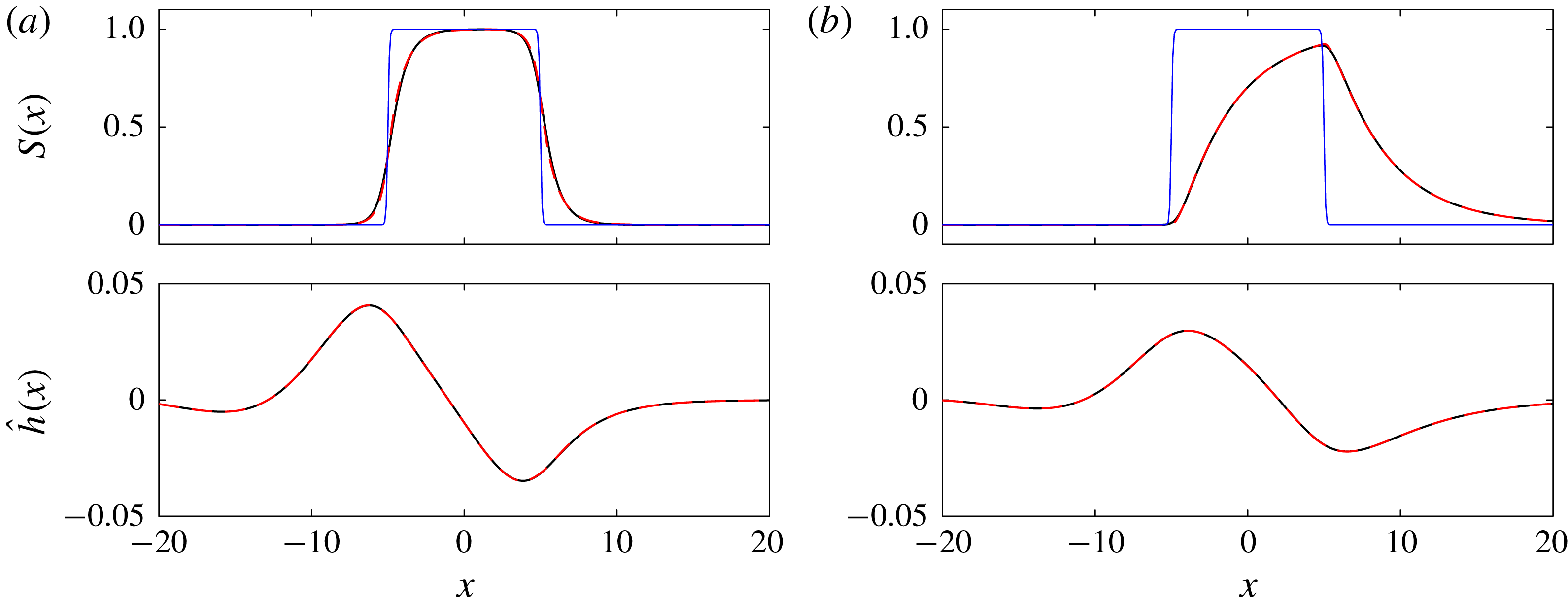
7.2 Finite-amplitude solutions
At small
 $Ma$
, the heat problem is exactly the same as that for flat films. Hence, to test the validity of the dependence of (6.7) on
 $h$
and
 $q$
, we must increase the deformation, most easily achieved by increasing
 $Ma$
. For large-amplitude solutions, we solve numerically in a periodic domain, applying the strip-like distribution (5.2) for
 $\unicode[STIX]{x1D6E9}$
and obtain steady states by continuation in
 $Ma$
from
 $h=1$
at
 $Ma=0$
, subject to the constraint that the mean layer height is fixed at 1. Results using the long-wave equations (6.2) and (6.7), computed using the bifurcation and continuation transfer package Auto 07p (Doedel & Oldman Reference Doedel and Oldman2009), are shown in figure 12. With all other parameters fixed, we find that increasing
 $Ma$
increases the surface deformation
 $h$
, accompanied by only small changes in the surface temperature profile
 $S$
.
Long-wave solutions for
 $Ma=1,5,10,15,10$
and
 $25$
at
 $Pe=1,5,10$
and
 $Bi=0,1$
, with
 $\unicode[STIX]{x1D6E9}$
given by (5.1) with
 $X=5$
and
 $\unicode[STIX]{x1D70E}=10$
. The equations solved are (6.2) and (6.7), excluding the
 $Pe\,Ma$
terms in (6.9). Dots show oomph-lib solutions of the 2-D Navier–Stokes equation and heat equation, while solid lines represent the long-wave model. All solutions are obtained by continuation from
 $Ma=0$
, except for the dashed solutions shown for the two
 $Pe=5$
cases, which are obtained by continuation in
 $Pe$
and
 $Ma$
from solutions at
 $Pe=1$
,
 $Ma=25$
. We cannot obtain long-wave solutions in the interval
 $14.67<Ma<14.88$
for
 $Bi=0$
,
 $Pe=5$
. The interval without solutions for the case
 $Bi=1$
,
 $Pe=5$
is much larger, with no converged long-wave solutions in
 $7.79<Ma<17.67$
.

Solutions are available for a wide range of
 $Ma$
(at least up to
 $Ma=25$
), except for the two cases with
 $Pe=5$
. This value of
 $Pe=5$
is close to the critical
 $Pe$
for a uniform film with
 $h=1$
,
 $q=2/3$
for both
 $Bi=0$
(where
 $Pe^{\ast }=4.592$
) and
 $Bi=1$
(where
 $Pe^{\ast }=4.917$
), so that the coefficient of
 $S_{xx}$
, at
 $h=1$
and
 $q=2/3$
, is small but non-zero in both cases. Therefore, it is possible that the coefficient of
 $S_{xx}$
in the nonlinear calculations,
 $$\begin{eqnarray}\left[Pe^{2}q^{2}\left(\frac{239}{4480}+\frac{39Bi\,h}{4480}\right)-\left(\frac{1}{2}+\frac{Bi\,h}{6}\right)\right]h^{2},\end{eqnarray}$$
may vanish as
 $q$
and
 $h$
vary.
For
 $Bi=0$
, the sign of (7.3) is a function only of
 $Pe$
and
 $q$
, and would vanish at
 $q=0.6123$
for
 $Pe=5$
, for example. As
 $q$
is spatially constant in steady calculations, in fact this would mean that the coefficient of
 $S_{xx}$
vanishes everywhere in the domain simultaneously if
 $q$
exactly coincides with the critical value, but the equation would be non-singular for all other
 $q$
. In the case
 $Pe=5$
,
 $Bi=0$
, continuation from
 $Ma=0$
yields solutions up to
 $Ma=14.68$
, where
 $q=0.614208$
. In order to obtain solutions for larger
 $Ma$
, we use continuation from
 $Pe=1$
,
 $Bi=0$
, first increasing
 $Pe$
and then decreasing
 $Ma$
. Using this method, the Auto code yields converged solutions down to
 $Ma=14.88$
.
In contrast, for
 $Bi\neq 0$
, the dependence of the sign of the coefficient of (7.3) on
 $h$
means that the coefficient can vanish at some points in the domain but not others, and hence, for sufficiently large surface deformation, we expect the ODE (6.7) to have one or more singular points. Fixing
 $Pe=5$
,
 $Bi=1$
and
 $q=2/3$
, (7.3) would vanish at points where
 $h=1.326$
. However, the calculations shown in figure 12 are performed with a constraint on layer height, so that
 $q$
decreases slightly as
 $Ma$
increases. For
 $Bi=1$
,
 $Pe=5$
, the last converged solution when increasing
 $Ma$
from zero is for
 $Ma=7.7899$
, where
 $q=0.66237$
and the maximum value of
 $h$
is
 $1.15829$
. Using a continuation method from solutions at large
 $Ma$
for
 $Pe=1$
, we can also obtain solutions at
 $Pe=5$
,
 $Bi=1$
for
 $Ma>17.64$
, where
 $q=0.64321$
and the minimum value of
 $h$
is 0.684856. Comparison of these values of
 $Pe$
,
 $Bi$
,
 $h$
and
 $q$
with (7.3) suggests that the border of the region where we can compute solutions does indeed correspond to conditions where the coefficient of
 $S_{xx}$
locally vanishes.
The finite-amplitude calculations require 2-D Navier–Stokes simulations for validation. Steady solutions are calculated using the finite-element library oomph-lib (Heil & Hazel Reference Heil, Hazel, Schäfer and Bungartz2006). In this computation, Marangoni effects are created by specifying the variation of surface tension with temperature, leading to effects in both the normal and tangential components of the dynamic boundary condition, consistent with the boundary conditions (2.16) and (2.17) used to derive our long-wave equations. The air layer is treated as a region of constant pressure and temperature, and heat loss is parametrized by the same Biot-number condition as we used to derive the model. The Navier–Stokes calculations are performed in closed conditions: a periodic domain with mean layer height 1.
Several of the long-wave calculations are in remarkably good quantitative agreement with the full nonlinear Navier–Stokes results. In particular, for
 $Bi=1$
, the long-wave results shown in figure 12 are in excellent agreement for
 $h(x)$
across the range of
 $Ma$
where they exist. The predictions for
 $S(x)$
are also in good agreement at
 $Bi=1$
, capturing the notable increase in
 $S$
at the downstream end of the heater as
 $Ma$
increases. The agreement for
 $Bi=0$
is less good than for
 $Bi=1$
; this is likely due to the generally reduced surface temperatures for larger
 $Bi$
leading to smaller variations in
 $h(x)$
at the same
 $Ma$
and hence less significant nonlinearity. For
 $Ma\gtrapprox 10$
and
 $Bi=0$
at the larger
 $Pe$
, the predictions for the upstream fluid ridge have the wrong shape when compared to the 2-D nonlinear results. This may be related to the observation that, while the long-wave results correctly predict an increasingly rapid decay of
 $S(x)$
downstream of the heater as
 $Ma$
increases, they do not capture the slowing of the upstream decay, which should lead to increasingly important upstream influence regions.
Long-wave solutions (solid lines) and Navier–Stokes calculations (dotted lines) for
 $Ma=1,5,10,15,20$
and
 $25$
at
 $Pe=1,5,10$
and
 $Bi=0,1$
, with
 $\unicode[STIX]{x1D6E9}$
given by (5.1) with
 $X=5$
and
 $\unicode[STIX]{x1D70E}=10$
. These results include the
 $Pe\,Ma$
interactions in (6.9). All solutions shown here are computed by continuation from
 $Ma=0$
at fixed
 $Pe$
and
 $Bi$
. This continuation method does not yield long-wave solutions above
 $Ma=9.388$
for
 $Pe=5$
,
 $Bi=0$
, above
 $Ma=18.00$
for
 $Pe=10$
,
 $Bi=0$
, and above
 $Ma=8.240$
for
 $Pe=5$
,
 $Bi=1$
; in each case this last converged solution is plotted with dashed lines.

Similar calculations including the Marangoni influences on the heat equation itself via (6.9) are shown in figure 13. For
 $Pe=1$
,
 $Bi=0$
, these correction terms lead to better agreement for
 $S(x)$
, particularly just upstream of the heating strip. There is also slightly improved agreement for
 $h(x)$
. However, for larger
 $Pe$
, the inclusion of
 $Pe\,Ma$
terms via (6.9) reduces the range of
 $Ma$
over which solutions can be obtained. In particular, note that for
 $Bi=0$
, we obtain solutions at
 $Pe=5$
up to
 $Ma=9.39$
and at
 $Pe=10$
up to
 $Ma=18.0$
. In both cases, the last converged solution is associated with strong deviations from the Navier–Stokes results for
 $S(x)$
at the upstream edge of the heating strip. The full 2-D solutions persist without qualitative changes in behaviour until at least
 $Ma=25$
.
We can isolate the effects of
 $Pe\,Ma$
interactions in a much simpler problem: the zero-
 $Ca$
, zero-
 $Re$
limit of strong surface tension, where the normal component of the dynamic boundary condition implies simply that the surface is flat, but Marangoni stresses drive an internal flow due to the tangential stress balance. If
 $S(x)$
is known, the full equations for
 $u$
and
 $v$
are linear:
 $$\begin{eqnarray}u=y(2-y)-\unicode[STIX]{x1D713}_{y},\quad v=\unicode[STIX]{x1D713}_{x},\quad \unicode[STIX]{x1D6FB}^{4}\unicode[STIX]{x1D713}=0,\quad \text{in }0<y<1,\end{eqnarray}$$
subject to
 $u=v=0$
on
 $y=0$
, and
 $u_{y}=-Ma\,S_{x}$
,
 $v=0$
on
 $y=1$
. The unique solution for
 $u$
and
 $v$
with
 $S$
given can be obtained by Fourier transforms. However, the coupled problem is nonlinear, as the surface temperature
 $S(x)=\unicode[STIX]{x1D703}(x,1)$
is determined by the heat equation, which itself involves the velocity field
 $$\begin{eqnarray}Pe\left(u\frac{\unicode[STIX]{x2202}\unicode[STIX]{x1D703}}{\unicode[STIX]{x2202}x}+v\frac{\unicode[STIX]{x2202}\unicode[STIX]{x1D703}}{\unicode[STIX]{x2202}y}\right)=\frac{\unicode[STIX]{x2202}^{2}\unicode[STIX]{x1D703}}{\unicode[STIX]{x2202}x^{2}}+\frac{\unicode[STIX]{x2202}^{2}\unicode[STIX]{x1D703}}{\unicode[STIX]{x2202}y^{2}},\end{eqnarray}$$
subject to
 $\unicode[STIX]{x1D703}=\unicode[STIX]{x1D6E9}(x)$
on
 $y=0$
and
 $\unicode[STIX]{x1D703}_{y}=-Bi\,\unicode[STIX]{x1D703}$
on
 $y=1$
.
Within the long-wave limit, the structure of the equations for this limiting case is similar to that of the full problem. The steady velocity field induced by a surface temperature
 $S(x)$
is given by
 $$\begin{eqnarray}u=y(2-y)+\frac{Ma}{4}y(2-3y)S_{x},\quad v=\frac{Ma}{4}S_{xx}y^{2}(y-1).\end{eqnarray}$$
It is straightforward to verify that the ‘projected’ heat equation can also be obtained by setting
 $h=1$
and
 $q=2/3$
in the equivalent non-uniform equation (6.7) with the addition of (6.9):
 $$\begin{eqnarray}\displaystyle & & \displaystyle \left[Pe^{2}\left(\frac{239}{10\,080}+\frac{13Bi}{3360}\right)-\left(\frac{1}{2}+\frac{Bi}{6}\right)\right]S_{xx}+\left[Pe\left(\frac{5}{12}+\frac{7Bi}{60}\right)\right]S_{x}\nonumber\\ \displaystyle & & \displaystyle \quad +\,\left(1+Bi\right)S+Pe\,Ma\left(-\frac{S_{x}^{2}}{48}+Bi\left(\frac{SS_{xx}}{80}+\frac{S_{x}^{2}}{240}\right)\right)=\unicode[STIX]{x1D6E9}(x).\end{eqnarray}$$
Without the
 $Pe\,Ma$
term, the velocity field is independent of
 $S$
, and so if
 $h$
is known,
 $u$
and
 $v$
are also known, the heat equation is linear, and the full and long-wave heat equations each have a unique solution for
 $S$
. However, with non-zero
 $Pe\,Ma$
, there is no reason to expect a unique solution in either the full or long-wave system.
Calculations for
 $S(x)$
in the strong surface tension limit, as
 $Ma$
increases from zero at
 $Pe=10$
with (a)
 $Bi=0$
and (b)
 $Bi=1$
, with
 $\unicode[STIX]{x1D6E9}$
given by (5.1) with
 $X=5$
and
 $\unicode[STIX]{x1D70E}=10$
. The long-wave results (solid lines) are obtained by solving (7.7) directly, while the 2-D results (dotted lines) are from Navier–Stokes calculations with
 $Ca=10^{-5}$
. For
 $Bi=0$
, we show additionally the 2-D results for
 $Ma=100$
.

We can apply the same strip heating profile as in figure 13 and calculate the surface temperature profile in the strong surface tension limit. The long-wave and full 2-D results (calculated using the full Navier–Stokes code with
 $Ca=10^{-5}$
) are shown in figure 14. We find that the long-wave solution branch for
 $Pe=10$
,
 $Bi=0$
persists to
 $Ma\approx 40$
, but the maximum value of
 $S$
increases with increasing
 $Ma$
and in fact crosses 1 at
 $Ma\approx 32$
, thus violating property P5, which should still hold in this limit. For relatively small
 $Ma$
(up to
 $Ma=20$
for
 $Bi=0$
and up to
 $Ma=40$
for
 $Bi=1$
), the full 2-D results are quite similar to the long-wave results, with a broadening region of constant temperature above the strip. Beyond these Marangoni numbers, the 2-D results predict that this region continues to broaden, and the surface is always hottest above the downstream end of the strip. At the very largest
 $Ma$
(
 $Ma=100$
for
 $Bi=1$
), we start to see the appearance of a reversal in the direction of the temperature gradient, in qualitative agreement with the long-wave results. However, the long-wave model predicts that this feature should emerge at much lower
 $Ma$
and be much larger in magnitude by
 $Ma=100$
. The long-wave models hence lose accuracy at around
 $Ma=20$
, with
 $Pe=10$
, by which point the combination
 $Pe\,Ma$
is clearly not small. Hence, if better agreement is required at these parameters, the equations should be rederived under the assumption of large
 $Pe\,Ma$
with respect to the long-wave parameter
 $\unicode[STIX]{x1D6FF}$
, likely introducing further nonlinear interactions.
8 Conclusion
We have explored in detail the formulation of long-wave models for predicting the effect of localized wall heating on surface temperature, and via variation of surface tension with temperature, on the dynamics of falling liquid films. This problem can be split into two components: the relationship between surface temperature
 $S$
and wall temperature
 $\unicode[STIX]{x1D6E9}$
, which is moderated by flow, and the relationship between surface temperature and film dynamics. The latter coupling occurs via Marangoni stresses in the momentum balance, and has already been studied in a variety of contexts. However, the first part, on the transmission of localized heating through a uniform or non-uniform film, is not yet well understood and our paper represents the first comprehensive study in this area.
We began our analysis of the heat transmission problem by deriving thermodynamic constraints for the full 2-D heat equation subject to a uniform Nusselt flow. We proved five properties: (P1) the magnitude of temperature variations at the fluid surface must be less than that imposed at the wall; (P2) at short wavelength, the surface feels no temperature variation; (P3) in the absence of imposed heating, the film should decay to uniform temperature; (P4) there can be no local extrema of the temperature field inside the fluid layer; and (P5) the surface temperature must be bounded by the extrema of the wall and air temperature.
In previous studies of film patterning by imposed steady heating, most authors have chosen to use only the leading-order long-wave model
 $S=\unicode[STIX]{x1D6E9}/(1+Bi\,h)$
. This leading-order model takes no account of advection or streamwise diffusion, and predicts instantaneous reaction to any change in wall temperature. The leading-order model is especially inaccurate in the large-
 $Pe$
regime that would apply if the film Reynolds number is large enough for the flow to be unstable.
In many isothermal falling liquid film studies, the hydrodynamic model used is second-order-accurate or higher with respect to the long-wave parameter, and so we focused here on thermal models that are also second-order-accurate. If the film is uniform (always attainable with
 $Ma=0$
), the surface temperature equation should be linear in
 $S$
and
 $\unicode[STIX]{x1D6E9}$
, and there are five free parameters in choosing a second-order-accurate model with at most second-order derivatives of
 $S$
and
 $\unicode[STIX]{x1D6E9}$
with respect to space and time. The most obvious of these models is a Benney-type model, yielding the surface temperature explicitly in terms of
 $\unicode[STIX]{x1D6E9}$
,
 $\unicode[STIX]{x1D6E9}_{x}$
,
 $\unicode[STIX]{x1D6E9}_{t}$
,
 $\unicode[STIX]{x1D6E9}_{xx}$
,
 $\unicode[STIX]{x1D6E9}_{xt}$
and
 $\unicode[STIX]{x1D6E9}_{tt}$
. However, although this model is quantitatively accurate in the long-wave limit, it is divergent when evaluated in the short-wave limit, gives completely inaccurate results when applied to a smoothed heating strip, and fails all applicable thermodynamic tests. For the purely hydrodynamic isothermal problem, the deficiencies of the Benney model can be remedied by use of a weighted-residual model, which leads to an additional degree of freedom in the system. However, application of the same methodology for the heat equation is less successful; although it indeed leads to an evolution equation for
 $S$
rather than an explicit expression, it still fails most of the thermodynamic tests because it still relies upon derivatives of
 $\unicode[STIX]{x1D6E9}$
, which is not even required to be smooth in the full 2-D heat equation.
We are therefore led to seek a second-order model that gives
 $S$
implicitly, but with only
 $\unicode[STIX]{x1D6E9}$
and not its derivatives appearing as a source function. There is a unique model of this form among the class of linear second-order-accurate models. We showed that this model can be obtained systematically by solving for a temperature field that exactly satisfies the two boundary conditions at the surface along with the bulk equation. We can then ‘read off’ the wall temperature in terms of
 $S$
and its derivatives. Requiring that this wall temperature coincides with the imposed function leads to an evolution equation for
 $S$
. The resulting model always satisfies P1–P3.
Having focused our attention on this new ‘projected’ model, we proceeded to examine its behaviour across a wider range of parameters, for both uniform and non-uniform films. For uniform films, the equation is always hyperbolic, but the direction of its characteristics depends on
 $Pe$
. For
 $Pe$
below a critical value
 $Pe^{\ast }$
, one family of characteristics travels upstream and the other downstream and, for both steady and time-dependent systems, a localized heating strip affects the surface temperature both upstream and downstream. For
 $Pe$
above the critical value, both families of characteristics travel downstream, and a heating strip has strictly downstream influence. The value of
 $Pe^{\ast }$
depends slightly on
 $Bi$
, ranging from 4.592 to 6.563 as
 $Bi$
ranges from zero to infinity. If the film is uniform and the system is steady, the projected model reduces to a second-order, constant-coefficient ODE for the steady surface temperature corresponding to a given wall profile. Furthermore, solving this ODE via variation of parameters allows us to show that, except in a subset of the region
 $Bi>3.87$
, non-negative wall temperature leads to non-negative surface temperature; thus P5 holds.
Our new model is unique among second-order models in satisfying P1–P3 and P5, but still does not guarantee that the corresponding internal temperature profile (supplied as part of the derivation) is thermodynamically consistent with property P4. By considering cases with sharp wall temperature gradients, with
 $Pe$
close to
 $Pe^{\ast }$
, we can construct counterexamples to P4. The question of negative surface and internal temperatures also arises in the study of travelling waves on films subject to uniform heating, and has not been conclusively avoided there either. However, we should also note that the constraints on modelling imposed by heterogeneous heating do not apply for uniform heating, so that a wider class of models could be relevant in that case.
Having examined the performance of our new model against the five thermodynamic properties, we next considered how film non-uniformity modifies the temperature equation. The derivation follows in a similar way to that for a uniform film, but it requires explicit parametrization of the velocity field, and can in general lead to a rather complicated governing equation. If
 $h$
and
 $q$
are predetermined, the evolution equation is again hyperbolic, but, as the coefficients in the long-wave heat equation depend on
 $h$
and
 $q$
, the direction of the characteristics may evolve with the solution.
As the Marangoni number is increased for the case of steady heating, our model predicts increasing surface deflection, in accordance with full Navier–Stokes results. The variations in
 $h(x)$
are accompanied by minor changes in
 $S(x)$
, at least up to
 $Ma\approx 20$
. There is no evidence of bifurcations at smaller
 $Ma$
, though calculations for
 $Pe$
near to
 $Pe^{\ast }$
do not converge for all
 $Ma$
, due to the development of local singularities in the equations associated with the change in criticality of the equations.
At larger
 $Ma$
, the full 2-D results still show only mild changes in
 $S(x)$
. Some of these features are well predicted by the long-wave models; for example, the increase in surface temperature at the downstream end of the heater for non-zero
 $Bi$
. We can seek to improve the agreement by including Marangoni corrections in the velocity field used to derive the heat equation; a nonlinear effect associated with the combination
 $Pe\,Ma$
. At small
 $Pe$
, these corrections indeed lead to better agreement, but for
 $Pe=10$
and
 $Ma\approx 20$
, the long-wave model yields unphysical predictions such as an increasingly hot free-surface near the upstream end of the heater. This upstream heating effect emerges even if film non-uniformity is eliminated by considering the limit of very large surface tension, where the film surface should be flat, and can lead to very hot regions on the air–fluid surface, violating P5. These predictions can likely be improved to some extent by allowing
 $Pe\,Ma$
to be asymptotically large in the derivation of the long-wave model, but such broad applicability would come at the cost of further increase to the model complexity.
In our analysis we have assumed throughout that the temperature at the wall is exactly specified. However, in physical implementation it is more likely that the boundary condition would involve either a specification of the heat flux or some linear combination of temperature and heat flux (conceivably coupled to another thermal problem within the wall such as considered by Dallaston, Tseluiko & Kalliadasis (Reference Dallaston, Tseluiko and Kalliadasis2016)). Our modelling methodology can be easily extended to these more general boundary conditions (see appendix A). The derivation again involves expanding the temperature field about the surface values; the model is closed by the condition that the surface-based expansion for
 $\unicode[STIX]{x1D703}$
be consistent with whatever boundary conditions are required at the wall. We note that the analysis would still hold even if parameters in the boundary condition, for example, the thermal conductivity of the wall, are themselves variable. This would also allow long-wave access to boundary conditions of mixed type, and more accurately reflect the experimental set-up for the analysis of ridge instability, where a heating strip of known heat flux is embedded in either an insulating wall, or one kept at a constant temperature away from the heater.
The long-wave modelling methodology developed here should serve as a useful modelling framework for a number of problems, including our motivating problem of control via spatially and temporally varying heating, and also the canonical system of the spanwise instabilities of the capillary ridge induced by a single heating strip. Our analysis can also be modified to account for a nonlinear dependence of surface tension on temperature. However, we have not considered the case of temperature-dependent viscosity, which remains a significant challenge.
Acknowledgements
We are grateful to the referees for valuable comments and suggestions and to Professor D. T. Papageorgiou from Imperial College for numerous stimulating discussions. We acknowledge financial support from the London Engineering and Physical Sciences Research Council of the UK through grants nos EP/K041134/1, EP/M021556/1, EP/K008595/1, EP/L020564/1, EP/K023154/1 and EP/P026044/1 and from the Leverhulme Trust via the Early Career Fellowship ECF-2018-536.
Supplementary material
The data for this paper are in the figures, and source files for these are available in the supplementary information available at https://doi.org/10.1017/jfm.2019.580.
Appendix A. Heat transfer through a uniform film subject to imposed heat flux at the wall
In this study, we have assumed throughout that the temperature of the rigid wall is exactly specified. We can use the same methodology to form an equivalent to our new projected model for the case where the heat flux is specified at the wall, i.e.
 $$\begin{eqnarray}\unicode[STIX]{x1D703}_{y}|_{y=0}=-F(x,t).\end{eqnarray}$$
We formulate the same expansion of the temperature field about the air–fluid surface as in § 4.3, using (4.5), (4.17) and (4.18), or the equivalent expressions for the non-uniform film. The difference is that the model is now closed by requiring that the expansion of
 $\unicode[STIX]{x1D703}$
must obey (A 1). We obtain the following equation:
 $$\begin{eqnarray}\displaystyle & & \displaystyle \hspace{-10.0pt}-Bi\,S-Pe\left(\left(1+\frac{Bi}{2}\right)S_{t}+\left(\frac{2}{3}+\frac{Bi}{4}\right)S_{x}\right)+S_{xx}\left(\left(1+\frac{Bi}{2}\right)-Pe^{2}\left(\frac{13}{210}+\frac{17Bi}{1440}\right)\right)\nonumber\\ \displaystyle & & \displaystyle \hspace{-10.0pt}\quad -\,S_{xt}Pe^{2}\left(\frac{13}{60}+\frac{17Bi}{360}\right)-S_{tt}Pe^{2}\left(\frac{1}{6}+\frac{Bi}{24}\right)=-F(x,t)={\mathcal{L}}_{N}S(x,t).\end{eqnarray}$$
This equation is very similar to that for specified wall temperature in that it is always hyperbolic and changes from subcritical to supercritical at a critical value of
 $Pe$
which depends on
 $Bi$
.
In the more general case where the boundary condition at the wall involves a linear combination of
 $\unicode[STIX]{x1D703}$
and its normal derivative,
 $$\begin{eqnarray}\unicode[STIX]{x1D6FC}\unicode[STIX]{x1D703}|_{y=0}-\unicode[STIX]{x1D6FE}\unicode[STIX]{x1D703}_{y}|_{y=0}=F(x,t),\end{eqnarray}$$
the surface temperature equation is simply the corresponding linear combination of the equation with specified temperature and with specified flux,
 $$\begin{eqnarray}\{\unicode[STIX]{x1D6FC}{\mathcal{L}}_{P}-\unicode[STIX]{x1D6FE}{\mathcal{L}}_{N}\}S(x,t)=F(x,t),\end{eqnarray}$$
where the operator
 ${\mathcal{L}}_{P}$
is defined for the Dirichlet problem in (4.19) and
 ${\mathcal{L}}_{N}$
for the Neumann problem in (A 2). Note that this derivation does not require that
 $\unicode[STIX]{x1D6FC}$
and
 $\unicode[STIX]{x1D6FE}$
be constant in either time or space, so that for example the boundary conditions could be taken to be perfectly insulating over some regions of the wall and at specified temperature in others. This combination would allow direct simulation of the formation and spanwise instability of a capillary ridge due to a localized heating strip.


 Open access

