1 Introduction
Superhydrophobic surfaces have received considerable attention in recent years due to their low wettability and reduced viscous drag (Ou, Perot & Rothstein Reference Ou, Perot and Rothstein2004). Typically they consist of a no-slip surface patterned with micrometre structures such as pillars or grooves. A liquid in the Cassie state – where gas is trapped in the microcavities – experiences low shear stress on the liquid–gas interfaces (menisci) and a reduced overall viscous drag, frequently measured in terms of an apparent slip length. Flows over many different superhydrophobic microstructure geometries have been studied extensively, with experiments, numerical solutions, and analytical techniques (Lauga & Stone Reference Lauga and Stone2003; Cottin-Bizonne et al. Reference Cottin-Bizonne, Barentin, Charlaix, Bocquet and Barrat2004; Ou & Rothstein Reference Ou and Rothstein2005).
An important class of surfaces is a parallel array of ridges aligned with the flow direction, owing to their advantage in heat transfer performance compared to pillars (Enright et al. Reference Enright, Hodes, Salamon and Muzychka2014), and advantage in drag reduction compared to transverse (oriented perpendicular to the flow direction) ridges (Teo & Khoo Reference Teo and Khoo2009). The particular geometry of the structures, and the interfaces that span them, have a great effect on the resulting drag reduction. Most initial analytical and computational studies assumed that the menisci are flat for simplicity, but they can be highly curved due to the high pressure gradients required in experiments (Ou & Rothstein Reference Ou and Rothstein2005). Experiments for transverse ridges by Steinberger et al. (Reference Steinberger, Cottin-Bizonne, Kleimann and Charlaix2007) showed that the slip length can become negative, indicating flow degradation, if the meniscus protrusion into the liquid is too large. This motivated Davis & Lauga (Reference Davis and Lauga2009) to develop an analytical model for shear flow over transverse ridges, confirming this dependence on curvature. Crowdy (Reference Crowdy2010) extended the model to shear flow over longitudinal ridges, where the slip length remains positive but with a considerable dependence on the protrusion angle. These studies made the so-called dilute approximation, i.e. that the menisci were spaced widely apart, which was recently extended to higher-order accuracy (Crowdy Reference Crowdy2016). The opposing limit of densely packed menisci (small solid fraction) was considered by Schnitzer (Reference Schnitzer2017). Also in this limit, Ybert et al. (Reference Ybert, Barentin, Cottin-Bizonne, Joseph and Bocquet2007) found slip length scaling laws consistent with their numerical results, and captured the often neglected effects of molecular slip, and shear stress exerted by the gas.
When the parallel ridges are taken to pattern one or both walls of a channel or pipe, only numerical or experimental studies have been able to account for significant meniscus curvature. Sbragaglia & Prosperetti (Reference Sbragaglia and Prosperetti2007) considered a channel with longitudinal ridges on one wall and accounted for small meniscus curvature using boundary perturbation. They found analytical formulae only for an infinite channel thickness, and Kirk, Hodes & Papageorgiou (Reference Kirk, Hodes and Papageorgiou2017) extended these formulae to ridges on both walls, but included all higher-order corrections. When the curvature is not small, which is true for applications involving liquid metals (Lam, Hodes & Enright Reference Lam, Hodes and Enright2015), a detailed study for longitudinal ridges on one channel wall was conducted by Teo & Khoo (Reference Teo and Khoo2010) using a finite-element method. They assessed the accuracy of the boundary perturbation, but also showed that the slip length can become negative for large protrusion, as for transverse ridges, when channel thicknesses are low enough – behaviour not predicted by the formulae for shear flows in the previous paragraph.
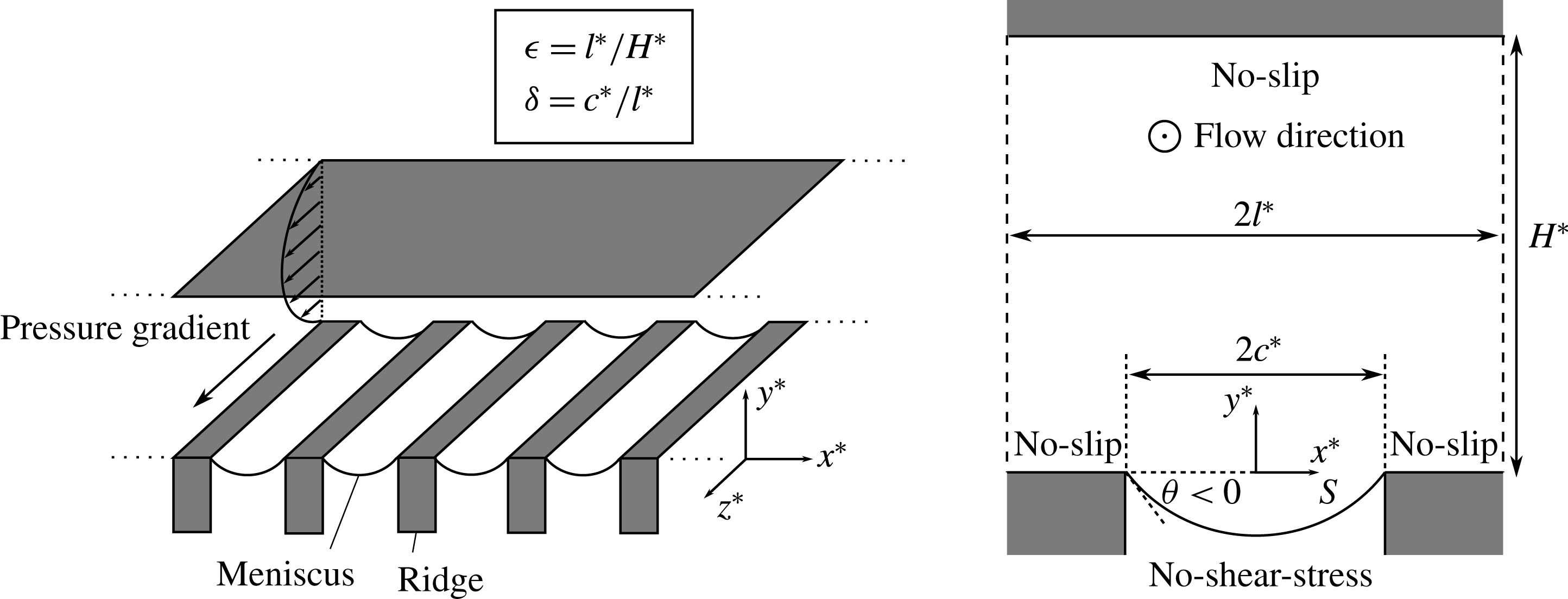
Schematic of the pressure-driven channel flow aligned with a periodic array of ridges, period
 $2l^{\ast }$
, and groove width
 $2c^{\ast }$
. Circular-cross-section menisci contact the ridge corner at angle
 $\unicode[STIX]{x1D703}$
(with
 $\unicode[STIX]{x1D703}<0$
corresponding to downward protrusion). The distance from ridge tips to the opposing wall is
 $H^{\ast }$
.

In analysing flows over parallel ridges, many asymptotic limits of geometric length scales have been employed. Other flows over substrates with transverse variation, such as gravity-driven rivulets, have been studied extensively and successfully with asymptotic methods, including slow streamwise variation (Wilson & Duffy Reference Wilson and Duffy1998) or transverse stresses due to external air flow (Sullivan et al.
Reference Sullivan, Paterson, Wilson and Duffy2012). Neglecting the gas in the cavity, consider a channel of height
 $H^{\ast }$
with parallel ridges of period
 $2l^{\ast }$
and cavity width
 $2c^{\ast }$
patterning one wall, as in figure 1, or both walls symmetrically. (Asterisks denote dimensional quantities.) The pressure difference between the liquid and gas causes the menisci to form circular arcs, protruding into or out of the cavities. There are three length ratios that describe the geometry: (i)
 $\unicode[STIX]{x1D716}=l^{\ast }/H^{\ast }$
, the ratio of ridge period to channel height; (ii)
 $\unicode[STIX]{x1D6FF}=c^{\ast }/l^{\ast }$
, the slip fraction or ratio of groove width to ridge period; (iii)
 $\unicode[STIX]{x1D703}$
, the protrusion angle that the meniscus makes with the horizontal at the corners of the ridges (
 $\unicode[STIX]{x1D703}>0$
corresponds to protrusion into the liquid).
Sbragaglia & Prosperetti (Reference Sbragaglia and Prosperetti2007) considered
 $|\unicode[STIX]{x1D703}|\ll 1$
, with no restriction on
 $\unicode[STIX]{x1D716}$
or
 $\unicode[STIX]{x1D6FF}$
; however, their analytical results were only for an unbounded shear flow, corresponding to
 $\unicode[STIX]{x1D716}=0$
. The dilute (Davis & Lauga Reference Davis and Lauga2009; Crowdy Reference Crowdy2010, Reference Crowdy2016) and dense (Schnitzer Reference Schnitzer2017) meniscus packing assumptions correspond to
 $\unicode[STIX]{x1D6FF}\ll 1$
and
 $1-\unicode[STIX]{x1D6FF}\ll 1$
, respectively, but previous work is only for
 $\unicode[STIX]{x1D716}=0$
. The lack of analytical models for curvature in channels (
 $\unicode[STIX]{x1D716},\unicode[STIX]{x1D703}\neq 0$
) makes tasks such as channel design and optimisation time consuming. Consequently, the slip length formulae for unbounded flows are often used for channels far outside their validity if the menisci are in fact curved (Maynes et al.
Reference Maynes, Webb, Crockett and Solovjov2013; Enright et al.
Reference Enright, Hodes, Salamon and Muzychka2014; Maynes & Crockett Reference Maynes and Crockett2014). Accurate formulae would be especially useful for future 3D considerations, where numerical optimisation is infeasible. In addition to computational savings, they enable one to directly look at special limits, e.g.
 $\unicode[STIX]{x1D703}\rightarrow \pm \unicode[STIX]{x03C0}/2$
. Experiments are constrained by the surface tension of the liquid, and thus given a (maximum) restriction on
 $\unicode[STIX]{x1D703}$
, formulae can immediately give a geometry that maximises slip.
In this paper we present solutions for flow in a channel with longitudinal ridges on one or both walls for finite channel heights, i.e.
 $\unicode[STIX]{x1D716}\neq 0$
, that are valid for any protrusion angle
 $\unicode[STIX]{x1D703}$
, and extend the shear-flow solutions of Crowdy (Reference Crowdy2016). We consider the limit of small period to height ratio,
 $\unicode[STIX]{x1D716}\ll 1$
, using matched asymptotic expansions as per Hodes et al. (Reference Hodes, Kirk, Karamanis and MacLachlan2017), who considered a flat meniscus. Two successive approximations in Crowdy (Reference Crowdy2016) for the non-dimensional shear-flow slip length
 $\unicode[STIX]{x1D706}=\unicode[STIX]{x1D706}^{\ast }/l^{\ast }$
in the small-slip-fraction limit,
 $\unicode[STIX]{x1D6FF}=c^{\ast }/l^{\ast }\ll 1$
, are
 $$\begin{eqnarray}\displaystyle & \displaystyle \unicode[STIX]{x1D706}_{0}=\unicode[STIX]{x1D6FF}^{2}\frac{3\unicode[STIX]{x03C0}^{3}-4\unicode[STIX]{x03C0}^{2}\unicode[STIX]{x1D703}+2\unicode[STIX]{x03C0}\unicode[STIX]{x1D703}^{2}}{12(\unicode[STIX]{x03C0}-\unicode[STIX]{x1D703})^{2}},\quad \unicode[STIX]{x1D706}_{1}=\frac{\unicode[STIX]{x1D706}_{0}}{1-{\displaystyle \frac{\unicode[STIX]{x03C0}}{6}}\unicode[STIX]{x1D706}_{0}}, & \displaystyle\end{eqnarray}$$
with
 $\unicode[STIX]{x1D706}_{0}$
the leading-order approximation, and
 $\unicode[STIX]{x1D706}_{1}$
a more accurate approximation correct up to at least
 $O(\unicode[STIX]{x1D6FF}^{4})$
. The non-dimensional slip length for a channel with ridges on one wall and a smooth no-slip surface on the other is denoted
 $\unicode[STIX]{x1D6FD}=\unicode[STIX]{x1D6FD}^{\ast }/H^{\ast }$
, to distinguish it from
 $\unicode[STIX]{x1D706}$
. It is defined as the effective slip length that realises the same flow rate per period as the actual flow. The main result of this paper is an extension of
 $\unicode[STIX]{x1D706}_{1}$
to the formula
 $$\begin{eqnarray}\displaystyle & \displaystyle \unicode[STIX]{x1D6FD}={\displaystyle \frac{\unicode[STIX]{x1D716}\unicode[STIX]{x1D706}_{1}-\unicode[STIX]{x1D716}^{2}\unicode[STIX]{x1D6FF}^{3}I\left(1+\displaystyle {\displaystyle \frac{\unicode[STIX]{x03C0}}{6}}\unicode[STIX]{x1D706}_{1}\right)\left[2+\left(\unicode[STIX]{x1D716}^{2}-{\displaystyle \frac{\unicode[STIX]{x03C0}}{6}}\unicode[STIX]{x1D716}\right)\unicode[STIX]{x1D6FF}^{3}I\right]+(1+\unicode[STIX]{x1D716}\unicode[STIX]{x1D706}_{1})\unicode[STIX]{x1D716}^{3}\unicode[STIX]{x1D6FF}^{4}(F-G)}{1+\unicode[STIX]{x1D716}^{2}\unicode[STIX]{x1D6FF}^{3}I\left(1+\displaystyle {\displaystyle \frac{\unicode[STIX]{x03C0}}{6}}\unicode[STIX]{x1D706}_{1}\right)\left[2+\left(\unicode[STIX]{x1D716}^{2}-{\displaystyle \frac{\unicode[STIX]{x03C0}}{6}}\unicode[STIX]{x1D716}\right)\unicode[STIX]{x1D6FF}^{3}I\right]-(1+\unicode[STIX]{x1D716}\unicode[STIX]{x1D706}_{1})\unicode[STIX]{x1D716}^{3}\unicode[STIX]{x1D6FF}^{4}(F-G)}}, & \displaystyle\end{eqnarray}$$
where
 $$\begin{eqnarray}\displaystyle & \displaystyle I(\unicode[STIX]{x1D703})=16\sin \unicode[STIX]{x1D703}\int _{0}^{\unicode[STIX]{x03C0}/2}\frac{\tan ^{2\unicode[STIX]{x1D6FC}}\unicode[STIX]{x1D719}[\cos \unicode[STIX]{x1D703}\tan ^{2\unicode[STIX]{x1D6FC}}\unicode[STIX]{x1D719}+2\tan ^{\unicode[STIX]{x1D6FC}}\unicode[STIX]{x1D719}+\cos \unicode[STIX]{x1D703}]\,\text{d}\unicode[STIX]{x1D719}}{[\tan ^{2\unicode[STIX]{x1D6FC}}\unicode[STIX]{x1D719}+2\cos \unicode[STIX]{x1D703}\tan ^{\unicode[STIX]{x1D6FC}}\unicode[STIX]{x1D719}+1]^{3}},\quad \unicode[STIX]{x1D6FC}=\frac{2}{\unicode[STIX]{x03C0}}(\unicode[STIX]{x03C0}-\unicode[STIX]{x1D703}), & \displaystyle \nonumber\\ \displaystyle & & \displaystyle\end{eqnarray}$$
 $$\begin{eqnarray}\displaystyle & \displaystyle F(\unicode[STIX]{x1D703})=\csc ^{4}\unicode[STIX]{x1D703}\left[\unicode[STIX]{x1D703}\left(3+2\cos 2\unicode[STIX]{x1D703}\right)-{\textstyle \frac{7}{3}}\sin 2\unicode[STIX]{x1D703}-{\textstyle \frac{1}{12}}\sin 4\unicode[STIX]{x1D703}\right], & \displaystyle\end{eqnarray}$$
and
 $G(\unicode[STIX]{x1D703})$
is given up to quadrature by (5.7), or by the correlation (5.10). The result for a similar channel with longitudinal ridges on both walls is simpler, but given in terms of the same functions,
 $$\begin{eqnarray}\displaystyle & \displaystyle \unicode[STIX]{x1D6FD}^{(sym)}=\unicode[STIX]{x1D716}\unicode[STIX]{x1D706}_{1}-\unicode[STIX]{x1D716}^{2}\unicode[STIX]{x1D6FF}^{3}I\left(1+\frac{\unicode[STIX]{x03C0}}{6}\unicode[STIX]{x1D706}_{1}\right)\left(2-\frac{\unicode[STIX]{x03C0}}{6}\unicode[STIX]{x1D716}\unicode[STIX]{x1D6FF}^{3}I\right)+\unicode[STIX]{x1D716}^{3}\unicode[STIX]{x1D6FF}^{4}(F-G). & \displaystyle\end{eqnarray}$$
Formulae (1.2) and (1.5) elucidate the differences between the shear-flow and channel flow slip lengths when the menisci are curved. They are explicit and valid for the entire range of protrusion angles
 $\unicode[STIX]{x1D703}\in [-\unicode[STIX]{x03C0}/2,\unicode[STIX]{x03C0}/2]$
, and a very large range of
 $\unicode[STIX]{x1D716}$
. Formula (1.2) is compared against finite-element computations and the accuracy in
 $\unicode[STIX]{x1D6FF}$
is similar to that of
 $\unicode[STIX]{x1D706}_{1}$
: up to
 $\unicode[STIX]{x1D716}=0.5$
, the maximum relative errors for
 $\unicode[STIX]{x1D6FF}=0.5$
and
 $0.75$
are
 ${\sim}0.8\,\%$
and
 ${\sim}8\,\%$
, respectively. This accuracy holds even up to
 $\unicode[STIX]{x1D716}=2.5$
, where the meniscus can touch the opposite wall and
 $\unicode[STIX]{x1D6FD}$
becomes negative, as seen by Teo & Khoo (Reference Teo and Khoo2010).
The matched asymptotics procedure for
 $\unicode[STIX]{x1D716}\ll 1$
reduces the problem to a shear flow in an inner region near the ridges with a forcing on the meniscus, the solution of which gives an exponentially accurate solution for the channel flow. We only consider the dilute limit
 $\unicode[STIX]{x1D6FF}\ll 1$
of this inner problem, but the asymptotic decomposition holds for any periodic structuring, and can be extended to other limits or to include other physical effects.
2 Governing equations
We will focus on steady, fully developed flow in a parallel plate channel with longitudinal ridges on one wall, as in figure 1. The analysis for the case of longitudinal ridges on both channel walls is almost identical, and can be found in the supplementary material available at https://doi.org/10.1017/jfm.2018.73. The flow is assumed unidirectional,
 $\boldsymbol{u}^{\ast }=(0,0,w^{\ast }(x^{\ast },y^{\ast }))$
, governed by
 $\unicode[STIX]{x1D707}\unicode[STIX]{x1D6FB}^{2}w^{\ast }=\unicode[STIX]{x2202}p^{\ast }/\unicode[STIX]{x2202}z^{\ast }$
in the cross-plane, with a constant pressure gradient
 $-\unicode[STIX]{x2202}p^{\ast }/\unicode[STIX]{x2202}z^{\ast }$
and viscosity
 $\unicode[STIX]{x1D707}$
. We need only consider one period window,
 $x^{\ast }\in [-l^{\ast },l^{\ast }]$
, with a cavity located at
 $x^{\ast }\in [-c^{\ast },c^{\ast }]$
. The gas phase and streamwise curvature variation are neglected. The non-dimensional velocity and lengths are defined as
 $w=-(2\unicode[STIX]{x1D707}/H^{\ast 2})(\unicode[STIX]{x2202}p^{\ast }/\unicode[STIX]{x2202}z^{\ast })^{-1}w^{\ast }$
and
 $(x,y)=(x^{\ast },y^{\ast })/H^{\ast }$
, giving the following non-dimensional problem in the cross-plane,
 $$\begin{eqnarray}\displaystyle & \displaystyle \unicode[STIX]{x1D6FB}^{2}w=-2, & \displaystyle\end{eqnarray}$$
where
 $\unicode[STIX]{x1D6FB}^{2}=\unicode[STIX]{x2202}^{2}/\unicode[STIX]{x2202}x^{2}+\unicode[STIX]{x2202}^{2}/\unicode[STIX]{x2202}y^{2}$
, with no-slip at the top of the domain,
 $$\begin{eqnarray}\displaystyle & \displaystyle w=0,\quad \text{on }y=1,\,x\in [-\unicode[STIX]{x1D716},\unicode[STIX]{x1D716}] & \displaystyle\end{eqnarray}$$
and mixed no-slip/no-shear-stress conditions at the bottom of the domain,
 $$\begin{eqnarray}\displaystyle & \displaystyle w=0,\quad \text{on }y=0,\,x\notin [-\unicode[STIX]{x1D716}\unicode[STIX]{x1D6FF},\unicode[STIX]{x1D716}\unicode[STIX]{x1D6FF}] & \displaystyle\end{eqnarray}$$
 $$\begin{eqnarray}\displaystyle & \displaystyle \boldsymbol{n}\boldsymbol{\cdot }\unicode[STIX]{x1D735}w=0,\quad \text{on the meniscus }S, & \displaystyle\end{eqnarray}$$
where
 $\boldsymbol{n}$
is the unit normal pointing into the liquid. Periodic or symmetry boundary conditions, i.e.
 $\unicode[STIX]{x2202}w/\unicode[STIX]{x2202}x=0$
, apply at
 $x=\pm \unicode[STIX]{x1D716}$
.
3 The limit of large channel height to ridge period,
 $\unicode[STIX]{x1D716}\ll 1$

The procedure of the matched asymptotic expansion for
 $\unicode[STIX]{x1D716}=l^{\ast }/H^{\ast }\ll 1$
is similar to that in Hodes et al. (Reference Hodes, Kirk, Karamanis and MacLachlan2017), to which we refer the reader for a more detailed description. In the limit
 $\unicode[STIX]{x1D716}\rightarrow 0$
, the domain decomposes into an outer region where
 $y=O(1)$
and the flow is 1D and parabolic, and an inner region near the ridges where
 $y=O(\unicode[STIX]{x1D716})$
and the
 $x$
variation is present.
3.1 Outer region:
$y=O(1)$

After rescaling the transverse coordinate,
 $X=x/\unicode[STIX]{x1D716}$
, and substituting a regular asymptotic expansion
 $w\sim w_{0}+\unicode[STIX]{x1D716}w_{1}+\cdots =\sum _{n=0}^{\infty }\unicode[STIX]{x1D716}^{n}w_{n}$
with
 $X,y,w_{n}=O(1)$
into (2.1) and applying periodicity at each order, Hodes et al. showed that each
 $w_{n}$
is only a function of
 $y$
, i.e.
 $w_{n}=w_{n}(y)$
for all
 $n\geqslant 0$
. This means
 $w$
is independent of
 $X$
in the outer region to all algebraic orders in
 $\unicode[STIX]{x1D716}$
. Integrating at each order and applying only the condition (2.2) at
 $y=1$
gives the one-dimensional outer solution
 $$\begin{eqnarray}\displaystyle & \displaystyle w=-y^{2}+y+B(\unicode[STIX]{x1D716})(1-y), & \displaystyle\end{eqnarray}$$
where
 $B(\unicode[STIX]{x1D716})$
is the (asymptotic) series
 $B(\unicode[STIX]{x1D716}):=\sum _{n\geqslant 0}^{\infty }B_{n}\unicode[STIX]{x1D716}^{n}$
and the
 $B_{n}$
are
 $O(1)$
constants.
The mixed boundary conditions at the bottom of the domain cannot be satisfied by (3.1) since it has no
 $X$
dependence, so an inner solution is needed. It is important to notice that the form of the outer solution is independent of the particular structure of the substrate at
 $y=0$
, the periodicity in
 $X$
so far being the only requirement for the outer solution to take the form (3.1).
3.2 Inner region:
$y=O(\unicode[STIX]{x1D716})$

The effect of the ridges becomes significant when
 $y$
is comparable to the ridge period, i.e.
 $y\sim x=\unicode[STIX]{x1D716}X=O(\unicode[STIX]{x1D716})$
, and both terms of the Laplacian balance in (2.1). We introduce
 $Y=y/\unicode[STIX]{x1D716}$
, which is
 $O(1)$
as
 $\unicode[STIX]{x1D716}\rightarrow 0$
in the inner region. The solution here, denoted
 $w=W(X,Y)$
, satisfies
 $$\begin{eqnarray}\displaystyle & \displaystyle \frac{\unicode[STIX]{x2202}^{2}W}{\unicode[STIX]{x2202}X^{2}}+\frac{\unicode[STIX]{x2202}^{2}W}{\unicode[STIX]{x2202}Y^{2}}=-2\unicode[STIX]{x1D716}^{2}. & \displaystyle\end{eqnarray}$$
In inner variables
 $(X,Y)$
, the conditions at the bottom of the domain are identical to (2.3) and (2.4), with the meniscus occupying
 $X\in [-\unicode[STIX]{x1D6FF},\unicode[STIX]{x1D6FF}]$
in a period window
 $[-1,1]$
. Using Van Dyke’s matching principle for matching with the outer region,
 $W$
as
 $Y\rightarrow \infty$
must be identical to (3.1) with
 $y=\unicode[STIX]{x1D716}Y$
substituted, giving
 $$\begin{eqnarray}\displaystyle & \displaystyle W\sim -\unicode[STIX]{x1D716}^{2}Y^{2}+\unicode[STIX]{x1D716}Y+B(\unicode[STIX]{x1D716})(1-\unicode[STIX]{x1D716}Y),\quad \text{as }Y\rightarrow \infty . & \displaystyle\end{eqnarray}$$
As (3.1) holds to all algebraic orders in
 $\unicode[STIX]{x1D716}$
, (3.3) must hold to all orders in
 $Y$
. It can be shown (Hodes et al.
Reference Hodes, Kirk, Karamanis and MacLachlan2017) that
 $W=0$
for
 $\unicode[STIX]{x1D716}=0$
, implying
 $B(\unicode[STIX]{x1D716})=O(\unicode[STIX]{x1D716}),$
or
 $\hat{B}(\unicode[STIX]{x1D716})=B(\unicode[STIX]{x1D716})/\unicode[STIX]{x1D716}=O(1)$
.
This inner problem can be reduced to Laplace’s equation in a semi-infinite domain, driven by a shear flow, with the following substitution,
 $$\begin{eqnarray}\displaystyle & \displaystyle W=-\unicode[STIX]{x1D716}^{2}Y^{2}+[1-\unicode[STIX]{x1D716}\hat{B}(\unicode[STIX]{x1D716})]\unicode[STIX]{x1D716}\widehat{W}. & \displaystyle\end{eqnarray}$$
Along with periodicity or symmetry conditions at
 $X=\pm 1$
, the problem for
 $\widehat{W}$
is given by
 $$\begin{eqnarray}\displaystyle & \displaystyle \frac{\unicode[STIX]{x2202}^{2}\widehat{W}}{\unicode[STIX]{x2202}X^{2}}+\frac{\unicode[STIX]{x2202}^{2}\widehat{W}}{\unicode[STIX]{x2202}Y^{2}}=0, & \displaystyle\end{eqnarray}$$
 $$\begin{eqnarray}\displaystyle & \displaystyle \widehat{W}=0,\quad \text{on }Y=0,\,X\notin [-\unicode[STIX]{x1D6FF},\unicode[STIX]{x1D6FF}] & \displaystyle\end{eqnarray}$$
 $$\begin{eqnarray}\displaystyle & \displaystyle \boldsymbol{n}\boldsymbol{\cdot }\unicode[STIX]{x1D735}_{XY}\widehat{W}=[1+\unicode[STIX]{x1D716}\hat{\unicode[STIX]{x1D706}}(\unicode[STIX]{x1D716})]\,\boldsymbol{n}\boldsymbol{\cdot }\unicode[STIX]{x1D735}_{XY}(\unicode[STIX]{x1D716}Y^{2}),\quad \text{on the meniscus }S & \displaystyle\end{eqnarray}$$
 $$\begin{eqnarray}\displaystyle & \displaystyle \widehat{W}\sim Y+\hat{\unicode[STIX]{x1D706}}(\unicode[STIX]{x1D716}),\quad \text{as }Y\rightarrow \infty , & \displaystyle\end{eqnarray}$$
where
 $\hat{\unicode[STIX]{x1D706}}(\unicode[STIX]{x1D716})=\hat{B}(\unicode[STIX]{x1D716})/(1-\unicode[STIX]{x1D716}\hat{B}(\unicode[STIX]{x1D716}))=O(1)$
, and
 $\unicode[STIX]{x1D735}_{XY}=(\unicode[STIX]{x2202}/\unicode[STIX]{x2202}X,\unicode[STIX]{x2202}/\unicode[STIX]{x2202}Y)$
is the gradient in the inner coordinates.
We remark that
 $\widehat{W}$
is
 $O(1)$
but depends on
 $\unicode[STIX]{x1D716}$
. A formal expansion of
 $\widehat{W}$
in
 $\unicode[STIX]{x1D716}$
is unnecessary, as any solution method at
 $O(\unicode[STIX]{x1D716})$
can be used to solve the unexpanded problem directly. The above problem is similar to that considered by Crowdy (Reference Crowdy2010, Reference Crowdy2016) but with an additional non-constant forcing on the meniscus. This term is not present if the meniscus is flat or if we restrict to leading order (
 $\unicode[STIX]{x1D716}=0$
), in which case
 $\widehat{W}$
corresponds exactly to the unbounded shear flow over the same surface, and
 $\hat{\unicode[STIX]{x1D706}}$
is the associated slip length. For a meniscus shape
 $Y(X)$
, the forcing term can be written
 $$\begin{eqnarray}\displaystyle & \displaystyle \boldsymbol{n}\boldsymbol{\cdot }\unicode[STIX]{x1D735}_{XY}(\unicode[STIX]{x1D716}Y^{2})=\frac{2\unicode[STIX]{x1D716}Y}{(1+{Y^{\prime }}^{2})^{1/2}}, & \displaystyle\end{eqnarray}$$
where
 $Y^{\prime }(X)=\text{d}Y/\text{d}X$
. If
 $Y(X)$
is a circular arc, this is a known function of
 $X$
.
Finally, just as in Hodes et al., the solution is the same in the outer region as the overlap region, so a composite solution uniformly valid throughout the entire domain is simply the inner solution:
 $$\begin{eqnarray}\displaystyle & \displaystyle w_{comp}=W=-y^{2}+\frac{\unicode[STIX]{x1D716}}{1+\unicode[STIX]{x1D716}\hat{\unicode[STIX]{x1D706}}}\widehat{W}. & \displaystyle\end{eqnarray}$$
4 Solution of inner problem: small slip fraction,
$\unicode[STIX]{x1D6FF}\ll 1$

We make no further approximation in
 $\unicode[STIX]{x1D716}$
, and to solve the inner problem given by (3.5)–(3.8) we consider the additional limit of small slip fraction,
 $\unicode[STIX]{x1D6FF}=c^{\ast }/l^{\ast }\ll 1$
, or the dilute limit. The problem Crowdy (Reference Crowdy2010, Reference Crowdy2016) considered corresponds to (3.5)–(3.8) with
 $\unicode[STIX]{x1D716}=0$
– a shear-free meniscus. Therefore we present an extension of Crowdy (Reference Crowdy2016) to account for this inhomogeneity – the full details are given in the supplementary material. Since
 $\widehat{W}$
is harmonic, let
 ${\hat{h}}(z)$
with
 $z=X+\text{i}Y$
be its complex potential such that
 $\widehat{W}=\text{Im}\{{\hat{h}}(z)\}$
. If the complex potential for the flow over a single such meniscus is
 ${\hat{h}}_{s}(z)$
, then repeating Crowdy’s superposition arguments gives the first two approximations to the periodic case as:
 $$\begin{eqnarray}\displaystyle & \displaystyle {\hat{h}}_{0}(z)={\hat{h}}_{s}(z)+\hat{\unicode[STIX]{x1D706}}_{0}\left[\frac{2}{\unicode[STIX]{x03C0}z}-\cot \left(\frac{\unicode[STIX]{x03C0}z}{2}\right)\right],\quad \hat{\unicode[STIX]{x1D706}}_{0}=\frac{\unicode[STIX]{x1D706}_{0}-\unicode[STIX]{x1D716}\unicode[STIX]{x1D6FF}^{3}I}{1+\unicode[STIX]{x1D716}^{2}\unicode[STIX]{x1D6FF}^{3}I}, & \displaystyle\end{eqnarray}$$
 $$\begin{eqnarray}\displaystyle & \displaystyle {\hat{h}}_{1}(z)={\hat{h}}_{s}(z)+\hat{\unicode[STIX]{x1D706}}_{1}\left[\frac{2}{\unicode[STIX]{x03C0}z}-\cot \left(\frac{\unicode[STIX]{x03C0}z}{2}\right)+\frac{\unicode[STIX]{x03C0}}{6}(h_{s}(z)-z)\right],\quad \hat{\unicode[STIX]{x1D706}}_{1}=\frac{\unicode[STIX]{x1D706}_{1}-\unicode[STIX]{x1D716}\unicode[STIX]{x1D6FF}^{3}\left(1+{\displaystyle \frac{\unicode[STIX]{x03C0}}{6}}\unicode[STIX]{x1D706}_{1}\right)I}{1+\unicode[STIX]{x1D716}^{2}\unicode[STIX]{x1D6FF}^{3}\left(1+{\displaystyle \frac{\unicode[STIX]{x03C0}}{6}}\unicode[STIX]{x1D706}_{1}\right)I}, & \displaystyle \nonumber\\ \displaystyle & & \displaystyle\end{eqnarray}$$
where
 $\unicode[STIX]{x1D706}_{0}$
,
 $\unicode[STIX]{x1D706}_{1}$
,
 $I(\unicode[STIX]{x1D703})$
are (1.1), (1.3), and
 $h_{s}(z)$
is the potential for a single shear-free meniscus. It can be shown that (4.1) and (4.2) satisfy the requirements for
 ${\hat{h}}(z)$
with errors of
 $O(\unicode[STIX]{x1D6FF}^{3})$
and
 $O(\unicode[STIX]{x1D6FF}^{5})$
, respectively. The potential
 ${\hat{h}}_{s}(z)$
is found by conformally mapping the flow domain to an auxiliary
 $\unicode[STIX]{x1D701}$
-domain (upper half-disk) via
 $$\begin{eqnarray}\displaystyle & \displaystyle \unicode[STIX]{x1D701}(z)=\frac{(z/\unicode[STIX]{x1D6FF}-1)^{1/\unicode[STIX]{x1D6FC}}-(z/\unicode[STIX]{x1D6FF}+1)^{1/\unicode[STIX]{x1D6FC}}}{(z/\unicode[STIX]{x1D6FF}-1)^{1/\unicode[STIX]{x1D6FC}}+(z/\unicode[STIX]{x1D6FF}+1)^{1/\unicode[STIX]{x1D6FC}}},\quad \unicode[STIX]{x1D6FC}=\frac{2}{\unicode[STIX]{x03C0}}(\unicode[STIX]{x03C0}-\unicode[STIX]{x1D703}), & \displaystyle\end{eqnarray}$$
then analytically continuing to the unit disk and invoking the Poisson integral formula. The result takes the form
 $$\begin{eqnarray}\displaystyle {\hat{h}}_{s}(z(\unicode[STIX]{x1D701}))=\underbrace{\frac{\unicode[STIX]{x1D6FF}}{\unicode[STIX]{x1D6FC}}\left(\unicode[STIX]{x1D701}-\unicode[STIX]{x1D701}^{-1}\right)}_{\displaystyle h_{s}}+\frac{1}{2\unicode[STIX]{x03C0}\text{i}}\int _{|\unicode[STIX]{x1D701}^{\prime }|=1}\frac{\text{d}\unicode[STIX]{x1D701}^{\prime }}{\unicode[STIX]{x1D701}^{\prime }}\frac{\unicode[STIX]{x1D701}^{\prime }+\unicode[STIX]{x1D701}}{\unicode[STIX]{x1D701}^{\prime }-\unicode[STIX]{x1D701}}f(\unicode[STIX]{x1D701}^{\prime }),\quad f(\unicode[STIX]{x1D701})=\left\{\begin{array}{@{}ll@{}}\unicode[STIX]{x1D712}[z(\unicode[STIX]{x1D701})]\quad & \text{Im}(\unicode[STIX]{x1D701})\geqslant 0,\\ \unicode[STIX]{x1D712}[z(\unicode[STIX]{x1D701}^{-1})]\quad & \text{Im}(\unicode[STIX]{x1D701})<0,\end{array}\right. & & \displaystyle \nonumber\\ \displaystyle & & \displaystyle\end{eqnarray}$$
where
 $\unicode[STIX]{x1D712}(z)$
is the real integral
 $[1+\unicode[STIX]{x1D716}\hat{\unicode[STIX]{x1D706}}(\unicode[STIX]{x1D716})]\int ^{X}2\unicode[STIX]{x1D716}Y(X^{\prime })\,\text{d}X^{\prime }$
written in terms of
 $z=X+\text{i}Y$
.
5 Apparent slip length formula
The apparent slip length
 $\unicode[STIX]{x1D6FD}$
of a channel flow is defined, following Lauga & Stone (Reference Lauga and Stone2003), by equating the flow rate per unit width,
 $Q$
, with that of an effective Navier slip profile
 $$\begin{eqnarray}\displaystyle & \displaystyle w_{NS}=-y^{2}+\frac{y+\unicode[STIX]{x1D6FD}}{1+\unicode[STIX]{x1D6FD}},\quad Q_{NS}=\frac{1}{2\unicode[STIX]{x1D716}}\int _{-\unicode[STIX]{x1D716}}^{\unicode[STIX]{x1D716}}\int _{0}^{1}w_{NS}\,\text{d}y\,\text{d}x=\frac{2}{3}-\frac{1}{2(1+\unicode[STIX]{x1D6FD})}, & \displaystyle\end{eqnarray}$$
which satisfies a Navier slip condition
 $w_{NS}=\unicode[STIX]{x1D6FD}\,\text{d}w_{NS}/\text{d}y$
at
 $y=0$
, and
 $w_{NS}=0$
at
 $y=1$
. The outer solution (3.1), written in terms of
 $\hat{\unicode[STIX]{x1D706}}$
, already takes the form of a Navier slip profile:
 $$\begin{eqnarray}\displaystyle & \displaystyle w=-y^{2}+\frac{y+\unicode[STIX]{x1D716}\hat{\unicode[STIX]{x1D706}}}{1+\unicode[STIX]{x1D716}\hat{\unicode[STIX]{x1D706}}}. & \displaystyle\end{eqnarray}$$
However, this does not imply that
 $\unicode[STIX]{x1D716}\hat{\unicode[STIX]{x1D706}}$
is our approximation to
 $\unicode[STIX]{x1D6FD}$
, since the flow rate
 $Q=(1/2\unicode[STIX]{x1D716})\int _{D}w(x,y)\,\text{d}x\,\text{d}y$
will have contributions from the inner region. The effective Navier slip profile must be integrated over a rectangular cross-section, but the actual flow cross-section is not rectangular when the meniscus is curved. This difference in cross-section complicates the relationship between
 $\unicode[STIX]{x1D6FD}$
and
 $\unicode[STIX]{x1D716}\hat{\unicode[STIX]{x1D706}}$
, and there is a contribution from the change in area.
To calculate
 $Q$
we derive a reciprocal result from Green’s second identity in the cross-section
 $D$
with
 $1/2y^{2}$
and
 $w(x,y)$
(which satisfies (2.1)–(2.4)) as the chosen functions. The identity states that
 $$\begin{eqnarray}\displaystyle & \displaystyle \int _{D}\left[w\unicode[STIX]{x1D6FB}^{2}\left(\frac{1}{2}y^{2}\right)-\frac{1}{2}y^{2}\unicode[STIX]{x1D6FB}^{2}w\right]\,\text{d}A=-\int _{\unicode[STIX]{x2202}D}\left[w\frac{\unicode[STIX]{x2202}}{\unicode[STIX]{x2202}n}\left(\frac{1}{2}y^{2}\right)-\frac{1}{2}y^{2}\frac{\unicode[STIX]{x2202}w}{\unicode[STIX]{x2202}n}\right]\,\text{d}s, & \displaystyle\end{eqnarray}$$
where
 $\unicode[STIX]{x2202}/\unicode[STIX]{x2202}n$
is the inward normal derivative. Now,
 $\unicode[STIX]{x1D6FB}^{2}w=-2$
,
 $\unicode[STIX]{x1D6FB}^{2}(y^{2}/2)=1$
, and the only surviving boundary integrals are along
 $y=1$
and the meniscus,
 $$\begin{eqnarray}\displaystyle & \displaystyle \int _{D}w\,\text{d}A+\int _{D}y^{2}\,\text{d}A=\int _{y=1}-\frac{1}{2}\frac{\unicode[STIX]{x2202}w}{\unicode[STIX]{x2202}y}\,\text{d}x-\int _{S}w\frac{\unicode[STIX]{x2202}}{\unicode[STIX]{x2202}n}\left(\frac{1}{2}y^{2}\right)\,\text{d}s. & \displaystyle\end{eqnarray}$$
Substituting the outer solution at
 $y=1$
, the inner solution on the meniscus, and rearranging,
 $$\begin{eqnarray}\displaystyle & \displaystyle 2\unicode[STIX]{x1D716}Q=-\int _{D}y^{2}\,\text{d}A+2\unicode[STIX]{x1D716}\left[1-\frac{1}{2(1+\unicode[STIX]{x1D716}\hat{\unicode[STIX]{x1D706}})}\right]+\int _{S}y^{3}\frac{\unicode[STIX]{x2202}y}{\unicode[STIX]{x2202}n}\,\text{d}s-\frac{\unicode[STIX]{x1D716}}{1+\unicode[STIX]{x1D716}\hat{\unicode[STIX]{x1D706}}}\int _{S}\widehat{W}y\frac{\unicode[STIX]{x2202}y}{\unicode[STIX]{x2202}n}\,\text{d}s. & \displaystyle\end{eqnarray}$$
Each integral is straightforwardly evaluated from the geometry except the last, which requires the inner solution on the meniscus. Using the approximation (4.2), and neglecting terms of
 $O(\unicode[STIX]{x1D6FF}^{7})$
, this becomes
 $Q=Q_{outer}+Q^{\prime }$
, where
 $Q_{outer}$
is the flow rate of the outer slip profile down to
 $y=0,$
and
 $Q^{\prime }$
the extra contribution from the change in shape,
 $$\begin{eqnarray}\displaystyle & \displaystyle Q_{outer}=\frac{2}{3}-\frac{1}{2(1+\unicode[STIX]{x1D716}\hat{\unicode[STIX]{x1D706}})},\quad Q^{\prime }=-\frac{\unicode[STIX]{x1D716}^{2}\unicode[STIX]{x1D6FF}^{3}}{2(1+\unicode[STIX]{x1D716}\hat{\unicode[STIX]{x1D706}})}I(\unicode[STIX]{x1D703})+\frac{1}{2}\unicode[STIX]{x1D716}^{3}\unicode[STIX]{x1D6FF}^{4}[F(\unicode[STIX]{x1D703})-G(\unicode[STIX]{x1D703})]+O(\unicode[STIX]{x1D6FF}^{7}), & \displaystyle \nonumber\\ \displaystyle & & \displaystyle\end{eqnarray}$$
where
 $I(\unicode[STIX]{x1D703})$
,
 $F(\unicode[STIX]{x1D703})$
are (1.3), (1.4). Then
 $G(\unicode[STIX]{x1D703})$
is given by the integral
 $$\begin{eqnarray}\displaystyle & & \displaystyle \displaystyle G(\unicode[STIX]{x1D703})=\int _{0}^{\unicode[STIX]{x03C0}}\,\text{d}\unicode[STIX]{x1D719}\,K(\unicode[STIX]{x1D719};\unicode[STIX]{x1D703})\unicode[STIX]{x2A0D}_{-\unicode[STIX]{x03C0}}^{\unicode[STIX]{x03C0}}\frac{\text{d}\unicode[STIX]{x1D713}}{2\unicode[STIX]{x03C0}}\cot \left(\frac{\unicode[STIX]{x1D719}-\unicode[STIX]{x1D713}}{2}\right)g(\unicode[STIX]{x1D713};\unicode[STIX]{x1D703}),\end{eqnarray}$$
 $$\begin{eqnarray}\displaystyle & & \displaystyle \displaystyle K(\unicode[STIX]{x1D719};\unicode[STIX]{x1D703})=4\unicode[STIX]{x1D6FC}\sin \unicode[STIX]{x1D703}\frac{\tan ^{2\unicode[STIX]{x1D6FC}}(\unicode[STIX]{x1D719}/2)[\cos \unicode[STIX]{x1D703}+2\tan ^{\unicode[STIX]{x1D6FC}}(\unicode[STIX]{x1D719}/2)+\cos \unicode[STIX]{x1D703}\tan ^{2\unicode[STIX]{x1D6FC}}(\unicode[STIX]{x1D719}/2)]}{\sin \unicode[STIX]{x1D719}[1+2\cos \unicode[STIX]{x1D703}\tan ^{\unicode[STIX]{x1D6FC}}(\unicode[STIX]{x1D719}/2)+\tan ^{2\unicode[STIX]{x1D6FC}}(\unicode[STIX]{x1D719}/2)]^{3}},\end{eqnarray}$$
 $$\begin{eqnarray}\displaystyle & & \displaystyle \displaystyle g(\unicode[STIX]{x1D713};\unicode[STIX]{x1D703})=\csc ^{2}\unicode[STIX]{x1D703}\,\text{i}\log \left[\text{i}\frac{\text{e}^{\text{i}\unicode[STIX]{x1D703}/2}+\text{e}^{-\text{i}\unicode[STIX]{x1D703}/2}\tan ^{\unicode[STIX]{x1D6FC}}(|\unicode[STIX]{x1D713}|/2)}{\text{e}^{-\text{i}\unicode[STIX]{x1D703}/2}+\text{e}^{\text{i}\unicode[STIX]{x1D703}/2}\tan ^{\unicode[STIX]{x1D6FC}}(|\unicode[STIX]{x1D713}|/2)}\right]\nonumber\\ \displaystyle & & \displaystyle +\,\csc \unicode[STIX]{x1D703}\frac{[1-\tan ^{2\unicode[STIX]{x1D6FC}}(|\unicode[STIX]{x1D713}|/2)][\cos \unicode[STIX]{x1D703}+2\cos 2\unicode[STIX]{x1D703}\tan ^{\unicode[STIX]{x1D6FC}}(|\unicode[STIX]{x1D713}|/2)+\cos \unicode[STIX]{x1D703}\tan ^{2\unicode[STIX]{x1D6FC}}(|\unicode[STIX]{x1D713}|/2)]}{[1+2\cos \unicode[STIX]{x1D703}\tan ^{\unicode[STIX]{x1D6FC}}(|\unicode[STIX]{x1D713}|/2)+\tan ^{2\unicode[STIX]{x1D6FC}}(|\unicode[STIX]{x1D713}|/2)]^{2}},\nonumber\\ \displaystyle & & \displaystyle\end{eqnarray}$$
or by the correlation (accurate to within 0.2 % on
 $[-\unicode[STIX]{x03C0}/2,\unicode[STIX]{x03C0}/2]$
),
 $$\begin{eqnarray}\displaystyle G(\unicode[STIX]{x1D703}) & {\approx} & \displaystyle -0.4574\,\,\unicode[STIX]{x1D703}^{2}+0.08568\,\,\unicode[STIX]{x1D703}^{3}-0.1654\,\,\unicode[STIX]{x1D703}^{4}+0.01413\,\,\unicode[STIX]{x1D703}^{5}-0.01714\,\unicode[STIX]{x1D703}^{6}\nonumber\\ \displaystyle & & \displaystyle +\,0.01450\,\unicode[STIX]{x1D703}^{7}-0.01917\,\unicode[STIX]{x1D703}^{8}.\end{eqnarray}$$
Finally, equating
 $Q$
with (5.1), and using the
 $\hat{\unicode[STIX]{x1D706}}_{1}$
approximation for
 $\hat{\unicode[STIX]{x1D706}}$
, we arrive at the formula (1.2) for the slip length
 $\unicode[STIX]{x1D6FD}$
. The corresponding formula for a channel with ridges on both walls – see supplementary material – is (1.5), and it involves all the same quantities. These explicit formulae (1.2), (1.5) are the main results of the paper. Each function of
 $\unicode[STIX]{x1D703}$
appearing in (1.2) is smooth, regular, and easily computed. Even
 $G(\unicode[STIX]{x1D703})$
, which comes from the velocity on the meniscus, is accurately computed using the trapezoidal rule and skipping the singular point of the cotangent.
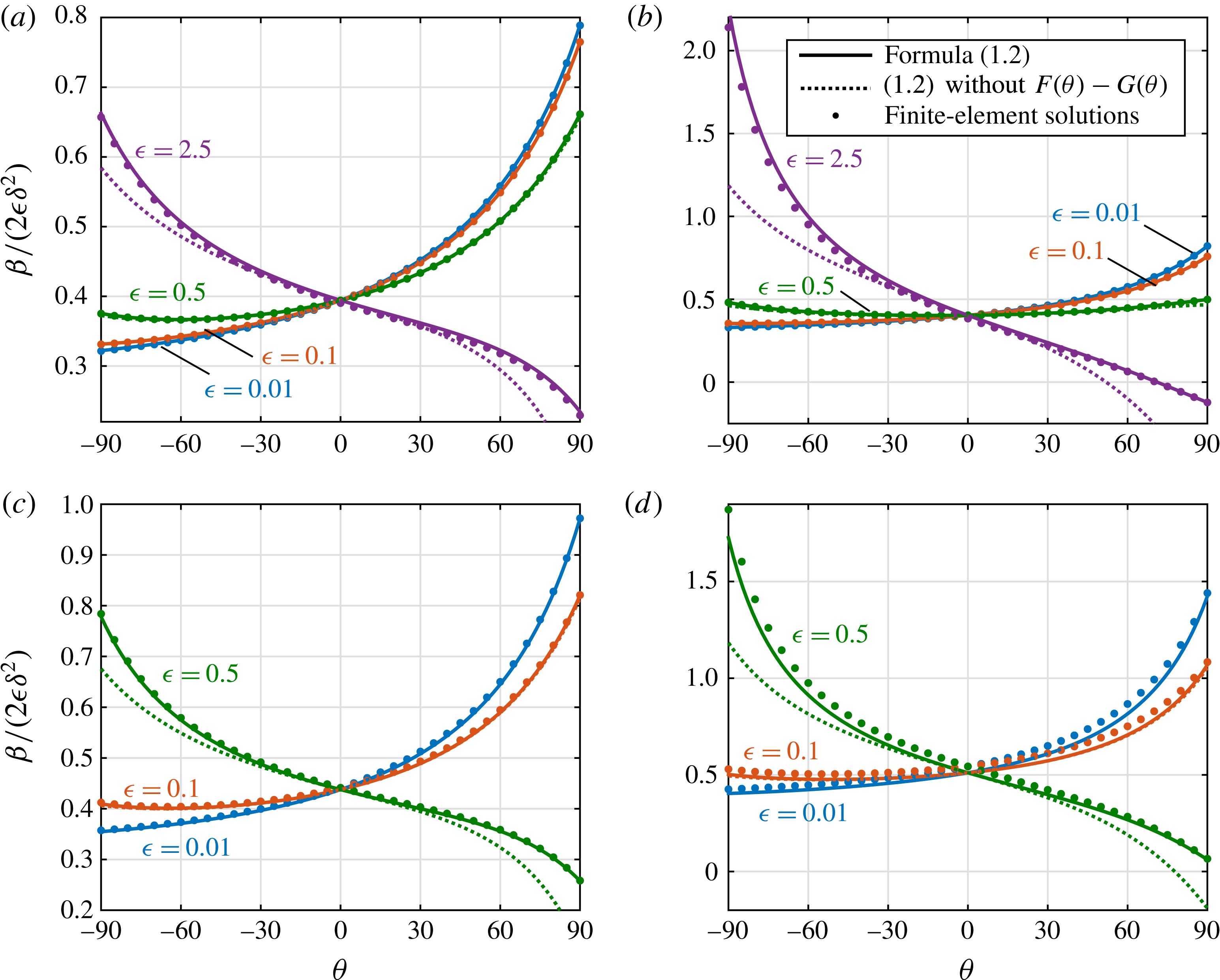
(a–d) Normalised slip length against protrusion angle (degrees) for slip fractions
 $\unicode[STIX]{x1D6FF}=0.1,\,0.25,\,0.5,\,0.75$
, respectively, and various aspect ratios
 $\unicode[STIX]{x1D716}$
. Solid lines are the full asymptotic solution (1.2); dotted lines are (1.2) with
 $F$
and
 $G$
neglected; dots are finite-element solutions.

The quantity
 $Q^{\prime }$
can be roughly interpreted as the change in flow rate due to the change in cross-sectional shape and area due to meniscus protrusion, i.e. a generalisation of
 $Q_{2}^{(1)}$
in Sbragaglia & Prosperetti (Reference Sbragaglia and Prosperetti2007) to arbitrary
 $\unicode[STIX]{x1D703}$
. From (5.6), we see that
 $Q^{\prime }=O(\unicode[STIX]{x1D716}^{2})$
, thus its contribution is necessary to compute
 $\unicode[STIX]{x1D6FD}$
beyond leading order in
 $\unicode[STIX]{x1D716}$
. This differs greatly from the case of a flat meniscus, where
 $Q^{\prime }\equiv 0$
and (1.2) reduces to
 $\unicode[STIX]{x1D6FD}=\unicode[STIX]{x1D716}\unicode[STIX]{x1D706}$
to all orders in
 $\unicode[STIX]{x1D716}$
(Hodes et al.
Reference Hodes, Kirk, Karamanis and MacLachlan2017).
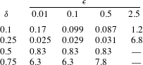
Maximum relative error (%) of
 $\unicode[STIX]{x1D6FD}/(2\unicode[STIX]{x1D716}\unicode[STIX]{x1D6FF}^{2})$
over
 $-\unicode[STIX]{x03C0}/2\leqslant \unicode[STIX]{x1D703}\leqslant \unicode[STIX]{x03C0}/2$
, between formula (1.2) and the numerical solution. For
 $\unicode[STIX]{x1D716}=2.5$
,
 $\unicode[STIX]{x1D6FF}=0.5,\,0.75$
see figure 3.

Two distinct asymptotic approximations,
 $\unicode[STIX]{x1D716}\ll 1$
and
 $\unicode[STIX]{x1D6FF}\ll 1$
, were made in order to derive (1.2). All algebraic orders in
 $\unicode[STIX]{x1D716}$
were accounted for before the dilute limit
 $\unicode[STIX]{x1D6FF}\ll 1$
was taken, but only up to
 $O(\unicode[STIX]{x1D6FF}^{5})$
, and thus the accuracy is limited by that of the
 $\unicode[STIX]{x1D6FF}$
-expansion. This is apparent when compared against finite-element computations of the full problem in the literature. Figure 2 compares
 $\unicode[STIX]{x1D6FD}/(2\unicode[STIX]{x1D716}\unicode[STIX]{x1D6FF}^{2})$
using formula (1.2) for ridges on one wall with results using PDEToolbox in Matlab (see Karamanis et al.
Reference Karamanis, Hodes, Kirk and Papageorgiou2017), for the same parameters as Teo & Khoo (Reference Teo and Khoo2010). The accuracy is uniform for the whole range of
 $\unicode[STIX]{x1D703}\in [-\unicode[STIX]{x03C0}/2,\unicode[STIX]{x03C0}/2]$
, and the maximum relative errors are shown in table 1. The accuracy in
 $\unicode[STIX]{x1D716}$
is remarkable; a negligible change is seen up to
 $\unicode[STIX]{x1D716}=0.5$
, when the channel height equals the period. Even more remarkable is that the error is still only
 $2\,\%{-}6\,\%$
up to
 $\unicode[STIX]{x1D716}=2.5$
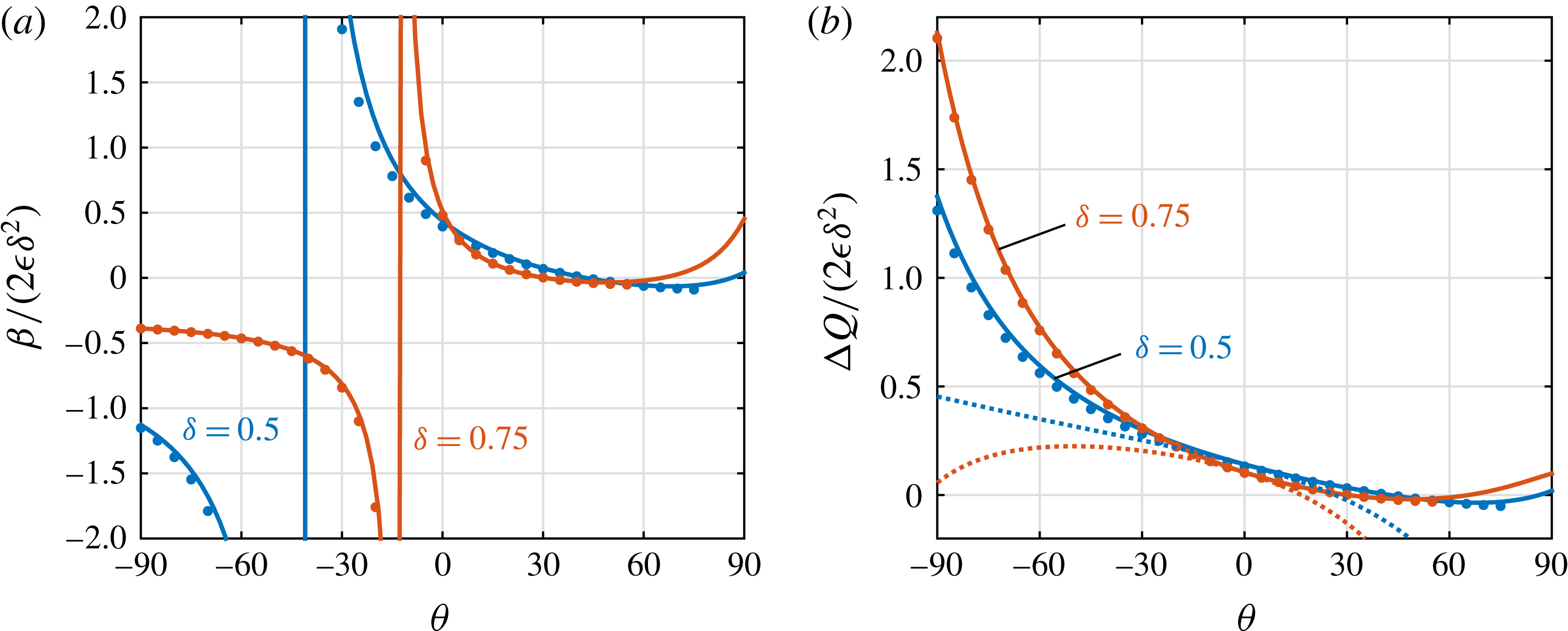
, when the height is five times smaller than the period. For this case, at slip fractions
 $\unicode[STIX]{x1D6FF}=0.5,\,0.75$
, the height is low enough for the slip length to become negative, which the asymptotics capture excellently, and for the meniscus to make contact with the upper wall; this occurs at
 $\unicode[STIX]{x1D703}=77^{\circ },56^{\circ }$
for
 $\unicode[STIX]{x1D6FF}=0.5,0.75$
, see figure 3. However, for these parameters, the slip length becomes singular for sufficient downward protrusion
 $(\unicode[STIX]{x1D703}<0)$
, due to a breakdown of the slip length definition (5.1), which rearranged is
 $\unicode[STIX]{x1D6FD}=1/(4/3-2Q)-1$
. This is singular when
 $Q=2/3$
, the flow rate for complete slip, i.e.
 $\unicode[STIX]{x2202}w/\unicode[STIX]{x2202}y=0$
on
 $y=0$
. For flow rates above
 $2/3$
, the enhancement due to the increase in area is greater than even complete slip, and
 $\unicode[STIX]{x1D6FD}$
loses its physical interpretation. This was not seen by Teo & Khoo (Reference Teo and Khoo2010) or Sbragaglia & Prosperetti (Reference Sbragaglia and Prosperetti2007) as they seem to use a definition for
 $\unicode[STIX]{x1D6FD}$
that is only valid for small
 $\unicode[STIX]{x1D6FD}$
. If we directly consider the flow rate enhancement relative to no-slip Poiseuille flow,
 $\unicode[STIX]{x0394}Q=Q-1/6$
, there is no singularity – see figure 3(b) – and the maximum relative error of the asymptotics is
 $5\,\%{-}8\,\%$
.
Normalised slip length (a) and change in flow rate (b) against protrusion angle (degrees) for slip fractions
 $\unicode[STIX]{x1D6FF}=0.5,\,0.75$
and at
 $\unicode[STIX]{x1D716}=2.5$
. Solid lines are the full asymptotic solution (1.2) and (5.6); dotted lines in (b) are (1.2) with
 $F$
and
 $G$
neglected; dots are finite-element solutions.

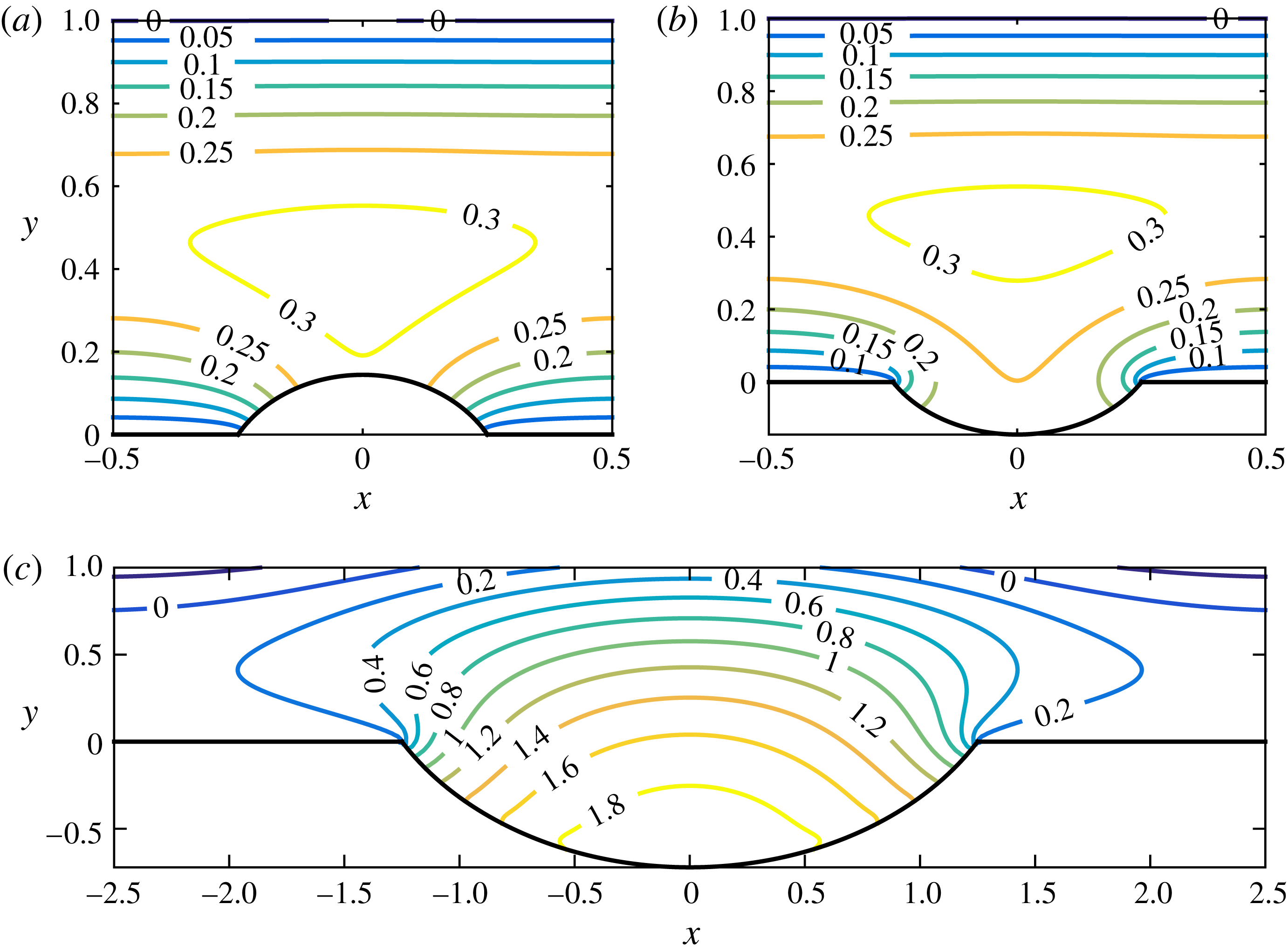
Asymptotic velocity field
 $w$
as given by (3.10) and (4.2). Slip fraction
 $\unicode[STIX]{x1D6FF}=0.5$
, protrusion angles
 $\unicode[STIX]{x1D703}=\pm 60^{\circ }$
. Square domain (
 $\unicode[STIX]{x1D716}=0.5$
) with
 $\unicode[STIX]{x1D703}=+60^{\circ }$
in (a) and
 $\unicode[STIX]{x1D703}=-60^{\circ }$
in (b); and
 $\unicode[STIX]{x1D716}=2.5$
with
 $\unicode[STIX]{x1D703}=-60^{\circ }$
in (c).

Further simplifications of the formula (1.2) are possible, but the accuracy can be greatly affected with little analytical gain. For example, if the
 $F(\unicode[STIX]{x1D703})$
and
 $G(\unicode[STIX]{x1D703})$
terms are neglected in (1.2), the formula is simpler but the accuracy for large angles is much worse – see dotted lines in figures 2 and 3. Other simplifications, such as using the lower-order approximations
 ${\hat{h}}_{0}(z)$
and
 $\hat{\unicode[STIX]{x1D706}}_{0}$
in (5.5), or expanding fractional terms, are even less accurate still, thus we do not include them here.
5.1 Asymptotic velocity field
Since the slip length is an integrated quantity of the flow, it is reasonable to question if the asymptotic velocity field itself is reliable. In fact (see figure 4), we find that the average error in the velocity is similar to that of the corresponding slip length, except for the large value
 $\unicode[STIX]{x1D716}=2.5$
. The asymptotic solution captures the behaviour near the ridge and meniscus well, by construction, but deviates most at the top of the channel – see the deviation up to
 $\pm 0.2$
from no-slip at
 $y=1$
in figure 4(c). This error does not appear in the slip length as it cancels to some extent after integration.
Acknowledgements
This work was supported by an EPSRC Doctoral Scholarship and Doctoral Prize Fellowship. The author is grateful to D. Crowdy for many helpful discussions and the inspiration for § 4, and to G. Karamanis for the finite-element data.
Supplementary material
Supplementary material is available at https://doi.org/10.1017/jfm.2018.73.