1. Introduction
Thermoacoustic oscillations of a confined premixed flame involve the interaction of acoustics and combustion. In order to model these oscillations in a numerically tractable way, it is usually necessary to use a low-order model for the flame. This reduced order model allows the system’s stability to be investigated and gives insights into the underlying mechanisms without resorting to full CFD (Dowling Reference Dowling1999; Schuller, Durox & Candel Reference Schuller, Durox and Candel2003; Lieuwen Reference Lieuwen2012).
In thermoacoustic systems, nonlinear relationships between velocity, pressure and heat release can be caused by gas dynamics, combustion and damping. The gas dynamics become nonlinear only when the acoustic Mach number is large (Chu Reference Chu1963; Culick Reference Culick1971; Yang, Kim & Culick Reference Yang, Kim and Culick1990). In most applications of practical interest today, such as gas turbine engines and laboratory experiments, the acoustic Mach number is small enough for nonlinear gas dynamics to be neglected. Solid and liquid rocket motors, however, have sufficiently high energy densities that the gas dynamics can become nonlinear. For these applications, any linear model of the acoustics, including that in this paper, will be an approximation. This paper focuses on nonlinear combustion. Nonlinear damping has been investigated by Heckl (Reference Heckl1990) and Matveev (Reference Matveev2003). It is influential but is not the subject of this paper.
A widely-used frequency domain approach is to measure or calculate the flame describing function (FDF), which approximates the nonlinear unsteady heat release response to finite-amplitude harmonic velocity or equivalence ratio fluctuations. In the linear limit, the FDF reduces to the flame transfer function (FTF), for which analytical expressions can be derived for some flames (Schuller et al. Reference Schuller, Durox and Candel2003; Preetham et al. Reference Santosh and Lieuwen2008; Shreekrishna & Lieuwen Reference Shreekrishna and Lieuwen2010). In a nonlinear framework, the FDF can be coupled with a model for the acoustics, and can predict the stability of a thermoacoustic system, as well as the frequency and amplitude of steady-state harmonic oscillations (Dowling Reference Dowling1997; Noiray et al. Reference Noiray, Durox, Schuller and Candel2008). However, it is restrictive to assume that the velocity fluctuations are harmonic. This precludes non-harmonic periodic oscillations, as well as more complex dynamical behaviour such as period-2, quasiperiodic and chaotic oscillations, which are common in thermoacoustics (Subramanian et al. Reference Subramanian, Mariappan, Sujith and Wahi2010; Gotoda et al. Reference Gotoda, Nikimoto, Miyano and Tachibana2011; Kabiraj & Sujith Reference Kabiraj and Sujith2012; Kabiraj, Sujith & Wahi Reference Kabiraj, Sujith and Wahi2012b ; Gotoda et al. Reference Gotoda, Shinoda, Kobayashi, Okuno and Tachibana2014).
On the other hand, time domain simulations do not make any a priori assumptions about the form of the acoustic fluctuations. These have been used successfully by Kashinath, Waugh & Juniper (Reference Kashinath, Waugh and Juniper2014) and Waugh, Kashinath & Juniper (Reference Waugh, Kashinath and Juniper2014) to simulate the nonlinear behaviour of thermoacoustic systems by time integration and continuation of limit cycles. These simulations qualitatively reproduce the elaborate dynamical behaviour found experimentally. So far, only a simplistic acoustic configuration has been considered in such studies: a duct with uniform cross-sectional area and no temperature variation across the flame. In this paper we present a general method to evaluate the acoustic response of an axisymmetric resonator containing, for example, area changes and temperature variations, and how to couple it with a kinematic flame model based on the
 $G$
-equation both in the frequency and time domains. This allows the methods of Kashinath et al. (Reference Kashinath, Waugh and Juniper2014) and Waugh et al. (Reference Waugh, Kashinath and Juniper2014) to be generalized to practical thermoacoustic systems.
There are several ways to formulate a linear acoustic model for a thermoacoustic analysis. Three common methods are (i) a Galerkin discretization (Zinn & Lores Reference Zinn and Lores1971; Culick Reference Culick1976a ,Reference Culick b ); (ii) a Green’s function approach (Heckl & Howe Reference Heckl and Howe2007), which may subsequently be used in a modal expansion (Schuermans Reference Schuermans2003); and (iii) a wave-based approach (Lang, Poinsot & Candel Reference Lang, Poinsot and Candel1987; Heckl Reference Heckl1988). In any acoustic modelling method, it is useful to write the resulting model in state-space form (to be defined in § 3.2.1) because this allows powerful techniques from dynamics and control to be used. These include, for example, stability analysis of the coupled thermoacoustic system, analysis of its transient growth characteristics, and the design of feedback control to eliminate oscillations. For the Galerkin discretization and the Green’s function approach, methods to describe the resulting systems in state-space form have been developed. For a Galerkin discretization, a state-space description follows quite naturally from the Galerkin modes, and for a Green’s function approach, a state-space description can be generated by performing a modal expansion (Schuermans Reference Schuermans2003). For the wave-based approach, however, it is less straightforward to describe the resulting system in state-space form. This is largely due to time delay terms, which make the system infinite-dimensional, and which are not amenable to a state-space description in a straightforward way. A possibility is to approximate time delays with, e.g. Padé approximations, as in Bothien et al. (Reference Bothien, Moeck, Lacarelle and Paschereit2007), or to make use of a state vector with memory, i.e. a state vector that includes the acoustic states at previous times, as in Mangesius & Polifke (Reference Mangesius and Polifke2011). Here, we develop an alternative approach that allows us to cast the frequency response of the system in state-space form.
In § 2 we discuss the combustion and flow models. Further details on these models and methods used to numerically integrate them can be found in Peng et al. (Reference Peng, Merriman, Osher, Zhao and Kang1999), Sethian (Reference Sethian1999) and Kashinath et al. (Reference Kashinath, Waugh and Juniper2014). In § 3 the acoustic network modelling is described, and we describe our state-space formulation. In § 4 a numerically evaluated FDF is shown, and we perform a stability analysis of our thermoacoustic system by means of the harmonic balance technique. The same thermoacoustic configuration is investigated in § 5 in the time domain with two different techniques. In § 6 bifurcation diagrams are shown, and we discuss the analogies and differences between the results predicted by the various methods. Finally in § 7 we focus on the nonlinear dynamical behaviour we observe and we compare it with analogous studies.
2. Flame model
In this section we describe the model for the flame dynamics and unsteady heat release fluctuations. It is based on the well-known
 $G$
-equation model (Markstein Reference Markstein1964), accounting for curvature effects on the flame speed. We also introduce the flow field model, which is based on previous studies (Kashinath, Hemchandra & Juniper Reference Kashinath, Hemchandra and Juniper2013b
).
2.1. Flame and flow field model
The
 $G$
-equation model (Markstein Reference Markstein1964) provides a low-cost method that enables premixed flames dynamics and heat release to be described qualitatively. The
 $G$
-field is a smooth scalar field whose isocontour
 $G=0$
identifies the flame surface. This contour separates reactants (
 $G<0$
) from products (
 $G>0$
) (see figure 5
b).
The velocity of the flame surface is the sum of the underlying flow velocity
 $\boldsymbol{U}$
and the burning velocity,
 $s_{L}\hat{\boldsymbol{n}}$
, where
 $\hat{\boldsymbol{n}}$
is the unit vector normal to the flame, defined by
 $$\begin{eqnarray}\hat{\boldsymbol{n}}\equiv -\frac{\boldsymbol{{\rm\nabla}}G}{\left|\boldsymbol{{\rm\nabla}}G\right|},\end{eqnarray}$$
and points towards the unburnt gas. By taking the material derivative of the
 $G=0$
level set, we arrive at the transport equation
 $$\begin{eqnarray}\frac{\partial G}{\partial t}+\boldsymbol{U}\boldsymbol{\cdot }\boldsymbol{{\rm\nabla}}G=s_{L}\left|\boldsymbol{{\rm\nabla}}G\right|,\end{eqnarray}$$
which is known as the
 $G$
-equation. Equation (2.2) has been deeply investigated and used in thermoacoustics both in the linear limit, to determine FTFs (Schuller et al.
Reference Schuller, Durox and Candel2003; Preetham et al.
Reference Santosh and Lieuwen2008; Shreekrishna & Lieuwen Reference Shreekrishna and Lieuwen2010), and in the fully nonlinear regime, to simulate forced and self-excited oscillations (Kashinath et al.
Reference Kashinath, Waugh and Juniper2014). The local flame speed
 $s_{L}$
is a function of the equivalence ratio
 ${\it\phi}$
, the type of fuel, the flame curvature and, for turbulent flames, the turbulent intensity. In this paper, we consider laminar, fully premixed flames. Therefore, the equivalence ratio is constant and uniform but the flame speed depends on local curvature effects (Markstein Reference Markstein1964; Creta & Matalon Reference Creta and Matalon2011):
 $$\begin{eqnarray}s_{L}=s_{L}^{0}\left(1-\mathscr{L}{\it\kappa}\right).\end{eqnarray}$$
Here
 $s_{L}^{0}$
is the speed of a laminar, flat flame sheet,
 ${\it\kappa}\equiv \boldsymbol{{\rm\nabla}}\boldsymbol{\cdot }\hat{\boldsymbol{n}}$
is the local flame curvature and
 $\mathscr{L}$
is the Markstein length.
In this study we consider an axisymmetric geometry (§ 3.3) using a cylindrical coordinate system
 $(r,{\it\theta},x)$
. The velocity field
 $\boldsymbol{U}=(u_{r},u_{{\it\theta}}=0,u_{x})$
is decomposed into mean (
 $\overline{\boldsymbol{U}}$
) and fluctuating (
 $\boldsymbol{U}^{\prime }$
) components. The mean flow is assumed to be only a function of
 $x$
. For the perturbation, the axial velocity (forced or self-excited) is imposed at the burner every instant and the radial velocity is found by continuity:
 $$\begin{eqnarray}\frac{1}{r}\frac{\partial \left(u_{r}^{\prime }r\right)}{\partial r}+\frac{\partial u_{x}^{\prime }}{\partial x}=0.\end{eqnarray}$$
DNS calculations show that these perturbations advect axially at a frequency-dependent speed that is slower than the mean flow (Kashinath et al.
Reference Kashinath, Hemchandra and Juniper2013b
). We do not know the acoustic frequencies a priori, so we fix this speed at
 $0.833\overline{u}_{x}$
, which is the largest value observed by Kashinath et al. (Reference Kashinath, Hemchandra and Juniper2013b
).
Substituting the flow field and flame speed expression (2.3) into (2.2), and introducing the non-dimensional parameters
 $$\begin{eqnarray}\frac{x}{L_{f}}\rightarrow x\quad \frac{r}{R}\rightarrow r\quad \frac{u_{x}}{\overline{u}_{x}}\rightarrow u_{x}\quad \frac{u_{r}}{\overline{u}_{x}}\rightarrow u_{r}\quad \frac{t\,\overline{u}_{x}}{L_{f}}\rightarrow t,\end{eqnarray}$$
we obtain
 $$\begin{eqnarray}\frac{\partial G}{\partial t}+{\it\beta}u_{r}^{\prime }\frac{\partial G}{\partial r}+\left(1+u_{x}^{\prime }\right)\frac{\partial G}{\partial x}=\frac{s_{L}^{0}}{\overline{u}_{x}}\left(1-\mathscr{M}{\it\kappa}\right)\sqrt{\left({\it\beta}\frac{\partial G}{\partial r}\right)^{2}+\left(\frac{\partial G}{\partial x}\right)^{2}},\end{eqnarray}$$
where
 $L_{f}$
is the flame height,
 $R$
is the burner radius,
 ${\it\beta}\equiv L_{f}/R$
is the flame aspect ratio and
 $\mathscr{M}$
is the ratio between the Markstein length and the flame height.
The nonlinear PDE (2.6) summarises the combustion model adopted. It is integrated numerically using LSGEN2D, a level set solver originally developed by Hemchandra (Reference Hemchandra2009) and then developed by Kashinath et al. (Reference Kashinath, Waugh and Juniper2014), Waugh et al. (Reference Waugh, Kashinath and Juniper2014) and in the current study. The numerical method used to evolve the
 $G$
-field is the narrow band level set technique, as described by Peng et al. (Reference Peng, Merriman, Osher, Zhao and Kang1999) and Sethian (Reference Sethian1999).
3. Acoustics
In this section we describe the wave-based acoustic model and generate a state-space acoustic model from it. We start with a simple case: a flame in a one-dimensional duct open at both ends. This shows the important features of the wave-based method and highlights the difficulties in formulating its state-space description. Then we introduce the geometry considered in the remainder of the paper and generate its acoustic network model.
3.1. Wave-based modelling approach
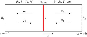
Figure 1 shows the first model: an acoustically compact flame inside an open-ended duct. The mean flow, if non-zero, is from left to right. There is a temperature jump across the flame, which causes the sound speed to increase from
 $\bar{c}_{1}$
to
 $\bar{c}_{2}$
. A perturbation in the heat release,
 $q^{\prime }(t)$
, generates outward-travelling waves that propagate both upstream (
 ${\it\alpha}_{1}$
) and downstream (
 ${\it\alpha}_{2}$
). These waves partially reflect at the upstream/downstream ends of the duct. The reflection coefficients are
 $R_{1}$
and
 $R_{2}$
, and the reflected waves are
 ${\it\beta}_{1}$
and
 ${\it\beta}_{2}$
. The flame is at
 $x=0$
, so
 $x\in [-l_{1},0)$
is upstream of the flame and
 $x\in (0,l_{2}]$
is downstream of the flame.
Wave approach in a simple duct geometry.
 ${\it\alpha}_{1}$
and
 ${\it\alpha}_{2}$
are the waves radiated from the heat source towards the boundaries in the upstream and downstream regions respectively. Here
 ${\it\beta}_{1}$
and
 ${\it\beta}_{2}$
are the waves reflected by the boundaries.

We solve the wave equation in each of the two regions shown in figure 1. Upstream of the flame, the acoustic pressure and velocity perturbations can be written in terms of the upstream- and downstream-travelling waves,
 ${\it\alpha}_{1}$
and
 ${\it\beta}_{1}$
:
 $$\begin{eqnarray}\displaystyle & \displaystyle p_{1}^{\prime }(x,t)={\it\alpha}_{1}\left(t+\frac{x}{\bar{c}_{1}-\bar{u}_{1}}\right)+{\it\beta}_{1}\left(t-\frac{x}{\bar{c}_{1}+\bar{u}_{1}}\right) & \displaystyle\end{eqnarray}$$
 $$\begin{eqnarray}\displaystyle & \displaystyle u_{1}^{\prime }(x,t)=\frac{1}{\bar{{\it\rho}}_{1}\bar{c}_{1}}\left[-{\it\alpha}_{1}\left(t+\frac{x}{\bar{c}_{1}-\bar{u}_{1}}\right)+{\it\beta}_{1}\left(t-\frac{x}{\bar{c}_{1}+\bar{u}_{1}}\right)\right]. & \displaystyle\end{eqnarray}$$
 $\text{}_{x}$
for the axial velocity. These equations are supplemented by boundary conditions at each end of the duct, which provide a relationship between the outward-travelling waves,
 ${\it\alpha}_{1}(t)$
and
 ${\it\alpha}_{2}(t)$
, and the inward-travelling waves,
 ${\it\beta}_{1}(t)$
and
 ${\it\beta}_{2}(t)$
:
 $$\begin{eqnarray}\displaystyle & \displaystyle {\it\beta}_{1}\left(t+\frac{l_{1}}{\bar{c}_{1}+\bar{u}_{1}}\right)=R_{1}{\it\alpha}_{1}\left(t-\frac{l_{1}}{\bar{c}_{1}-\bar{u}_{1}}\right) & \displaystyle\end{eqnarray}$$
 $$\begin{eqnarray}\displaystyle & \displaystyle {\it\beta}_{2}\left(t+\frac{l_{2}}{\bar{c}_{2}-\bar{u}_{2}}\right)=R_{2}{\it\alpha}_{2}\left(t-\frac{l_{2}}{\bar{c}_{2}+\bar{u}_{2}}\right). & \displaystyle\end{eqnarray}$$
We need to relate the upstream and downstream flow to the heat release rate. This is achieved by considering the mass, momentum and energy balances across the flame. By considering linearized disturbances of the momentum and energy equations and substituting in the travelling-wave solutions (3.1) with boundary conditions (3.2), we obtain the equations governing the time evolution of the outward-travelling waves
 $$\begin{eqnarray}\unicode[STIX]{x1D653}\left[\begin{array}{@{}c@{}}{\it\alpha}_{1}(t)\\ {\it\alpha}_{2}(t)\end{array}\right]=\unicode[STIX]{x1D654}\left[\begin{array}{@{}c@{}}R_{1}{\it\alpha}_{1}(t-{\it\tau}_{1})\\ R_{2}{\it\alpha}_{2}(t-{\it\tau}_{2})\end{array}\right]+\left[\begin{array}{@{}c@{}}0\\ 1\end{array}\right]\frac{q^{\prime }(t)}{\bar{c}_{1}},\end{eqnarray}$$
where
 ${\it\tau}_{1}=2l_{1}\bar{c}_{1}/(\bar{c}_{1}^{2}-\bar{u}_{1}^{2})$
,
 ${\it\tau}_{2}=2l_{2}\bar{c}_{2}/(\bar{c}_{2}^{2}-\bar{u}_{2}^{2})$
, and
 $\unicode[STIX]{x1D653}$
and
 $\unicode[STIX]{x1D654}$
are
 $2\times 2$
matrices and are functions of the mean flow properties only. These matrices are a more general form of the matrices contained in Dowling (Reference Dowling1997).
In order to demonstrate the wave-based approach, we consider the zero mean flow case. This simplifies the analysis significantly, whilst still retaining the most important features. Taking the Laplace transform of (3.3) for no mean flow, and assuming that the reflection coefficients are frequency-independent, we find
 $$\begin{eqnarray}\left[\begin{array}{@{}cc@{}}1+R_{1}\text{e}^{-s{\it\tau}_{1}} & -1-R_{2}\text{e}^{-s{\it\tau}_{2}}\\ 1-R_{1}\text{e}^{-s{\it\tau}_{1}} & \displaystyle \frac{\bar{c}_{2}}{\bar{c}_{1}}(1-R_{2}\text{e}^{-s{\it\tau}_{2}})\end{array}\right]\left[\begin{array}{@{}c@{}}{\it\alpha}_{1}(s)\\ {\it\alpha}_{2}(s)\end{array}\right]=\left[\begin{array}{@{}c@{}}0\\ \displaystyle \frac{{\it\gamma}-1}{\bar{c}_{1}}\end{array}\right]q^{\prime }(s),\end{eqnarray}$$
where
 $s\equiv {\it\sigma}+\text{i}{\it\omega}$
is the Laplace variable and
 ${\it\sigma}$
the growth rate. The modes are now given by those values of
 $s$
for which the determinant
 ${\it\Omega}(s)$
of the matrix in (3.4) vanishes. This gives us the relation
 $$\begin{eqnarray}{\it\Omega}(s)\equiv \left(1+\frac{\bar{c}_{2}}{\bar{c}_{1}}\right)\left(1-R_{1}R_{2}\text{e}^{-s({\it\tau}_{1}+{\it\tau}_{2})}\right)+\left(1-\frac{\bar{c}_{2}}{\bar{c}_{1}}\right)\left(R_{2}\text{e}^{-s{\it\tau}_{2}}-R_{1}\text{e}^{-s{\it\tau}_{1}}\right)=0,\end{eqnarray}$$
which makes clear the influence of the ratio of the speeds of sound,
 $\bar{c}_{2}/\bar{c}_{1}$
. When
 $\bar{c}_{2}/\bar{c}_{1}=1$
(i.e. no temperature change across the flame) the modes are equispaced and given simply by
 $$\begin{eqnarray}R_{1}R_{2}\text{e}^{-s({\it\tau}_{1}+{\it\tau}_{2})}=1.\end{eqnarray}$$
When
 $\bar{c}_{2}/\bar{c}_{1}\neq 1$
there is an extra term in (3.5) and the modes are no longer equispaced.
Solving (3.4) for the waves
 ${\it\alpha}_{1}(s)$
and
 ${\it\alpha}_{2}(s)$
, and substituting these into the expressions (3.1) for the pressure and velocity, we find for the upstream region that
 $$\begin{eqnarray}\displaystyle & \displaystyle \frac{p_{1}^{\prime }(x_{1},s)}{q^{\prime }(s)}=\frac{{\it\gamma}-1}{\bar{c}_{1}}\frac{[1+R_{2}\text{e}^{-s{\it\tau}_{2}}]\left[1+R_{1}\text{e}^{-s\left({\it\tau}_{1}-(2x_{1}/\bar{c}_{1})\right)}\right]}{{\it\Omega}(s)}\text{e}^{-s(x_{1}/\bar{c}_{1})} & \displaystyle\end{eqnarray}$$
 $$\begin{eqnarray}\displaystyle & \displaystyle \frac{u_{1}^{\prime }(x_{1},s)}{q^{\prime }(s)}=\frac{{\it\gamma}-1}{2\bar{{\it\rho}}_{1}\bar{c}_{1}^{2}}\frac{[1+R_{2}\text{e}^{-s{\it\tau}_{2}}]\left[-1+R_{1}\text{e}^{-s\left({\it\tau}_{1}-(2x_{1}/\bar{c}_{1})\right)}\right]}{{\it\Omega}(s)}\text{e}^{-s(x_{1}/\bar{c}_{1})}. & \displaystyle\end{eqnarray}$$
 $\text{e}^{-s{\it\tau}}$
, and it is therefore not possible to cast them directly in state-space form. Time delays can be approximated by Padé approximations in order to make them amenable to state-space descriptions (Bothien et al.
Reference Bothien, Moeck, Lacarelle and Paschereit2007). Alternatively, state vectors that include the acoustic states at previous times can be used (Mangesius & Polifke Reference Mangesius and Polifke2011). However, we have opted for a different approach to the state-space formulation, which is presented in the next section.
3.2. Finding a state-space model
Having outlined the most important features of the wave-based model, we now obtain its state-space description using knowledge of its acoustic modes and frequency response. Rather than discretize the system using an expansion such as Fourier modes, we discretize the system by finding its eigenvalues directly. This involves finding the roots,
 ${\it\lambda}_{k}\equiv {\it\sigma}_{k}+\text{i}{\it\omega}_{k}$
, of
 ${\it\Omega}(s)$
introduced in (3.5). This is achieved using Newton–Raphson iteration in the complex plane. We also require the frequency response function, which is found by setting
 $s=\text{i}{\it\omega}$
in (3.7). This information can be retrieved without invoking Padé approximations. We then approximate the frequency response with a state-space model, as described in the next section.
3.2.1. Calculating the state-space matrices
We want to be able to write the acoustic model described in § 3 in state-space form:
 $$\begin{eqnarray}\displaystyle & \dot{\boldsymbol{x}}(t)=\unicode[STIX]{x1D63C}\,\boldsymbol{x}(t)+\unicode[STIX]{x1D63D}\,q^{\prime }(t) & \displaystyle\end{eqnarray}$$
 $$\begin{eqnarray}\displaystyle & y^{\prime }(t)=\unicode[STIX]{x1D63E}\,\boldsymbol{x}(t)+\unicode[STIX]{x1D63F}\,q^{\prime }(t), & \displaystyle\end{eqnarray}$$
 $\boldsymbol{x}$
is the state vector,
 $q^{\prime }$
is an input and
 $y^{\prime }$
is some output of interest. In our case the input signal is the fluctuating heat release, and the outputs of interest are velocity and pressure fluctuations. Taking Laplace transforms of (3.8) and rearranging, we arrive at the transfer function
 $$\begin{eqnarray}G(s)\equiv \frac{y^{\prime }(s)}{q^{\prime }(s)}=\unicode[STIX]{x1D63E}\left(s\unicode[STIX]{x1D644}-\unicode[STIX]{x1D63C}\right)^{-1}\unicode[STIX]{x1D63D}+\unicode[STIX]{x1D63F},\end{eqnarray}$$
where
 $\unicode[STIX]{x1D644}$
is the identity matrix.
A state-space realization is not unique. There are many state-space realizations that give the same transfer function. The realization that is convenient for our purposes is a modal form, where the
 $\unicode[STIX]{x1D63C}$
matrix is written as a diagonal matrix with its eigenvalues on its diagonal. For this realization, the term
 $(s\unicode[STIX]{x1D644}-\unicode[STIX]{x1D63C})^{-1}$
can be written simply as
 $$\begin{eqnarray}(s\unicode[STIX]{x1D644}-\unicode[STIX]{x1D63C})^{-1}=\left[\begin{array}{@{}ccc@{}}s-{\it\lambda}_{1} & \cdots \, & 0\\ \vdots & \ddots & \vdots \\ 0 & \cdots \, & s-{\it\lambda}_{n}\end{array}\right]^{-1}=\left[\begin{array}{@{}ccc@{}}\displaystyle \frac{1}{s-{\it\lambda}_{1}} & \cdots \, & 0\\ \vdots & \ddots & \vdots \\ 0 & \cdots \, & \displaystyle \frac{1}{s-{\it\lambda}_{n}}\end{array}\right],\end{eqnarray}$$
and the transfer function,
 $G(s)$
, becomes
 $$\begin{eqnarray}G(s)=\mathop{\sum }_{k=1}^{n}\frac{c_{k}b_{k}}{s-{\it\lambda}_{k}}=\mathop{\sum }_{k=1}^{n}\frac{{\it\theta}_{k}}{s-{\it\lambda}_{k}}.\end{eqnarray}$$
Here we have defined
 ${\it\theta}_{k}\equiv c_{k}b_{k}$
. This is for the single-input–single-output case, for which
 $\boldsymbol{B}$
is a column vector and
 $\boldsymbol{C}$
is a row vector, but is easily extended to the multi-input–multi-output case. If we evaluate the frequency response of
 $G(s)|_{s=\text{i}{\it\omega}}$
at the frequencies
 ${\it\omega}_{1},{\it\omega}_{2},\dots ,{\it\omega}_{p}$
, then
 $$\begin{eqnarray}\left[\begin{array}{@{}c@{}}G(\text{i}{\it\omega}_{1})\\ \vdots \\ G(\text{i}{\it\omega}_{p})\end{array}\right]=\left[\begin{array}{@{}ccc@{}}\left(\text{i}{\it\omega}_{1}-{\it\lambda}_{1}\right)^{-1} & \cdots \, & \left(\text{i}{\it\omega}_{1}-{\it\lambda}_{n}\right)^{-1}\\ \vdots & \ddots & \vdots \\ \left(\text{i}{\it\omega}_{p}-{\it\lambda}_{1}\right)^{-1} & \cdots \, & \left(\text{i}{\it\omega}_{p}-{\it\lambda}_{n}\right)^{-1}\end{array}\right]\left[\begin{array}{@{}c@{}}{\it\theta}_{1}\\ \vdots \\ {\it\theta}_{n}\end{array}\right],\end{eqnarray}$$
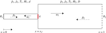
Acoustic network considered in this study. It is based on the experimental set-up described by Kabiraj & Sujith (Reference Kabiraj and Sujith2012). The flame position
 $x_{f}$
is the bifurcation parameter we will investigate. The flame, assumed to be acoustically compact, induces a mean temperature change and consequent mean flow properties variations. An area change models the blockage introduced by the burner holding the flame.

which we can solve for
 $\left[\begin{array}{@{}c@{}}{\it\theta}_{1}\cdots {\it\theta}_{n}\end{array}\right]^{\text{T}}$
. We need the frequency response at
 $p=n$
frequencies to make the matrix in (3.12) invertible. In practice, however, it is better to evaluate the frequency response at many more than
 $n$
frequencies,
 $p\gg n$
, and then solve (3.12) in the least squares sense. Note that we are free to choose any
 $c_{k}$
,
 $b_{k}$
, provided they satisfy
 $c_{k}b_{k}={\it\theta}_{k}$
.
A validation of the agreement between the original frequency response and the approximated state-space form has been given by Illingworth & Juniper (Reference Illingworth and Juniper2014): for an approximation order
 $n=23$
, the agreement is excellent at low frequencies, and slightly deteriorates at high frequencies. This is expected because the state-space model cuts off the contribution of modes with high frequencies.
3.3. Description of the low-order thermoacoustic network model
The analysis in § 3.1 was for a simple open-ended duct, which served to illustrate the wave-based modelling approach. We now describe the more complex acoustic network we investigate.
The acoustic network (figure 2) is based on the experimental rig of Kabiraj & Sujith (Reference Kabiraj and Sujith2012): a laminar flame attached to a tube (diameter
 $D=11~\text{mm}$
) inside an open–closed pipe of length
 $L=860~\text{mm}$
and diameter
 $D_{L}=25.6~\text{mm}$
. The acoustic network has a temperature jump across the flame and an area increase to emulate the blockage caused by the burner tube upstream of the flame. The area increase is treated as a discontinuity, and we use jump conditions dictated by mass and momentum conservation to solve for the flow after the area change. The temperature ratio is
 $T_{2}/T_{1}=2$
, and the mean flow speed is
 $\overline{u}=1.55~\text{m}~\text{s}^{-1}$
. A lean equivalence ratio regime is analysed, with
 ${\it\phi}=0.51$
. The laminar flame speed is assumed to be
 $s_{L}^{0}=0.25~\text{m}~\text{s}^{-1}$
and the Markstein length is fixed to
 $\mathscr{L}=0.6~\text{mm}$
. This leads to a steady flame having an aspect ratio
 ${\it\beta}\equiv L_{f}/R\approx 6$
. Damping effects are included by means of losses at boundaries; the closed inlet reflection coefficient is set to
 $R_{1}=1.0$
, and the outlet reflection coefficient is that of an unflanged cylindrical open end in the low-Mach-number limit (Eldredge & Dowling Reference Eldredge and Dowling2003):
 $$\begin{eqnarray}R_{2}=-(1+0.9M)\left(1-\frac{1}{2}\frac{{\it\omega}^{2}R^{2}}{c^{2}}\right).\end{eqnarray}$$
The non-dimensional flame position is
 $x_{f}\equiv l_{1}/L$
, where
 $L\equiv l_{1}+l_{2}$
is the length of the pipe. The acoustic time scale is defined by the acoustic Strouhal number
 $St_{2}\equiv {\it\omega}L/\bar{c}_{1}$
.
Although the acoustic configuration is simple, the frequency-dependence of the reflection coefficients makes it hard to analytically determine the acoustic transfer functions to heat release fluctuations. Therefore, we rely on numerical methods. We use LOTAN, which is a low-order thermoacoustic network model developed by Dowling & Stow (Reference Dowling and Stow2003) for the simulation of longitudinal and annular combustion systems. The low-order modelling approach is based on the fact that the main nonlinearity is in the combustion response to flow perturbations rather than in the acoustics (Chu Reference Chu1963; Culick Reference Culick1971). LOTAN has been verified experimentally against both a sector rig (Stow & Dowling Reference Stow and Dowling2001) and an atmospheric test rig (Stow & Dowling Reference Stow and Dowling2004). The combustion system is modelled as a series of interconnected modules. Longitudinal ducts, annular ducts, combustion zones and area changes are amongst the module types that can be modelled. The model decomposes the flow into a steady mean axial component and small perturbations. The perturbations throughout the combustor are related via wave propagation, in which acoustic, entropy and vorticity waves are all included. The flow conservation equations are used to track the evolution of these waves. The connecting modules are modelled as acoustically compact, meaning that their axial length is short in comparison to the acoustic wavelengths of interest. The acoustic boundary conditions at the inlet and outlet of the combustor are assumed to be known, and these can be prescribed as frequency-dependent functions. The flame is assumed to combust at one axial location, i.e. to be acoustically compact.
Although LOTAN is able to model quite complex acoustic geometries, the range of flame models currently available in LOTAN is relatively limited. We therefore use LOTAN in an unconventional way. We take full advantage of LOTAN’s advanced acoustic modelling capabilities by extracting the acoustic eigenfrequencies and the network frequency response. Then we cast it in state-space form as in § 3.2. We find that an approximation order
 $n=20$
is always sufficient to properly describe the frequency response with a state space. Finally, rather than coupling this with a flame model directly in LOTAN, we couple the extracted acoustic model with the
 $G$
-equation model described in § 2.1. By doing so, we are able to model the coupled dynamics of complex acoustics with a flame model which is also complex, and study the thermoacoustic system in the time domain.
3.4. Effect of temperature jump
Previous studies in the time domain (Kashinath et al. Reference Kashinath, Waugh and Juniper2014; Waugh et al. Reference Waugh, Kashinath and Juniper2014) have examined straight pipes with uniform acoustic mean properties and zero mean flow. The low-order thermoacoustic framework proposed here, however, includes a mean flow, temperature and cross-sectional area variations, and can therefore analyse more general configurations.
Varying the flame position in the acoustic network, we evaluate transfer functions
 $G_{x_{f}}(s)$
and fit them to state-space models as described in § 3.2.1. When the reflection coefficients are equal to
 $\pm 1$
, the acoustic response can be thought of as a Galerkin discretization onto a basis set formed by the orthogonal acoustic eigenmodes
 ${\it\psi}_{k}^{ac}$
:
 $$\begin{eqnarray}u^{\prime }(x,t)\approx \mathop{\sum }_{k=1}^{N}\hat{u} _{k}^{\prime }(t){\it\psi}_{k}^{ac}(x)\end{eqnarray}$$
evaluated at the flame position. Indeed,
 $[{\it\psi}_{1}^{ac}(x_{f}),\dots ,{\it\psi}_{N}^{ac}(x_{f})]=\boldsymbol{C}$
, where
 $\boldsymbol{C}$
is the state-space vector as in (3.8b
). Note that this analogy is not true in general, because the acoustic eigenvectors are non-orthogonal for non-trivial reflection coefficients (Nicoud et al.
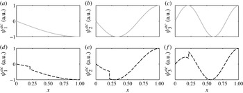
Reference Nicoud, Benoit, Sensiau and Poinsot2007). Figure 3 shows a comparison between the first three eigenmodes of an open–closed pipe with
 $R_{1}=1.0$
and
 $R_{2}=-1$
with and without a temperature jump. In the latter case, the Galerkin basis functions correspond to a Fourier expansion, i.e.
 ${\it\psi}_{k}^{ac}=\text{e}^{\text{i}kx}$
, which we find in the limit
 $T_{2}/T_{1}\rightarrow 1$
. In both cases, the thermoacoustic modes contain a discontinuity at the flame location, which is typically modelled with a Dirac delta in systems with no mean temperature effects. In networks with a temperature jump across the flame, the discontinuity naturally arises since it is present in all of the acoustic basis functions.
Acoustic velocity mode shapes evaluated with a Fourier–Galerkin basis (a–c), analogous to the limit
 $T_{2}/T_{1}\rightarrow 1$
, and LOTAN (d–f), with
 $T_{2}/T_{1}=2$
. In the former case the modes are continuous and correspond to the natural acoustic eigenmodes of the open–closed pipe, in the latter a discontinuity is located at the flame position because of a sudden change in the speed of sound.

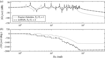
Thermoacoustic oscillation frequencies are often found to be close to the acoustic natural frequencies (Dowling & Stow Reference Dowling and Stow2003; Noiray et al. Reference Noiray, Durox, Schuller and Candel2008). This will be the case in our configuration, as we discuss in the next section. These acoustic eigenfrequencies change significantly when the mean temperature is non-uniform, as is shown in figure 4, and are no longer multiples of the fundamental frequency (see (3.5)). This reduces coupling between the modes, which will be discussed later.
Transfer functions of velocity fluctuations with respect to heat release fluctuations for a straight open–closed duct with a flame positioned at
 $x_{f}=0.213$
. (a) Fourier–Galerkin (solid line) state space, as in Kashinath, Hemchandra & Juniper (Reference Kashinath, Hemchandra and Juniper2013a
): the poles’ locations remain at the natural frequencies of the open–closed pipe. (b) LOTAN (dot-dashed line) state space, with
 $T_{2}/T_{1}=2$
: the position of the poles is shifted because the mean acoustic properties vary with
 $T_{2}/T_{1}$
.

4. Nonlinear analysis in the frequency domain
In this section we analyse thermoacoustic oscillations in the frequency domain. This is accomplished by numerically evaluating a FDF to inlet harmonic velocity fluctuations. The FDF is coupled in a feedback loop with acoustic transfer functions.
4.1. Flame describing function
In most thermoacoustic systems, the flame is the main source of nonlinearity (Chu Reference Chu1963; Culick Reference Culick1971). The FDF method exploits this characteristic; it approximates the flame’s nonlinear response to an imposed input signal. We denote with
 $\mathscr{F}(\mathit{St},A)$
the FDF of a sinusoidal input with angular frequency
 $2{\rm\pi}\mathit{St}$
and amplitude
 $A$
. When we close the FDF in a feedback loop with an acoustic transfer function
 $G(\mathit{St})$
, we can predict the frequency, amplitude and stability of limit cycles via the harmonic balance (or describing function method) (Khalil Reference Khalil2001).
We numerically construct an FDF by harmonically forcing the axial flow at the flame inlet at various frequencies
 $f={\it\omega}/(2{\rm\pi})$
and amplitudes. Solving continuity and advection equations, the perturbation flow reads
 $$\begin{eqnarray}u^{\prime }=A\cos [2{\rm\pi}\mathit{St}(Kx-t)]\quad u_{r}^{\prime }=A\frac{K}{{\it\beta}}\frac{r}{2}2{\rm\pi}\mathit{St}\sin [2{\rm\pi}\mathit{St}(Kx-t)],\end{eqnarray}$$
where
 $\mathit{St}\equiv fL_{f}/\overline{u}$
is the flame Strouhal number, and
 $K=1.2$
is the ratio between the axial mean flow and the convection speeds, as in Kashinath et al. (Reference Kashinath, Hemchandra and Juniper2013b
). This perturbation model has been proven to reproduce the characteristic vortex formation at the burner lip and roll up along the flame. It causes flame wrinkling, which strongly influences flame surface area and consequent heat release fluctuations (Preetham et al.
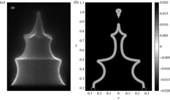
Reference Santosh and Lieuwen2008). A qualitative comparison with experimental results is shown in figure 5.
Flame wrinkling due to vortex formation and roll up. (a) Experimental forced conical flame image, reprinted from Karimi et al. (Reference Karimi, Brear, Jin and Monty2009), with permission from Elsevier. (b) The
 $G$
-field obtained from a numerical simulation of a forced conical flame. In both cases, the forcing is harmonic, with a frequency
 $\mathit{St}=20/(2{\rm\pi})$
and an amplitude
 $A=0.3$
. The flame contour
 $G=0$
is highlighted and it qualitatively reproduces experimental results.

The heat released by the flame is evaluated through
 $$\begin{eqnarray}Q(A,t)\equiv 2{\rm\pi}{\it\rho}s_{L}^{0}h_{R}\iint _{\mathscr{D}}\left(1-\mathscr{L}{\it\kappa}\right)\left|\boldsymbol{{\rm\nabla}}G\right|{\it\delta}(G)r\,\text{d}r\,\text{d}x.\end{eqnarray}$$
Heat release fluctuations
 $q^{\prime }(A,t)=Q(A,t)-\overline{Q}$
are decomposed into Fourier modes
 $$\begin{eqnarray}q^{\prime }(A,t)=\mathop{\sum }_{k=1}^{\infty }q_{k}^{\prime }(A)\cos (2{\rm\pi}\,k\mathit{St}\,t+{\it\varphi}_{k}(A)).\end{eqnarray}$$
Since we are looking for harmonic cycles, we consider only the first harmonic contribution in the Fourier transform of heat release fluctuations:
 $$\begin{eqnarray}\hat{q}^{\prime }(\mathit{St},A)\approx q_{1}^{\prime }(A)\text{e}^{\text{i}{\it\varphi}_{1}(\mathit{St},A)}.\end{eqnarray}$$
The FDF is defined by
 $$\begin{eqnarray}\mathscr{F}(\mathit{St},A)\equiv \frac{\hat{q}^{\prime }(\mathit{St},A)/\overline{Q}}{\hat{u} ^{\prime }(A)/\overline{u}},\end{eqnarray}$$
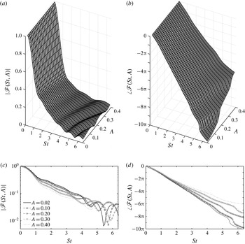
and is shown in figure 6. It contains the features that are characteristic of describing functions of conical flames: unitary gain and a linear behaviour at small frequencies, the presence of amplitude-dependent zeros due to destructive wave interference, and a general monotonic decrease of the phase, typical of time-delayed systems. They are described in detail in experimental and numerical studies (Schuller et al. Reference Schuller, Durox and Candel2003; Karimi et al. Reference Karimi, Brear, Jin and Monty2009).
FDF gain (a,c) and phase (b,d) of the heat release rate of a laminar, conical flame to velocity fluctuations. The flame aspect ratio is
 ${\it\beta}=6$
and curvature effects on the flame speed are accounted for, with a non-dimensional Markstein length
 $\mathscr{M}=0.02$
. Here (a,b) and (c,d) show the same data.

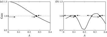
We can now study the stability of the thermoacoustic system. The FDF is closed in a positive feedback loop with the acoustics. Figure 7 shows the amplitude dependence of the gain of the closed loop functions
 $H_{x_{f}}(\mathit{St},A)\equiv \mathscr{F}(\mathit{St},A)G_{x_{f}}(\mathit{St})$
at two frequencies. It gives insight into the possible types of bifurcations of the thermoacoustic system. In particular, we can predict that supercritical bifurcations are expected at low oscillation frequencies, whereas a subcritical response can be found at higher frequencies.
Schematic stability analysis based on the closed-loop gain
 $|H_{0.51}(\mathit{St},A)|$
amplitude dependence for two
 $\mathit{St}$
values: (a) 1.91; (b) 4.97. (a) At small frequencies, a monotonical decay of the gain suggests that the system can be either linearly stable (if the gain at
 $A=0$
is less than one) or supercritically unstable and saturate to a limit cycle. (b) At higher frequencies, the gain does not monotonically decay and subcritical instabilities may exist, as well as multistability. Filled and empty circles indicate stable and unstable limit cycles (fixed points at zero amplitude), respectively.

However, the condition described in figure 7 is only a necessary condition for the existence of limit cycles. In order to correctly predict limit cycles amplitudes and frequencies, we have to consider the closed-loop plant phase dependence as well. On saturated limit cycles the growth rate
 ${\it\sigma}$
of thermoacoustic modes is zero, and harmonic oscillations are found for the pairs
 $(A,\mathit{St})$
that satisfy the dispersion relation (harmonic balance):
 $$\begin{eqnarray}H_{x_{f}}(\mathit{St},A)\equiv \mathscr{F}(\mathit{St},A)G_{x_{f}}(\mathit{St})=1.\end{eqnarray}$$
We determine the stability of limit cycles by looking at the change in sign of the growth rate around the saturated amplitudes (Schmid et al.
Reference Schmid, Blumenthal, Schulze, Polifke and Sattelmayer2013). Growth rate and frequency maps away from limit cycles are determined by fitting the FDF to a state-space model for each amplitude section, and replacing
 $\mathit{St}$
with the Laplace variable
 $s$
in the dispersion relation (4.6).
We investigate the stability of modes with a maximum frequency
 $\mathit{St}_{max}=40/(2{\rm\pi})\approx 6.37$
, which is the maximum frequency at which we forced the system when evaluating the FDF. Note that, according to the harmonic balance condition (4.6), an oscillation can arise only if the product between the FDF and the acoustic transfer function’s gain exceeds unity. The gain of the laminar, conical FDF shown in figure 6 does not exceed unity, so oscillation frequencies for this flame are always expected to be close to an acoustic eigenfrequency; this is verified in § 6 (see figure 12). Therefore, we label thermoacoustic modes by the acoustic mode with the closest frequency.
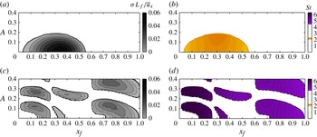
Two thermoacoustic modes can have a positive growth rate in the range of parameters considered. The first mode (figure 8
a,b) has a positive growth rate in the region
 $0.04\leqslant x_{f}\leqslant 0.56$
. Within this region, fixed point solutions are unstable and small perturbations cause oscillations with a frequency
 $\mathit{St}\in (2.1,2.3)$
to grow in amplitude, until they saturate on stable limit cycles indicated with solid lines. Two supercritical Hopf bifurcations are located at the edges of this region. The second mode (figure 8
c,d) exhibits several supercritical and subcritical Hopf bifurcations, fold points and multistable regions. Stable and unstable limit cycles are identified, and oscillate at a frequency in the range
 $\mathit{St}\in (4.5,6.3)$
. In some cases, the saturation amplitude of the oscillations exceeds the maximum forcing amplitude we have considered when obtaining the FDF, and cannot be predicted from our data.
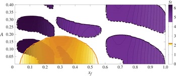
Harmonic balance stability analysis of the first (a,b) and second (c,d) thermoacoustic modes. (a,c) Positive growth rates of the modes as a function of the velocity fluctuations amplitudes. Moving from low to high amplitudes, if the growth rate passes from positive (negative) to negative (positive), a stable (unstable) limit cycle is found. (b,d) Frequency maps of regions with positive growth rates.

Figure 9 superposes the frequency maps of the positive growth rate regions of the two modes. In some regions, both thermoacoustic modes have positive growth rates. This raises questions about the physical interpretation of results obtained with the harmonic balance analysis. The main assumption, that the limit cycles are harmonic, becomes particularly weak if more than one mode is linearly unstable. If both modes grow, how does the flame behave? If both modes have incommensurate frequencies, is the final attractor of the thermoacoustic system a limit cycle? If the oscillations are non-harmonic, how different is their amplitude compared with those predicted with the FDF? These questions cannot be tackled in a single-mode frequency domain framework, and different approaches need to be used.
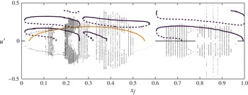
Harmonic balance bifurcation diagram. The amplitudes and frequencies of the thermoacoustic modes with non-negative growth rate are shown while varying the position of the flame in the duct. Supercritical and subcritical bifurcations of two thermoacoustic modes are observed. Stable and unstable limit cycles are indicated with solid and dashed lines, respectively. In some regions, both modes have a positive growth rates.

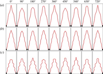
Instantaneous self-excited flame images at different flame locations over two cycles of the power spectral density (PSD) dominant frequency. (a) At
 $x_{f}=0.51$
the system exhibits periodic, non-harmonic oscillations, with a dominant frequency associated with the first thermoacoustic mode. (b) At
 $x_{f}=0.95$
the oscillations are still periodic, but they are associated with the second thermoacoustic mode, with a higher frequency; the characteristic flame perturbation wavelength varies accordingly. (c) At
 $x_{f}=0.43$
the system has undergone a Neimark–Sacker bifurcation: two incommensurable frequencies describe the motion, which is aperiodic and the flame shape is never exactly the same.

5. Nonlinear dynamics in the time domain
The general behaviour of thermoacoustic oscillations is not limited to harmonic limit cycles. Several experimental and numerical studies report that small variations in a single parameter in the thermoacoustic state, such as the equivalence ratio, position of the flame in a duct, intensity of the mean flow, lead to profound changes in the oscillations dynamics, which can exhibit for example quasiperiodic and chaotic behaviour (Gotoda et al. Reference Gotoda, Nikimoto, Miyano and Tachibana2011; Kabiraj & Sujith Reference Kabiraj and Sujith2012; Kashinath et al. Reference Kashinath, Waugh and Juniper2014). In this section we use two different time domain techniques to analyse the thermoacoustic system that was investigated with the harmonic balance technique in the previous section. We interpret the results with nonlinear time series analysis and Floquet theory.
5.1. Time-marching
Analysis in the time domain does not require the restrictive assumptions required for analysis in the frequency domain, particularly that the acoustic oscillations are harmonic. We couple the acoustic state-space models with the
 $G$
-equation dynamics (2.6) and we time integrate the thermoacoustic system. The acoustics induce axial velocity perturbations at the base of the flame. Continuity and advection equations are integrated numerically in the flame domain. The
 $G$
-field is updated. The unsteady heat release is evaluated through (4.2). This acts as a source in the acoustic equations, closing the loop. The analysis is performed by integrating the thermoacoustic dynamics from fixed points for 350 non-dimensional time units in the range
 $0\leqslant x_{f}\leqslant 1$
, with steps of
 ${\rm\Delta}x_{f}=0.01$
, and a higher resolution in regions of interest. For
 $0.65\leqslant x_{f}\leqslant 0.78$
we have also integrated the thermoacoustic response starting from a highly perturbed initial condition, in order to analyse the subcritical response of the system. The time series of acoustic velocity fluctuations at the flame position are stored and used for post-processing analysis. The resulting bifurcation diagram (figure 13) is shown in § 6.
Figure 10 shows instantaneous flame shapes at different flame locations over two cycles of the dominant oscillation frequency. We observe that for some flame locations,
 $x_{f}=0.51,0.95$
, the flame shape evolution repeats itself after one cycle, i.e. the system exhibits non-harmonic limit cycle oscillations. On the other hand, at
 $x_{f}=0.43$
the flame shape does not repeat itself, meaning that the motion is aperiodic; at least two incommensurable frequencies are governing the dynamics, which cannot be described by a limit cycle.
5.1.1. Nonlinear time series analysis
To further characterize the system, we use methods from nonlinear time series analysis (Gotoda et al.
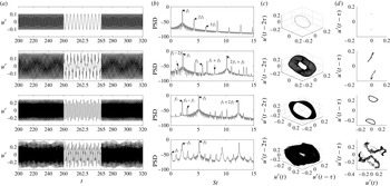
Reference Gotoda, Nikimoto, Miyano and Tachibana2011; Kabiraj & Sujith Reference Kabiraj and Sujith2012). Figure 11 left panels show the time series of velocity fluctuations at the flame position for different flame locations. Moving from top to bottom, they identify limit cycle, frequency-locked, quasiperiodic and chaotic oscillations, respectively; the region
 $260<t<265$
has been enlarged to highlight the shape of the oscillations. In limit cycles the time trace exactly repeats itself after a period
 $T$
. Frequency-locked oscillations exhibits several peaks and troughs, and the time series exactly repeats itself after a certain number of oscillations, which are characterized by two well-defined time scales. Also in the quasiperiodic time trace we can identify two time scales, but on close inspection these oscillations never repeat themselves. Finally, in chaotic solutions it becomes harder to distinguish precise time scales and the time series is certainly aperiodic.
Characterization of the dynamical behaviour observed in our thermoacoustic model. From top to bottom: limit cycle, frequency-locked, quasiperiodic and chaotic oscillations; (a) saturated time series, (b) PSD, (c) phase space portraits and (d) Poincaré sections. Time series have been expanded between
 $260\leqslant t\leqslant 265$
.

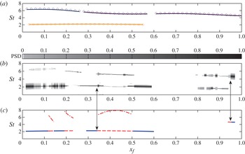
Comparison between predicted frequencies. (a) Circles indicate the first two natural acoustic frequencies of the geometry considered. Lines refer to Strouhal numbers of stable limit cycles found with the harmonic balance technique. (b) Intensity of the normalised PSDs of converged time series. (c) Dominant frequency of cycles obtained with numerical continuation (lines). Dot-dashed lines correspond to the frequency of the incipient unstable mode predicted by Floquet analysis when a Neimark–Sacker bifurcation occurs, as indicated by the arrows.

Time integration bifurcation diagram (dots) and FDF predicted stable and unstable limit cycles (lines). Time series peaks and troughs of the final stable thermoacoustic state are shown as a function of the flame position in the duct. Solid lines at
 $u^{\prime }=0$
indicate linearly stable fixed points.

It is difficult to distinguish between the various types of oscillations just by looking at the temporal evolution of the velocity fluctuations. We use power spectral density (PSD), phase portraits and Poincaré sections to characterize the dynamical behaviour of each thermoacoustic oscillation (Guckenheimer & Holmes Reference Guckenheimer and Holmes1983; Thompson & Stewart Reference Thompson and Stewart2001; Kantz & Schreiber Reference Kantz and Schreiber2004). Figure 11 shows the results of nonlinear time series analysis for each type of dynamics we observe. All of these methods play a role in a detailed discussion of the bifurcations and the nonlinear thermoacoustic regime, which is postponed until §§ 6 and 7.
5.2. Continuation of limit cycles
Time-marching is the most accurate technique to study a nonlinear system. The main shortcoming of time-marching is its computational cost. The transient between an unstable thermoacoustic state and the final stable attractor can pass through several intermediate states and can take a long time (Kashinath et al.
Reference Kashinath, Waugh and Juniper2014). Therefore, there is the need to develop a tool that gives more information than the FDF technique, but that has lower computational cost than time integration. Numerical continuation of limit cycles achieves this. Assuming that a periodic (but not necessarily harmonic) solution is known for a set of thermoacoustic parameters, we can vary one parameter slightly and iteratively solve a linear problem to find a thermoacoustic cycle with the new set of parameters. The use of this technique on low-order models is particularly efficient because the number of relevant degrees of freedom of a thermoacoustic state
 ${\bf\sigma}$
is fairly small,
 $O(10^{3})$
. Matrix-free methods can be used to decrease even further the memory and time required to solve the set of linear equations. Matrix-free methods for limit cycles have been introduced to thermoacoustics by Waugh, Illingworth & Juniper (Reference Waugh, Illingworth and Juniper2013) and have been successfully used in analysing a ducted premixed flame with Fourier–Galerkin acoustics (Waugh et al.
Reference Waugh, Kashinath and Juniper2014).
Let us indicate with
 $[{\bf\sigma}^{0}(0,x_{f}),T^{0}]$
an initial guess for a starting state and period of a thermoacoustic cycle. We integrate the system forward in time over a cycle and compute the residual
 $\boldsymbol{r}^{0}\equiv {\bf\sigma}^{0}(0,x_{f})-{\bf\sigma}^{0}(T^{0},x_{f})$
. Then we iteratively solve the linear problem
 $\unicode[STIX]{x1D645}^{0}{\rm\Delta}{\bf\sigma}^{0}=-\boldsymbol{r}^{0}$
with the Jacobian matrix
 $\unicode[STIX]{x1D645}^{0}$
defined by a shooting iteration:
 $$\begin{eqnarray}\unicode[STIX]{x1D611}_{ij}^{0}\equiv \frac{\partial \left({\it\sigma}_{i}^{0}(0,x_{f})-{\it\sigma}_{i}^{0}(T^{0},x_{f})\right)}{\partial {\it\sigma}_{j}^{0}(0,x_{f})},\end{eqnarray}$$
to find a correction
 $[{\rm\Delta}{\bf\sigma}^{0},{\rm\Delta}T^{0}]$
to be added to the initial guess and obtain a new starting state
 $$\begin{eqnarray}\left[{\bf\sigma}^{1}(0,x_{f}),T^{1}\right]=\left[{\bf\sigma}^{0}(0,x_{f}),T^{0}\right]+\left[{\rm\Delta}{\bf\sigma}^{0}(0,x_{f}),{\rm\Delta}T^{0}\right]\end{eqnarray}$$
which is closer to a limit cycle solution. The process is iterated until the residual falls below a threshold value, set to
 $5\times 10^{-4}$
.
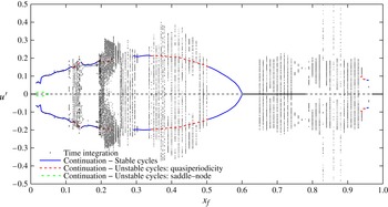
Thermoacoustic bifurcation diagrams obtained with time integration (dots, see figure 13) and numerical continuation (lines). The bifurcation parameter
 $x_{f}$
is the dimensionless flame’s position in the combustion chamber. The amplitude of self-excited acoustic velocity fluctuations is shown. Lines connect the absolute maximum and minimum amplitudes of cycles found with numerical continuation: solid lines indicate stable limit cycles, dashed lines two different types of limit cycle instability mechanisms, saddle–node (dot-dashed) and Neimark–Sacker (dashed).

Matrix-free methods are used to solve the linear problems
 $\unicode[STIX]{x1D645}^{n}{\rm\Delta}{\bf\sigma}^{n}=-\boldsymbol{r}^{n}$
(
 $n$
indicates the
 $n+1$
shooting iteration) by means of an implementation of the generalized minimal residual (GMRES) algorithm (Saad & Schultz Reference Saad and Schultz1986). Solution approximations
 ${\rm\Delta}{\bf\sigma}^{n}\approx {\rm\Delta}{\bf\sigma}_{k}^{n}$
are evaluated on a
 $k$
-dimensional Krylov subspace by minimising the GMRES residual
 $$\begin{eqnarray}{\it\beta}_{k}^{n}\equiv \Vert -\boldsymbol{r}^{n}-\unicode[STIX]{x1D645}^{n}{\rm\Delta}{\bf\sigma}_{k}^{n}\Vert .\end{eqnarray}$$
The algorithm is stopped when the residual (5.3) falls below a predefined threshold,
 ${\it\beta}_{k}^{n}\leqslant 5\times 10^{-2}$
. One period of time-marching integration is required whenever we add a new dimension to the Krylov subspace. For our system, convergence is achieved within
 $k=30$
iterations. Considering that the thermoacoustic state is formed from around 600 variables, the matrix-free method is 20 times faster than the computation of the entire Jacobian.
Once two (or more) limit cycles have been found for different values of the bifurcation parameter, we can improve the initial guess of the next cycle by extrapolating the variable values in the thermoacoustic state, allowing a further speed-up in the calculations. The bifurcation diagram obtained with numerical continuation is shown in figure 14. In some regions no solution is shown because limit cycles do not exist, or because the continuation algorithm does not converge. This happens when the flame shape becomes very complicated, i.e. when the flame is oscillating at high frequencies, and is a technical problem with our implementation, not the technique in general. Nevertheless, we have been able to track limit cycles in most of the parameter regions we have considered.
5.2.1. Floquet analysis of limit cycles
We can straightforwardly analyse the stability of cycles found with continuation by means of Floquet theory (Guckenheimer & Holmes Reference Guckenheimer and Holmes1983). Floquet multipliers are complex numbers associated with the linear response of limit cycle oscillations to perturbations. If one of them has a magnitude larger than one, the cycle is unstable. Thus, bifurcation locations and types are found by studying when and where Floquet multipliers cross the unit circle. We evaluate numerically the four Floquet multipliers with the largest magnitude. If a multiplier crosses the circle at
 $+1$
, a limit point of cycle (LPC) is found, meaning that the limit cycle branch changes its stability; this corresponds to cyclic fold or saddle–node bifurcations. Period-doubling (flip) bifurcations happen when a Floquet multiplier crosses the circle at
 $-1$
. Finally, Neimark–Sacker (secondary Hopf) bifurcations are found when a pair of complex multipliers crosses the unit circle. The next section contains a discussion on the location of the bifurcations predicted by Floquet theory.
6. Comparison between frequency and time domain results
In this section we compare the results from the three types of analysis. We start by comparing the oscillation frequencies on stable attractors. Then we compare the results obtained with the harmonic balance against those obtained with time-marching. In particular, we examine the location of bifurcation points and the amplitudes of oscillations. Then we compare the results obtained with time-marching against those obtained with continuation.
6.1. Quasi-linear regime: frequency of oscillations
Figure 12(a) shows the frequencies of stable limit cycles found with the harmonic balance method. It shows that the predicted limit cycle frequencies are always very close to the acoustic natural frequencies, as we had anticipated when discussing the FDF. In this analysis, the oscillation frequencies are well-defined because the cycles are harmonic. On the other hand, oscillations in the time domain are not necessarily harmonic. For time-marching simulations, we compute the PSDs of steady-state oscillations and normalise them with respect to the intensity of the highest peak. We assign to the PSDs intensity at each frequency a colour: the higher the intensity, the darker the colour. For each vertical slice of figure 12(b), the black region indicates the frequency at which we have the highest peak, and grey regions are secondary peaks. For numerically continued cycles, which are plotted in figure 12(c), we plot only the fundamental oscillation frequency. Solid lines indicate stable cycles and dashed lines indicate unstable cycles, which have a complex pair of Floquet multipliers with magnitude larger than one, i.e. cycles that have undergone a Neimark–Sacker bifurcation. For these cycles, Floquet theory also predicts the frequency of the mode that is linearly unstable around the cycle. These frequencies are plotted in figure 12(c) with dot-dashed lines. They are close to the frequencies in figure 12(b). They are not exactly the same because the frequency shifts as these unstable cycles evolve towards the stable attractor.
The frequencies predicted by the three methods compare favourably. Referring to the time domain simulations, note that the first mode dominates in the region
 $x_{f}<0.6$
, shown by the fact that its PSD intensity is dominant and the second mode never oscillates alone. This is in agreement with the harmonic balance predictions (see figure 9): the fixed point of the first mode is mainly unstable in this region, whereas the fixed point of the second mode is mainly stable. Finite-amplitude oscillations are therefore needed to trigger limit cycles with high frequencies. For
 $x_{f}>0.6$
, the second mode is dominant. However, a major difference between the methods is observed here: the harmonic balance does not predict oscillations of the first mode in this region, but its frequency appears in the time-marching time series. This is probably due to nonlinear effects, which couple the response of the modes and may induce oscillations that cannot be observed when examining the modes one by one. This suggests that, if the thermoacoustic feedback enhances higher harmonics of the nonlinearity, a frequency domain analysis does not accurately predict the system’s nonlinear behaviour.
6.2. Fully nonlinear regime: limit of the harmonic balance
Figure 13 superposes the bifurcation diagram obtained with the harmonic balance (lines, as in figure 9) and that obtained with the time domain (dots). Dots correspond to peaks and troughs of the acoustic velocity time series. Solid lines at
 $u^{\prime }=0$
indicate linearly stable fixed points.
Let us compare results for the region
 $x_{f}>0.6$
in detail. The harmonic balance predicts a supercritical Hopf bifurcation at
 $x_{f}=0.98$
, which ends in a fold at
 $x_{f}=0.61$
. The subcritical Hopf associated with the fold point is located at
 $x_{f}=0.72$
. A second set of stable limit cycles with higher amplitudes is also found within the same range of parameters, and it has a triggering amplitude
 $u^{\prime }\geqslant 0.2$
.
Time-marching simulations qualitatively reproduce this behaviour: the system has a supercritical Hopf bifurcation at
 $x_{f}=0.96$
and the resulting oscillations persist as the flame moves upstream. Figures 13 and 14 show that there are two stable solutions in the region
 $0.65\leqslant x_{f}\leqslant 0.78$
: a stable fixed point and an oscillating solution. Time-marching finds a subcritical Hopf bifurcation at
 $x_{f}=0.78$
. Thus, time-marching simulations confirm the bistability predicted by the harmonic balance in this region.
However, we observe quantitative differences between the two analyses: one of the main problems is that the positions of Hopf and fold bifurcations obtained with the two methods do not exactly match. One reason for this is that the heat release response to forced harmonic oscillations can be very non-harmonic, and it is a large approximation to consider only the contribution of the first harmonic. This is particularly true for high-amplitude oscillations, because the heat release response is highly nonlinear and can affect the position of fold points. However, it cannot explain a shift of the Hopf bifurcations. The latter is probably due to the fact that the frequency domain analysis relies on interpolation and extrapolation in the Laplace variable and amplitude of the FDF data when solving the dispersion relation (4.6). If the FDF is not well-resolved around the most important frequency regions (the frequencies of the thermoacoustic modes), it causes inaccuracies in the harmonic balance predictions. If the interpolation underestimates the FDF gain, then we underestimate also the overall gain of
 $H_{x_{f}}$
in (4.6), and the Hopf bifurcations are shifted. Increasing the FDF frequency and amplitude resolution improves the agreement between the location of the bifurcations, but cannot address the second major difference between the two analysis, which is one of the main objectives of this paper: steady-state solutions found from time-marching are usually not limit cycles. Looking at the corresponding PSDs while moving the flame from
 $x_{f}=1$
to
 $x_{f}=0$
, we observe the appearance of a new frequency incommensurate with the first one at
 $x_{f}=0.94$
, meaning that the oscillations are quasiperiodic. When this happens, the absolute maximum and minimum velocity often greatly exceed those predicted by the harmonic balance method (see figure 13). For some cases (
 $x_{f}=0.83,0.86,0.88$
), we find that another quasiperiodic stable attractor exists with an even higher maximum amplitude of oscillation,
 $u^{\prime }\approx 0.5$
. It is thus possible that the thermoacoustic system exhibits a triggering mechanism between two quasiperiodic attractors, although this phenomenon is not investigated in this study.
Similar features are found in the region
 $x_{f}\leqslant 0.6$
, where the harmonic balance predicts stable and unstable limit cycles of two modes. As mentioned in § 4, there exist parameter regions where the fixed points of two thermoacoustic modes are simultaneously unstable: because of the nonlinearity in the governing equations, a superposition of the mode responses does not represent the correct evolution of the system. We cannot easily infer a criterion from the frequency domain analysis to determine whether the system will oscillate with one of the two frequencies or if the oscillations will be aperiodic. Thus, we conclude that the FDF as was derived here is not suitable for studying the correct nonlinear dynamics. In theory, it would be possible to obtain more accurate solutions by evaluating a multi-input FDF,
 $\mathscr{F}_{N}(\text{i}{\it\omega}_{1},\dots ,\text{i}{\it\omega}_{N},A_{1},\dots ,A_{N})$
, and solving a set of dispersion relations as described by Moeck & Paschereit (Reference Moeck and Paschereit2012). However, although the general methodology remains similar, increasing the number of input variables makes it impractical to evaluate the FDF; already for a dual-input system the FDF depends on four input parameters,
 $\mathscr{F}_{2}(\text{i}{\it\omega}_{1},\text{i}{\it\omega}_{2},A_{1},A_{2})$
, and the experimental or numerical effort needed to calculate it is beyond practical interest.
6.3. Results from numerical continuation
Cycles found with numerical continuation and the harmonic balance fundamentally differ. In numerical continuation, we impose no further constraints on the cycles dynamics other than those included in the governing equations. Therefore limit cycles’ evaluated with numerical continuation are solutions of the thermoacoustic model, not harmonic approximations. In addition, numerical continuation methods reveal the stability of cycles by means of Floquet theory. This is particularly useful because we can predict the location of Neimark–Sacker bifurcations, which cause transitions from periodic to quasiperiodic dynamics.
Results from numerical continuation and time-marching are compared in figure 14. The locations of Hopf and Neimark–Sacker bifurcations predicted by Floquet theory compare extremely well with those found from time-marching analysis. For stable limit cycles, the oscillation amplitudes of the two methods compare well. This is, of course, not the case for unstable limit cycles. Floquet analysis shows the parameter values at which a quasiperiodic solution exists but cannot predict its amplitude. It can be very different from that of the unstable limit cycle, as shown in figure 14.
Although it would be theoretically possible to perform a Floquet analysis in the frequency domain (Basso, Genesio & Tesi Reference Basso, Genesio and Tesi1997), this requires a multi-input FDF, which is prohibitively expensive to evaluate. The results in this section show that numerical continuation combined with Floquet analysis is a useful tool for the analysis of thermoacoustic models.
7. Nonlinear dynamical behaviour
We conclude by looking in detail at the nonlinear dynamical behaviour we observe, and by discussing analogies and differences between the nonlinear regimes of our system and those found in similar experimental and numerical studies.
Our bifurcation diagram (figure 14) can be compared with the one determined in the experiments performed by Kabiraj & Sujith (Reference Kabiraj and Sujith2012), Kabiraj et al. (Reference Kabiraj, Saurabh, Wahi and Sujith2012a
), on which we have based our geometry. Major differences are found between the two diagrams: as an example Kabiraj & Sujith (Reference Kabiraj and Sujith2012) find that the thermoacoustic system is linearly stable for
 $1\leqslant x_{f}\leqslant 0.343$
(however, in the experiments the response of the system to finite perturbations was not investigated), whereas for the same flame position range we observe a wide region of oscillations.
However, we were not expecting any quantitative agreement between the two results, because we have introduced several approximations in our thermoacoustic system. Our flame model is very simplistic and a more detailed model might be needed to accurately reproduce the correct flame dynamics and heat release response. Also, our lack of knowledge about the acoustic reflection coefficients of the experimental set-up might be important: although we have chosen reasonable models for the geometry considered, the real reflection coefficients may differ. For example, if the damping of high-frequency modes were stronger than the one we considered, the instability of the second mode observed in our analysis at the end of the duct would be suppressed. Including experimentally measured reflection coefficients may improve the agreement with experiments.
Nevertheless, we observe some qualitative common features between the two studies. For example, experimental oscillations after the first Hopf bifurcation have a period of about 5.4 ms, which correspond to a Strouhal number
 $\mathit{St}\equiv L_{f}f/\overline{u}\approx 2.4$
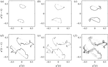
(assuming a flame height of 4 cm). This is consistent with the frequency of the low-frequency mode observed in our numerical analysis (figure 12), which is 2.1. Also, the types of bifurcations found by Kabiraj & Sujith (Reference Kabiraj and Sujith2012) match those we observe: a Hopf bifurcation, followed by a Neimark–Sacker bifurcation, chaos and flame blowout. In the experiments, before chaos an intermittent behaviour associated with the flame lifting off and returning to the burner was observed; we cannot describe this effect because our flame can slide on the burner, but cannot lift off. For the same reason, our low-order simulations cannot model flame blowout, but we reproduce the same route to chaos. By analysing the phase portraits and PSDs of the thermoacoustic time series in the whole range of parameters considered, we identify one type of route to chaos, which is summarised in figure 15. It starts from a quasiperiodic solution, whose Poincaré section (a torus) folds, develops corrugations and finally breaks down. The Poincaré sections of the first and last frames of figure 15 correspond to the time series in the last two rows of figure 11 respectively. By looking at the PSDs, we see that during the torus break-down process a new frequency appears in the spectrum, a sign that a Hopf bifurcation has occurred. Thus, we can identify three subsequent Hopf bifurcations which lead to chaos: at
 $x_{f}=0.59$
a first Hopf bifurcation creates limit cycle oscillations from fixed points; at
 $x_{f}=0.5$
, a secondary Hopf transforms the dynamics into quasiperiodic oscillations; finally at
 $x_{f}=0.42$
a third Hopf bifurcation occurs, and the torus starts to break down, leading to chaotic oscillations. This is the signature of the Ruelle–Takens–Newhouse route to chaos.
Ruelle–Takens–Newhouse route to chaos: (a)
 $x_{f}=0.47$
; (b)
 $x_{f}=0.46$
; (c)
 $x_{f}=0.45$
; (d)
 $x_{f}=0.43$
; (e)
 $x_{f}=0.42$
; (f)
 $x_{f}=0.41$
. Poincaré sections show the creation of a strange attractor from a quasiperiodic solution. The torus of a quasiperiodic solution first folds, then develops corrugations on its surface (c,d) and eventually disintegrates into a strange attractor (e,f).

The same route to chaos, together with the period-doubling route to chaos, is observed by Kashinath et al. (Reference Kashinath, Waugh and Juniper2014). However, they considered as acoustic resonators straight pipes with no area changes, and assumed zero temperature jump across the flame. The same acoustic configuration is considered by Waugh et al. (Reference Waugh, Kashinath and Juniper2014), where fold, period-doubling and Neimark–Sacker bifurcations are identified. As mentioned in § 3.4, in those simple acoustic configurations the natural acoustic eigenfrequencies are all integer multiples of the fundamental duct frequency. This enhances the interaction between the modes: if the fundamental frequency (or a subharmonic) is excited, its harmonics respond as well due to nonlinear effects and, because these harmonics are the resonant frequencies of the higher modes, a coupling between the modes is induced. Thus, one may argue that the highly nonlinear dynamics observed is influenced by the too simplistic geometry. In this study we have shown that this is not the case. Accounting for temperature and area variations, the frequencies of the acoustic modes are no longer equispaced, and the interaction between the modes is reduced. Nevertheless, we still observe very rich nonlinear dynamics.
8. Conclusions
In this study we have developed a low-order thermoacoustic model for premixed flames. Particular care has been taken to describe the acoustics by adapting an existing tool, LOTAN, and casting wave-based frequency response functions into suitable state-space models. This allows us to consider complex acoustic geometries accounting for area and temperature variations, and to easily analyse the stability of a thermoacoustic system both in the frequency and time domains.
An FDF has been evaluated numerically and the stability of this thermoacoustic network has been investigated via the harmonic balance technique. Stable and unstable limit cycles of the first two thermoacoustic modes have been calculated while varying the flame position in the duct. By comparing these results with time-marching simulations, we observe that the harmonic balance technique predicts the onset of instability reasonably accurately and captures the oscillation frequencies well. However, the harmonic balance technique does not predict the amplitudes observed in time-marching results. This is because the combustion model we use, which is based on the kinematic
 $G$
-equation, is highly nonlinear at high amplitudes of oscillations. Consequently, accounting for only the first harmonic component of the heat release fluctuations induces large approximations in the FDF, which is a crucial ingredient in the description of the system in the frequency domain. Second, we observe that neglecting the interaction between the modes can lead to very different results in the dynamical behaviour of the system. If the harmonic balance predicts simultaneous growth of two thermoacoustic modes with incommensurate frequencies, limit cycle oscillations cannot be expected. We observe this in the time domain simulations, in which we observe aperiodic solutions. We determined their dynamical nature by means of nonlinear time series analysis techniques. We identified the position of secondary Hopf bifurcations which lead to quasiperiodic oscillations through Neimark–Sacker bifurcations. We also identified the Ruelle–Takens–Newhouse route to chaos.
Finally, we have applied a numerical continuation algorithm to the system. The method is able to track non-harmonic limit cycles in the parameter space, and does not contain the approximations required when analysing the system in the frequency domain. As a result, the frequencies and amplitudes of cycles obtained with this method approximate results from time-marching simulations very well. Importantly, we can straightforwardly apply Floquet theory on cycles found with numerical continuation and determine their stability. This is particularly important because we can predict the location of Neimark–Sacker bifurcations: when they occur, oscillations cease to be periodic and we need to rely on time-marching methods to have a full characterization of the nonlinear dynamics.
This paper shows that time domain techniques, such as numerical continuation analysis, can be applied to reduced order models containing a
 $G$
-equation flame and complex acoustics. Furthermore, it shows that these techniques are more accurate than the frequency domain techniques that are commonly used in the literature. This is a promising new development for the analysis and understanding of realistic thermoacoustic systems.
Acknowledgements
The authors would like to thank Dr K. Kashinath and Dr I. C. Waugh for comments and support on this paper. This project was funded by the European Research Council through Project ALORS 2590620.