


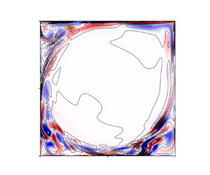




1. Introduction
From a physical standpoint, turbulence is a multi-scale phenomenon exhibiting a wide hierarchy of spatial and temporal scales. This property, coupled with the intrinsic nonlinearity of the governing equations, poses considerable difficulties to its modelling and analysis. One of the major challenges to obtain a satisfactory mathematical description of this phenomenon arises from the fact that the dynamics of flow structures at a particular length or time scale cannot be examined in isolation without also considering at the same time the whole hierarchy of complementary scales (Domaradzki et al. Reference Domaradzki, Liu, Härtel and Kleiser1994). In fact, nonlinear interactions between triads of scales play a fundamental role as they are the main driver of energy transfer between coherent structures (Pope Reference Pope2001; Moffatt Reference Moffatt2014). In turn, the organisation of triadic interactions has a direct influence on the physics of a number of flow phenomena, such as direct and inverse energy cascades (Kolmogorov Reference Kolmogorov1991), or transition to turbulence (Craik Reference Craik1971; Rempfer & Fasel Reference Rempfer and Fasel1994a,Reference Rempfer and Faselb) in different flow configurations (Schmidt Reference Schmidt2020). Overall, this property makes the development of computationally efficient and physically interpretable reduced-order dynamical models a challenging task.
Historically, the study of triadic interactions has been conducted by first employing an appropriate decomposition technique to educe coherent structures from the turbulent motion and then characterising the intensity of the intermodal couplings through the perspective of the resulting Galerkin model (Noack et al. Reference Noack, Schlegel, Ahlborn, Mutschke, Morzyński, Comte and Tadmor2008). For homogeneous isotropic turbulence, Fourier modes provide an optimal representation (Brasseur & Wei Reference Brasseur and Wei1994; Laval, Dubrulle & Nazarenko Reference Laval, Dubrulle and Nazarenko1999), but for flows in complex geometries, modes identified from data with proper orthogonal decomposition (POD) (Rempfer & Fasel Reference Rempfer and Fasel1994a; Couplet, Sagaut & Basdevant Reference Couplet, Sagaut and Basdevant2003) or with frequency domain decomposition methods (Schmid Reference Schmid2010; Towne, Schmidt & Colonius Reference Towne, Schmidt and Colonius2018; Symon, Illingworth & Marusic Reference Symon, Illingworth and Marusic2020) have been often adopted. One of the key findings of such studies is that energy transfers are not uniformly distributed in modal space. In fact, not all interactions have the same importance and energy flows along preferential directions. Specifically, there is evidence suggesting that the nonlinear interaction pattern among coherent structures is often sparse. In other words, the evolution of structures at a certain length scale depends predominantly upon a subset of all other structures (Kraichnan Reference Kraichnan1971; Ohkitani Reference Ohkitani1990; Brasseur & Wei Reference Brasseur and Wei1994), and the influence of interactions with the complementary set of structures can be neglected generally with minor global effects. This behaviour has been observed for a multiplicity of different flows, ranging from bluff body wakes (Jin, Symon & Illingworth Reference Jin, Symon and Illingworth2021) to transitional boundary layers (Rempfer & Fasel Reference Rempfer and Fasel1994a,Reference Rempfer and Faselb) and separated flows (Couplet et al. Reference Couplet, Sagaut and Basdevant2003). However, these studies have focused typically on the interaction between modes educed using a predetermined flow decomposition technique that does not necessarily capture faithfully or optimally the aforementioned physics of scale interactions, since no information regarding nonlinear mechanisms that may produce such interactions is utilised in the decomposition. Hence rationalising scale interactions in these models and identifying relevant physical mechanisms may be challenging, especially in high-dimensional systems Schmidt (Reference Schmidt2020).
In a previous work (Rubini, Lasagna & Da Ronch Reference Rubini, Lasagna and Da Ronch2020b), we utilised  $l_1$-based regression methods (Brunton, Proctor & Kutz Reference Brunton, Proctor and Kutz2016; Loiseau & Brunton Reference Loiseau and Brunton2018) to extract sparsity patterns in the intermodal energy transfers in large Galerkin models of multi-scale flows, to construct sparse, computationally efficient and interpretable models.
This technique consists of calibrating all model coefficients by solving a regression problem (Cordier, El Majd & Favier Reference Cordier, El Majd and Favier2010) augmented with a term that penalises the  $l_1$ norm of the coefficients vector. This type of penalisation is known to promote sparse solutions (Tibshirani Reference Tibshirani1996, Reference Tibshirani2013), and thus results in calibrated models where weak triadic interactions that do not contribute significantly to the overall dynamics are pruned. However, a rigorous connection between the modal structures and the projection model is necessarily lost, since the procedure involves calibrating model coefficients without modifying the basis functions. Hence the analysis of energy paths in the model is not necessarily consistent with the spatial structure of the basis functions. In addition, it was demonstrated that the organisation and sparsity of energy interactions is not invariant with respect to a change of the basis functions utilised for the analysis of the energy budget.
One avenue in this direction that has been explored recently is to utilise sparse coding methods (Olshausen & Field Reference Olshausen and Field1996) and sparse principal component analysis (Jolliffe, Trendafilov & Uddin Reference Jolliffe, Trendafilov and Uddin2003) to encode sparsity directly in the spatio-temporal structure of the reduced basis. For instance, Deshmukh et al. (Reference Deshmukh, McNamara, Liang, Kolter and Gogulapati2016) utilised sparse coding techniques to develop a modified version of POD, producing a compact representation that spans all scales of the observed data. To this end, the authors augmented the POD variational statement with a sparsity-promoting  $l_1$ penalisation term on the temporal coefficients matrix. This forces the temporal coefficients to display a marked intermittent character to capture local dynamics, i.e. periods of activity alternated with periods of low amplitude, with only a subset of the entire set active at any instant. However, the orthogonality between modes is not necessarily preserved. Erichson et al. (Reference Erichson, Zheng, Manohar, Brunton, Kutz and Aravkin2020) generalised the same approach and proposed more efficient computational algorithms for its solution that include orthogonality constraints for the spatial modes. The authors demonstrated that this formulation can be a useful diagnostic tool for problems with rich spatio-temporal behaviour, since it can provide a cleaner data description by identifying localised spatial structures in the data and can disambiguate between distinct time scales. However, spatially or temporally localised modal structures obtained using these techniques may not result directly in a sparser triadic interaction pattern once Galerkin projection is performed. In fact, these techniques utilise only flow data, and it is unclear if this is sufficient to capture the sparse nature of scale interactions.
In this paper, we attempt to bridge this gap. We propose a novel sparsification method in which the goal is to seek directly modal structures that capture energy transfer mechanisms efficiently. More precisely, we seek a new basis set that produces a sparse quadratic coefficient tensor regulating triadic interactions, without the need for an a posteriori tuning based on  $l_1$-based regression. The computational approach is inspired by the subspace rotation technique of Balajewicz, Dowell & Noack (Reference Balajewicz, Dowell and Noack2013) and Balajewicz, Tezaur & Dowell (Reference Balajewicz, Tezaur and Dowell2016), where a small rotation of the POD subspace was sought to absorb the unresolved dissipative scales into the basis functions and stabilise the long-term behaviour without the need for empirical eddy-viscosity terms. Here, the key idea is to seek a small rotation of the original POD subspace to alter and sparsify energy transfer paths. In practice, the rotation is found by solving a constrained optimisation problem, minimising the loss of energy optimality subject to a constraint on the sparsity of the quadratic coefficient tensor. We refer to this method as a priori sparsification, since sparse characteristics are obtained before the projection step, not after.
As a demonstration, we use two-dimensional incompressible lid-driven cavity flow with uniform lid velocity at Reynolds number  $Re = 2 \times 10^4$, where fluid motion is chaotic (Auteri, Parolini & Quartapelle Reference Auteri, Parolini and Quartapelle2002). As opposed to flows at lower Reynolds number just beyond bifurcation to time-dependent flow, energy transfers between modal structures obtained with POD are scattered in modal space and dense Galerkin systems with full model coefficient tensors are obtained. This dynamically complex flow exhibiting a ‘light turbulent’ regime represents a suitable benchmark problem to understand how the proposed optimisation procedure captures the sparsity inherent to the energy cascade of a multi-scale flow. The two-dimensional lid-driven cavity flow is also an established test case for the development and validation of model order reduction techniques (Cazemier, Verstappen & Veldman Reference Cazemier, Verstappen and Veldman1998; Terragni, Valero & Vega Reference Terragni, Valero and Vega2011; Balajewicz et al. Reference Balajewicz, Dowell and Noack2013; Deshmukh et al. Reference Deshmukh, McNamara, Liang, Kolter and Gogulapati2016; Arbabi & Mezić Reference Arbabi and Mezić2017; Fick et al. Reference Fick, Maday, Patera and Taddei2018), and we thus consider it here as an exemplar to demonstrate our approach.
The paper is organised as follows. Section 2 outlines the general methodology to generate reduced-order models by Galerkin projection and how energy interactions between modes defining such models can be analysed. Subsequently, the subspace rotation technique to generate sparse models is described. Results are reported in § 3.
2. Methodology
2.1. Galerkin models and energy analysis
We consider the space of square integrable solenoidal velocity vector fields defined over a spatial domain  $\varOmega$, endowed by the standard inner product
 \begin{equation} (\boldsymbol{u},\boldsymbol{v}) := \int_{\varOmega} \boldsymbol{u}\boldsymbol{\cdot}\boldsymbol{v}\,\mathrm{d}\varOmega, \end{equation}
where  $\boldsymbol {u}, \boldsymbol {v}$ are two elements of such space. The resulting
 $\mathcal {L}^2(\varOmega )$ norm is denoted as
 $\|\boldsymbol {u}\|_2 = \sqrt {(\boldsymbol {u}, \boldsymbol {u})}$. Using the time-averaged velocity field
 $\bar {\boldsymbol {u}}(\boldsymbol {x})$ as a base flow, and denoting by
 $\boldsymbol {u}^\prime (t, \boldsymbol {x}) = \boldsymbol {u}(t, \boldsymbol {x}) - \bar {\boldsymbol {u}}(\boldsymbol {x})$ the velocity fluctuation, the
 $N$-dimensional Galerkin ansatz
 \begin{equation} \boldsymbol{u}(t,\boldsymbol{x}) = \bar{\boldsymbol{u}}(\boldsymbol{x}) + \boldsymbol{u}^\prime(t, \boldsymbol{x}) = \bar{\boldsymbol{u}}(\boldsymbol{x}) + \sum_{i = 1}^{N} a_i(t)\,{\boldsymbol \phi}_i(\boldsymbol{x}) \end{equation}
is introduced to describe the space–time velocity field, where  $a_i(t)$ and
 $\boldsymbol \phi _i(\boldsymbol {x})$,
 $i=1,\ldots, N$, are the temporal and global spatial modes, respectively. We assume throughout that the spatial modes form an orthonormal set and satisfy homogeneous boundary conditions on
 $\varOmega$. Reduced-order models are then derived by projecting the Navier–Stokes equations for incompressible flows onto the subspace defined by the spatial modes (Rowley & Dawson Reference Rowley and Dawson2017) using the inner product defined in (2.1).
Considering configurations where the boundaries are either no-slip walls or periodic and do not change over time, the pressure term arising from the projection vanishes identically for solenoidal modes (Schlegel & Noack Reference Schlegel and Noack2015; Lee & Dowell Reference Lee and Dowell2020). The system of coupled nonlinear ordinary differential equations (ODEs)
 \begin{equation} \dot{a}_i(t) = \mathsf{{C}}_i + \sum_{j=1}^N \mathsf{{L}}_{ij}\,a_{j}(t) + \sum_{j=1}^N \sum_{k=1}^N \mathsf{{Q}}_{ijk}\,a_{j}(t)\,a_{k}(t), \quad i=1,\ldots,N, \end{equation}
is then obtained, defining the temporal evolution of the coefficients  $a_{i}(t)$. Here, the tensors
 $\boldsymbol{\mathsf{C}} \in \mathrm {Re}^{N}$,
 $\boldsymbol{\mathsf{L}} \in \mathrm {Re}^{N\times N}$ and
 $\boldsymbol{\mathsf{Q}} \in \mathrm {Re}^{N\times N\times N}$ are defined by suitable inner products involving the spatial modes. In particular, the coefficients are
 $$\begin{gather} \mathsf{{C}}_{i} = \frac{1}{Re}\,(\boldsymbol{\boldsymbol{\bar{u}}},\nabla^2 \boldsymbol{\boldsymbol{\bar{u}}}) - (\boldsymbol{\boldsymbol{\bar{u}}}, \boldsymbol{\boldsymbol{\bar{u}}} \boldsymbol{\cdot} \boldsymbol{\nabla} \boldsymbol{\boldsymbol{\bar{u}}}), \end{gather}$$
 $$\begin{gather}\mathsf{{L}}_{ij} = \frac{1}{Re}\,(\boldsymbol{ \boldsymbol{\phi}}_i,\nabla^2 \boldsymbol{ \boldsymbol{\phi}}_j) - (\boldsymbol{ \boldsymbol{\phi}}_i, \boldsymbol{\boldsymbol{\phi_j} \boldsymbol{\cdot} \boldsymbol{\nabla} \boldsymbol{\boldsymbol{\bar{u}}}}) - (\boldsymbol{ \boldsymbol{\phi}}_i, \boldsymbol{\boldsymbol{\bar{u}} \boldsymbol{\cdot} \boldsymbol{\nabla} \boldsymbol{\boldsymbol{\phi_j}}}), \end{gather}$$
 $$\begin{gather}\mathsf{{Q}}_{ijk} ={-}(\boldsymbol{ \boldsymbol{\phi}}_i, \boldsymbol{\boldsymbol{\phi}}_j \boldsymbol{\cdot} \boldsymbol{\nabla} \boldsymbol{\boldsymbol{\phi}}_k). \end{gather}$$
The expansion (2.2) provides a suitable foundation to examine interactions between coherent structures in complex geometries. Here, we follow established approaches (Rempfer & Fasel Reference Rempfer and Fasel1994b) and analyse such interactions by introducing the modal energies  $E_i(t) = \frac {1}{2}\,a_i(t)\,a_i(t)$,
 $i=1,\ldots,N$. For an expansion consisting of
 $N$ modes, the domain integral of the kinetic energy of velocity fluctuation expressed by the ansatz (2.2) is then given by
 \begin{equation} E(t) = \sum_{i=1}^{N} E_{i}(t). \end{equation}
The instantaneous rate of change of the modal energies is given by
 \begin{equation} \dot{E}_i(t) = \mathsf{{C}}_i\,a_i(t) + \sum_{j = 1}^{N}\mathsf{{L}}_{ij}\,a_{i}(t)\,a_{j}(t) + \sum_{j = 1}^{N}\sum_{k = 1}^{N} \mathsf{{Q}}_{ijk}\,a_{i}(t)\,a_{j}(t)\,a_{k}(t), \quad i=1,\ldots,N, \end{equation}
obtained by multiplying (2.3) by  $a_i(t)$. The right-hand side of (2.6) is composed of three terms describing energy transfers between the hierarchy of modes (Noack et al. Reference Noack, Schlegel, Ahlborn, Mutschke, Morzyński, Comte and Tadmor2008; Noack, Morzynski & Tadmor Reference Noack, Morzynski and Tadmor2011). The first two describe variations of energy due to production/dissipation arising from interactions with the mean flow and from viscous effects. The third term defines variations of energy arising from inviscid nonlinear interactions between triads of modes. Additional insight can be gained by taking the temporal average of (2.6), i.e. by examining the time-averaged energy budget of system (2.3). Exploiting that the temporal coefficients have zero mean as POD modes have vanishing mean, we obtain
 \begin{equation} \sum_j^N \mathsf{{L}}_{ij}\,\overline{a_i a_j} + \sum_{j=1}^N \sum_{k=1}^N \mathsf{{Q}}_{ijk}\,\overline{a_ia_ja_k} = 0, \quad i = 1, \ldots, N, \end{equation}
where the summation over  $j$ in the linear term accounts for the case where temporal coefficients are not uncorrelated in time. Equation (2.7) shows that, on average, the energy balance is regulated by the production/dissipation described in the linear term and by the nonlinear energy transfer rate described by the quadratic term. As explained in Balajewicz et al. (Reference Balajewicz, Dowell and Noack2013), the residual of (2.7) vanishes only when
 $N \to \infty$ and it is generally expected to be positive for finite-dimensional Galerkin models.
Following Rempfer & Fasel (Reference Rempfer and Fasel1994a), to better visualise the relative importance of the triadic interactions in an average, we introduce the tensor  $\boldsymbol{\mathsf{N}} \in \mathrm {Re}^{N\times N\times N}$ with entries
 \begin{equation} \mathsf{{N}}_{ijk} = \mathsf{{Q}}_{ijk}\,\overline{a_i a_j a_k}, \end{equation}
defining the the average nonlinear transfer rate between triads of modes. The study of the organisation and structure of this tensor and how these are altered by the sparsification algorithm is the main focus of this work.
2.2. Subspace rotation technique
To identify the new set of modal structures, we utilise a subspace rotation technique introduced in the context of stabilisation of Galerkin models by Balajewicz et al. (Reference Balajewicz, Dowell and Noack2013) (see also Amsallem & Farhat Reference Amsallem and Farhat2012). Geometrically, this technique consists of seeking a rotation of an  $N$-dimensional POD subspace within a larger POD subspace of dimension
 $M$. The rotation is defined by a transformation matrix
 $\boldsymbol{\mathsf{X}} \in \mathrm {Re}^{M \times N}$, satisfying
 $\boldsymbol{\mathsf{X}}^{\rm T} \boldsymbol{\mathsf{X}} = \boldsymbol{\mathsf{I}}$ to ensure that the rotated spatial basis functions remain an orthonormal set. The rotated basis functions and the associated temporal coefficients, denoted in what follows with a tilde, are expressed as a linear combination of the original POD spatial and temporal modes as
 $$\begin{gather} \displaystyle \tilde{\boldsymbol \phi}_i(\boldsymbol{x}) = \sum_{j=1}^{M} \mathsf{{X}}_{ji}\, {\boldsymbol \phi}_j(\boldsymbol{x}), \end{gather}$$
 $$\begin{gather}\displaystyle \tilde{a}_i(t) = \sum_{j=1}^{M} \mathsf{{X}}_{ji}\,{a}_j(t). \end{gather}$$
It is worth pointing out that finding a new set of modal structures directly would be a much higher dimensional problem to tackle. The number of unknowns would be proportional to the numbers of modes sought multiplied by the number of degrees of freedom of the problem at hand. Seeking new modal structures as a linear combination of POD modes represents a significant reduction in complexity, controllable by varying the dimension  $M$. Using POD modes as building blocks also has the advantage of producing a basis with good energy reconstruction properties.
The linear and quadratic coefficients of the Galerkin system (2.3) obtained by projection on the rotated subspace are then given by the matrix expressions
 \begin{equation} \tilde{\boldsymbol{\mathsf{C}}} = \boldsymbol{\mathsf{X}}^{\rm T} \boldsymbol{\mathsf{C}} \quad {\rm and}\quad \tilde{\boldsymbol{\mathsf{L}}} = \boldsymbol{\mathsf{X}}^{\rm T} \boldsymbol{\mathsf{L}} \boldsymbol{\mathsf{X}}, \end{equation}
while the quadratic coefficients are cubic polynomial functions of the entries of the rotation matrix
 \begin{equation} \tilde{\mathsf{{Q}}}_{ijk} = \sum_{p, q, r=1}^M\mathsf{{Q}}_{pqr}\, \mathsf{{X}}_{pi}\,\mathsf{{X}}_{qj}\,\mathsf{{X}}_{rk},\quad i,j,k = 1, \ldots, N. \end{equation}
In these expressions, the tensors  $\boldsymbol{\mathsf{C}} \in \mathrm {Re}^{M}$,
 $\boldsymbol{\mathsf{L}} \in \mathrm {Re}^{M\times M}$ and
 $\boldsymbol{\mathsf{Q}} \in \mathrm {Re}^{M\times M \times M}$ are the Galerkin coefficient tensors obtained from the
 $M$-dimensional set of original POD modes.
Our goal is to seek a rotation matrix for which the rotated quadratic interaction coefficient tensor  $\tilde {\boldsymbol{\mathsf{Q}}}$ has a sparse structure, i.e. where as many as possible of the quadratic interaction coefficients are identically zero.
At this stage, it is worth noting that any rotation is necessarily accompanied by a loss of average fluctuation kinetic energy reconstructed by the new basis. The energy reconstructed by a set of  $P$ POD modes can be quantified by utilising the average modal energies
 $\lambda _i = \overline {a_i a_i}$,
 $i = 1, \ldots, P$. Arranging them into a diagonal matrix
 ${\boldsymbol \varLambda }_P \in \mathrm {Re}^{P\times P}$, the trace
 ${\rm Tr}( \boldsymbol {\varLambda }_P )$ defines an upper bound for the reconstructed energy for any
 $P$-dimensional set of basis functions, due to well-known optimality properties of POD. Similarly, the energy reconstructed by the rotated basis can be expressed with the average modal energies
 $\tilde {\lambda }_i = \overline {\tilde {a}_i \tilde {a}_i}$,
 $i=1, \ldots, N$, of the rotated temporal coefficients (2.9b) and arranging them into the diagonal matrix
 $\tilde {\boldsymbol {\varLambda }}_N = \boldsymbol{\mathsf{X}}^{\rm T} \boldsymbol {\varLambda }_M \boldsymbol{\mathsf{X}} \in \mathrm {Re}^{N\times N}$. The loss of reconstructed average fluctuation kinetic energy with respect to an
 $N$-dimensional POD subspace is then quantified as
 \begin{equation} \mathcal{J}(\boldsymbol{\mathsf{X}}) = {\rm Tr}( \boldsymbol{\varLambda}_N - \boldsymbol{\mathsf{X}}^{\rm T} \boldsymbol{\varLambda}_M \boldsymbol{\mathsf{X}}). \end{equation}
As observed in Balajewicz et al. (Reference Balajewicz, Dowell and Noack2013), this quantity is necessarily non-negative due to the optimality of the original POD basis, i.e.
 \begin{equation} \overline{\int_\varOmega \|\boldsymbol{u}^\prime(t, \boldsymbol{x})\|^2 \,\mathrm{d}\varOmega} = {\rm Tr}(\boldsymbol{\varLambda}_\infty) > {\rm Tr}(\boldsymbol{\varLambda}_N) \ge {\rm Tr}(\tilde{\boldsymbol{\varLambda}}_N), \end{equation}
where the last equality holds for  $M>N$ in trivial cases only. In addition, the quantity (2.12) is also always identically zero when
 $M=N$, for any
 $\boldsymbol{\mathsf{X}}$, since any linear combination of
 $N$ POD modes necessarily spans the same original
 $N$-dimensional subspace.
To measure sparsity of the quadratic interaction coefficient tensor, we use the  $l_1$ norm operator, denoted as
 $\|{\cdot }\|_1$, in light of the practical intractability of the zero norm in optimisation (Jovanović, Schmid & Nichols Reference Jovanović, Schmid and Nichols2014). Then the trade-off between energy optimality and sparsity is expressed by formulating the following constrained optimisation problem:
 \begin{align} {}\min_{\boldsymbol{\mathsf{X}}} &\quad {\rm Tr}(\boldsymbol{\varLambda}_N - \boldsymbol{\mathsf{X}}^{\rm T} \boldsymbol{\varLambda}_M \boldsymbol{\mathsf{X}}), \end{align}
 \begin{align} {\rm subject to} & \quad \|\tilde{\boldsymbol{\mathsf{Q}}}\|_1 \leq \|\boldsymbol{\mathsf{Q}}\|_1 / \xi, \end{align}
 \begin{align} &\quad \boldsymbol{\mathsf{X}}^{\rm T} \boldsymbol{\mathsf{X}} = \boldsymbol{\mathsf{I}}_{N\times N} , \end{align}
referred to as problem  ${\rm P1}$ in what follows. The role of the objective function (2.14a) is to favour transformation matrices that minimise the loss of energy optimality, producing a set of basis functions with good energy representation ability, as in Balajewicz et al. (Reference Balajewicz, Tezaur and Dowell2016). On the other hand, the constraint (2.14b) encourages sparse solutions, because some entries of
 $\tilde {\boldsymbol{\mathsf{Q}}}$ are shrunk to zero during the solution of (2.14) by the non-differentiability of the
 $l_1$ norm (Friedman, Hastie & Tibshirani Reference Friedman, Hastie and Tibshirani2008; Tibshirani Reference Tibshirani2013). Sparsification of the linear coefficients tensor
 $\tilde {\boldsymbol{\mathsf{L}}}$ should not be expected. Then the weight
 $\xi$ is an arbitrary penalisation parameter that controls the relative
 $l_1$ norm of the rotated quadratic coefficient tensor and the sparsity of the resulting Galerkin model. This parameter ranges from
 $1$ to arbitrarily large values. When it is equal to
 $1$, the
 $l_1$ norm of the rotated tensor is not affected and no sparsification is obtained. Conversely, using larger
 $\xi$ constrains the norm of the rotated tensor to decrease. This promotes sparsity due to the non-differentiability of the
 $l_1$ norm, with a mechanism (see Appendix A) similar to well-known LASSO methods (Tibshirani Reference Tibshirani1996). In addition, different definitions of the sparsification constraint (2.14b) can be used to highlight different physical aspects of the resulting bases. As an example, in an exploratory study we observed that applying the
 $l_1$ norm constraint on
 $\tilde {\boldsymbol{\mathsf{N}}}$ instead of
 $\tilde {\boldsymbol{\mathsf{Q}}}$, it is possible to promote sparsity in the average triadic interaction tensor. Interestingly, with this formulation, sparsification is promoted by penalising the entries
 $\overline {\tilde {a}_i\tilde {a}_j\tilde {a}_k}$ more than the entries of
 $\tilde {\boldsymbol{\mathsf{Q}}}$. As a result, the temporal coefficients display intermittency behaviour similar to what is observed by Deshmukh et al. (Reference Deshmukh, McNamara, Liang, Kolter and Gogulapati2016).
It is worth noting that using the a posteriori LASSO-based sparsification method (Brunton et al. Reference Brunton, Proctor and Kutz2016; Rubini et al. Reference Rubini, Lasagna and Da Ronch2020b), all quadratic coefficients could, in principle, be set to zero by using a large regularisation weight in the LASSO optimisation problem. This is because the constant, linear and quadratic coefficients of the Galerkin model are directly the optimisation variables. In the present case, the model coefficients cannot be modified directly, but the model tuning is performed indirectly through the rotation matrix  $\boldsymbol{\mathsf{X}}$, which is the actual optimisation variable of the problem. The important consequence is that it might not always be possible to find a rotation that sets an arbitrarily large number of model coefficients to zero. This indicates that problem (2.14) might not have a feasible solution if the penalisation weight is too large.
An important characteristic of optimisation problem (2.14) is that while the objective (2.14a) is convex, the sparsity-promoting constraint (2.14b) is not, as it involves cubic polynomials in the optimisation variables, the entries of the transformation matrix  $\boldsymbol{\mathsf{X}}$. Consequently, the solution might not be unique, and several local minima, corresponding to different sets of basis functions, may be obtained by starting the optimisation from different initial guesses. However, as demonstrated in Appendix B, starting the optimisation from small random perturbations of the original POD basis (justified by the need to retain good energy reconstruction properties) produced consistently the same optimal solutions, which will be presented in § 3.
Assuming that a feasible solution of problem (2.14) can be found, the Galerkin model constructed from projection onto the optimal rotated basis does not necessarily possess better long-term temporal stability characteristics than the original POD model. In fact, it is well known that POD-Galerkin models exhibit long-term instability because of the deficit of energy dissipation attributed to the truncation of small dissipative scales (Noack et al. (Reference Noack, Schlegel, Ahlborn, Mutschke, Morzyński, Comte and Tadmor2008), Schlegel & Noack (Reference Schlegel and Noack2015); see also the recent work of Grimberg, Farhat & Youkilis (Reference Grimberg, Farhat and Youkilis2020) for a point against this argument). In the present case, the transformation  $\boldsymbol{\mathsf{X}}$ obtained from solution of (2.14) does not necessarily result in an improved description of dissipative processes. Classically, this issue is cured by introducing, a posteriori, an eddy-viscosity-type term in the Galerkin model (Galletti et al. Reference Galletti, Bruneau, Zannetti and Iollo2004; Noack, Papas & Monkewitz Reference Noack, Papas and Monkewitz2005; Östh et al. Reference Östh, Noack, Krajnović, Barros and Borée2014). However, an a posteriori correction would not remain in the spirit of the present work. We thus favour the subspace-rotation-based stabilisation approach proposed by Balajewicz et al. (Reference Balajewicz, Dowell and Noack2013, Reference Balajewicz, Tezaur and Dowell2016), which can be introduced naturally in the present formulation. In practice, we augment problem (2.14) with the additional implicit constraint
 \begin{equation} {\rm Tr}(\tilde{\boldsymbol{\mathsf{L}}}) = {\rm Tr}(\boldsymbol{\mathsf{X}}^{\rm T} \boldsymbol{\mathsf{L}} \boldsymbol{\mathsf{X}}) ={-}\eta, \end{equation}
where the auxiliary variable  $\eta \in \mathrm {Re}^+$ is chosen such that
 \begin{equation} \chi(\eta) = \frac{\overline{E(t)}-\overline{E_{DNS}(t)}}{\overline{E_{DNS}(t)}} = 0, \end{equation}
i.e. such that the relative difference of the average fluctuation kinetic energies from direct numerical simulation (DNS) and from numerical simulation of the new model vanishes. The variable  $\eta$ controls dissipation mechanisms in the Galerkin model by altering the spectrum of
 $\tilde {\boldsymbol{\mathsf{L}}}$ and ensures long-term stability. As observed by Balajewicz et al. (Reference Balajewicz, Dowell and Noack2013),
 $\eta$ is not known a priori, but can be found in an inner optimisation loop to ensure that the excess average fluctuation kinetic energy defined by
 $\chi (\eta )$ is zero. With this additional constraint, problem (2.14) becomes
 \begin{align} \min_{\boldsymbol{\mathsf{X}}} &\quad {\rm Tr}(\boldsymbol{\varLambda}_N - \boldsymbol{\mathsf{X}}^{\rm T} \boldsymbol{\varLambda}_M \boldsymbol{\mathsf{X}}), \end{align}
 \begin{align} {\rm subject to} & \quad \|\tilde{\boldsymbol{\mathsf{Q}}}\|_1 \leq \|\boldsymbol{\mathsf{Q}}\|_1 / \xi, \end{align}
 \begin{align} &\quad {\rm Tr}(\boldsymbol{\mathsf{X}}^{\rm T} \boldsymbol{\mathsf{L}} \boldsymbol{\mathsf{X}}) ={-} \eta \quad {\rm with} \chi(\eta) = 0, \end{align}
 \begin{align} &\quad \boldsymbol{\mathsf{X}}^{\rm T} \boldsymbol{\mathsf{X}} = \boldsymbol{\mathsf{I}}_{N\times N}. \end{align}
In this formulation, denoted as P2 henceforth, there is still only one free parameter,  $\xi$. The additional constraint guarantees long-term stability but it can be satisfied (i.e. the problem is feasible) only if
 $M > N$. In fact, any rotation
 $\boldsymbol{\mathsf{X}} \in \mathrm {Re}^{N\times N}$ cannot alter the subspace spanned by the original
 $N$ POD modes and the associated description of dissipation mechanisms captured by the model. In what follows, we consider models with ratio
 $M/N = 2$ and 3.
In practice, a small random perturbation of the original  $N$-dimensional POD basis was used as initial guess for the optimisation, and successive optimisation problems for different penalisations
 $\xi$ were started from the solution of the previous problem. Problem (2.17) was solved with the open-source package for nonlinear and non-convex optimisation NLopt (Johnson Reference Johnson2014). We utilised a solver implementing the method of moving asymptotes (MMA) algorithm (Svanberg Reference Svanberg2014), which requires the gradient of the objective function and of the constraints. The key element to make the procedure viable is to evaluate the sparsity-promoting constraint and its gradient as efficiently as possible. A naive implementation requires
 ${O}(M^3 N^3)$ operations for the evaluation of the sparsity-promoting constraint, and
 ${O}(M^4 N^4)$ for the evaluation of its gradient with respect to the rotation
 $\boldsymbol{\mathsf{X}}$, and costs become intractable quickly. A significantly more efficient algorithm to compute these two quantities – with costs scaling as
 ${O}(M N^3 + M^2 N^2 + M^3 N)$ for the evaluation of the sparsity-promoting constraint and its gradient – can be derived and is key to making the procedure viable (see discussion of the method in Appendix C).
One further technical remark is that the sparsity-promoting constraint is a non-smooth function of the transformation matrix  $\boldsymbol{\mathsf{X}}$, posing difficulties for the utilisation of gradient-based optimisation algorithms. One approach is to implement a subgradient descent method, often used for the solution of the LASSO method (Friedman et al. Reference Friedman, Hastie and Tibshirani2008). However, this algorithm can be implemented only if an analytical solution of the optimisation problem is known, which is not the case here. In this work, we used a manual soft-thresholding approach where entries of the rotated tensor
 $\tilde {\boldsymbol{\mathsf{Q}}}$ smaller that the numerical tolerance specified to the gradient-based optimiser (typically
 $tol = 10^{-5}$) are set to zero at the end of the optimisation.
The Galerkin models obtained from solution of (2.17) are then characterised by examining the density of the rotated triadic interaction tensor, defined as
 \begin{equation} \rho = \frac{\|\tilde{\boldsymbol{\mathsf{Q}}}\|_0}{\|\boldsymbol{\mathsf{Q}}\|_0}, \end{equation}
where the  $l_0$ norm
 $\|{\cdot }\|_0$ counts the non-zero elements of a tensor. The density can also be expressed as the average
 \begin{equation} \rho = \frac{1}{N} \sum_{i=1}^N \rho_i, \end{equation}
with the modal densities  $\rho _i = \|\tilde {\boldsymbol{\mathsf{Q}}}_i\|_0 /\|\boldsymbol{\mathsf{Q}}_i\|_0$,
 $i =1, \ldots, N$, being the relative number of non-zero coefficients in the slices
 $\boldsymbol{\mathsf{Q}}_i$ of the quadratic coefficient tensor associated with each modal index. To express the energy captured by the
 $N$-dimensional rotated basis, we also introduce the global energy reconstruction factor
 \begin{equation} e_N = {\rm Tr}(\tilde{\boldsymbol{\varLambda}}_N) / {\rm Tr}(\boldsymbol{\varLambda}_\infty), \end{equation}
a quantity always strictly lower than 1. The density and the reconstruction factor of the rotated Galerkin models depend on the dimensions  $M$ and
 $N$, and on the penalisation weight
 $\xi$. To characterise the effects of these parameters, we visualise the rotated systems on the
 $\rho$–
 $e_N$ plane, similar to the approach used in Rubini et al. (Reference Rubini, Lasagna and Da Ronch2020b).
3. Demonstration: two-dimensional lid-driven unsteady cavity flow
We now apply this methodology to two-dimensional unsteady flow in a lid-driven square cavity. This is the same test case that we utilised in our previous work (Rubini et al. Reference Rubini, Lasagna and Da Ronch2020b) to demonstrate the properties of  $l_1$-based sparsification of Galerkin models.
3.1. Problem definition and proper orthogonal decomposition
The Reynolds number is defined as  $Re = LU/\nu$, where
 $L$ and
 $U$ are the cavity dimension and the (uniform) lid velocity, respectively, and
 $\nu$ is the kinematic viscosity. All physical variables introduced later are scaled with
 $L$,
 $U$ and combinations thereof. We consider the flow regime establishing at
 $Re = 2 \times 10^4$, where the motion is chaotic (Auteri et al. Reference Auteri, Parolini and Quartapelle2002; Peng, Shiau & Hwang Reference Peng, Shiau and Hwang2003). The domain is defined by the non-dimensional Cartesian coordinates
 $\boldsymbol {x} = (x, y)$, and the velocity vector
 $\boldsymbol {u}(t, \boldsymbol {x})$ is defined by the components
 $u(t, \boldsymbol {x})$ and
 $v(t, \boldsymbol {x})$. For visualisation purposes, we introduce the out-of-plane vorticity component
 $\omega = \partial v/\partial x - \partial u/\partial y$.
Numerical simulations were performed in OpenFOAM with the unsteady incompressible flow solver icofoam. The convective and viscous terms are discretised spatially with a second-order finite-volume technique, and the temporal term with a semi-implicit Crank–Nicolson scheme. A grid independence study was performed, examining average and unsteady flow quantities on increasingly finer meshes. The final mesh is composed of  $300 \times 300$ cells, with refinement at the four cavity boundaries. This mesh is sufficiently fine to resolve the unsteady high-shear regions bounding the main vortex and the high vorticity filaments characteristic of two-dimensional turbulence, as well as the spatial structure of the lowest energy POD modes utilised in this study. Similar grid resolutions have been used by Cazemier et al. (Reference Cazemier, Verstappen and Veldman1998) at similar Reynolds numbers.
Two snapshots of the vorticity field obtained from these simulations are shown in figures 1(a,b). Most of the dynamically interesting features in this regime originate at the bottom-right corner of the cavity. Specifically, the secondary vortex in the recirculation zone is shed erratically, producing wave-like disturbances advected along the shear layer bounding the primary vortex. These structures produce a strong quasi-periodic oscillation of the turbulent kinetic energy, as shown in figure 1(c), where the amplitude of the Fourier transform of the fluctuation kinetic energy signal (2.5) is shown, as a function of the Strouhal number  $St = f L / U$, with
 $f$ the dimensional frequency. Due to the chaotic nature of the flow, the energy spectrum has a strong broadband component with energy uniformly distributed across all the frequencies/spatial structures of the flow. This implies that unlike for periodic flows (Noack et al. Reference Noack, Morzynski and Tadmor2011; Symon et al. Reference Symon, Illingworth and Marusic2020), the mean triadic interaction tensor
 $\boldsymbol{\mathsf{N}}$ is dense, with energy transfers highly scattered in modal space. However, the wave-like motion characterising the shear layer dynamics produces a strong energy peak at a characteristic non-dimensional Strouhal number
 $St = 0.7$ and its harmonics.
(a,b) Instantaneous vorticity fields for two different flow snapshots. (c) Amplitude of the Fourier transform of the fluctuating kinetic energy signal (2.5).

From these simulations, we extract  $N_T = 1000$ snapshots after initial transients have decayed, using a non-dimensional sampling period
 $\Delta t = 0.1$. These settings are sufficient to time-resolve adequately the fastest scales of motion as well as to include many shedding events originating at the bottom right corner. The snapshot POD of this dataset is then performed (Sirovich Reference Sirovich1987). The normalised cumulative reconstructed energy (2.20) is reported in table 1 as a function of the mode number
 $N$.
Normalised cumulative energy reconstruction of the original POD basis functions.

3.2. Analysis of energy interaction of the original POD-Galerkin models
Before examining the properties of the sparsified Galerkin models, we first present some aspects of energy transfers of Galerkin models constructed using the original POD modes, using a reference model size  $N=30$. This dimension is chosen as a compromise between the need to observe a sufficient complexity of modal interactions and the need to limit computational costs associated with the solution of the optimisation problem (see scaling of costs in Appendix C). The POD model for
 $N=30$ resolves approximately
 $97\,\%$ of the average fluctuation kinetic energy, which is sufficient to observe a wide dynamic range in the amplitude of the temporal coefficients and in the strength of energy interactions.
Figure 2(a) shows the organisation of the quadratic coefficients  $\boldsymbol{\mathsf{Q}}$. The slice for mode
 $i=1$ is used as an illustrative example; other modes have similar characteristics. The coefficient tensor is dense as most coefficients are non-zero. No clear structure in the distribution of the coefficients can be observed, except for a slight asymmetry where coefficients for
 $k>j$ are often larger in magnitude, for mode
 $i=1$ but also for most of the other modes. This asymmetry is a consequence of the definition of the quadratic coefficient tensor (2.4c), characterising convective transport mechanisms, and the range of spatial length scales described by the POD modes, as already observed in Rubini et al. (Reference Rubini, Lasagna and Da Ronch2020b). One slice of the average energy transfer rate tensor
 $\boldsymbol{\mathsf{N}}$ is reported in figure 2(b) using the base 10 logarithm of the magnitude. All entries of
 $\boldsymbol{\mathsf{N}}$ are generally non-zero, although the intermodal transfers in the Galerkin model are highly organised and the intensity of interactions varies across several orders of magnitude. This is the combined result of the structure of the quadratic coefficients tensor and the complex spectral structure of the temporal coefficients.
Organisation of (a) the quadratic coefficients  $\boldsymbol{\mathsf{Q}}$, and (b) the average nonlinear transfer rate
 $\boldsymbol{\mathsf{N}}$, for mode
 $i=1$. (c) Collective energy transfer rates associated with the four regions defined in (b), as functions of the modal index
 $i$.

To further characterise energy paths, we split the interactions into four regions, denoted as LL, LH, HL and HH, with L and H denoting low and high index modes, respectively. These four regions represent a coarse-grained grouping of energy transfers between scales resolved by the model, assuming that low-index modes map to the largest scales of motion in the cavity, and high-index modes describe small-scale, low-energy features. This property has been verified for certain problems (Couplet et al. Reference Couplet, Sagaut and Basdevant2003; see also discussion in Grimberg et al. Reference Grimberg, Farhat and Youkilis2020) and is confirmed in the present case by visual inspection of the POD modes. We then compute the sum of the magnitudes of the average transfer rates contained in these four regions for each mode, to characterise in a coarse-grained fashion energy transfers between triads of high-energy modes and smaller, dissipative scales. For instance, for the region LL we compute
 \begin{equation} S_{{LL}} = \sum_{j=1}^{n}\sum_{k=1}^{n} |\mathsf{{N}}_{ijk}|. \end{equation}
The subscript on  $S$ in expression (3.1) denotes one of the four regions. The other regions are defined by analogous expressions, differing in the range spanned by the indices
 $j$ and
 $k$. Here, we arbitrarily select the cut-off at half of the spectrum (
 $n=15$), but other choices are possible and do not change the following results qualitatively. For graphical convenience, we define the notation
 $S_{({\cdot })}$ where the dot represents the quantity (3.1) for the four regions defined in figure 2(b). The result of this analysis is shown in figure 2(c), as a function of the modal index
 $i$. First, energy transfers in the regions LL, HL and LH are generally more intense than those in region HH. This follows from the observation that large-scale/large-scale and large-scale/small-scale interactions are more relevant with respect to the small-scale/small-scale interactions, across the entire hierarchy and in a mean sense. In addition, we observe that the interactions LH are always more intense than the HL interactions. This is a consequence of the asymmetry observed previously in the tensor
 $\boldsymbol{\mathsf{Q}}$, and not of the temporal coefficients, due to definition (2.8), where the indices
 $j$ and
 $k$ commute. This lack of symmetry is in agreement with the picture of energy transfers between scales in homogeneous isotropic two-dimensional turbulence (Ohkitani Reference Ohkitani1990; Laval et al. Reference Laval, Dubrulle and Nazarenko1999), where the large scales interact with the small ones in a non-local fashion.
3.3. Model sparsification
We now consider models with dimension  $N=30$, for ratios
 $M/N = 2$ and
 $3$, and examine in more detail the effect of the sparsity-promoting constraint (2.17b). For each ratio, a family of models with different density and reconstructed average kinetic energy is generated by increasing the penalisation parameter
 $\xi$. Optimal solutions are displayed on the
 $1/\xi$–
 $\|\tilde {\boldsymbol{\mathsf{Q}}}\|_1/\|\boldsymbol{\mathsf{Q}}\|_1$ plane in figure 3(a). The red dashed line separates solutions that satisfy the sparsity-promoting constraint (2.17b) (white area feasibility region) from solutions that do not (red area). Note that the stability constraint is satisfied for all points reported in this figure, as we have noted that the optimiser is still able to satisfy (2.17c) when it first fails to satisfy the sparsity-promoting constraint (2.17b).
(a) Visualisation of the sparsity-promoting constraint (2.17b) on the  $1/\xi$–
 $\|\tilde {\boldsymbol{\mathsf{Q}}}\|_1/\|\boldsymbol{\mathsf{Q}}\|_1$ plane. The red region denotes the infeasibility set. (b–d) Plots of
 $\rho$ versus
 $e_N$ for families of models with dimensions
 $N=30, 20, 40$ and ratios
 $M/N = 2, 3$ (open squares and open circles, respectively). The labels in the legends indicate values of
 $M \times N$.

For small penalisation weights, the optimisation problem has feasible solutions that fall on the boundary of the feasibility region. This suggests that rotations of the original POD basis that minimise the energy loss are found on the boundary, i.e. there is competition between sparsification and energy representation. The key feature of figure 3(a) is that there exists a threshold value  $\xi _t$ above which the optimisation problem terminates unsuccessfully in the infeasible region, i.e. no rotation exists that can reduce the
 $l_1$ norm of the rotated quadratic coefficient tensor below
 $\|\boldsymbol{\mathsf{Q}}\|_1/\xi _t$. This is manifested in figure 3(a) by a sudden turn of the solution traces from the feasible region boundary upwards into the red region. This occurs because, for a given dimension
 $M$, there are only a limited number of coefficients in the tensor
 $\tilde {\boldsymbol{\mathsf{Q}}}$ that can be shrunk to zero by any rotation of the basis functions. The threshold value increases with the ratio
 $M/N$, i.e. the
 $l_1$ norm of the rotated coefficient tensor
 $\tilde {\boldsymbol{\mathsf{Q}}}$ can be decreased further when larger dimensions
 $M$ are used. This is arguably a consequence of the fact that higher ratios
 $M/N$ correspond to more degrees of freedom available to the optimiser to ensure that the sparsity constraint is satisfied. It is worth noting that in LASSO-based sparsification methods (Rubini et al. Reference Rubini, Lasagna and Da Ronch2020b), the optimiser operates directly on the model coefficients and feasible solutions can always be found, with all coefficients shrunk to zero in the limiting case. However, highly sparsified models were observed to have little physical significance and poor temporal behaviour. Here, all feasible systems with varying sparsity/energy reconstruction properties are temporally stable and provide physically consistent predictions. This result is an effort to try to develop a methodology to ensure global stability in data-driven models, extending the work done by Kaptanoglu et al. (Reference Kaptanoglu, Callaham, Hansen, Aravkin and Brunton2021).
In figure 3(c,b,d) the trade-off between sparsity and the energy reconstruction properties of the rotated basis is presented on the  $\rho$–
 $e_N$ plane for models constructed with
 $N=20, 30, 40$, respectively. The horizontal line in each panel corresponds to the fraction of reconstructed energy of the original dense POD-Galerkin model. In these panels, squares are used to denote data for
 $M/N = 2$, while circles denote data for
 $M/N=3$. First, it can be observed that systems for
 $\rho = 1$ (
 $\xi =1$) do not reconstruct the entire average fluctuation kinetic energy captured by the original POD basis. This is due to the stability constraint (2.17c), producing a small rotation of the optimal POD basis so that dissipative mechanisms in the Galerkin models to ensure long-term stability are better resolved. Second, when the penalisation
 $\xi$ is increased, sparser models are obtained, with higher ratios
 $M/N$ enabling further reduction in density. This, however, comes at the cost of decreasing the energy optimality of the rotated basis. More importantly, the larger the model size, the more the model can be sparsified without affecting significantly the ability of the new basis to reconstruct the fluctuation kinetic energy. This suggests that the sparsification technique becomes more effective as the model complexity, and the range of scales resolved by the basis, increases. This appears to be a general trend, since similar behaviour was observed in Rubini et al. (Reference Rubini, Lasagna and Da Ronch2020b) using the LASSO-based a posteriori sparsification.
3.4. Analysis of the rotated modal structures
We now move to the analysis of the rotated spatial and temporal basis functions. We analyse a model with  $N=30$,
 $M/N = 3$ and density
 $\rho =0.87$, obtained for
 $\xi =3$ just before the solution falls into the infeasible region in figure 3(a). Figure 4(a) shows the magnitude of the entries of the rotation matrix
 $\boldsymbol{\mathsf{X}}$, found from the solution of (2.17). Figure 4(b) compares the modal energies of the original POD temporal coefficients with those of the rotated modes. Figure 4(c) shows the cosine of the angle between each pair of original and rotated spatial modes,
 $\cos (\theta _i) = (\boldsymbol {\phi }_i, \tilde {\boldsymbol {\phi }}_i)$, which is clearly also the diagonal of
 $\boldsymbol{\mathsf{X}}$, because of the orthogonality constraint (2.17d). The transformation matrix
 $\boldsymbol{\mathsf{X}}$ has large diagonal entries, but significant off-diagonal terms can be observed for
 $i, j \gtrsim 5$. This indicates that the rotated basis functions bear a strong resemblance to the original POD modes, but that the optimisation has introduced into the new basis small-scale, low-energy features to both stabilise and sparsify the rotated Galerkin model. It is observed that the high-energy temporal and spatial modes are not affected significantly by the rotation and do not differ significantly from the original POD modes. For instance, the first pair of modal energies, corresponding to the dominant fluid oscillation in the cavity, is virtually unchanged. Conversely, high-index, low-energy modes are more significantly rotated away from the corresponding original POD mode, and more significant relative differences of the modal energies are observed. We argue that this behaviour derives from the formulation of problem (2.17), constructed with the aim of generating a basis that minimises the energy loss with respect to the energetically optimal POD. As a result, the optimisation leaves mostly unchanged the most energetic modes that contribute more pronouncedly to the overall energy, and rotates by a larger extent the less energetic modes to gain in sparsity and to achieve stability.
Optimisation results for the case  $M/N=3$,
 $N=30$,
 $\xi =3$ (with density
 $\rho = 0.87$). (a) Magnitude of the entries of the transformation matrix
 $\boldsymbol{\mathsf{X}}$. (b) Distribution of the average modal energies of the original (squares) and rotated (circles) basis functions. (c) Cosine of the angle between the modes of the original and rotated basis.

Figures 5(a,d) show the out-of-plane vorticity component  $\omega$ for the original POD spatial mode, and figures 5(b,e) the rotated mode, for indices
 $i=1$ and
 $19$, respectively. Figures 5(c, f) show the absolute value of the difference between the original and rotated modes. As expected, the spatial structure of the first mode is not changed considerably by the rotation. On the other hand, mode
 $i=19$ is more pronouncedly affected by the rotation, with small-scale vorticity features appearing all along the shear layer. We argue that the introduction of small-scale features is a combined effect of the stability constraint (2.17c), which enhances dissipation in the system (Balajewicz et al. Reference Balajewicz, Tezaur and Dowell2016), and of the sparsity-promoting constraint (2.17b) since spatially fluctuating modes, with stronger gradients, are likely more effective to produce globally zero spatial averages involved in the projection coefficients (2.4c).
Vorticity fields of (a) the first original POD mode, (b) the first rotated mode (denoted as  $\tilde {\omega }$), and (c) the absolute value of their difference. Panels (d–f) show the same quantities for mode
 $i = 19$.

The temporal modes are affected in a similar way. This is illustrated in figures 6(a,b), showing the temporal evolution of modes  $a_1(t)$ and
 $a_{19}(t)$ over twenty time units, and in figures 6(c,d), showing their amplitude spectra, respectively. Since the first column of
 $\boldsymbol{\mathsf{X}}$ is close to zero except for
 $\mathsf{{X}}_{11}$, mode
 $a_1(t)$ and its spectral content are not affected appreciably by the rotation, except for a small general decrease of the amplitude due to decrease in energy content (see figure 4b). Conversely, the spectral content of mode
 $a_{19}(t)$ is remodulated by the rotation by introducing higher energy at high-frequency components, consistent with the introduction of small-scale features into the corresponding spatial mode.
(a) Temporal evolution and (c) amplitude spectrum of  $a_1(t)$. (b) Temporal evolution and (d) amplitude spectrum of
 $a_{19}(t)$. Data are reported for the original POD temporal modes and for the rotated modes of the sparse system obtained from formulation P2.

3.5. Interactions identified in the sparse model
The structure of the spatial and temporal modes is only weakly modified by the optimisation, but this is sufficient to introduce sparsity in the rotated quadratic coefficient tensor  $\tilde {\boldsymbol{\mathsf{Q}}}$ and in the rotated average triadic interaction tensor
 $\tilde {\boldsymbol{\mathsf{N}}}$ when the domain integrals (2.4c) and the temporal averages (2.8) are computed.
To visualise how sparsity in these tensors varies when the penalisation weight  $\xi$ is increased, we introduce the tensor
 $\boldsymbol {\xi }$ with entries
 $\xi _{ijk}$ defined as the value of
 $\xi$ in (2.17) at which the corresponding coefficient
 $\tilde {\boldsymbol{\mathsf{Q}}}_{ijk}$ is first shrunk to zero.
Figure 7 shows two slices of  $\boldsymbol {\xi }$ for
 $i=1$ and
 $i=30$, for a model with
 $N=30$ and
 $M/N = 3$. Results in figures 7(a–c) are obtained with the complete formulation P2, including both the stability and sparsity-promoting constraint, while those in figures 7(d–f) are obtained with formulation P1, which includes only the sparsity-promoting constraint. Figures 7(c, f) show the modal density
 $\rho _i$ as a function of the global density
 $\rho$ for four modes across the hierarchy. By using formulation P2, which includes the stability constraint (2.17c), we observe that small-scale/small-scale interactions disappear first, for moderate penalisations, especially for the high-index modes, but generally across the entire hierarchy of modes. Increasing the penalisation, coefficients corresponding to interactions that are local in modal space are pruned progressively, leaving only coefficients capturing non-local interactions with the low-index modes for large penalisations. The key remark is that the structure of the sparsified quadratic coefficient tensor
 $\tilde {\boldsymbol{\mathsf{Q}}}$, solution of the proposed optimisation approach, follows the same pattern displayed by triadic energy interactions shown in figure 2(b), i.e. coefficients corresponding to energetically weak interactions are pruned first, and only relevant interactions are preserved. Interestingly, figure 7(c) indicates that high-index modes can be sparsified more efficiently. This might be related to the fact that high-index modes are also rotated more aggressively during the optimisation, to ensure that the sparsity-promoting constraint (2.17b) is satisfied and with minor effect of the overall energy reconstruction ability.
(a,b) Entries of the tensor  $\boldsymbol {\xi }$ for
 $i=1,30$, respectively, obtained by solving problem P2. (c) Modal densities
 $\rho _i$ as functions of
 $\rho$. In (d–f), the same quantities are shown from solution of the optimisation problem P1.

Nonetheless, considering now the solution obtained from formulation P1 in figures 7(d–f), it is clear that many quadratic coefficients are indeed shrunk to zero during the optimisation, and similar global densities are obtained. However, the sparsity pattern does not have a clear relation with the original structure of energy interactions. By contrast, coefficients corresponding to important energy interactions have been shrunk to zero since the optimisation problem P1 is driven entirely by the sparsity-promoting constraint. While in both formulations the same penalisation on the  $l_1$ norm of the rotated tensor
 $\tilde {\boldsymbol{\mathsf{Q}}}$ is used, formulation P1 lacks any information regarding the dynamics and temporal evolution of the Galerkin model and the structure of intermodal energy transfers. This results in an unphysical equal contraction of all quadratic coefficients, across all modes and independently of the strength of the energy interactions that they represent. The effect of this behaviour can also be noticed in the
 $\rho _i$–
 $\rho$ curves in figure 7( f), where different individual modes are sparsified by a similar amount. Nevertheless, no significant differences are observed between models obtained from the two formulations on the
 $\rho$–
 $e_N$ plane. From a physical standpoint, this suggests that the proposed approach can produce sparse models with realistic physics only if some notion of the flow dynamics is included in the optimisation procedure. In other words, only targeting the sparsity of the rotated coefficient tensor is not conducive to realistic flow models. In the present case, this is achieved through constraint (2.17c). This, however, ensures only that the model reproduces that same average fluctuation energy observed in DNS. Interestingly, this global metric is sufficient to capture correctly the local nature of intermodal energy transfers.
3.6. Temporal integration and energy analysis of the sparsified system
In this section, we analyse the temporal behaviour of the sparse reduced-order models obtained by solving problems P1 and P2, and consider their rotated triadic interactions tensors  $\tilde {\boldsymbol{\mathsf{N}}}$ and the average energy budget of (2.7). The same minimum-density configuration studied in previous sections, with
 $M/N = 3$,
 $N=30$ and
 $\xi = 3$, is considered. This configuration is used here as a representative example of the sparse models obtained with the proposed approach. In fact, the spatio-temporal statistical behaviour of these models is affected only weakly by the regularisation parameter
 $\xi$, but is mostly dominated by the inclusion of the stability constraint, regardless of the sparsity. Models are integrated forward in time with an implicit time-stepping scheme for
 $T = 500$ time units, from an initial condition obtained from one of the snapshots. Figure 8(a) shows the first one hundred time units of the temporal evolution of the turbulent kinetic energy (2.5) for these two models, compared with the evolution from DNS and from the original POD-Galerkin model. Figures 8(b,c) show the probability density function of the same quantity, computed over a longer time span. As expected, the deficit of dissipation in the original POD-Galerkin model produces fluctuation kinetic energy levels approximately two orders of magnitude larger than the reference value from DNS. This behaviour is well known (see e.g. Östh et al. Reference Östh, Noack, Krajnović, Barros and Borée2014; Noack et al. Reference Noack, Stankiewicz, Morzyński and Schmid2016).
(a) Temporal evolution of the integral fluctuation kinetic energy  $E(t)$. The temporal performances of the two sparse models obtained by solving problem (2.14) are compared against DNS and the dense model obtained with Galerkin projection. Panels (b,c) show the probability distribution of the energy
 $E(t)$, obtained for long-time integration of the Galerkin models.

The sparse Galerkin model obtained without the stability constraint (problem P1) also reproduces this behaviour. Interestingly, the sparse model obtained from this formulation spans a much wider range of flow scales than the POD model ( $N=30$ modes are rotated within a space of
 $M=90$ dimensions), but it still displays dynamical behaviour that is usually attributed to a lack of viscous dissipation. This shows that optimising for sparsity alone is not sufficient to obtain physically realistic models, because energy transfers from energy-producing eddies and dissipative structures are not necessarily captured correctly during the optimisation. Conversely, the sparsified and stabilised model obtained from problem P2 has realistic temporal behaviour and resolves correctly the average energy and its fluctuation observed in DNS. This suggests that including in the optimisation information on how modal structures are supposed to interact with each other to satisfy the overall power budget is key to obtaining sparse Galerkin models with adequate predictive ability. Note that the long-term performance of the models obtained in the present work is generally superior to that of models sparsified a posteriori, using a LASSO-based approach (Rubini et al. Reference Rubini, Lasagna and Da Ronch2020b; Rubini, Lasagna & Da Ronch Reference Rubini, Lasagna and Da Ronch2020a). More specifically, LASSO-based models have been found to be temporally accurate over a time span comparable to that of the data used for the sparsification. Conversely, the present a priori sparsified systems are temporally stable for much longer time horizons. In addition, numerical solutions converge to the asymptotic attractor for much larger perturbations of the initial conditions. We argue that this is likely the consequence of enforcing a stronger consistency between the modal structures and the corresponding Galerkin model.
The structure of the nonlinear energy transfer rate tensor  $\tilde {\boldsymbol{\mathsf{N}}}$ for the rotated Galerkin models is reported in figures 9(a–c) and 9(d–f), showing two slices for
 $i=1,30$, respectively. Figures 9(a,d) refer to the model obtained from Galerkin projection onto the original POD subspace and will be used as reference. Here, the temporal coefficients are the projections onto the DNS snapshots. Data for the model obtained from problem P2 are shown in figures 9(b,e), while data for the model obtained with the P1 formulation are shown in figures 9(c, f). For these models, temporal coefficients are obtained from forward integration of the Galerkin models. It can be observed that the model from formulation P2 displays a pattern of interactions consistent with the DNS data projected onto the original POD modes, in terms of both organisation across modes as well as strength. The organisation of the interactions is similar to that in the dense Galerkin model obtained using the a priori stabilisation method of Balajewicz et al. (Reference Balajewicz, Dowell and Noack2013), although a more aggressive reduction in the strength of the interactions between the high-index modes is observed. This might be a physical effect (small scales tend to be advected primarily by the large ones), but a second possible explanation is that this is the product of the optimisation procedure adopted in this work. To meet the sparsity constraint with minimum impact on the energy reconstruction ability of the rotated basis, the optimiser rotates the high-index modes more aggressively, causing higher sparsity in the dynamical equations of modes associated with small scales. By contrast, energy interactions in the model obtained from the formulation P1 are orders of magnitude more intense, across all triads. This is a manifestation of the lack of dissipation and the consequential over-prediction of energy, across all modes. Interestingly, it can be observed that the HL/LH asymmetry observed in figure 2 is preserved throughout the sparsification. Conversely, this physical feature is lost in the a posteriori approach (Rubini et al. Reference Rubini, Lasagna and Da Ronch2020b) for numerical reasons. It is argued that the a priori approach is preferable for systems where the tensor
 $\boldsymbol{\mathsf{N}}$ has a non-trivial structure, because the link between modal structures and energy interaction tensor is fully preserved.
(a–c) Intensity of the average nonlinear energy transfer rate  $\tilde {\boldsymbol{\mathsf{N}}}$ for mode
 $i=1$ in models obtained from projection and formulations P2 and P1, respectively. Panels (d–f) show the same quantity for mode
 $i=30$.

To conclude this section, we analyse the energy budget of the original and rotated Galerkin models, examining the linear and quadratic energy transfer terms in the average energy budget equation (2.7) on a mode-by-mode basis (Noack et al. Reference Noack, Schlegel, Ahlborn, Mutschke, Morzyński, Comte and Tadmor2008). To characterise the total nonlinear energy transfer, we use the quantity
 \begin{equation} \mathsf{{T}}_i = \sum_{j=1}^N \sum_{k=1}^N \mathsf{{Q}}_{ijk}\,\overline{a_ia_ja_k},\quad i = 1, \ldots, N, \end{equation}
satisfying  $\sum _i \mathsf{{T}}_i = 0$ when the quadratic term conserves energy. In addition, the linear energy transfer term is decomposed into its three constitutive components and we use
 $\mathsf{{L}}^{(m)}$ for the
 $m$th term of the definition (2.4b). These are, in order, the viscous dissipation rate and the production and convection rates mediated by ‘macroscopic’ interactions with the mean flow. The average energy flows associated with these terms are displayed in figure 10 as a function of the modal index. Data for three models are reported: the original POD-Galerkin model (figures 10a,d,g,j,m) with temporal modes obtained from projection on the DNS data, the model obtained from the complete formulation P2 at the minimum density (figures 10b,e,h,k,n), and the model obtained from formulation P1 (figures 10c, f,i,l,o). For these two models, temporal coefficients are obtained from long-time integration. All models are constructed with
 $N=30$ and, where applicable,
 $M/N=3$.
Distributions of time-averaged energy flows as functions of the modal index for models with  $N=30$. Data are reported for the original POD-Galerkin model, (a,d,g,j,m), and for the rotated models from formulations P2 and P1, (b,e,h,k,n) and (c, f,i,l,o), respectively. Panels (a–i) include the energy flows associated to the three components of the linear coefficient tensor (2.4b), corresponding to the viscous dissipation rate and the production and convection energy flow mediated by the mean flow. The sum of the linear energy flows is reported in (j–l). The average nonlinear transfer rates are reported in (m–o).

Figures 10(a–i) show the viscous, production and convection components of the linear energy flow term, while their sum is reported in figures 10(j–l). The nonlinear transfer term is reported in figures 10(m–o). It can be observed that all three models describe viscous dissipation effects in a quantitatively similar manner, and that convection is the only other relevant term of the linear energy flow, while the production term is negligible. This result can be explained by noting that the advection of small-scale features on the shear layer bounding the primary vortical structure operated by the mean recirculatory motion is a significant dynamical feature of the lid-driven cavity flow. However, the model obtained with the P1 formulation, where the rotation of the original POD basis is driven only by the requirement to satisfy the sparsity constraint, results in higher average production rates across the entire spectrum of modes. Overall, the linear energy flow term for the original POD-Galerkin model (figure 10j) exhibits a positive net energy flow for the first four modes, corresponding to the dominant structure and flow oscillation in the cavity, but only moderate dissipation in the remaining modes. This results in an imbalance between extraction of energy from the mean flow and dissipation, leading to the over-prediction of kinetic energy as shown in figure 8(a). The mean nonlinear transfer rate  $\mathsf{{T}}_i$ shown in figure 10(m) displays the correct transfer direction, with energy injected from the large scales (negative transfer rate for low-index modes) to the small scales (positive rate for the remaining modes). The model obtained from the solution of the complete formulation P2 (figure 10k) displays a better balance, since a negative net energy flow rate is observed for
 $i > 4$, due to effect of the stability constraint (2.17b). The distribution and direction of the nonlinear transfers is also well preserved, although lower transfer rates are observed for all modes. This results from the combined effect of the sparsity-promoting constraint, which reduces the magnitude of the quadratic coefficients, and the reduction of the modal energies, due to the loss of optimality from the POD. On the other hand, energy transfers in the model obtained from formulation P1, which does not include any dynamical information on the fluctuation kinetic energy budget (2.7), have a significantly different structure. In fact, both the linear and nonlinear transfer rates show a marked increase, and the organisation of energy flows across the hierarchy of modes has lost the original physical character.
These results show that to obtain a sparse model that is consistent with the flow physics observed in direct simulation, it is of paramount importance to retain in the sparsification algorithm some information regarding the temporal dynamics. This is consistent with what was observed by Loiseau & Brunton (Reference Loiseau and Brunton2018), who showed that an additional constraint on the energy conservation is one way to enhance the temporal accuracy of a fluid model reconstructed from data.
4. Conclusions
Scale interactions in turbulent flows are sparse, and the motion at any given length scale depends most prominently on the dynamics of a subset of all other scales. In addition to the recent work of Schmidt (Reference Schmidt2020), this paper is one attempt at developing a model order-reduction technique that leverages this fact, so that the analysis and interpretation of scale interactions in complex flows is facilitated. Here, we have proposed an a priori sparsification approach, whereby a set of basis functions describing coherent structures that interact minimally with one another is sought for. Scale interaction sparsity is then defined by the sparsity of the quadratic coefficient tensor of the Galerkin model constructed from projection on this basis. As opposed to our previous sparsification approach (Rubini et al. Reference Rubini, Lasagna and Da Ronch2020b), where model coefficients corresponding to weak nonlinear interactions between a predetermined set of basis functions are pruned a posteriori using  $l_1$ regression, the present methodology maintains the exact link between the (sparse) Galerkin model and the modal structures utilised for the projection.
In practice, a set of  $N$ basis functions is expressed as a rotation of
 $N$ proper orthogonal decomposition (POD) modes within a larger POD subspace (of dimension
 $M > N$), with the idea of altering energy paths across the model by rotating the subspace utilised for projection whilst minimising the loss of energy representation ability of the original POD basis. The rotation matrix is then found from the solution of a constrained optimisation problem where (i) the energy loss with respect to the original POD basis is minimised, and (ii) an inequality constraint involving the
 $l_1$ norm of the quadratic coefficient tensor associated to the rotated basis promotes sparsity. This formulation is augmented with a further constraint that enforces long-term temporal stability, following the approach of Balajewicz et al. (Reference Balajewicz, Tezaur and Dowell2016). This optimisation problem depends on a single user-controllable parameter controlling the
 $l_1$ norm of the rotated quadratic coefficient tensor and the trade-off between energy reconstruction and sparsity.
To demonstrate the approach, we considered the incompressible two-dimensional lid-driven cavity flow at Reynolds number  $Re = 2 \times 10^4$, where the motion is chaotic and energy interactions are scattered in modal space. Results show that there is competition between sparsification and energy representation, and that this trade-off depends on the model size
 $N$ and the ratio
 $M/N$. In particular, larger models can be sparsified more aggressively with less impact on the energy reconstruction ability. On the other hand, higher sparsity can be obtained by rotating the same
 $N$ POD basis functions within larger subspaces (a higher ratio
 $M/N$), since the increased flexibility allows shrinking to zero a larger fraction of quadratic interaction coefficients. A deeper analysis of energy paths shows that the distribution of intermodal energy transfers in the rotated model is qualitatively similar to that of the original POD-Galerkin system. More specifically, coefficients of the quadratic interaction tensor corresponding to large-scale/large-scale and large-scale/small-scale interactions are preserved, but those defining weaker small-scale/small-scale interactions are shrunk to zero during the optimisation. This result is in agreement with the established picture of triadic interactions in two-dimensional flows and with previous results of sparsification of reduced-order models (Rubini et al. Reference Rubini, Lasagna and Da Ronch2020b). More interestingly, we observed that a physically consistent organisation of the interactions and a stable long-term behaviour can be obtained only by augmenting the sparsification procedure with the temporal stability constraint. In fact, models obtained without such a constraint inherit well-known temporal stability issues displayed by dense POD-Galerkin models.
Some aspects deserve further discussion. Unlike in  $l_1$-regression-based sparsification methods (Loiseau & Brunton Reference Loiseau and Brunton2018; Rubini et al. Reference Rubini, Lasagna and Da Ronch2020b), where the model coefficients are the optimisation variables, here these coefficients are cubic polynomial functions of the optimisation variables, the entries of the rotation matrix. The first consequence is that the optimisation problem is non-convex, and many local optima, i.e. many different sets of basis functions, exist. It was observed that initial guesses close to the original POD basis, i.e. with good energy representation ability, converge repeatedly to the same optimal solution, which has a consistent physical interpretation. Arguably, initial guesses lying farther from the POD might lead to sparser solutions at the cost of a worse energy reconstruction capability. However, the lack of strong uniqueness guarantees (as for many other modal decomposition techniques) may render the approach questionable. Second, it is not possible to shrink to zero an arbitrary number of model coefficients, as the strong link between the basis functions and the Galerkin model must always be maintained. As a result, the present a priori sparsification technique produces relatively denser Galerkin models than the a posteriori LASSO-based approach considered in Rubini et al. (Reference Rubini, Lasagna and Da Ronch2020b) for the same test case. Rotating the original POD basis into higher-dimensional subspaces, with ratio
 $M/N$ higher than that considered in the present work, to further increase sparsity is possible, although it would necessarily result in increased computational costs for the optimisation.
Funding
The authors gratefully acknowledge support for this work from the Air Force Office of Scientific Research (Grant no. FA9550-17-1-0324, Program Manager Dr D. Smith).
Declaration of interests
The authors report no conflict of interest.
Appendix A. Sparsity-promoting effect of the  $l_1$-based constraint

In this appendix we visualise how the  $l_1$ norm appearing in the constraint (2.17b) favours sparse solutions. For simplicity, we use a small (
 $N = 3$,
 $M = 5$) reduced-order model of the lid-driven cavity flow considered in the previous sections. A more formal discussion based on the proximity operator theory can also be formulated, using the classical LASSO formulation as a starting point (Friedman et al. Reference Friedman, Hastie and Tibshirani2008). In figure 11(a), the ratio
 $\|\tilde {\boldsymbol{\mathsf{Q}}}\|_1/\|\boldsymbol{\mathsf{Q}}\|_1$ is shown as a function of the entries
 $\mathsf{{X}}_{23}$ and
 $\mathsf{{X}}_{12}$ of the rotation matrix. When these two parameters are varied, all the other off-diagonal entries of
 $\boldsymbol{\mathsf{X}}$ are set to zero. Several sharp valleys can be observed, arising from the non-smooth nature of the
 $l_1$ norm. Note that
 $\|\tilde {\boldsymbol{\mathsf{Q}}}\|_1/\|\boldsymbol{\mathsf{Q}}\|_1$ is a non-convex cubic function of the entries of the rotation matrix, and several local minima can be identified. Figure 11(b) shows a cut of figure 11(a) along the
 $\mathsf{{X}}_{12}$ coordinate, where minima are identified by the dashed vertical lines. Each minimum corresponds to a point where one of the entries of
 $\tilde {\mathsf{{Q}}}_{ijk}$ crosses the zero axis, as illustrated in figure 11(c). During the optimisation, the sparsity-promoting constraint pushes the solution towards one of these valleys, due to the strong gradient at the point of non-differentiability, resulting in a sparse coefficient tensor
 $\tilde {\boldsymbol{\mathsf{Q}}}$. However, unlike in the a posteriori LASSO-based sparsification methods (Brunton et al. Reference Brunton, Proctor and Kutz2016; Rubini et al. Reference Rubini, Lasagna and Da Ronch2020b), not all quadratic coefficients can be set to zero simultaneously by an arbitrary rotation, as is clear from figure 11(c). In fact, the tensor
 $\tilde {\boldsymbol{\mathsf{Q}}}$ depends nonlinearly on the rotation
 $\boldsymbol{\mathsf{X}}$, while in LASSO-based methods the tensor coefficients are directly the optimisation variables of the problem.
(a) Map of  $\|\tilde {\boldsymbol{\mathsf{Q}}}\|_1/\|\boldsymbol{\mathsf{Q}}\|_1$ projected on the
 $\mathsf{{X}}_{12}$–
 $\mathsf{{X}}_{23}$ plane. (b) One-dimensional cut of the same quantity along the coordinate
 $\mathsf{{X}}_{12}$. (c) The twenty-seven entries of the rotated
 $\tilde {\boldsymbol{\mathsf{Q}}}$ as a function of
 $\mathsf{{X}}_{12}$. The six entries that vanish identically at one of the sharp points of
 $\|\tilde {\boldsymbol{\mathsf{Q}}}\|_1$ are highlighted in red.

Appendix B. Dependence of the solution from the initial condition
Problem (2.17) is non-convex due to the constraint on the  $l_1$ norm of the rotated quadratic interaction coefficient tensor
 $\tilde {\boldsymbol{\mathsf{Q}}}$.
To understand how this feature affects the results of § 3, we consider in this appendix different sets of initial guesses constructed as increasingly larger perturbations of the identity as
 \begin{equation} \boldsymbol{\mathsf{X}} = \begin{bmatrix}\boldsymbol{\mathsf{I}}_{N\times N} \\ \boldsymbol{\mathsf{0}} \end{bmatrix} + \epsilon \boldsymbol{\mathsf{R}}, \end{equation}
with  $\boldsymbol{\mathsf{R}} \in \mathrm {Re}^{M \times N}$ a randomly generated rotation matrix, satisfying
 $\boldsymbol{\mathsf{R}}^{\rm T} \boldsymbol{\mathsf{R}} = \boldsymbol{\mathsf{I}}_{N\times N}$. We generated ten random rotation matrices for five values of
 $\epsilon$ in the range
 $[10^{-8}, 10]$ and solved problem (2.17) by keeping
 $\xi = 2$ to target an intermediate density in the feasibility region, using
 $N = 30$ and
 $M = 90$.
Results are shown in figure 12. Figure 12(a) quantifies the effects of  $\epsilon$ on the average rotation angle
 $\theta$ between columns of the initial guess and those of the matrix
 $[\boldsymbol{\mathsf{I}}_{N\times N}, \boldsymbol{\mathsf{0}}]^{\rm T}$. Circles and vertical bars identify the average and standard deviation of this quantity across the ten different samples. In figures 12(b,c), the largest modal energy
 $\tilde {\lambda }_1$ of the rotated temporal coefficients and the density
 $\rho$ of the optimal Galerkin model, respectively, are shown as functions of the average
 $\theta$. Results show that for small perturbations of the original POD basis, all initial guesses converge to the same solution, since
 $\tilde {\lambda }_1$ and
 $\rho$ are the same (up to the tolerances set in the optimisation). Conversely, initial guesses corresponding to larger (random) rotation of the original POD basis converge to different solutions, corresponding to modal structures with lower reconstruction ability, but similar model density.
Effect of the initial guess on the optimisation results. (a) Relation between the initial guess perturbation size  $\epsilon$ and the average rotation angle
 $\theta$ away from the original POD basis. Mean and standard deviation of (b) the first modal energy
 $\tilde {\lambda }_1$, and (c) density
 $\rho$, from rotated systems obtained from initial guesses of increasing distance from the original POD basis.

Appendix C. Optimisation of tensor operations and scaling of costs
The sparsity-promoting constraint involves polynomial functions of the optimisation variables. An analytical expression of the gradient of this constraint with respect to the rotation  $\boldsymbol{\mathsf{X}}$ can also be obtained, enabling fast gradient-based optimisation to be utilised. In addition, a careful examination of the tensor operations involved in the computation of the constraint and its gradient shows that a significant reduction of the scaling of costs can be obtained by reorganising some tensorial computations and using intermediate temporary variables (see Pfeifer, Haegeman & Verstraete Reference Pfeifer, Haegeman and Verstraete2014). For instance, a naive calculation of all entries of the rotated tensor (2.11), required in the evaluation of the sparsity-promoting constraint (2.14b), takes
 ${O}(M^3 N^3)$ operations since six different nested for loops (one for each index) are involved in total. However, a careful examination of (2.11) shows that the rotated tensor can also be obtained by first introducing the auxiliary temporary tensors
 $\boldsymbol{\mathsf{A}} \in \mathrm {Re}^{M\times M \times N}$ and
 $\boldsymbol{\mathsf{B}} \in \mathrm {Re}^{M\times N \times N}$, and then computing
 $$\begin{gather} \mathsf{{A}}_{qri} = \sum_{p=1}^M \mathsf{{Q}}_{pqr} \mathsf{{X}}_{pi}, \end{gather}$$
 $$\begin{gather}\mathsf{{B}}_{rij} = \sum_{r=1}^M \mathsf{{A}}_{qri} \mathsf{{X}}_{qj}, \end{gather}$$
 $$\begin{gather}\tilde{\mathsf{{Q}}}_{ijk} = \sum_{q=1}^M \mathsf{{B}}_{rij} \mathsf{{X}}_{rk}, \end{gather}$$
with  $i, j, k = 1, \ldots, N$ and
 $q, r = 1, \ldots, M$. Collectively, these steps take only
 ${O}(M^3 N) + {O}(M^2 N^2) + {O}(M N^3)$ operations, as can be inferred from the summation indices.
On the other hand, the gradient of the sparsity-promoting constraint with respect to the entries  $\mathsf{{X}}_{mn}$ of the rotation matrix
 $\boldsymbol{\mathsf{X}}$ requires the computation of
 \begin{equation} \frac{\partial\| \tilde{\boldsymbol{\mathsf{Q}}}\|_1}{\partial \mathsf{{X}}_{mn}} = \sum_{i, j, k =1}^N\frac{\partial \tilde{\mathsf{{Q}}}_{ijk} }{\partial \mathsf{{X}}_{mn}}\, {\rm sign}(\tilde{\mathsf{{Q}}}_{ijk}), \end{equation}
where the gradient  $\partial \tilde {\mathsf{{Q}}}_{ijk} / \partial \mathsf{{X}}_{mn}$ can be expanded using Kronecker's delta
 $\delta _{ij}$ as
 \begin{equation} \frac{\partial \tilde{\mathsf{{ Q}}}_{ijk}}{\partial \mathsf{{X}}_{mn}} = \sum_{p, q, r = 1}^{M}\mathsf{{Q}}_{pqr}(\mathsf{{X}}_{pi}\mathsf{{X}}_{qj} \delta_{kn} \delta_{rm} + \mathsf{{X}}_{pi}\mathsf{{X}}_{rk} \delta_{jn} \delta_{qm} + \mathsf{{X}}_{rk}\mathsf{{X}}_{qj} \delta_{in} \delta_{pm}). \end{equation}
Overall, a naive computation of (C3) would require  ${O}(M^4N^4)$ operations, since the tensor expressions involve a total of eight indices. A reorganisation of the operations involved in (C3) similar to that described above leads to tensor operations over four tensor indices only, with computational costs scaling similarly to the rotation.
Lastly, we underline that in the present implementation, we chose to store the whole tensors (2.11), (C3) and (C2) in memory. This approach is computationally efficient since it enables us to use optimised packages for tensorial calculus, but it is very expensive memory-wise. A further optimisation can be obtained by assembling (2.11) and (C2) without fully storing of the intermediate steps.


 Open access

