


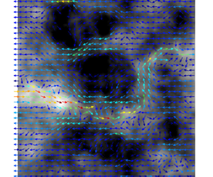

1. Introduction
Due to their formation history and to later tectonic constraints, the igneous rocks of the Earth's crust are heavily fractured (Bour & Davy Reference Bour and Davy1997; Renard & Allard Reference Renard and Allard2013). The resulting networks of interconnected fractures exhibit dimensions of fractures/cracks ranging from a few  $\mathrm {\mu }$m to several km for large-scale faults (Brown Reference Brown1987; Brown & Bruhn Reference Brown and Bruhn1998; Bonnet et al. Reference Bonnet, Bour, Odling, Davy, Main, Cowie and Berkowitz2001; Berkowitz Reference Berkowitz2002). Due to the very low permeability of the surrounding rock matrix, these fracture networks play a key role in the transport of water through the Earth's crust, with important implications on transport processes in the subsurface (Brantley, Goldhaber & Ragnarsdottir Reference Brantley, Goldhaber and Ragnarsdottir2007). The hydraulic transport characteristics of fractured rocks are thus of great importance for a broad range of environmental processes and subsurface applications, ranging from the petroleum industry to hydrogeology (Brown Reference Brown1987; Javadi, Sharifzadeh & Shahriar Reference Javadi, Sharifzadeh and Shahriar2010; Bense et al. Reference Bense, Gleeson, Loveless, Bour and Scibek2013) through contaminant transport in the subsurface (Grisak & Pickens Reference Grisak and Pickens1980; Roux, Plouraboué & Hulin Reference Roux, Plouraboué and Hulin1998; Detwiler, Rajaram & Glass Reference Detwiler, Rajaram and Glass2000; MacQuarrie & Mayer Reference MacQuarrie and Mayer2005), geothermal energy (Ledésert et al. Reference Ledésert, Hebert, Genter, Bartier, Clauer and Grall2010) and the storage of radioactive waste in subsurface repositories (Bredehoeft et al. Reference Bredehoeft, England, Stewart, Trask and Winograd1978; de La Vaissière, Armand & Talandier Reference de La Vaissière, Armand and Talandier2015), among other important applications.
The hydraulic behaviour of fractured rocks is controlled both by the topology of the networks of interconnected fractures (Long, Gilmour & Witherspoon Reference Long, Gilmour and Witherspoon1985; de Dreuzy, Davy & Bour Reference de Dreuzy, Davy and Bour2001, Reference de Dreuzy, Davy and Bour2002; Painter & Cvetkovic Reference Painter and Cvetkovic2005) and by the roughness of fracture walls, which impacts the hydraulic response of each individual fracture (Brown Reference Brown1987) in the network. Under particular conditions, considering fracture wall roughness in the flow description results in changing the connectivity of flow at the network scale (de Dreuzy, Méheust & Pichot Reference de Dreuzy, Méheust and Pichot2012), which indicates a coupling between fracture-scale flow complexity and network-scale flow connectivity. However, in most cases, and in particular when considering flow domains of sufficiently large scale in natural fractured porous media, these two contributions to the medium permeability are mutiplicative (de Dreuzy et al. Reference de Dreuzy, Méheust and Pichot2012), and can be studied separately. Many studies have thus addressed the fracture-scale contribution, i.e. the hydraulic behaviour of individual rough fractures. Such studies, which include laboratory-scale experiments (Yeo, De Freitas & Zimmerman Reference Yeo, De Freitas and Zimmerman1998; Méheust & Schmittbuhl Reference Méheust and Schmittbuhl2000; Wendland & Himmelsbach Reference Wendland and Himmelsbach2002; Konzuk & Kueper Reference Konzuk and Kueper2004; Molinero & Samper Reference Molinero and Samper2006; Watanabe, Hirano & Tsuchiya Reference Watanabe, Hirano and Tsuchiya2008) and theoretical/numerical investigations (Neuzil & Tracy Reference Neuzil and Tracy1981; Wong, Koplik & Tomanic Reference Wong, Koplik and Tomanic1984; Brown & Scholz Reference Brown and Scholz1985; Brown Reference Brown1987, Reference Brown1989; Tanksley & Koplik Reference Tanksley and Koplik1994; Brown Reference Brown1995; Brown & Bruhn Reference Brown and Bruhn1998; Rojas & Koplik Reference Rojas and Koplik1998; Drazer & Koplik Reference Drazer and Koplik2000; Méheust & Schmittbuhl Reference Méheust and Schmittbuhl2001; Drazer & Koplik Reference Drazer and Koplik2002; Bogdanov et al. Reference Bogdanov, Mourzenko, Thovert and Adler2003; Méheust & Schmittbuhl Reference Méheust and Schmittbuhl2003; Yan & Koplik Reference Yan and Koplik2008), have characterized the flow heterogeneity within rough walled fractures as a function of closure, and how that heterogeneity alters the transmissivity at the fracture scale.
Almost all of these studies have focused on pressure-driven flows, i.e. flows imposed by an externally maintained pressure drop along a given direction while the fracture is assumed to be closed in the transverse direction, with no consideration of solute transport (Brown Reference Brown1987; Zimmerman & Bodvarsson Reference Zimmerman and Bodvarsson1996; Nicholl et al. Reference Nicholl, Rajaram, Glass and Detwiler1999; Méheust & Schmittbuhl Reference Méheust and Schmittbuhl2001, Reference Méheust and Schmittbuhl2003; Basha & El-Asmar Reference Basha and El-Asmar2003; Brush & Thomson Reference Brush and Thomson2003; Koyama, Neretnieks & Jing Reference Koyama, Neretnieks and Jing2008; Wang et al. Reference Wang, Cardenas, Slottke, Ketcham and Sharp2015b). Others have also investigated solute transport, but without any feedback on the flow itself from the transport of ions (Drazer & Koplik Reference Drazer and Koplik2002; Cardenas et al. Reference Cardenas, Slottke, Ketcham and Sharp2007). However, fluid flow and the transport of ions (electrical charges) in solution are in fact expected to be coupled when their spatial distribution becomes heterogeneous (which can be enforced externally) due to the existence of electrical double layers (EDLs), which are essentially regions in the fluid containing net positive or negative charges (in the form of an ion) and located in the immediate vicinity ( ${\sim }O(1\text {--}100\,\text {nm})$) of mineral–water interfaces. Electrical double layers (Saville Reference Saville1977; Teutli-León et al. Reference Teutli-León, Oropeza, González and Soria2005; Hunter Reference Hunter2013) exist because rock surfaces, generally composed of minerals such as quartz (Pettijohn Reference Pettijohn1957; O'Connor et al. Reference O'connor1965) or kaolinite (López et al. Reference López, Bauluz, Fernández-Nieto and Oliete2005), usually posses a net electrical charge, which is either structural or results from chemical reactions with aqueous electrolytic solutions. For instance, silica, depending on the pH of the solution may undergo protonation or, de-protonation (Wang & Revil Reference Wang and Revil2010), which results in either positively or negatively charged mineral surfaces. Moreover, since natural pressure-driven flows can be very weak in fractures (Méheust & Schmittbuhl Reference Méheust and Schmittbuhl2000; Konzuk & Kueper Reference Konzuk and Kueper2004), the motion actuated by the interactions between EDLs and externally applied electric fields are expected to significantly alter the flow patterns therein. Consequently, analysis of the role of EDLs in subsurface porous media has far-ranging applications in geo-electrical measurements aiming at characterizing the shallow subsurface transport processes occurring in it (Revil et al. Reference Revil, Schwaeger, Cathles and Manhardt1999; Revil & Florsch Reference Revil and Florsch2010; Jougnot & Linde Reference Jougnot and Linde2013). More generally, interactions between EDLs and external electric fields, known as electrokinetic phenomena, also entail important applications in various systems of practical interest such as electrophoresis, particle separation, mixing of reagents, etc. (Squires & Quake Reference Squires and Quake2005; Hunter Reference Hunter2013). Furthermore, if a fracture is connecting two reservoirs with different concentrations of dissolved salts, the natural concentration gradient would then drive its own flow through the EDLs. This component of the flow, often termed diffuso-osmotic flow, might oppose or aid any existing mechanical (i.e. pressure-induced) flow, as well as any electrokinetic flow (Khair & Squires Reference Khair and Squires2008; Ghosh, Mandal & Chakraborty Reference Ghosh, Mandal and Chakraborty2017), and, hence, might also play a key role in altering the net throughput in the fracture. In addition, concentration gradients are expected to dictate the fluxes of charged solute species (and, thus, of electrical charges) through the fracture, thus triggering changes in the electrical current and, hence, in the overall electrical conductivity of the fracture. In this study we address the entire complexity of electrohydrodynamic couplings associated to rough fracture flow.
An approach commonly used to model rough fracture flow without electrohydrodynamical couplings is to use the lubrication approximation (Brown Reference Brown1987; Thompson Reference Thompson1991; Zimmerman, Kumar & Bodvarsson Reference Zimmerman, Kumar and Bodvarsson1991), which assumes slow spatial variations of the aperture field and allows deriving the Reynolds equation for the pressure field. In this depth-averaged formalism, pressure only varies along the two-dimensional (2-D) fracture's mean plane, while the fluid mass flux (also independent of the out-of-plane coordinate) depends on the local pressure gradient in a way akin to Darcy's law. Despite the constraint imposed on the geometry by the lubrication approximation, Brown and coworkers (Brown Reference Brown1987; Brown, Stockman & Reeves Reference Brown, Stockman and Reeves1995) have shown that high spatial frequency modes of the aperture field only play a minor role in dictating the fracture's transmissivity, which makes the Reynolds equation a reasonable approach to investigate the global features of flow through fractures, as evident from the good agreement between fracture hydraulic apertures (Brown Reference Brown1989; Méheust & Schmittbuhl Reference Méheust and Schmittbuhl2001) computed from the Reynolds equation and measured from laboratory experiments (Mourzenko, Thovert & Adler Reference Mourzenko, Thovert and Adler1995; Nicholl et al. Reference Nicholl, Rajaram, Glass and Detwiler1999; Méheust & Schmittbuhl Reference Méheust and Schmittbuhl2000; Konzuk & Kueper Reference Konzuk and Kueper2004). On the other hand, several researchers have investigated flow through fractures by solving the three-dimensional (3-D) Stokes equation using various computational tools (Mourzenko et al. Reference Mourzenko, Thovert and Adler1995; Rojas & Koplik Reference Rojas and Koplik1998; Cardenas et al. Reference Cardenas, Slottke, Ketcham and Sharp2007) and concluded that the lubrication theory-based analysis remains reasonably accurate provided that the surface roughness’ standard deviation is sufficiently small, but that solving the 3-D flow is more accurate. Note, however, that solving the flow from the 2-D Reynolds equation is considerably faster and allows for Monte-Carlo studies over a large statistics of fractures with identical geometric parameters but possibly significantly different transmissivities, due to the intrinsically stochastic nature of these objects (Méheust & Schmittbuhl Reference Méheust and Schmittbuhl2001). Be that as it may, all aforementioned studies only consider purely pressure-driven flows, and only a handful of them have investigated electrical transport through fractures (Tsang Reference Tsang1984; Brown Reference Brown1989; Thompson & Brown Reference Thompson and Brown1991); they have done so by treating hydrodynamics and electromechanics as independent phenomena.
Although the electrokinetic effects discussed above are likely to be negligible in fractures with mean apertures in the millimetre range (Hamzehpour et al. Reference Hamzehpour, Atakhani, Gupta and Sahimi2014), the effect of the EDL can become significant (Marino et al. Reference Marino, Coelho, Bekri and Adler2000; Hamzehpour et al. Reference Hamzehpour, Atakhani, Gupta and Sahimi2014) when the mean aperture is in the range 10–100  $\mathrm {\mu }$m or less (the upper value of which being very common in subsurface fractured media, in particular). Such microfractures play key roles in oil and gas recovery (Gamson, Beamish & Johnson Reference Gamson, Beamish and Johnson1993), dictating the physical properties of rocks, and playing a particular role in rock failure and the development of fault zones (Anders, Laubach & Scholz Reference Anders, Laubach and Scholz2014). More generally, EDLs and the associated ionic gradients play important roles in dictating various properties of the subsurface such as direct current and complex conductivity (also called induced polarization) (Marshall & Madden Reference Marshall and Madden1959; Kessouri et al. Reference Kessouri2019) and streaming potential (Linde et al. Reference Linde, Jougnot, Revil, Matthäi, Arora, Renard and Doussan2007; Revil et al. Reference Revil, Linde, Cerepi, Jougnot, Matthäi and Finsterle2007), which may be used to map the structure of underground porous media, the saturation of fluid phases in them, the spatial distribution of a contaminant plume in the subsurface, or the activity of bacteria therein. Despite this, the impacts of concentration gradients and of the presence of EDLs on overall transport phenomena in rough fractures have remained largely unexplored, to the best of our knowledge. In particular, detailed exploration of electro-osmotic flow triggered by EDLs are so far lacking in the literature, with the notable exception of the studies by Marino et al. (Reference Marino, Coelho, Bekri and Adler2000), who have developed 3-D numerical simulations for coupled mechanical and electro-osmotic flow in rough fractures based on first principle equations. They investigated in particular the influence of the self-affinity of the fracture wall roughness and its amplitude on the coupling between the two phenomena, albeit in the limit of small deviations from equilibrium conditions. To theoretically describe the first principles of electrohydrodynamics, the Poisson–Nernst–Planck–Navier–Stokes (PNPNS) equations are a well-established formulation (Saville Reference Saville1977; Kilic, Bazant & Ajdari Reference Kilic, Bazant and Ajdari2007; Schnitzer & Yariv Reference Schnitzer and Yariv2012; Schmuck & Bazant Reference Schmuck and Bazant2015; Ghosh, Chaudhury & Chakraborty Reference Ghosh, Chaudhury and Chakraborty2016; Ghosh et al. Reference Ghosh, Mandal and Chakraborty2017), although more advanced models exist (Bazant et al. Reference Bazant, Kilic, Storey and Ajdari2009) to address configurations for which either the potentials are very large, the ion concentrations are very large or the dimensions of the confining space are very small; such configurations however, are outside the scope of this study. Resorting to numerical modelling of the PNPNS equations in the 3-D space of the fracture nevertheless has several drawbacks. Firstly, it is computationally very expensive, and, hence, would not allow studying a large number of fracture realizations for a given set of geometrical parameters. Studies of Stokes flow in geological rough fractures have shown that large fluctuations can exist within such statistics, and that any conclusion that claims a certain level of universality must be obtained from a sufficient statistics of fractures with identical statistical geometrical parameters (Méheust & Schmittbuhl Reference Méheust and Schmittbuhl2001, Reference Méheust and Schmittbuhl2003). Secondly and more fundamentally, a full 3-D model requires the EDL to be finely resolved for accurate computations. This is very difficult from a practical point of view, as the EDL size is typically of a few nms to a few hundreds of nm, and the fracture aperture can be as large as 1 mm.
We propose here a general theoretical model to address fully coupled electrohydrodynamical transport through rough fractures in the two dimensions of a fracture plane, based on the lubrication approximation. Although a handful of previous studies (Park et al. Reference Park, Russo, Branton and Stone2006; Ghosal Reference Ghosal2002, Reference Ghosal2003; Datta & Ghosal Reference Datta and Ghosal2009) have extended the lubrication theory to electrokinetic flows, most of them only concentrate on the consequences of the electrical effects on the Navier–Stokes equations. While these approaches conserve the fluid mass flow rate, they do not conserve the electrical current and salt fluxes; to ensure their conservation, additional constraints are required to complement the Reynolds equation. In the present study we thus derive a generalization of the Reynolds equation accounting for the coupled transport of fluid mass, electrolytes and electrical charges in the space between two rough walls which possess a surfacic spatial distribution of charges. Our generalized framework brings out the intricate coupling between liquid motion, current and salt flux in a rough narrow fracture, a physical paradigm that currently remains mostly unexplored in the literature. The flow is actuated using a combination of externally prescribed electrical potential, concentration difference and pressure difference. This generalized lubrication theory is thoroughly validated by comparing its predictions with the results of 3-D numerical resolutions of the PNPNS equations in small-size realizations of synthetic geological (rough) fractures. We subsequently apply the generalized theory to investigate coupled flow and ion transport through large-size geological fractures whose walls bear surface charge and which are subjected to prescribed pressure, potential and concentration differences between their inlet and outlet.
The geometry considered and the assumptions of the model are presented in § 2, and the first principle equations in § 3. Section 4 is dedicated to the development of the equations describing the general lubrication theory. The significance of our general formalism with respect to the existing literature, linking the lubrication theory and electrohydrodynamics is also outlined in that section. The validation of the model and the results obtained from applying the model to synthetic geological fractures are presented and discussed in § 5. Section 6 is the conclusion. Appendix A presents details on the derivation of the coupled conservation equations, while Appendix B shows additional comparative tests for the model. Analytical solutions to the generalized equations for special cases of fracture aperture geometries that are invariant along one direction, as well as additional validations of the lubrication-based model predicated on comparisons with those analytical solutions and with numerical simulations of the PNPNS equations in 3-D and 2-D test (non-stochastic) geometries are presented in §§ S2, S5 and S6 of the supplementary material available at https://doi.org/10.1017/jfm.2022.306, while § S3 therein compares results from our general lubrication theory to those from an earlier theoretical model with a lesser level of generality.
2. Geometry considered and assumptions of the model
2.1. Geometry of the fracture
Measurements of fracture surface topographies demonstrate that they exhibit a roughness possessing long-range spatial correlations and a scale invariance characteristic of self-affinity (Schmittbuhl, Schmitt & Scholz Reference Schmittbuhl, Schmitt and Scholz1995). This means that the height distribution  $h'(x',y')$ of an isotropic fracture surface, such as the fracture walls shown in figure 1, has the following scale invariance property:
 \begin{equation} \lambda^{H}f(\lambda^{H}\Delta h',\lambda r') = f(\Delta h',r'). \end{equation}
Here  $f(\Delta h',r')$ is the probability density function (p.d.f.) of having a height difference
 $\Delta h'$ between two points belonging to the topography and separated by a horizontal distance
 $r'=\sqrt {(\Delta x')^2 + (\Delta y')^2}$, and
 $H$ denotes the Hurst exponent (Bouchaud, Lapasset & Planès Reference Bouchaud, Lapasset and Planès1990). Except for materials such as sandstone for which fracturing occurs in-between mineral grains (Boffa, Allain & Hulin Reference Boffa, Allain and Hulin1998), the value of the Hurst exponent has been measured to
 $0.8$ for a large range of different materials and length scales (Bouchaud et al. Reference Bouchaud, Lapasset and Planès1990); this value shall be used here. In addition, the p.d.f. in (2.1) has been measured to be Gaussian (Brown Reference Brown1995). Self-affinity imparts long-range correlations to the topography, which means that if the topography is isotropic, its autocorrelation function
 \begin{equation} \mathcal{C}(\Delta x',\Delta y') = \frac{1}{L'_x L'_y}\int_{0}^{L'x} \,{{\rm d} x}' \int_{0}^{L'_y} \,{{\rm d} y}' h'\left(x',y'\right)h'\left(x'+\Delta x',z'+\Delta y'\right) \end{equation}
is a function of  $r'$ alone, and
 $C(0)-C(r')$ scales as a power law
 $r'^{2H}$ (Schmittbuhl et al. Reference Schmittbuhl, Schmitt and Scholz1995). Consequently, the power spectral density (PSD)
 $G(k')$, which is defined for an isotropic fracture as (Wang, Narasimhan & Scholz Reference Wang, Narasimhan and Scholz1988; Brown Reference Brown1995; Schmittbuhl et al. Reference Schmittbuhl, Schmitt and Scholz1995)
 \begin{equation} G(k') = \frac{1}{2{\rm \pi}}\int_{-\infty}^{\infty} \mathcal{C}(r') {\rm e}^{-{\rm i}k'r'}\, {\rm d}r' , \end{equation}
scales as  $k'^{-2(H+1)}$.
A synthetic single fracture with self-affine walls of Hurst exponent  $0.8$ connects two reservoirs along the
 $x'$-axis. The aperture field
 $a'(x',y')$ has a mean
 $a'_{m} = 100\,\mathrm {\mu }$m and standard deviation
 $\sigma ' = 0.9\,a'_{m}$. The correlation length is
 $L_{c}= L'_x/2 = 10^3 a'_{m} = 10$ cm. The fracture is closed along its lateral boundaries (defined by
 $y'=0$ and
 $y'=L'_y$). The walls carry a surface charge distribution, represented by an equivalent zeta potential
 $\zeta '(x',y')$. The outlet and the inlet are subjected to different levels of pressure, concentration and electrical potential.

The two walls constituting a fracture possess the same self-affinity property, with identical Hurst exponent and standard deviation of  $h'(x',z')$. The aperture field is defined as
 \begin{align} \left. \begin{array}{ll@{}} a'(x',y')= \max\left (h'_{t}(x',y') - h'_{b}(x',y')+a'_{m},0 \right) & \text{if } h'_{t}(x',y') + a'_{m} > h'_{b}(x',y'), \\ a'(x',y') = 0 & \text{otherwise}, \end{array} \right\} \end{align}
where the topographies for the upper and the lower walls,  $h'_{t}$ and
 $h'_{b}$, are defined with a zero arithmetic mean and
 $a'_{m}$ is the fracture's mechanical aperture, which is the distance between the mean planes of the walls and is also the arithmetic mean of the aperture field
 $a'$ when the two fracture walls are not touching each other. At
 $(x,y)$ positions where
 $h'_{t}(x',y') - h'_{b}(x',y')+a'_{m}$ is negative, meaning that the two original wall topographies intersect each other, the aperture is set to zero, which is equivalent to considering perfect plastic closure of the fracture. Fracture walls pertaining to a freshly made fracture are identical down to very small scales, yielding
 $h'_{t}=h'_{b}$ and a constant aperture
 $a'(x,y)=a'_{m}\,\forall (x,y)$. But the walls of a geological fracture are only identical at scales larger than a characteristic correlation scale
 $L_{c}$. Below that scale they are both self-affine but uncorrelated to each other, so the aperture field is also self-affine (since self-affinity is a linear property). The PSD of the aperture field is then of the form
 \begin{equation} \left. \begin{array}{ll@{}} G(k') \propto ({k'_x}^2+{k'_y}^2)^{-(H+1)} & \text{if } \sqrt{{k'_x}^2+{k'_y}^2}\leq k'_{c}=\dfrac{\rm \pi}{L_{c}}, \\ G(k') = G(k'_{c}) & \text{otherwise}. \end{array} \right\} \end{equation}
Consequently, the aperture field of a geological fracture is well modelled as a stationary 2-D random process (Brown Reference Brown1995) defined by (i) the functional form of the p.d.f. for  $a'$ – this includes specification of the mean
 $a'_{m}$ and standard deviation
 $\sigma$; (ii) the Hurst exponent
 $H$; (iii) the correlation length
 $L_{c}$; and (iv) the horizontal dimensions
 $L'_x$ (length) and
 $L'_y$ (width) of the fracture (Méheust & Schmittbuhl Reference Méheust and Schmittbuhl2003). The synthetic fractures of § 5.2 have been generated using a spectral method previously employed by Méheust & Schmittbuhl (Reference Méheust and Schmittbuhl2001, Reference Méheust and Schmittbuhl2003). The perfect plastic closure in contact zones, expressed by the notation
 $\max (\cdot, 0)$ in (2.4), is the strongest approximation made in this model of geological fracture.
2.2. Boundary conditions and assumptions of the model
We consider steady coupled Stokes flow and ion/charge transport through a synthetic fracture as shown in figure 1. The  $x'$ and
 $y'$ axes run along the mean fracture plane, while the
 $z'$-axis is normal to that plane, hence running along the fracture's aperture. The top (respectively, bottom) surface has a surface charge density
 $q'_{t}(x',y')$ (respectively,
 $q'_{b}(x',y')$), which for the moment is considered to be an arbitrary function of
 $x'$ and
 $y'$. We assume that the fracture connects two reservoirs along the
 $x$-axis which contain solutions of the same
 $1:1$ symmetrical electrolyte, of respective concentrations
 $c'_{in}$ and
 $c'_{ex}$. A solution of the same electrolyte also saturates the fracture. The pressures at the inlet and outlet are maintained at
 $p'_{in}$ and
 $p'_{ex}$, respectively, while the electrical potential difference imposed between the two reservoirs is
 $\Delta V$. We further assume that there is no externally imposed electrical potential difference between the two fracture walls, as such a potential difference would not impact the flow and ion transport in the fracture. We further assume that the faces of the fracture lying perpendicular to the
 $y'$-axis, at
 $y'=0$ and
 $y'=L'_y$, are closed. The presence of surface charge on the fracture walls and electrolyte solution inside the fracture leads to the formation of EDLs in the vicinity of the walls. We assume that the EDLs are non-overlapping, so that for any
 $(x_0,y_0)$ position along the mean fracture plane, the region away from either of the walls lying on the line segment
 $(x=x_0,y=y_0)$ remains electroneutral. The fluid viscosity is denoted
 $\eta$, its density
 $\rho _f$ and the liquid's electrical permittivity
 $\gamma$. All these properties are assumed to remain constant throughout.
We present in the following a formulation for coupled fluid and charge transport in a fracture geometry based on the lubrication approximation. This model makes the following several assumptions.
(i) The topography varies slowly as a function of the horizontal coordinates, i.e.
 $\forall (x,y), \| \boldsymbol {\nabla } a \| \ll 1$. Note that the aperture field's self-affinity implies that the aperture gradient goes to infinity when computed over a vanishingly small horizontal length scale (see Méheust & Schmittbuhl Reference Méheust and Schmittbuhl2001); therefore, depending on the size of the computing mesh, the aperture topography may have to be smoothed below a length scale $\ell _c$ such that $\varepsilon = \Delta a_0 / \ell _c \ll 1$, where $\Delta a_0$ is the typical vertical variation in the aperture field over $\ell _c$, so as to ensure that the lubrication approximation be valid. However, Brown (Brown Reference Brown1987; Brown et al. Reference Brown, Stockman and Reeves1995) has shown that small wavelength features of the surface roughness only play a secondary role in controlling the flow heterogeneity at the fracture scale, so, if $\ell _c \ll L_{c}$, transport processes at the fracture scale will not be significantly impacted by this small-scale smoothing of the aperture field. The validity of the lubrication approximation will be verified by comparing the results of the lubrication-based model to the numerical solutions of the first principle equations in identical geometrical and electrical configurations in § 5.1.
(ii) For the sake of generality, we assume the surface charge to be variable as well, but its gradient is also much smaller than 1, which means that the characteristic length scales of variation
$l_0$ (say) of the surface charges are of same order as those of the topography ($l_0\sim L_c$).(iii) The Reynolds number is assumed to be small (
$Re\ll 1$), which is a reasonable assumption for most configurations of fracture flow in the subsurface.(iv) We assume that the magnitude of the surface charge and potential gradient imposed across the fracture are not asymptotically large (see details in § 4.1).
(v) Finally, since the theory is derived from the Poisson–Nernst–Planck equations, the usual assumptions are made for these equations (for example, point charges, no non-Coulombic interactions between ions, etc.). Although several modifications to the Nernst–Planck equations have been proposed (Bazant et al. Reference Bazant, Kilic, Storey and Ajdari2009), the Nernst–Planck equations are capable of capturing the essential physics with a reasonable accuracy, especially when investigating effective transport characteristics in subsurface permeable media (see § 5.2).


Since we are applying the lubrication theory, conditions for primitive variables (e.g. velocity) are not required at the flow domain boundaries. However, boundary conditions for the externally imposed potential ( $\phi '$), concentrations and pressure are required to close the system of governing equations, as we show later. These conditions are given by
 \begin{align} & \text{At}\quad x' = 0, \quad p'=p'_{in};\quad c'_i=c_{in};\quad \phi'=0, \end{align}
 \begin{align} & \text{At}\quad x' = L'_x, \quad p'=p'_{ex};\quad c'_i=c_{ex};\quad \phi'={-}\Delta V, \end{align}
 \begin{align} & \text{At}\quad y' = 0 \ \text{and}\ L'_y \quad \partial p'/\partial y'= \partial c'_{{\pm}}/\partial y'= \partial \phi'/\partial y' = 0. \end{align}
The last condition expresses the constraint that the diffusive fluxes of pressure, solute concentration and electrical potential, have no component along the  $y'$-axis at the lateral boundaries of the fracture.
Note that the generalized lubrication equations derived in the following assume no specific relation between  $h'_b$ and
 $h'_t$; thus, they remain valid for symmetric fractures (i.e. with wall topographies that mirror each other) as well as non-symmetric fractures. As we shall show below, the only required geometrical input to the generalized lubrication equations is the aperture field.
3. The first principle governing equations
The PNPNS equations govern the flow and charge transport in the fracture. These equations may be written as (Saville Reference Saville1977)
 $$\begin{gather} \boldsymbol{v'}\boldsymbol{\cdot}\boldsymbol{\nabla}' c'_{+} =D\nabla'^2c'_{+}+\frac{eD}{k_{b} T}\boldsymbol{\nabla}'\boldsymbol{\cdot}\{c'_{+}\boldsymbol{\nabla}' \psi'\}, \end{gather}$$
 $$\begin{gather}\boldsymbol{v'}\boldsymbol{\cdot}\boldsymbol{\nabla}' c'_{-} =D\nabla'^2c'_{-}-\frac{eD}{k_{b} T}\boldsymbol{\nabla}'\boldsymbol{\cdot}\{c'_{-}\boldsymbol{\nabla}' \psi'\}, \end{gather}$$
 $$\begin{gather}\nabla'^2\psi' ={-}(c'_{+}-c'_{-})/\gamma, \end{gather}$$
 $$\begin{gather}0={-}\boldsymbol{\nabla}' p' +\eta\boldsymbol{\nabla}'^2\boldsymbol{v'}+\gamma\nabla'^2\psi'\boldsymbol{\nabla}'\psi'; \quad\boldsymbol{\nabla}'\boldsymbol{\cdot}\boldsymbol{v'} = 0 . \end{gather}$$
In these equations  $\psi '$ is the total electrostatic potential field,
 $c'_{+}$ and
 $c'_{-}$ are respectively the concentration fields for the positively and negatively charged ions,
 $\boldsymbol {v'}$ is the fluid velocity field and
 $p'$ is the pressure field. The parameters
 $D$,
 $e$,
 $k_{b}\simeq 1.38\times 10^{-23}$ J K
 $^{-1}$ and
 $T$ are respectively the molecular diffusion coefficient, the protonic charge, the Boltzmann constant and the absolute temperature. The boundary conditions at the inlet and outlet of the fracture have already been presented in (2.6a)–(2.6c), whereas the conditions on the fracture walls read as
 \begin{equation} \boldsymbol{j'}_{{\pm}}\boldsymbol{\cdot}\boldsymbol{n}_k = \boldsymbol{v'} = 0;\quad \boldsymbol{\nabla}'\psi'\boldsymbol{\cdot}\boldsymbol{n}_k ={-}\frac{q'_k(x',y')}{\gamma}, \end{equation}
where,  $\boldsymbol {j}_{\pm } = \boldsymbol {v'}c'_{\pm }-D\boldsymbol {\nabla }'c'_{\pm }\mp (k_{b} T)^{-1}eDc'_{\pm }\boldsymbol {\nabla }'\psi '$ is the flux of the positively (respectively negatively)-charged ions;
 $k \equiv \{t,\;b\}$ indicates either the top or the bottom wall and
 $\boldsymbol {n}$ is the unit vector normal to the wall. The boundary conditions in (3.2a,b) basically indicate that the fracture walls are impermeable to ions, while the fluid satisfies the no-slip and no-penetration boundary conditions. For readers who are familiar with fracture flow in the subsurface but not with electrohydrodynamics, we present in § S1 of the supplementary material a brief derivation of (3.1) from the Stokes (flow) equation, Nernst–Planck (transport) equation and Poisson equation (link between electrical field and volumetric charge density).
It is convenient to work with the dimensionless versions of the above equations. To this end, we represent the non-dimensional version of any variable (say,  $\xi '$) as follows:
 $\xi _* = \xi '/\xi _{c}$, where the generic variable
 $\xi '$ represents a quantity such as
 $u',v', p', \phi ',\ldots$, etc., and
 $\xi _{c}$ is the characteristic scale for that quantity. Table 1 provides these scale definitions, wherein the characteristic velocity u
 $_{c}$ has been defined assuming that pressure gradients are the dominant actuating force.
Characteristic (Char.) scales chosen to non-dimensionalize the PNPNS equations and the equations expressing the associated boundary conditions.

We further express the Nernst–Planck equations in terms of total non-dimensional salt concentration ( $c_*$) and charge density (
 $\rho _*$), defined as follows:
 $c_*=c_{+,*}+c_{-,*}$ and
 $\rho _* = c_{+,*}-c_{-,*}$. The corresponding non-dimensional charge and salt fluxes are then
 $\boldsymbol {i}_* = \boldsymbol {j}_{+,*}-\boldsymbol {j}_{-,*}$ and
 $\boldsymbol {j}_* = \boldsymbol {j}_{+,*}+\boldsymbol {j}_{-,*}$, respectively. Finally, to render the implementation of the relevant boundary conditions easier, we split the electrostatic potential (
 $\psi _*$) into two contributions: (i) the one from the externally imposed potential difference,
 $\phi _*$, and (ii) the potential resulting from the presence of the EDL,
 $\varphi _*$; therefore,
 $\psi _* = \phi _* + \varphi _*$. The non-dimensional fluxes are then related to the primitive variables as follows:
 $$\begin{gather} \boldsymbol{i}_* = \rho_* \boldsymbol{v}_*-Pe^{{-}1}\boldsymbol{\nabla}_*\rho_*-Pe^{{-}1}c_*\boldsymbol{\nabla}_*(\varphi_*+\phi_*), \end{gather}$$
 $$\begin{gather}\boldsymbol{j}_* = c_* \boldsymbol{v}_*-Pe^{{-}1}\boldsymbol{\nabla}_* c_*-Pe^{{-}1}\rho_*\boldsymbol{\nabla}_*(\varphi_*+\phi_*). \end{gather}$$
Here  $Pe=u_{c}l_0/D$ is the ionic Péclet number, which is usually
 $O(1)$ for field driven flows (Saville Reference Saville1977), although it can be larger when flows are externally imposed. After enforcing the aforementioned non-dimensionalization scheme, the PNPNS equations take the form
 $$\begin{gather} \boldsymbol{\nabla}_*\boldsymbol{\cdot}\boldsymbol{i}_* = \boldsymbol{\nabla}_*\boldsymbol{\cdot}\boldsymbol{j}_* = 0, \end{gather}$$
 $$\begin{gather}\nabla_*^2\varphi_* ={-}\frac{1}{2}\kappa_*^2\rho_*\ \text{and}\ \nabla_*^2\phi_*=0, \end{gather}$$
 $$\begin{gather}0={-}\boldsymbol{\nabla}_* p_* +\boldsymbol{\nabla}_*^2\boldsymbol{v}_*+\alpha\nabla_*^2\varphi_*\boldsymbol{\nabla}_*(\varphi_*+\phi_*) \quad \text{and} \quad\boldsymbol{\nabla}_*\boldsymbol{\cdot}\boldsymbol{v}_* = 0, \end{gather}$$
where additional non-dimensional parameters are defined as (i) the ratio of the characteristic length scale to the Debye screening length,  $\kappa _*^2 = 2c'_{in}e^2l^2_0/(\gamma k_{b}T)$, and (ii)
 $\alpha = u_{ek}/u_{c}$. Note also that the Reynolds number,
 $Re=\rho _{f} u_{c}l_0/\eta$, does not appear in the non-dimensional equations due to the assumption of creeping flow (
 $Re\ll 1$). The boundary conditions for the above equations at the
 $k$th wall are given by
 \begin{equation} \boldsymbol{j}_*\boldsymbol{\cdot}\boldsymbol{n}_k=\boldsymbol{i}_*\boldsymbol{\cdot}\boldsymbol{n}_k=0;\quad\boldsymbol{\nabla}_*\varphi_*\boldsymbol{\cdot}\boldsymbol{n}_k={-}q_{k,*}(x_*,y_*)\quad \text{and}\quad\boldsymbol{v}_* = 0 , \end{equation}
 $q_{k,*}$ being the non-dimensional surfacic charge density field. Note that the velocity satisfies the no-slip condition at the fracture walls, because the continuum hypothesis remains valid everywhere in the fracture. Indeed, the typical mean aperture of most fractures (Gamson et al. Reference Gamson, Beamish and Johnson1993) is significantly larger than
 $1\,\mathrm {\mu }$m, so that the Knudsen number
 $= \lambda _{{mfp}}/a'_{{m}}$, where
 $\lambda _{{mfp}} \sim 10^{-8}$ m is the molecular mean free path (Karniadakis, Beskok & Aluru Reference Karniadakis, Beskok and Aluru2006), remains well below 0.01. It could exceed this value locally in regions of very low aperture (
 $<10$ nm) close to the contact zones, but the in-plane extent of such regions around the contact zones can be estimated to approximately 10 nm as well. Thus, their size is small in comparison to the fracture size, so that these regions hardly impact the coupled flow and transport process; in addition, they are too small to be resolved by any mesh which may be used on fractures of even centimetric in-plane dimensions. Hence, implementing the Navier slip condition (Karniadakis et al. Reference Karniadakis, Beskok and Aluru2006) in such regions is not necessary.
The boundary conditions for pressure, concentration and potential ( $\phi$) at the two ends of the fracture (refer to conditions (2.6a)–(2.6c)) can be rewritten non-dimensionally in the following way, with
 $L_{x,*} = L'_x/l_0$,
 $L_{y,*} = L'_y/l_0$, and
 $\beta = e(\Delta V'/L'_x)l_0/(k_{b}T)$:
 \begin{align} & \text{At}\quad x_* = 0,\quad p_* = p_{in,*};\quad c_* = 1;\quad \phi_* = 0, \end{align}
 \begin{align} & \text{At}\quad x_* = L_{x,*},\;\;p_* = p_{ex,*},\quad c_* = c_{ex,*};\quad \phi_* ={-}\beta L_{x,*}, \end{align}
This constant, which is used to express the boundary condition for the potential (i.e. (3.6b)), is popularly known as the applied field strength, considered in comparison to the thermal potential (Saville Reference Saville1977). It can have a wide range of values. Usually,  $\beta \ll 1$ is referred to as the weak field limit (Saville Reference Saville1977), while
 $\beta \gg 1$ is the strong field limit (Schnitzer & Yariv Reference Schnitzer and Yariv2012).
4. Lubrication theory for the coupled transport problem
4.1. The rescaled equations
As already discussed, the essence of the theory states that (Brown Reference Brown1987; Leal Reference Leal2007): the typical length scale of variation of the relevant quantities (such as pressure, velocity, concentration, etc.) along the fracture plane is much larger than that across the fracture thickness. This may be summarized here as  $\varepsilon = h_0/l_0 \ll 1$ (Leal Reference Leal2007), where here
 $l_0$ can be the correlation length (
 $L_c$) and
 $h_0$ can be the mean aperture (
 $a_{{m}}$). Such a physical paradigm necessitates the following rescaling of the relevant variables and fluxes (Leal Reference Leal2007):
 $p_* = \varepsilon ^{-2}p$;
 $w_* = \varepsilon w$;
 $z_* = \varepsilon z$ and
 $\kappa _* = \varepsilon ^{-1}\kappa$, while the rest of the variables remain the same and their rescaled versions are also expressed without the subscript ‘
 $_*$.’ The purpose of the rescaling is essentially to make all the variables
 $\mathcal {O}(1)$ quantities.
Now, following the principles of the lubrication theory (Batchelor Reference Batchelor2000; Leal Reference Leal2007), we expand all the rescaled variables in a regular asymptotic series in  $\varepsilon$ as
 \begin{equation} \varTheta = \varTheta_0 + \varepsilon\varTheta_1+\varepsilon^2\varTheta_2 + \cdots, \end{equation}
where the  $\varTheta$ can represent quantities such as
 $u$,
 $v$, etc. We substitute the above asymptotic series into the rescaled governing equations and retain the leading-order terms in
 $\varepsilon$ to deduce the following:
 $$\begin{gather} \frac{\partial^2 \varphi}{\partial z^2} + \frac{1}{2}\kappa^2\rho = 0 \quad \text{and} \quad \frac{\partial^2 \phi}{\partial z^2} = 0, \end{gather}$$
 $$\begin{gather}\frac{\partial^2 c}{\partial z^2}+\frac{\partial}{\partial z}\left(\rho\frac{\partial \varphi}{\partial z}\right)=0\quad \text{and}\quad \frac{\partial^2 \rho}{\partial z^2}+\frac{\partial}{\partial z}\left(c\frac{\partial \varphi}{\partial z}\right)=0, \end{gather}$$
 $$\begin{gather}-\frac{\partial p}{\partial z} +\alpha\frac{\partial^2 \varphi}{\partial z^2}\frac{\partial \varphi}{\partial z}=0\quad \text{and}\quad {-}\boldsymbol{\nabla}_{H} p + \frac{\partial^2 \boldsymbol{v}_{H}}{\partial z^2}+\alpha\frac{\partial^2 \varphi}{\partial z^2}\boldsymbol{\nabla}_{H}\left(\varphi+\phi\right)=0, \end{gather}$$
 $$\begin{gather}\boldsymbol{\nabla}_{H}\boldsymbol{\cdot}\boldsymbol{v}_{H} + \frac{\partial w}{\partial z} = 0. \end{gather}$$
Here  $\boldsymbol {\nabla }_{H} \equiv \boldsymbol {\hat {e}}_x({\partial }/{\partial x})+\boldsymbol {\hat {e}}_y ({\partial }/{\partial y})$ and
 $\boldsymbol {v}_{H} = u\boldsymbol {\hat {e}}_x + v\boldsymbol {\hat {e}}_z$ are respectively the projection of the gradient operator onto the fracture plane and the velocity along that plane. In (4.2) we have made use of the fact that to leading order,
 $\phi$ is only a function of
 $x$ and
 $y$ (
 $\phi = \phi (x,y)$), as we shortly demonstrate. The equations are subject to the following boundary conditions, after application of the lubrication approximation. At
 $z= z_{t}(x,y) = -1/2+h_{b}(x,y)$ and
 $z = z_{b}(x,y) = 1/2+h_{t}(x,y)$,
 $$\begin{gather} \left[\frac{\partial c}{\partial z} + \rho\frac{\partial \varphi}{\partial z}\right] _{z=z_{{t}\vert{b}}} = \left[\frac{\partial \rho}{\partial z} + c\frac{\partial \varphi}{\partial z}\right] _{z=z_{{t}{b}}}= 0, \end{gather}$$
 $$\begin{gather}\varphi =\zeta_{t}(x,y)\quad\text{or}\quad\zeta_{b}(x,y);\quad \left(\frac{\partial \phi}{\partial z}\right)_{z=z_{{t}{b}}} = 0;\quad \text{and}\quad\boldsymbol{v} _{z=z_{{t}\vert{b}}}= 0. \end{gather}$$
Note that in (4.3b) the specified surface charge density condition from (3.5a–c) has been replaced by a Diritchlet boundary condition with a known potential (the zeta potential (Hunter Reference Hunter2013)) that defines the potential drop across the diffuse part of the EDL. It can be easily verified that these two forms are largely equivalent, since at leading order the EDL can effectively be considered at equilibrium (Hunter Reference Hunter2013; Ghosh et al. Reference Ghosh, Chaudhury and Chakraborty2016). We assume that  $\max \{\zeta \} \sim \mathcal {O}(1)$, i.e. the surface potential is not asymptotically large as compared with the thermal potential. The boundary conditions at
 $x=0$ and
 $x=L_x$ remain the same as given in (3.6).
The governing equations (4.2) can be solved semi-analytically. Based on (3.4b) and (4.3b), it is straightforward to establish that  $\phi$ does not depend on
 $z$ (
 $\phi = \phi (x,y)$). However, the functional form of
 $\phi (x,y)$ is not yet known and we elaborate on how to find this functional dependence in the next subsection. Solving the leading-order Nernst–Planck equations (4.2b) yields ionic concentrations that satisfy the Boltzmann distribution, which leads to (Kilic et al. Reference Kilic, Bazant and Ajdari2007)
 \begin{equation} c = 2\tilde{c}(x,y)\cosh (\varphi)\quad\text{and}\quad\rho ={-}2\tilde{c}(x,y)\sinh (\varphi) , \end{equation}
where  $\tilde {c}(x,y)$ is the bulk concentration of salt, assumed to remain neutral owing to non-overlapping EDLs; in general it will be a function of
 $x$ and
 $y$. This remains true even if there is no externally imposed concentration gradient along the fracture, as we demonstrate later on. Note that, just as
 $\phi (x,y)$,
 $\tilde {c}(x,y)$ is also an unknown and will be determined in the next subsection. The EDL potential (
 $\varphi$) then satisfies the Poisson–Boltzmann equation, given by
 \begin{equation} \frac{\partial^2 \varphi}{\partial z^2} = \kappa^2\tilde{c}(x,y)\sinh \varphi . \end{equation}
Note that this equation can be computed using a local vertical coordinate  $\tilde {z}$ obtained from
 $z$ through a translation such that
 $\tilde {z}=0$ at the bottom wall, and thus
 $\tilde {z} \in [0, a(x,y)]$. The equations expressing the associated boundary conditions, (4.3a) and (4.3b), are not impacted by this variable change, but the walls are located at
 $\tilde {z} = 0$ and
 $\tilde {z} =a(x,y)$ instead of
 $z_{{t}\vert {b}}$. Therefore, the distribution of
 $\varphi$ across the fracture only depends on the local aperture
 $a(x,y)$ and not on the particular pair of topographies
 $z_{{t}\vert {b}}$ that result in the aperture
 $a(x,y)$.
The  $z$-momentum equation in (4.2c) can then be solved for pressure to deduce
 \begin{equation} p = \alpha\kappa^2 \tilde{c}(x,y)\cosh (\varphi) + p_0(x,y) , \end{equation}
in which the first term, called the osmotic pressure, comes from the salt concentration in the fracture (Brunet & Ajdari Reference Brunet and Ajdari2004), and the second term ( $p_0(x,y)$) denotes the contributions from the induced pressure as well as the externally imposed pressure gradient. Similar to
 $\phi (x,y)$ and
 $\tilde {c}(x,y)$,
 $p_0(x,y)$ is yet to be determined and forms part of a closure problem. Inserting the pressure from (4.6) into the right-hand side equation in (4.2c), we obtain the following simplified form:
 \begin{equation} {-}\boldsymbol{\nabla}_{H} p_0-\alpha\kappa^2 \cosh (\varphi)\boldsymbol{\nabla}_{H} \tilde{c}+\alpha\frac{\partial^2 \varphi}{\partial z^2}\nabla_{H}\phi+\frac{\partial^2 \boldsymbol{v}_{H}}{\partial z^2}=0. \end{equation}
From the linearity of this equation, we deduce that the velocity components along the mean fracture plane,  $u(x,y,z)$ and
 $v(x,y,z)$, can be written in the following forms:
 $$\begin{gather} \boldsymbol{v}_{H} = \bar{u}_p\boldsymbol{\nabla}_{H} p_0+\bar{u}_{c} \boldsymbol{\nabla}_{H} \tilde{c}+\bar{u}_e\boldsymbol{\nabla}_{H} \phi,\quad \text{where}, \end{gather}$$
 $$\begin{gather}\bar{u}_p = \tfrac{1}{2}\left\{z^2 - \left(h_{b}(x,y) + h_{t}(x,y)\right) z- \left(\tfrac{1}{2}+ h_{t}(x,y)\right)\left(\tfrac{1}{2} -h_{b}(x,y)\right)\right\} , \end{gather}$$
 $$\begin{gather}\bar{u}_e = \alpha\left\{g(x,y)+ f(x,y)z-\varphi\right\}\quad \text{and} \end{gather}$$
 $$\begin{gather}\bar{u}_{c} = \alpha\kappa^2\int_{{-}1/2+h_{b}}^{1/2+h_{t}} \,{\rm d}Z \left[\frac{(Z_{>}-\frac{1}{2}-h_{t})(Z_{<}+\frac{1}{2}-h_{b})}{a(x,y)}\right] \cosh\left[\varphi(Z)\right] . \end{gather}$$
In (4.8),  $Z_{>} = \max (Z,z)$,
 $Z_{<} = \min (Z,z)$, and the functions
 $g(x,y)$ and
 $f(x,y)$ have the following expressions:
 $f(x,y) = \alpha (\zeta _{t}-\zeta _{b})/a(x,y)$ and
 $g(x,y) = \alpha \{\zeta _{t}(1/2-h_{b})+\zeta _{b} (1/2+h_{t})\}/a(x,y)$. We can use the velocity profiles in (4.8) to obtain the expressions for the three main fluxes in the fracture, namely, the cross-sectional volumetric flux (
 $Q$), current flux (
 $I$) and salt flux (
 $J$). The central idea of the lubrication theory is that these three quantities are conservative; we elaborate more on this aspect in § 4.2. The volume flux is given by
 \begin{equation} \boldsymbol{Q}_{H} = Q_x\boldsymbol{\hat{e}}_x + Q_y\boldsymbol{\hat{e}}_y = Q_p(x,y)\boldsymbol{\nabla}_{H} p_0+Q_{c}(x,y)\boldsymbol{\nabla}_{H} \tilde{c}+Q_e(x,y)\boldsymbol{\nabla}_{H} \phi, \end{equation}
where the functions  $Q_p$,
 $Q_{c}$ and
 $Q_e$ are given by
 \begin{align} \left. \begin{gathered} Q_p(x,y) = \int_{{-}1/2+h_{b}(x,y)}^{1/2+h_{t}(x,y)} \bar{u}_p \,{\rm d}z ={-}\frac{1}{12} a^3(x,y) ; \quad Q_{c}(x,y) = \int_{{-}1/2+h_{b}(x,y)}^{1/2+h_{t}(x,y)} \bar{u}_{c} \,{\rm d}z,\\ Q_e(x,y) = \int_{{-}1/2+h_{b}(x,y)}^{1/2+h_{t}(x,y)} \bar{u}_e \,{\rm d}z . \end{gathered} \right\} \end{align}
The three components in the expression of the volume flux are contributions resulting respectively from the pressure, concentration and the potential gradients. Note that the volume flux  $\boldsymbol {Q}_{H}$ is a vector with components along
 $x$ and
 $y$ only. Likewise the cross-sectional current and salt fluxes along the fracture plane can be expressed as
 \begin{gather} \boldsymbol{I}_{H} = I_x\boldsymbol{\hat{e}}_x + I_y\boldsymbol{\hat{e}}_y = I_p(x,y)\boldsymbol{\nabla}_{H} p_0+I_{c}(x,y)\boldsymbol{\nabla}_{H} \tilde{c}+I_e(x,y)\boldsymbol{\nabla}_{H} \phi, \end{gather}
 \begin{gather} \boldsymbol{J}_{H} = J_x\boldsymbol{\hat{e}}_x + J_y\boldsymbol{\hat{e}}_y = J_p(x,y)\boldsymbol{\nabla}_{H} p_0+J_{c}(x,y)\boldsymbol{\nabla}_{H} \tilde{c}+J_e(x,y)\boldsymbol{\nabla}_{H} \phi. \end{gather}
The different subscripts in the flux components bear the same meaning as those in the expression of volume flow rate components in (4.10). The prefactors in the components of (4.11) and (4.12) have the following expressions (taking hint from (3.3)):
 $$\begin{gather} I_p = \int_{{-}1/2+h_{b}}^{1/2+h_{t}} \rho \bar{u}_p \,{\rm d}z; \quad I_{c} = \int_{{-}1/2+h_{b}}^{1/2+h_{t}} (\rho \bar{u}_{c}+2Pe^{{-}1}\sinh \varphi) \,{\rm d}z; \end{gather}$$
 $$\begin{gather}I_e = \int_{{-}1/2+h_{b}}^{1/2+h_{t}} (\rho \bar{u}_e-2Pe^{{-}1}\tilde{c}\cosh \varphi) \,{\rm d}z; \quad J_p = \int_{{-}1/2+h_{b}}^{1/2+h_{t}} c \bar{u}_p \,{\rm d}z, \end{gather}$$
 $$\begin{gather}J_{c} = \int_{{-}1/2+h_{b}}^{1/2+h_{t}} (c \bar{u}_{c}- 2Pe^{{-}1}\cosh \varphi) \,{\rm d}z;\quad J_e = \int_{{-}1/2+h_{b}}^{1/2+h_{t}} (c \bar{u}_e+ 2Pe^{{-}1}\tilde{c}\sinh \varphi) \,{\rm d}z. \end{gather}$$
Note that the concentration  $c$ and density
 $\rho$ are obtained from
 $\tilde {c}$ and
 $\varphi$ through (4.4a,b). The final step is to write the equations enforcing that the fluxes
 $\boldsymbol {Q}_{H}$,
 $\boldsymbol {I}_{H}$ and
 $\boldsymbol {J}_{H}$ are conservative.
4.2. Closure: conservation of fluxes
In the classical lubrication theory of hydrodynamics (Batchelor Reference Batchelor2000; Leal Reference Leal2007) (i.e. without any electrical body forces), the volume flow rate conservation is a consequence of the continuity equation (Leal Reference Leal2007) for velocity, which implies that  $\boldsymbol {Q}_{H}$ – in that case, defined by the sole first term on the right-hand side of (4.9) – is conservative (
 $\boldsymbol {\nabla }_{H}\boldsymbol {\cdot }\boldsymbol {Q}_{H} = 0$), which yields the Reynolds equation for pressure. In the present case the fluxes for fluid mass (
 $\boldsymbol {Q}_{H})$, electrical charge
 $(\boldsymbol {I}_{H})$ and solute mass
 $(\boldsymbol {J}_{H})$, defined respectively by (4.9), (4.11) and (4.12), are all conservative (i.e. divergence free), as we show in detail in Appendix A. The conservation of these three fluxes, combined with the expressions (4.9), (4.11) and (4.12), yields a set of three independent conservation equations for the fluid mass, electrical charge and salt mass, which constitute a generalized lubrication theory,
 $$\begin{gather} \boldsymbol{\nabla}_{H}\boldsymbol{\cdot}\left(Q_p\boldsymbol{\nabla}_{H} p_0\right) + \boldsymbol{\nabla}_{H}\boldsymbol{\cdot}\left(Q_{c}\boldsymbol{\nabla}_{H} \tilde{c}\right) + \boldsymbol{\nabla}_{H}\boldsymbol{\cdot}\left(Q_e\boldsymbol{\nabla}_{H} \phi\right) = 0, \end{gather}$$
 $$\begin{gather}\boldsymbol{\nabla}_{H}\boldsymbol{\cdot}\left(I_p\boldsymbol{\nabla}_{H} p_0\right) + \boldsymbol{\nabla}_{H}\boldsymbol{\cdot}\left(I_{c}\boldsymbol{\nabla}_{H} \tilde{c}\right) + \boldsymbol{\nabla}_{H}\boldsymbol{\cdot}\left(I_e\boldsymbol{\nabla}_{H} \phi\right) = 0, \end{gather}$$
 $$\begin{gather}\boldsymbol{\nabla}_{H}\boldsymbol{\cdot}\left(J_p\boldsymbol{\nabla}_{H} p_0\right) + \boldsymbol{\nabla}_{H}\boldsymbol{\cdot}\left(J_{c}\boldsymbol{\nabla}_{H} \tilde{c}\right) + \boldsymbol{\nabla}_{H}\boldsymbol{\cdot}\left(J_e\boldsymbol{\nabla}_{H} \phi\right) = 0 . \end{gather}$$
The three unknowns to these three coupled equations are the functional dependences of  $p_0$,
 $\tilde {c}$ and
 $\phi$ on
 $x$ and
 $y$. The expressions for the coefficients
 $Q_p$,
 $Q_{c}$,
 $I_{c}$,
 $J_e \ldots\, $, etc., which effectively act as diffusion coefficients in the equations, may be evaluated using (4.10) and (4.13), except for
 $\bar {u}_e$, whose definition includes the EDL potential
 $\varphi$. Note that the quantities
 $\varphi$,
 $c$ and
 $\rho$ explicitly depend on
 $\tilde {c}$, which indicates that the coefficients
 $Q_c,\;I_p,\;I_c,\ldots\, $, etc. all depend on
 $\tilde {c}$ as well. This makes the coupling between the (4.14) strongly nonlinear. Based on the conditions stated at the end of § 2.2, i.e. equations (2.6), we infer that the (4.14) are subject to the following boundary conditions for the said unknown functions:
 $$\begin{gather} \text{At } x = 0, \forall y, \quad p_0 = p_{in}-\alpha\kappa^2;\quad \tilde{c}=1;\quad \phi=0, \end{gather}$$
 $$\begin{gather}\text{At }x = L_x, \forall y, \quad p_0=p_{ex}-\alpha\kappa^2\tilde{c}_{ex};\quad \tilde{c}=c_{ex};\quad \phi={-}\beta L , \end{gather}$$
 $$\begin{gather}\text{At } y = 0 \quad\text{and}\quad y=L_y, \forall x, \quad \frac{\partial p_0}{\partial y}= \frac{\partial \tilde{c}}{\partial y}= \frac{\partial \phi}{\partial y} = 0. \end{gather}$$
In the absence of any electrical charge and concentration gradients in the dissolved salt, (4.14) trivially simplify to the Reynolds equation (Brown Reference Brown1987)
 \begin{equation} \boldsymbol{\nabla}_{H}\boldsymbol{\cdot}\left(Q_p\boldsymbol{\nabla}_{H} p_{0}\right) = \boldsymbol{\nabla}_{H}\boldsymbol{\cdot}(a^3(x,y)\boldsymbol{\nabla}_{H} p_{0}) = 0, \end{equation}
where  $a(x,z) = 1-h_{b}+h_{t}$ is the fracture's aperture field. It may be verified that the above flux coefficients (such as
 $Q_c,\;Q_e,\;I_p,\ldots\, $, etc.), when expressed in respective dimensional forms, satisfy the Onsager reciprocal relations (Brunet & Ajdari Reference Brunet and Ajdari2004) (see the seminal work of Onsager (Reference Onsager1931a,Reference Onsagerb) for the meaning of these relations in the general framework of non-equilibrium thermodynamic systems). Note that to satisfy the Onsager relation, one has to consider the chemical potential gradient,
 $\boldsymbol {\nabla }_H\tilde {\mu } = \tilde {c}^{-1}\boldsymbol {\nabla }_H \tilde {c}$, rather than the bulk concentration gradients
 $\boldsymbol {\nabla }_H \tilde {c}$. The validity of the Onsager relation herein stems from the fact that the EDL essentially remains in equilibrium, to leading order (Brunet & Ajdari Reference Brunet and Ajdari2004).
In summary, (4.14) are a generalization of the Reynolds equation to the conditions of electrohydrodynamic coupling. Instead of only solving one linear equation for pressure, as is the case for the Reynolds equation, we have to solve three coupled nonlinear equations for three unknowns:  $p_0$,
 $\phi$ and
 $\tilde {c}$. This formalism, which extend the Reynolds equations to electrokinetic and diffuso-osmotic flows, has not been reported in the literature so far (see related discussion in paragraph 4.3 below). It can be applied to a wide range of flow pathways and surface potential distributions, provided that the assumptions of the lubrication theory (see § 2.2) are valid.
Note that detailed analytical solutions to the generalized lubrication equations in case of weakly charged 2-D geometries are included in § S2 of the supplementary material document.
4.3. The generalized lubrication equations as compared with the previous lubrication-based models of electrohydrodynamics
4.3.1. Novel contributions of the present formulation
Confluence of electrohydrodynamics and the lubrication theory, which is expressed mathematically in a general sense in (4.14), has been partially addressed by a few earlier studies. Some of them (Ajdari Reference Ajdari2001; Park et al. Reference Park, Russo, Branton and Stone2006; Tripathi, Narla & Aboelkassem Reference Tripathi, Narla and Aboelkassem2020) focused on electrokinetic flows in converging–diverging conduits with cylindrical cross-sections using a modified lubrication theory. Others, such as Ghosal (Reference Ghosal2002), considered the modified Reynolds equations in the thin EDL limit inside a channel of arbitrary but slowly varying cross-section and derived a constraint equivalent to current conservation ((4.14b) in the present study) using solvability conditions. These studies only concentrate on the alteration of the classical Reynolds equation resulting from inclusion of the electrokinetic force in the Navier–Stokes equations. While such an approach ensures that the fluid mass is conserved, the Reynolds equation alone, even modified to account for an electrokinetic force, cannot ensure that the current flux (or charge flux) and salt flux are also conservative in order to avoid accumulation of ions; two additional conservation equations are thus required to enforce the conservation of electrical charge and that of solute mass. This is exactly what is expressed by the equation set (4.14), which shows that an electrohydrodynamic flow in a geometry for which the lubrication approximation can be assumed to be valid, is governed by a set of three coupled equations with three preliminary unknowns, namely, the pressure, the bulk electrical potential and the bulk salt concentration, rather than by a single modified Reynolds equation. This formulation, which, to the best of our knowledge, has not been reported in the literature before, constitutes a greater generalization of the Reynolds equation than those presented by, for example, Ghosal (Reference Ghosal2002) and Park et al. (Reference Park, Russo, Branton and Stone2006).
4.3.2. Analytic comparison to previous lubrication based models
We now proceed to show that the aforementioned approaches (Brown Reference Brown1989; Ghosal Reference Ghosal2002; Park et al. Reference Park, Russo, Branton and Stone2006) may be derived as special cases of the formulation carried out herein, when one ignores either one or both of the two additional conservation laws.
Brown (Reference Brown1989) considers electroneutral fractures. In § 5.2.4 we have established that our generalized lubrication equations boil down to those used by Brown in the special case of electroneutral fractures and in the absence of any imposed concentration gradients.
Park et al. (Reference Park, Russo, Branton and Stone2006) consider a very specific case of flow through a cylindrical bottleneck. Hence, their configuration is not directly applicable to a fracture geometry as ours is. In addition, Park et al. (Reference Park, Russo, Branton and Stone2006) disregard concentration variations, while their model is valid in the low surface charge ( $\zeta \ll 1$) and weak field limits (
 $\beta \ll 1$). The low surface charge limit for 2-D conduits is also analysed in detail in the supplementary material (see § S2 therein). We shall therefore omit the details and simply note that, for
 $\zeta (x)\ll 1$, disregarding concentration variations (
 $\tilde {c}(x) = 1$), integrating (4.14) leads to the following asymptotic forms for the induced pressure (
 $p_0$) and the potential (
 $\phi$) in a 2-D confinement:
 $$\begin{gather} \frac{{\rm d}p_0}{{\rm d} x} = \frac{\mathcal{K}_1}{a^3(x)} + \zeta_0\left[\frac{\mathcal{K}_2}{a(x)}+\frac{\mathcal{K}_3\bar{\zeta}(x)}{a^3(x)}\left(1-\frac{\tanh\omega}{\omega}\right)\right] + O(\zeta_0^2), \end{gather}$$
 $$\begin{gather}\frac{{\rm d}\phi}{{\rm d} x} = \frac{\mathcal{K}_4}{a(x)} + O(\zeta_0). \end{gather}$$
Here  $\zeta _{t} = \zeta _{b} = \zeta _0\bar {\zeta }(x)$ with
 $\zeta _0\ll 1$ and
 $\zeta \sim O(1)$. Additionally,
 $\omega = \kappa a(x)/2$ and
 $\mathcal {K}_1 - \mathcal {K}_4$ are constants. For further details, see equations (S10)–(S13) in the supplementary material. Although the above equations cannot be directly compared with those reported in Park et al.'s (Reference Park, Russo, Branton and Stone2006) work because of the critical difference in geometry (planar vs cylindrical), it is nevertheless apparent that the pressure and the potential gradients have similar forms in terms of their dependence on the geometry. However, the fact that the model by Park et al. (Reference Park, Russo, Branton and Stone2006) cannot consider a spatially varying concentration is a strong limitation in comparison to our model's capability.
Ghosal (Reference Ghosal2002) assumes the EDL to be very thin (Debye length  $\kappa \gg 1$, see §§ 3 and 4.1 for its definition) and derives a modified Reynolds’ equation for the flow along a channel whose cross-section is of arbitrary shape and where flow occurs predominantly along the channel's axis. No variations in the solute (salt) concentration are considered by Ghosal. Introducing these additional limitations on the flow geometry, solute concentration field and EDL size, our generalized lubrication equations do reduce to those proposed by Ghosal (Reference Ghosal2002). Indeed, let us first recall that for a 2-D conduit (we disregard any flow along the
 $y$-direction, hence
 $\boldsymbol {\nabla }_{{H}}\equiv \hat {\boldsymbol {e}}_x\,\textrm {d}/{\textrm {d} x}$), the local cross-sectional area per unit width may be written as
 $\mathcal {A} = a(x)$. Then the coefficients appearing in (4.14) take the following form:
 $Q_p = -a^3(x)/12 = \int _{\mathcal {A}} \bar {u}_p \,\textrm {d}\mathcal {A}$. For thin EDLs (Ajdari Reference Ajdari1996),
 $\varphi = 0$ in the channel (except in a very thin region of size
 $O(\kappa ^{-1})$ close to the walls) and hence
 $\rho = 0$ and
 $c(x) = 2\tilde {c}(x)$. This yields
 $Q_e = \alpha \zeta (x) a(x) = \int _{\mathcal {A}} \bar {u}_e \,\textrm {d}\mathcal {A}$, wherein
 $u_e = \alpha \zeta (x)$ and
 $\zeta _b = \zeta _t = \zeta (x)$, whereas
 $Q_c = \alpha \kappa ^2Q_p$. Therefore, the electro-osmotic flow is essentially driven by the slip velocity at the edge of the EDL (Ajdari Reference Ajdari1996). The current and the salt fluxes (see (4.13)) take the following forms (Brunet & Ajdari Reference Brunet and Ajdari2004):
 $I_p,\; I_c \sim O(\kappa ^{-1}) \ll 1$,
 $I_e = -2Pe^{-1}\tilde {c}(x)a(x)+O(\kappa ^{-1})$,
 $J_p = 2\tilde {c}Q_p + O(\kappa ^{-1})$,
 $J_c = -2Pe^{-1}a(x)+\alpha \kappa ^2\tilde {c}(x)Q_p(x)+O(\kappa ^{-1})$ and
 $J_e = 2\alpha \tilde {c}(x)a(x)\zeta (x)+O(\kappa ^{-1})$. Substituting the above expressions for the various coefficients in (4.14), we deduce the following simplified version of the general lubrication equations:
 $$\begin{gather} \frac{{\rm d}}{{\rm d} x}\left[Q_p(x)\frac{{\rm d}p}{{\rm d} x} + Q_e(x)\frac{{\rm d}\phi}{{\rm d} x}\right] = 0, \end{gather}$$
 $$\begin{gather}\frac{{\rm d}}{{\rm d} x}\left[\tilde{c}(x)a(x)\frac{{\rm d}\phi}{{\rm d} x}\right] = 0 , \end{gather}$$
 $$\begin{gather}\frac{{\rm d}}{{\rm d} x}\left[\tilde{c}(x)Q_p(x)\frac{{\rm d}p}{{\rm d} x} + \tilde{c}(x)Q_e(x)\frac{{\rm d}\phi}{{\rm d} x}+Pe^{{-}1}a(x)\frac{{\rm d}\tilde{c}}{{\rm d} x}\right] = 0 . \end{gather}$$
Note that in (4.18a) and (4.18c), we have used the total pressure  $p = p_0+\alpha \kappa ^2\tilde {c}$. In the absence of any concentration gradient,
 $\tilde {c}(x) = 1$ and
 $\textrm {d}\tilde {c}/{\textrm {d} x} = 0$, so it follows that (4.18c) becomes identical to (4.18a) and, hence, the above equations further simplify to
 \begin{equation} \frac{{\rm d}}{{\rm d} x}\left[Q_p(x)\frac{{\rm d}p}{{\rm d} x} + Q_e(x)\frac{{\rm d}\phi}{{\rm d} x}\right] = 0\quad \text{and}\quad \frac{{\rm d}}{{\rm d} x}\left[a(x)\frac{{\rm d}\phi}{{\rm d} x}\right] = 0 , \end{equation}
which are identical to (3.54) and (3.43) in Ghosal (Reference Ghosal2002). Hence, the model of Ghosal becomes a special case of the configurations that our model can address, namely those for which (i) there is a single dominant direction of flow, (ii) the solute concentration is homogeneous, and (iii) the EDL is very thin. In the configurations investigated in the results section below, assumptions (i) and (ii) are not valid while assumption (iii) is only valid to a limited extent.
However, (4.19a,b) can be extended to configurations for which the fracture geometry, concentrations, pressure and electrical potential depend both on the longitudinal coordinate  $x$ and on the transverse in-plane coordinate
 $y$. It is thus possible to apply this model to one of the configurations otherwise addressed with our model in § 5 below, and compare their outputs. Such a comparison is presented in § S3 of the supplementary material, where we show that ignoring the equations for solute mass and charge conservations may lead to local relative errors larger than 90 % on the pressure field and larger than 70 % on the magnitude of the solute flux.
4.4. Numerical solutions to the generalized lubrication equations
We solve (4.14) numerically, using an iterative finite volume scheme (Patankar Reference Patankar1980). The algorithm is briefly discussed in what follows. We start with an initial guess for  $p$,
 $\tilde {c}$ and
 $\phi$ (linear variation with
 $x$) and subsequently evaluate
 $\varphi$,
 $\bar {u}_p$,
 $\bar {u}_{c}$ and
 $\bar {u}_e$, from which
 $c$ and
 $\rho$ are evaluated at every vertical section in the fracture. Thereafter, we compute the axial flux coefficients,
 $Q_p$,
 $Q_e$,
 $I_p$,
 $I_c$,
 $J_e,\, \ldots\, $, etc. at every node of the horizontal mesh. These coefficients are first inserted in the (4.14a) to compute an updated
 $p_0$, while the older guesses for
 $\tilde {c}$ and
 $\phi$ are used to compute the last two terms therein. Subsequently, the fluxes and the updated
 $p_0$ are inserted in (4.14b) to update
 $\phi$ and finally, following the same procedure
 $\tilde {c}$ is updated from (4.14c). We then compute the relative errors in all the quantities as follows: for any variable
 $\xi$ (this may represent
 $p_0$,
 $\tilde {c}$, etc.), the relative error is defined as
 $\mathcal {E} = \max (|\xi -\xi _0|)/\max (|\xi _0|)$, where
 $\xi _0$ is the value of the relevant quantity in the previous iteration. If the maximum error falls below
 $10^{-5}$, the iterations are assumed to have converged. Otherwise, the above steps are repeated to compute the next corrections, until convergence occurs.
At every position  $(x,y)$ in the mean fracture plane, the aperture has been discretized into 500 grid points to solve (4.5) for the EDL potential (
 $\varphi$), using a central finite difference scheme, and then compute
 $\bar {u}_{c}$. The cross-sectional fluxes are subsequently computed by numerically integrating the corresponding flux densities across these 500 grid points. The fracture plane was divided into a
 $100\times 100$ equally spaced grid, to solve the generalized equations; it has been verified that further refinement of the mesh does not alter the transport characteristics. For ease of computation, in places where the fracture is closed, i.e.
 $a = 1 + h_{t} - h_{b} = 0$, the non-dimensional aperture has been assigned a very small value (here
 $a = 10^{-6}$) to avoid having singular matrices after discretization. We have verified that lowering the limiting value below its current magnitude does not alter the final results. It is also important to note that below a certain value of the aperture,
 $a_{lim} = 10^{-2}$, the effect of surface charge has been neglected, for two main reasons: (i) below a certain value of
 $a$, the EDLs start to overlap and the assumption of zero centreline potential becomes invalid, which would call for special treatment of these parts in the fracture space; and (ii) since the aperture field in these areas have very small values (1 % of the average aperture), they would contribute very little to the overall transport anyway, so neglecting their contribution is a reasonably accurate approximation. We have also verified that lowering the limiting value (
 $a_{lim}$) does not change the transport characteristics in the fracture.
Note that  $Q_{c}$,
 $Q_p$,
 $I_e,\ldots\, $, etc. can be negative (contrary to actual molecular diffusitivies) and, hence, in order to avoid a singular coefficient matrix, we evaluate these coefficients at all the faces of the control volumes, using a staggered grid (Patankar Reference Patankar1980). Once the solutions for
 $p_0$,
 $\tilde {c}$ and
 $\phi$ are known, the fluxes
 $\boldsymbol {Q}_{H}$,
 $\boldsymbol {J}_{H}$ and
 $\boldsymbol {I}_{H}$ can be easily deduced from (4.9), (4.11) and (4.12).
5. Results and discussions
In this section we first thoroughly validate the generalized lubrication equations by comparing them to 3-D numerical simulations of the PNPNS equations (§ 5.1). We then apply them to explore coupled electrically and mechanically driven flows through 3-D rough fractures (§ 5.2). This is the second main contribution of this study. Although, as mentioned above, the lubrication theory has been widely applied in studying flows through rough fractures, analysis of coupled flow through fractures in the presence of surface charge is scarce, despite EDLs being prevalent in such pathways.
5.1. Validation of the general lubrication equations
5.1.1. Three-dimensional numerical simulations of the governing equations
The generalized lubrication equations are validated by comparing their predictions to those obtained from the complete 3-D numerical simulations of the governing (PNPNS) equations. To this end, we solve (3.4) numerically, subjected to boundary conditions (3.5a–c) and (3.6) in a symmetrical and small synthetic rough fracture, whose schematic is shown in figure 2. By small fracture, we mean that the ratio of the mean fracture aperture to the size of the EDL is of order one (i.e.  $\kappa _* \, a_{{m},*} = O (1)$) and that the lateral size of the fracture is sufficiently small so that the PNPNS equations be amenable to simulation in the 3-D geometry. Such limitations are not present when solving the generalized lubrication equations, which is why we will be able to address cases with much larger lateral sizes and larger
 $\kappa$ values (no limitation is imposed on the
 $\kappa$ in the generalized lubrication equations) in the next subsections. On the other hand, the symmetry of the walls greatly simplifies the task of creating the computational domain, without influencing the validity of the lubrication equations. The fracture, generated using the method outlined in § 2.1, has a mean aperture
 $a_{{m},*} = \varepsilon$, with a standard deviation
 $\sigma _* = 0.2 a_{{m},*}$, a correlation length
 $L_c = l_0 = 1$ and in-plane dimensions of
 $L_{x,*} = L_{y,*} = 2$. The fracture surfaces are assumed to be smooth below the length scale
 $\Delta x_{f,*} = L_{x,*}/41$ (see the supplementary material for details about the mesh size). This somewhat low resolution is not an issue for the validation since high-frequency features of the aperture field do not significantly impact the hydraulic behaviour of such rough fractures (Brown Reference Brown1987; Brown et al. Reference Brown, Stockman and Reeves1995) (see also § 1). As stated earlier, the flow passage is symmetrical in nature and, hence, the top and the bottom surfaces are located at,
 $h_{t,*}(x_*,y_*) = (1/2)a_*(x_*,y_*)$ and
 $h_{b,*} = -h_{t,*}$, respectively. Recall that the variables with the superscript ‘
 $_*$’ were introduced in § 3 to denote the dimensionless quantities prior to rescaling. For this validation, we have considered a symmetrical surface potential of the form:
 $\zeta _{t}(x_*) = \zeta _{b}(x_*) = \zeta (x_*) = \zeta _0\sin (2{\rm \pi} x_*)$ – this particular choice of surface charge results in better convergence of the 3-D numerical simulations, without loss of generality.
(a) Schematic of a synthetic rough fracture used to validate the lubrication theory against 3-D numerical simulations. The fracture has a correlation length  $L_c = l_0 = 1$, spatial dimensions
 $L_x = L_y= 2$, a mean aperture
 $a_{{m},*} = \varepsilon = 0.1$ and a standard deviation
 $\sigma _{*} = 0.2 a_{{m},*}$. The fracture walls are symmetrical, defined by
 $h_{t,*} = (1/2)a_{*}(x_*,y_*)$ and
 $h_{t,*} = -h_{b,*}(x_*,y_*)$. The surface potential is given by
 $\zeta _{b} = \zeta _{t} = \zeta _0\sin (2{\rm \pi} x_*)$. Inlet and outlet conditions remain the same as in (4.15). (b) Aperture field
 $a_{*}(x_*,y_*)$ of the fracture.

We shall directly compare the following computed quantities between the two types of numerical simulations: (i) the longitudinal pressure profile  $p_0(x_*,y_*)$ (recall that
 $x_* = x$ and
 $y_* = y$), (ii) the bulk concentration profile
 $\tilde {c}(x_*,y_*)$ and (iii) the bulk potential profile
 $\psi (x_*,y_*,0)$. Recall that
 $p_*$ of the 3-D numerical simulations is related to
 $p$ from the lubrication theory as
 $p_* = \varepsilon ^{-2}p$. Because of the presence of an imposed potential and pressure gradient along the geometry, we shall define the induced pressure, expressed as
 $p_{{ind},*} = p_{0,*}-G_*x_*$, where
 $G_* = (p_{{in},*}-p_{{ex},*})/L_x$ is the average imposed pressure gradient. Similarly, the induced potential may be written as
 $\psi _{*,{ind}} = \psi _*-\beta x_*$, where
 $\psi _* = \psi = \phi (x_*,y_*,0) + \varphi _(x_*,y_*,0)$ (see § 3). These quantities are expected to capture the fluctuations caused by the topological variations as well as the electrokinetic effects. The 3-D numerical simulations have been performed in the finite element-based commercial software package COMSOL Multiphysics 5.3. Further details on the simulation environment, various aspects of geometry construction, etc
 $\ldots$, are provided in the supplementary material document. Note finally that we have taken
 $\varepsilon = 0.1$ throughout the lubrication-based model validation.
In addition to testing the accuracy of (4.14) in synthetic fractures, we have also compared their solutions with the numerical simulation of the governing equations (3.4), subjected to boundary conditions (3.5a–c) and (3.6), in regular (deterministic) test geometries. To this end, we have considered both 3-D and 2-D test geometries with periodically undulated surfaces/walls. These comparisons have been included in the supplementary material document.
5.1.2. Comparison of results from the 3-D simulations and generalized lubrication theory
We begin with figure 3, where bulk concentration, induced pressure and the induced potential from the generalized lubrication theory are compared with 3-D numerical simulations. In panels (a,c,e),  $\tilde {c}$,
 $\psi _{{ind}} = \psi -\beta x$ and
 $p_{{ind},*} = \varepsilon ^{-2}(p_0-G x)$ (where
 $G = \varepsilon ^2 G_*$) are plotted as functions of
 $x$ at
 $y = 1$ and for three choices of
 $\zeta _0$:
 $0.5$,
 $1.0$, and
 $1.2$. In panels (b,d, f), respectively
 $\tilde {c}$,
 $\psi$ and
 $p_*$ (
 $=\varepsilon ^{-2}p$) have been depicted as functions of
 $y$ at
 $x = 0.4$, under identical conditions. The symbols represent results from 3-D numerical simulations and the lines correspond to predictions from the generalized lubrication theory, while values of all other relevant parameters are mentioned in the caption. Note that the flow here is driven by a combination of imposed pressure, concentration and potential gradients.
Comparison of the spatial variations in  $\tilde {c}$ (a,b),
 $\psi _{{ind}}$ (c,d) and
 $p_{{ind},*}$ (e, f) between the generalized lubrication theory (lines) and the 3-D numerical simulations (symbols), for three values of
 $\zeta _0$:
 $0.5$ (red circles),
 $1.0$ (blue diamonds) and
 $1.2$ (black squares); (a,c,e) as a function of
 $x$ at
 $y=1$ (or,
 $y_*=1$); (b,d, f) as a function of
 $y$ at
 $x = 0.4$ (or
 $x_*=0.4$). The other relevant variables are as follows:
 $\kappa _* = 25,\;\beta = 1.5,\;\alpha = 0.02,\;c_{{in}} \!=\! 1, \;c_{{ex}} = 0.75$,
 $p_{in} = 0$,
 $p_{ex} = -2$ and
 $Pe = 3$.

Several important conclusions can be drawn from figure 3. First, the solutions derived from the generalized lubrication theory demonstrate reasonably good agreement with the 3-D numerical solutions of the first principle (PNPNS) equations, which validates the application of the former to compute the flow dynamics. Second, influence of the imposed concentration gradient becomes evident in the bulk concentration variations along the flow passage, as depicted in panel (a). Note that the bulk concentration does not vary linearly, with undulations originating from the combined influence of non-uniform surface potential and topology. On the other hand, from panel (b), we observe that despite there being no imposed concentration gradient along the  $y$-direction, the bulk concentration shows appreciable variations and they tend to increase with
 $\zeta _0$ along both the directions. The influence of the stochastic nature of the surfaces on concentration becomes evident from this panel, wherein it is observed that the lubrication theory is indeed capable of capturing the subtle variations in
 $\tilde {c}$. For larger values of
 $\zeta _0$ (i.e. strongly charged surfaces), small errors (
 ${\sim }O(10^{-2})$) may be noted, which may be attributed to the fact that the lubrication equations essentially convey the leading-order theory, as will be further discussed in relation to figure 4 below. The non-uniform bulk concentration stems from the variable geometry as well as the surface potential distribution, because of which the salt fluxes across a section at any given
 $x$ and
 $y$ (see (4.11) and (4.12)) fluctuate strongly. As a result, the bulk salt concentration gets redistributed along the fracture so that the salt flux across transverse cross-sections are conserved, and salt accumulation is avoided. As we shall see later, a stochastic surface topology with uniform
 $\zeta _{t}$ and
 $\zeta _{b}$ can also result in very similar variations in
 $\tilde {c}$.
Spatial variations of the bulk concentration  $\tilde {c}$ (a,b), bulk induced potential
 $\psi _{{ind}}$ (d,e) and induced pressure
 $p_{{ind}} = \varepsilon ^2p_{ind,*}$ (g,h) in the central plane
 $z_* = 0$ of the fracture. Figures (a,d,g) show the results from the generalized lubrication theory, whereas figures (b,e,h) show the results from the 3-D numerical simulations under identical conditions. Figures (c, f,i) respectively illustrate the relative differences between the results from the lubrication theory and 3-D numerical simulations in
 $\tilde {c}$,
 $\psi$ and
 $p$. Other relevant parameters are:
 $\alpha = 0.05,\;\kappa _* = 25,\;\zeta _0 = 1,\;Pe = 3$,
 $p_{in} = 0$,
 $p_{ex} = -2$ and
 $\beta = 1$. Results are shown for (a)
 $\tilde {c}$, lubrication; (b)
 $\tilde {c}$, 3-D numerics; (c)
 $\tilde {c}$, relative difference; (d)
 $\psi _{{ind}}$, lubrication; (e)
 $\psi _{{ind}}$, 3-D numerics; ( f)
 $\psi _{{ind}}$, relative difference; (g)
 $p_{{ind}}$, lubrication; (h)
 $p_{{ind}}$, 3-D numerics; (i)
 $p_{{ind}}$, relative difference.

Figure 3(c,d) illustrates the combined influence of varying topology and surface charge on the bulk potential, as rendered visible by subtracting the imposed linearly varying component of  $\psi$ (i.e. the
 $-\beta x$ part). Note that, similarly to
 $\tilde {c}$,
 $\psi$ also varies along
 $y$, despite there being no applied potential gradient along that direction. On the other hand, a greater surface charge (i.e. larger
 $\zeta _0$) tends to augment the induced bulk potential. These variations in
 $\psi$ (or, equivalently in
 $\psi _{{ind}}$) originate from the cross-sectional variations in the current (
 $\boldsymbol {I}_{H}$) due to changes in topology as well as the local charge distribution. Redistribution of the bulk potential ensures that the current is divergence free, thus eliminating the possibility of charge accumulation. Finally, panels (e, f) outline the variations in pressure along the
 $x$ and
 $y$ axes. Note that the induced pressure is essentially independent of the surface charge density (i.e.
 $\zeta _0$) and, therefore, only depends on the geometry of the fracture. Hence, the variations in
 $p$ along
 $y$ in panel ( f) also stem from the spatial variations of aperture, despite no net pressure gradient being active in that direction. Remember that the induced pressure ensures that the volume flow rate and, thus, the mass of the fluid is conserved across the entire conduit.
A more complete picture of the accuracy of our generalized lubrication theory may be obtained by examining the spatial variations of the quantities of interest along the plane  $z = z_* = 0$; figure 4 compares the contour plots of
 $\tilde {c}(x,y)$,
 $\psi _{ind}(x,y,0)$ and
 $p_{{ind},*}(x,y,0)$ computed from the lubrication theory to those obtained from the 3-D numerical simulations. Panels (a,d,g) illustrate the results computed using the generalized lubrication theory, whereas panels (b,e,h) are plotted based on the 3-D numerical simulations. The relative errors between the lubrication theory and the numerical simulations for
 $\tilde {c}$,
 $\psi$ and
 $p$ are demonstrated respectively in panels (c, f,i). The values of all other relevant parameters are mentioned in the caption. The strong heterogeneities in these quantities across the entire plane, as induced by the varying topology and surface charge density, are notable. Focusing on the panels depicting the relative errors, we can infer that the lubrication theory offers a reasonably accurate description of the flow and transport problem in the entire conduit, since the errors remain less than 5 % everywhere. In fact, except for a bounded region, the relative errors for all the quantities (
 $\psi, \tilde {c}$ and
 $p_{{ind},*}$) hover around 1–2 % everywhere, while it is below 1 % in most places across the fracture plane for the induced pressure. It is important to note that the generalized equations derived in § 4.2 only yield the leading-order description and, hence, errors of
 $O(\varepsilon )$ are expected, as far as the local description is concerned. From figure 4 it is evident that, in practice, the average error in the local description actually remains well below
 $O(\varepsilon )$, at least for the parameter ranges considered herein. It is to be further noted that the key features of interest in flow through fractures are effective quantities such as the electrical and hydraulic apertures (defined later) and other related properties, which directly depend on the net cross-sectional flow rates. However, the first corrections to the flow rate and, hence, the aforesaid effective quantities only occur at
 $O(\varepsilon ^2)$ because of ‘in-plane’ variations in the surface properties (such as the geometry) (Ghosal Reference Ghosal2002) and, hence, it is clear that the lubrication theory will offer even more accurate predictions, as far as those effective properties are concerned.
Comparisons between the lubrication theory and complete numerical simulations for larger values of  $\varepsilon$ have been included in the Appendix B. Comparisons between the results of the generalized lubrication theory and those provided by numerical simulations of the governing equations in deterministic (wavy) 2-D and 3-D test geometries are included in §§ S4 and S5 of the supplementary material. Note that we have also compared the results from the general lubrication theory with those obtained from 3-D numerical simulations for non-symmetrical rough fractures (i.e. fractures whose walls do not mirror each other). These comparisons are not shown here, but they provide very similar trends, with a good agreement between the two sets of results as in figures 3 and 4. This is expected, since, if the assumptions of our model are valid, all pairs of rough walls yielding the same aperture field will correspond to the same single lubrication configuration, and will result in the same flow and transport features. Accordingly, the applicability of our model is by no means restricted to symmetrical fractures.
We investigate the influence of the stochastic topology of the fracture on macroscopic flow features in the next subsection.
5.2. Results for synthetic rough fractures
5.2.1. Impact of electrohydrodynamic coupling on the overall transport processes
Three-dimensional synthetic rough fractures are generated following the methodology presented in § 2.1. In this subsection we assign a uniform surface potential  $\zeta _{t}(x,y) = \zeta _{b}(x,y) = \zeta _0$ on the fracture walls and only show solutions to the generalized lubrication equations, computed using the methodology presented in § 4.4. Keeping in mind that we only deal with non-dimensional results and parameters, it is also important to mention the real-world dimensions, which translate into the non-dimensional regimes considered herein. We note that for
 $L_{c}\sim 0.1\text{--} 5$ cm,
 $a_{m}\sim 10$–
 $100\,\mathrm {\mu }$m (reasonable value for mean fracture aperture),
 $u_{c} \sim 10^{-6}$–
 $10^{-5}$ m s
 $^{-1}$,
 $\zeta _0 \sim 25$–
 $35$ mV and
 $E_0\sim \Delta V/L \sim 1$–
 $10$ V m
 $^{-1}$, one finds
 $\zeta _0\sim 1$–
 $1.5$,
 $\beta \sim 0.1$–
 $20$,
 $Pe \sim 1$–
 $50$, while
 $\varepsilon \sim 10^{-4}$ –
 $10^{-2}$ and
 $\alpha \sim \mathcal {O}(10^{-4})$ –
 $\mathcal {O}(10^{-1})$. Such values are consistent with measurements from field-scale applications (Ishido & Mizutani Reference Ishido and Mizutani1981; Revil & Pessel Reference Revil and Pessel2002; Rosanne et al. Reference Rosanne, Paszkuta, Thovert and Adler2004; Mondal & Sleep Reference Mondal and Sleep2012; Hamzehpour et al. Reference Hamzehpour, Atakhani, Gupta and Sahimi2014; Wang et al. Reference Wang, Hu, Guan and Li2015a).
Figures 5–7 present colour maps depicting the distribution of the bulk concentration  $\tilde {c}$ in (b), pressure
 $p_{0,{{ind}}}$ in (c) and electrical potential
 $\phi _{{ind}}$ in (d) for two different realizations (named realization 1 and 2, respectively) of fracture aperture with the same geometrical parameters. On these figures we have also superimposed the vector plots for the related fluxes, i.e.
 $\boldsymbol {J}_{H}$ in (b),
 $\boldsymbol {Q}_{H}$ in (c) and
 $\boldsymbol {I}_{H}$ in (d). Figure 5 shows the flux patterns and variations in
 $p_0$,
 $\tilde {c}$ and
 $\phi$ for realization 1 with
 $\zeta _0 = -1.5$. Figure 6 thus highlights the influence of changing the realization on the coupled transport, by showing the same quantities as in figure 5 for realization 2, all parameters remaining unchanged otherwise (see table 2). Figure 7 subsequently illustrates the influence of changing
 $\zeta _0$ on the transport process for the same realization (i.e. realization 2), all other parameters remaining unchanged. Finally, figure 8 shows colour-coded streamline patterns for fluid flux in the fracture plane for realization 2, for three different values of
 $\zeta _0$:
 $-1.5$ in (b),
 $0$ in (c) and
 $1.5$ in (d). The colour coding has been done according to the overall direction of
 $Q_x$; the blue (dark) parts of the streamlines indicate flow in the positive
 $x$-direction, while the orange (lighter) part encode backward local flows. A summary of the relevant parameter values and the choice of realization for the aforesaid figures is given in table 2. Parameter values are also given in the figure captions.
(a) Aperture field  $a(x,y)$ of a self-affine fracture (realization 1) with mean
 $a_{m} = 1$, standard deviation
 $\sigma = 0.6$ and correlation length
 $L_{c} = 1$; the light blue colour denotes the regions where the fracture is closed. (b) Map of the bulk concentration field
 $\tilde {c}$ over the fracture plane (in grey level) and vector plot of the solute (salt) flux
 $\boldsymbol {J}_{H}$. (c) Map of the fluid pressure field
 $p_{0,{ind}}$ and vector plot of the volumetric flow rate of the liquid,
 $\boldsymbol {Q}_{H}$. (d) Maps of the induced electrical potential field
 $\phi _{{ind}}$ and vector plot of the current (charge) flux
 $\boldsymbol {I}_{H}$. We have chosen
 $\zeta _0 = -1.5$ and values of all other parameters are given in table 2. Results are shown for realization 1 (a)
 $a(x,y)$; (b)
 $\tilde {c}$ &
 $\boldsymbol {J}_{H}$; (c)
 $p_{0,{ind}}$ &
 $\boldsymbol {Q}_{H}$; (d)
 $\phi _{{ind}}$ &
 $\boldsymbol {I}_{H}$.

(a) Aperture field map  $a(x,z)$ for a self-affine fracture (realization 2) with the same properties as the fracture considered in figure 5; the light blue colour denotes the regions where the fracture is closed. (b) Map of the bulk concentration
 $\tilde {c}$ and vector plot of the solute (salt) flux
 $\boldsymbol {J}_{H}$. (c) Map of the fluid pressure
 $p_{0,{ind}}$ and vector plot of the volumetric flow rate
 $\boldsymbol {Q}_{H}$. (d) Map of the induced electrical potential
 $\phi _{{ind}}$ and vector plot of the current (charge) flux
 $\boldsymbol {I}_{H}$. Here,
 $\zeta _0 = -1.5$, while all other parameters remain the same as in figure 5. Results are shown for realization 2 (a)
 $a(x,y)$; (b)
 $\tilde {c}$ &
 $\boldsymbol {J}_{H}$; (c)
 $p_{0,{ind}}$ &
 $\boldsymbol {Q}_{H}$; (d)
 $\phi _{{ind}}$ &
 $\boldsymbol {I}_{H}$.

(a) Aperture field map for the same realization (realization 2) of a self-affine fracture as shown in figure 6; the light blue colour denotes the regions where the fracture is closed. (b) Map of bulk concentration  $\tilde {c}$ and vector plot of solute (salt) flux
 $\boldsymbol {J}_{H}$. (c) Map of fluid pressure
 $p_{0,{ind}}$ along the fracture plane and vector plot of volumetric flow rate of the liquid,
 $\boldsymbol {Q}_{H}$. (d) Map of the induced potential
 $\phi _{{ind}}$ and vector plot of the current (charge) flux
 $\boldsymbol {I}_{H}$. Here
 $\zeta_0 = 1.5$, while all other parameters are identical to those corresponding to figure 5. Results are shown for realization 2 (a)
 $a(x,y)$; (b)
 $\tilde {c}$ &
 $\boldsymbol {J}_{H}$; (c)
 $p_{0,{ind}}$ &
 $\boldsymbol {Q}_{H}$; (d)
 $\phi _{{ind}}$ &
 $\boldsymbol {I}_{H}$.

(a) Aperture field of realization 2 (same as that in figure 7). (b–d) Colour-coded streamlines of fluid motion for  $\zeta _0 = -1.5$ (b),
 $\zeta _0 = 0$ (c) and
 $\zeta _0 = 1.5$ (d). The colour indicates the direction of
 $Q_x$: the blue (darker) colour indicates
 $Q_x>0$ (forward flow) and orange-brown (lighter) colour indicates
 $Q_x<0$ (backward flow). All parameters other than
 $\zeta_0$ remain the same as in figure 5. Results are shown for realization 2 (a)
 $a(x,y)$; (b) streamlines,
 $\bar {\zeta }_0 = -1.5$; (c) streamlines,
 $\bar {\zeta }_0 = 0$; (d) streamlines,
 $\bar {\zeta }_0 = 1.5$.




Figures 5–7 reveal a number of common interesting features of coupled flow through rough fractures. First, most of the flow occurs through a relatively narrow region, which consists of interconnected pathways of large aperture. This phenomenon of flow channeling has been well known since the seminal work of Brown (Reference Brown1987). The same effect is also visible in figures 8(b,d), where streamlines become dense in the zones of strong forward flow. Flow channeling becomes increasingly important as the fracture becomes more closed, having larger regions with small local aperture, which appear in the figure as regions with no flux of any kind. It is particularly marked here because the correlation length of the fracture is half of the total length, which allows connected large aperture pathways to exist along the main flow directions and across the entire fracture plane (Méheust & Schmittbuhl Reference Méheust and Schmittbuhl2003). Note that this channeling phenomenon is by no means specific to the coupled transport of liquid mass and electrical charges. Here we further observe that the direction of fluid flow and the direction of current and salt fluxes are not the same, and that the latter fluxes are more uniformly distributed over the fracture plane than the volume fluxes of the fluid. In other words, fluid flow is far more focused onto preferential flow paths than that of electrical charges. This is because the local hydraulic transmissivity is proportional to the cube of the local aperture ( $a^3$), while the local electrical conductance is proportional to
 $a$, as previously observed by Brown (Reference Brown1989). This leads to a local mismatch between the direction of flow and that of the other fluxes, which is also impacted by the ionic Péclet number (
 $Pe$) that implicitly introduces the effect of advection through some of the coefficients of the coupled lubrication equations such as
 $I_e,\;I_c,\;J_c$, and
 $J_p$. Note however that Brown did not take into account the coupling between fluid flow and ion (in this case, also solute) transport. Therefore, the coupled dynamics addressed here offers a more general framework for investigating flow through fractures, which hitherto has remained poorly explored. We later show that Brown's (Brown Reference Brown1989) analysis can be represented as a special case of the present general framework.
Focusing now on figures 6 and 7, we can observe the profound influence of the surface charge/potential on the overall transport in the fracture. This same influence on the mass flux of the fluid also appears clearly in figure 8 through the streamline patterns. First, we note that despite the uniformity of the surface potential and the absence of any imposed concentration gradient, strong non-uniformities in the in-plane concentration are observed over the fracture plane, mainly due to aperture field heterogeneities. Second, we recall that  $\zeta _0 < 0$ indicates that the fracture fluid is positively charged, which implies that electrical body forces actually enhance the pressure-driven flow. Thus, in figure 6(c) the volume flux is on average in the forward
 $x$-direction everywhere, since here the pressure gradient and the electrical forces aid each other. This observation is confirmed by figure 8(b), where the colour coding indicates flow in the positive
 $x$-direction across the entire fracture. On the contrary, for
 $\zeta _0 > 0$, electrical body forces oppose the pressure-driven flow, and, hence, the direction of the local volume flux (integral of the velocity over the local aperture) depends on the relative strengths of the pressure-driven and the electro-osmotic flows, which itself depends on the local aperture. The electrical body force dominates over the acting pressure gradient in regions of low aperture, so backward flow (i.e. flow in a direction opposite to the overall direction of the applied pressure drop) is observed in such regions in figure 7(c); reversely, forward flow is observed in regions of larger apertures. This intriguing influence of the electrical forces on the flow dynamics is also captured through the streamline patterns in figure 8(d). The colour coding indicates the presence of forward flow only through a very small pocket of connected high aperture region (see the aperture field in figure 8a), whereas most of the fracture plane with lower aperture values witness backward flow, mainly driven by electro-osmotic forces. As we show below, in many cases, such local backflows might even be sufficiently strong to reverse the direction of the overall mass throughput in a small fracture.
Note from figure 7(b) that for  $\zeta _0>0$, the salt flux is from right to left, i.e. in the opposite direction to the imposed electric field. This is because for
 $\zeta _0>0$ the fluid in the fracture has an excess of negative ions, which are driven from right to left when subjected to a potential gradient from left to right (
 $\beta >0$). Since potential gradient driven migration is the key factor in driving the salt flux, the direction of this flux becomes opposite to that of the liquid flow for
 $\zeta _0>0$. The reverse is true for
 $\zeta _0 < 0$ (see figure 6b), for which the fluid in the fracture carries a net positive charge leading to a salt flux along the positive
 $x$-direction. On the other hand, panels 6(d) and 7(d) demonstrate that, for both
 $\zeta _0<0$ and
 $\zeta _0>0$, the electrical current flux is from left to right, since this flux heavily depends on the electro-migration of the ions.
The streamline patterns of figure 8 uncover a number of additional interesting features. The patterns shown in panels (b,c) are very similar, and both exhibit forward flow everywhere throughout the fracture. However, the streamlines in figure 8(c) are slightly more localized in regions of large apertures, while those in (b) are more evenly distributed across the fracture. This is because figure 8(c) shows the streamlines for  $\zeta _0 = 0$, i.e. for a purely pressure-driven flow, which naturally tends to channelize the flow through regions of large aperture, whereas for
 $\zeta _0 = -1.5$ (figure 8c), electro-osmotic forces aid the pressure gradient, including in low aperture regions where they help establish stronger fluxes. Figure 8(d) represents an example of backward flow in the majority of the fracture plane, wherein the streamlines show a far more uniform distribution as compared with panels (b,c). Only in the central part of the fracture do we observe some forward flow, owing to the presence of connected regions of large aperture leading to flow channeling. The resulting flow pattern is intriguing because of the presence of recirculation zones at boundaries between the forward and the backward flow regions. Such a flow geometry will strongly impact solute transport through the fracture. Indeed, the wildly changing flow directions can have a profound influence on local stretching rates (Ghosh et al. Reference Ghosh, Le Borgne, Jougnot, Linde and Méheust2018) and, hence, on the dispersion of solutes within the fracture, and the recirculation zones may act as trapping regions for solute/particles dissolved in the fracture fluid.
5.2.2. Influence of fracture geometry and surface potential on the effective transport properties
In an effort to characterize the impact of aperture heterogeneity on fluid flow through fractures, we investigate the effective hydraulic aperture, defined as the aperture of a smooth (parallel plate) fracture that would have the same transmissivity as that of the considered rough fracture (Brown Reference Brown1987). Once non-dimensionalized with  $a'_{m}$, it can be computed according to
 \begin{equation} a_{h} = \left(\frac{12Q}{L_y}\right)^{1/3} , \end{equation}
where  $Q = \int _{0}^{L_y} Q_x \,{\textrm {d} y}$ is the total volumetric flow rate. Similarly, an electrical aperture of the fracture
 $a_{e}$ may be defined as (Brown Reference Brown1989) (non-dimensionalized by
 $a'_{m}$)
 \begin{equation} a_{e} = \frac{1}{2} Pe \left | \frac{I}{L_y\beta}\right|, \end{equation}
where  $I = \int _{0}^{L_y} I_x \,\textrm {d}z$ is the total electrical current through the fracture. In deriving (5.2) we have used the following expression for bulk conductivity (Ghosh et al. Reference Ghosh, Le Borgne, Jougnot, Linde and Méheust2018),
 $S_{b} = 2c'_0 e^2/f$, where
 $f$ is the friction factor for the ions and is related to the diffusion coefficient by the Nernst–Einstein relation (Kilic et al. Reference Kilic, Bazant and Ajdari2007)
 $f^{-1} = D(k_{b}\,T)^{-1}$. The effective apertures
 $a_{h}$ and
 $a_{e}$ are essentially measures of how easily liquid and electrical charges, respectively, are transported through the fracture. One expects the hydraulic and electrical apertures to be strong functions of the aperture field's heterogeneity and, hence, of the standard deviation
 $\sigma$. One can also expect the aperture heterogeneities to result in substantial variations in the salt fluxes (
 $\boldsymbol {J}_H$), and, thus, in concentrations, over the fracture plane, even when there are no externally imposed concentration gradients. In a similar way, figures 5–6 show that the axial local mass flux
 $Q_x$ also exhibits large variations over the fracture plane. To quantify these spatial heterogeneities of
 $\tilde {c}$ and
 $Q_x$, we shall consider their standard deviations
 $\sigma _C$ and
 $\sigma _{Q_x}$ (respectively) over the fracture plane.
In the absence of surface potential ( $\zeta _0 = 0$) and for
 $c_{in}=c_{ex}$, the flow and transport of electrical charges are decoupled, which results in
 $a_{h} = a_{e} = 1$ for
 $\sigma = 0$ in such cases. As
 $\sigma$ increases, i.e. as the fracture becomes more closed, both
 $a_{h}$ and
 $a_{e}$ decrease monotonically from
 $1$ as a consequence of increased flow channeling. This behaviour for
 $\zeta _0=0$ and
 $c_{in}=c_{ex}$ is well known from a number of earlier studies and is exactly what we observe in the red star plots of figure 9(a,b), wherein we show the influence of the aperture field's variations, characterized by its standard deviation
 $\sigma$, on
 $a_{h}$ (in figure 9a) and
 $a_{e}$ (in figure 9b), for
 $c_{in}=c_{ex}$ and
 $\zeta _0 = -1.5$,
 $0$ or
 $1.5$. Panel 9(c), on the other hand, illustrates the dependence of
 $\sigma _C$ on
 $\sigma$, while panel (d) displays that of
 $\sigma _{Q_x}/Q_{x,{m}}$ (the relative standard deviation in
 $Q_x$, with
 $Q_{x,{m}}$ the mean of
 $Q_x$ computed over the fracture plane), for the same choices of parameters. The plotted values of
 $a_{h}$,
 $a_{e}$,
 $\sigma _C$ and
 $\sigma _{Q_x}$ have been obtained by averaging the results over fifteen different realizations, for each value of
 $\sigma$.
(a) Dependence of the hydraulic aperture  $a_{h}$ (non-dimensionalized by the fracture's mechanical aperture
 $a_{m}$) on the standard deviation of the aperture field (
 $\sigma$) (also non-dimensionalized by
 $a_{m}$), for three different choices of
 $\zeta _0 = -1.5$,
 $0$,
 $1.5$. (b) Dependence of the effective electrical aperture
 $a_{e}$ on
 $\sigma$ for the same values of
 $\zeta _0$. (c) Standard deviation in the bulk concentration distribution (
 $\tilde {c}$) over the entire fracture (
 $\sigma _C$) as a function of
 $\sigma$, for the same values of
 $\zeta _0$. (d) Standard deviation of
 $Q_x$ (
 $\sigma _{Q_x}$ normalized by the planar-averaged
 $Q_x$, denoted as
 $Q_{x,{m}}$) for three different values of
 $\zeta _0$, as a function of
 $\sigma$. Each value of
 $a_{h}$,
 $a_{e}$,
 $\sigma _C$ and
 $\sigma _{Q_x}$ represent an average over fifteen different realizations of the fractures with same parameters. Values of all other relevant parameters are given in table 2. (a) Hydraulic aperture. (b) Electrical aperture. (c) Standard deviation of
 $\tilde {c}$. (d) Standard deviation of
 $Q_x$.

From panels (a,b) we observe that  $a_{e}$ shows a stronger dependence on
 $\sigma$ than
 $a_{h}$. It is further noted that for
 $\sigma >0.3$, both
 $a_{e}$ and
 $a_{h}$ show a relatively sharper drop with further increments in
 $\sigma$. This can be attributed to the fact that for
 $\sigma >0.3$, the two fracture surfaces start touching each other, which enhances the flow and electrical current heterogeneity through channeling. Further increments in
 $\sigma$ increase the contact area between the two walls, making the closed regions more and more prominent, which results in a sharper decrease in the volumetric and current flow rates, for given pressure drops and electrical potential differences. However, without the presence of surfacic charge (i.e. for
 $\zeta _0 = 0$), the bulk concentration remains uniform throughout the fracture, as evident from panel (c), wherein
 $\sigma _C$ is
 $0$ for all values of
 $\sigma$ when
 $\zeta _0=0$. On the contrary, the (relative) variance in mass flux (or, equivalently, in velocity) shows a steady increase with spatial fluctuations of the aperture field, which, in the absence of electrical forces, is caused by flow channeling, which becomes all the stronger when
 $\sigma$ becomes larger.
The data for  $\zeta _0=-1.5$ and
 $\zeta _0=1.5$ in figure 9 underline the impact of electro-osmotic flow on the hydraulic and electrical apertures, as well as on the concentration distribution in the fracture. As discussed above in connection to figures 7 and 6, negatively charged surfaces result in electrical forces and the pressure gradient aiding each other, which ultimately leads to the largest
 $a_{h}$ for
 $\zeta _0=-1.5$ and the smallest
 $a_{h}$ when
 $\zeta _0 = 1.5$, as evident from panel (a). In fact,
 $a_{{h}}$ even becomes negative for
 $\sigma >0.6$ and
 $\zeta _0 = 1.5$, which indicates a reversal of the global mass flux under the influence of electrical forces. The reason may be understood from the flow fields in figure 7(c) and 8(d). Indeed, for
 $\zeta _0 >0$, increasing the value of
 $\sigma$ expands the region of locally backward flow in the fracture plane, with locally forward flow being restricted to regions of large apertures. Above a critical value of
 $\sigma$, the contribution of locally backward flow to the global volumetric flow rate becomes larger than that of forward flow, which drives the overall flow in the negative
 $x$-direction, resulting in a negative value of
 $a_{h}$. Note, however, that since the strength of the electro-osmotic flow is governed by the magnitude of
 $\zeta _0$, such global flow reversal is only expected above a critical value of
 $\zeta _0$. Positive values of
 $\zeta _0$ which remain below that threshold will cause the global volumetric flow rate to diminish (with respect to that for a purely pressure-driven flow), but may not cause global flow reversal as seen here. Note that localized regions of flow reversal in low aperture regions are still expected to occur for any positive value of
 $\zeta _0$ if the surface roughness amplitude
 $\sigma$ is sufficiently large. Similar arguments may be given regarding the effects of magnitudes of
 $\beta$ and
 $\alpha$, which also control the strength of the electrically driven flow.
Figure 9(b) on the other hand, proves that the impact of  $\zeta _0$ on
 $a_{e}$ is different from its impact on
 $a_{h}$. Indeed,
 $a_{e}$ is the lowest for
 $\zeta _0 = 0$, i.e. when there are no net charges present in the fracture. The presence of surface charges (either positive or negative) leads to the formation of EDLs, which naturally enhance the electrical conductivity in the fracture, irrespective of the sign of
 $\zeta _0$. This results in a larger electrical current and, hence, in a larger electrical aperture
 $a_{e}$ (figure 9b). Note also that
 $a_{e}$ is slightly larger for
 $\zeta _0 = -1.5$ than for
 $\zeta _0 = 1.5$, for a given normalized amplitude of
 $\sigma$. This is because, for
 $\zeta _0 < 0$, the electromigration of ions and their advection driven by the fluid motion aid each other, thus leading to larger electrical currents (with respect to the case
 $\zeta _0 =0$), while for
 $\zeta _0 > 0$, the electrical current results from antagonistic electromigration and advection of ions, which diminishes its value.
5.2.3. Heterogeneity in concentration and mass fluxes in a rough fracture
In contrast to the variations in  $a_{{e}}$ and
 $a_{{h}}$, the amplitude
 $\sigma _C$ of the heterogeneities in concentrations generally increases with increased aperture fluctuations (i.e. larger
 $\sigma$), in the presence of a surfacic potential (see panel 9c). This indicates that the presence of surface charge is absolutely necessary, along with the non-uniform aperture distribution, for concentration (
 $\tilde {c}$) heterogeneities to exist (see also figure 4(a) in this respect). Note that the sign of the surface charges hardly alters the concentration heterogeneity, since the curves corresponding to
 $\zeta _0 = \pm 1.5$ are almost identical.
The spatial variations in  $\sigma _{Q_x}/Q_{x,\textrm {m}}$, however, show different trends as compared with
 $\sigma _C$. Their relative variance is the smallest for
 $\zeta _0<0$, i.e. when the electrical forces aid the imposed pressure gradients. Part of the reason, as already discussed in connection to figure 8(b,d), is that negatively charged walls help establish flows in regions with small aperture, which are otherwise non-existent in purely pressure-driven flows. This results in a reduction of the difference between the fluxes through large and small aperture regions and, hence, leads to a smaller spatial heterogeneity of the mass flux (and, hence, a smaller flux variance
 $\sigma _{Q_x}$) than in the case
 $\zeta _0=0$. The flux variance is the largest for
 $\zeta _0 > 0$, as indicated by the curve for
 $\zeta _0 = 1.5$ (blue circles). Indeed, for
 $\zeta _0>0$, the electrical forces and the pressure gradient oppose each other, with, as discussed above and shown in figures 7(c) and 8(d), mostly forward flow in regions with large aperture and mostly backward flow in other regions, dominated by electro-osmotic effects. As a result, the mass flux assumes both negative and positive values over the fracture plane, which leads to larger fluctuations around the mean. Note, however, that
 $\sigma _{Q_x}/Q_{x,{m}}$ tapers off for large values of
 $\sigma$. This can be linked to the fact that as we increase
 $\sigma$, we close the fracture to larger extents, thus removing regions of low but non-zero apertures and creating smaller preferential flow channels. This causes the increase (with
 $\sigma$) in the overall variability of the mass flux to be somewhat diminished when
 $\sigma$ exceeds the threshold value for which fully closed regions appear in the fracture plane.
5.2.4. Special case of an electroneutral fracture
Considering the particular case  $\zeta _0 = 0$ and
 $c_{in}=c_{ex}$ (stars in figure 9), which applies to electroneutral fractures, we note from (4.4a,b), (4.5), (4.10) and (4.13), the following:
 $Q_p = a^3/12$ (
 $a$ is the local aperture);
 $\varphi = 0$,
 $c = 2\tilde {c}$,
 $Q_{c} = \alpha \kappa ^2Q_p$,
 $Q_e = I_p = I_{c} = J_e = 0$,
 $J_{c} = \alpha \kappa ^2J_p-2Pe^{-1}a$ and
 $J_p = -\tilde {c} a^3/6$. Consequently, the generalized lubrication equations simplify to
 $$\begin{gather} \boldsymbol{\nabla}_{H}\boldsymbol{\cdot}[a^3\boldsymbol{\nabla}_{H} (p_0+\alpha\kappa^2\tilde{c})] = 0, \end{gather}$$
 $$\begin{gather}\boldsymbol{\nabla}_{H}\boldsymbol{\cdot}\left(\tilde{c} a\boldsymbol{\nabla}_{H} \phi\right) = 0, \end{gather}$$
 $$\begin{gather}\boldsymbol{\nabla}_{H}\boldsymbol{\cdot}[\tilde{c} a^3\boldsymbol{\nabla}_{H} (p_0+\alpha\kappa^2\tilde{c})] +\frac{12}{Pe}\boldsymbol{\nabla}_{H}\boldsymbol{\cdot}\left(a\boldsymbol{\nabla}_{H} \tilde{c}\right) = 0. \end{gather}$$
In the absence of any imposed concentration gradient,  $\tilde {c} = 1$ satisfies the salt conservation criteria everywhere and would also imply
 $\sigma _C = 0$. Therefore, now
 $(1/2)J_p = Q_p = -a^3/12$ and the above equations further simplify to
 $$\begin{gather} \boldsymbol{\nabla}_{H}\boldsymbol{\cdot}(a^3\boldsymbol{\nabla}_{H} p_0) = 0, \end{gather}$$
 $$\begin{gather}\boldsymbol{\nabla}_{H}\boldsymbol{\cdot}(a\boldsymbol{\nabla}_{H} \phi) = 0 , \end{gather}$$
where only two independent conservation equations are left since the global salt flux conservation equation (5.3c) becomes identical to the volume flux conservation (5.3a). Theses equations show that electroneutrality, in conjunction with a constraint of uniform concentration ( $c_{in} = c_{ex} = 1$), decouples the electrical and hydrodynamic transport in the fracture. These are the equations used by Brown (Reference Brown1989) in his investigation of flow and electrical current through a single fracture. Therefore, for
 $\zeta _0 = 0$ in figures 9(a) and 9(b), we have computed
 $a_{h}(\sigma )$ and
 $a_{e}(\sigma )$ by essentially solving the system (5.4).
6. Conclusions
We have developed a general framework to address coupled electro-mechanical flows in rough fractures subjected to macroscopic gradients of external pressure, potential and ion concentrations. The fracture walls bear specified surface charge, which leads to the formation of EDLs. Using the lubrication theory, we generalize the Reynolds equations and derive the generalized lubrication equations, a set of three nonlinearly coupled equations for the pressure  $p_0$, the concentration of bulk charged species
 $\tilde {c}$ and the electrical potential
 $\phi$. For electroneutral fractures not subjected to a macroscopic concentration gradient, the Reynolds lubrication equation (5.4a) is recovered, along with an analogous equation governing the distribution of electric potential (5.4b). The generalized equations are subsequently solved numerically using a finite volume scheme.
The accuracy of our generalized lubrication theory for coupled electrohydrodynamic transport was extensively validated by comparing its results with 3-D numerical solutions of the complete set of governing equations in small synthetic rough fractures. Very good agreement was obtained for a wide range of parameters. Comparisons between results from the lubrication theory and complete numerical simulations in 3-D and 2-D deterministic test geometries were also performed, the results of which have been included in §§ S4 and S5 of the supplementary material. These comparisons were also successful.
The model was subsequently applied to investigate flows in realistic geometries of geological fractures. Several important conclusions can be drawn from these analyses. First, we demonstrate that the presence of surface charge coupled with non-uniform fluxes leads to significant heterogeneities in concentration, pressure and bulk potential, which profoundly impacts the flow and transport in the flow domain. Shifting attention to flow in fractures, positively charged surfaces hinder fluid flow and decrease the hydraulic aperture, whereas the reverse is true for negative surface charges. On the other hand, the presence of surface charge always augments the total electrical current, leading to an increase in the electrical aperture of the fracture. Both the electrical and hydraulic apertures show deviations from the parallel plate model when the aperture field heterogeneity  $\sigma$ increases, which occurs when the fracture is closed. This deviation becomes sharper beyond a critical value of
 $\sigma$, which facilitates contact between the walls and has also been observed previously. When the surface charge is sufficiently large and positive, local flow reversals are observed in low aperture regions of the fracture plane, due to electro-osmotic flow. This will result in strong shear at the boundary between forward and backward flow regions, leading to enhanced solute dispersion. Above a critical closure of the fracture, the electro-osmosis mediated backward flow in the low aperture regions may also lead to global flow reversal. Our results further reveal that increased aperture field heterogeneity in the presence of non-zero surface charge leads to augmented heterogeneity in the bulk concentration distribution in a 3-D fracture. This means that, due to the coupling between flow, charged species transport and electrical transport, the stationary concentration field is not a uniform one, as would be expected in situations with no coupling to electrical transport.
The theoretical framework presented here may have a wide range of applications, since it remains valid for any arbitrary geometrical shape of the fracture/flow domain, and it can address transport actuated by a wide variety of forces in a theoretically consistent manner. Our generalized lubrication theory has the obvious advantage that it provides extremely valuable insights into the transport dynamics while requiring far less computational efforts than a complete 3-D numerical simulation of the governing equations. A natural future extension of the analysis calls for detailed investigations into the influence of the various model parameters (in particular, fracture closure, correlation length and surface charge density) on the hydraulic and electrical apertures of geological rough fractures. Given the stochastic nature of these geometries, large fluctuations in flow behaviour are observed in populations of fractures with geometries characterized by the same statistical parameters (Méheust & Schmittbuhl Reference Méheust and Schmittbuhl2001, Reference Méheust and Schmittbuhl2003). Therefore, for coupled electrohydrodynamics as well, any general finding must be based on the study of a sufficiently large statistics of fractures, wherein the framework developed here can be helpful.
Supplementary material
Supplementary material is available at https://doi.org/10.1017/jfm.2022.306.
Funding
U.G., T.L.B. and Y.M. gratefully acknowledge the EU for funding under the H2020 Marie-Sklodowska Curie actions (project GeoElectricMixing with no. 752773), and the H2020 ERC programme (ERC Consolidator ReactiveFronts with no. 648377). U.G. is grateful to SERB, Government of India for providing financial support through the Ramanujan Fellowship (ref: SB/S2/RJN-180/2017).
Declaration of interests
The authors report no conflict of interest.
Appendix A. Conservation of the fluxes of fluid mass, solute mass and electrical charge
In this appendix we show that the fluxes  $\boldsymbol {Q}_{H}$,
 $\boldsymbol {I}_{H}$ and
 $\boldsymbol {J}_{H}$, defined with respect to the unknowns
 $p_0$,
 $\tilde {c}$ and
 $\phi$ by (4.9), (4.11) and (4.12), respectively, are all conservative (i.e. divergence free). As already mentioned at the end of § 3, all conservation equations can be expressed in the general form
 $\boldsymbol {\nabla }_*\boldsymbol {\cdot }\boldsymbol {\varXi }_* = 0$, where
 $\boldsymbol {\varXi }_*$ represents the fluxes
 $\boldsymbol {i}_*$,
 $\boldsymbol {j}_*$ or the fluid velocity
 $\boldsymbol {v}_*$. All these fluxes satisfy the common boundary conditions
 $\boldsymbol {\varXi }_*\boldsymbol {\cdot }\boldsymbol {n}_k = 0$ at the wall (see the boundary conditions in (3.5a–c)), where
 $\boldsymbol {n}_k$ is the unit vector outward normal to the bottom (
 $k=b$) and top (
 $k=t$) walls.
Based on the expressions of the fluxes  $\boldsymbol {i}_*$ and
 $\boldsymbol {j}_*$ as given in (3.3), the different components of non-dimensional fluxes (except velocity) scale as
 $i_{H,*}$,
 $j_{H,*} \sim \mathcal {O}(1)$, whereas,
 $i_{z,*}$,
 $j_{z,*} \sim \mathcal {O}(\varepsilon ^{-1})$. As such, we note that the lubrication theory suggests that the aforesaid conservation equation has the following form after the rescaling
 $z_*=\varepsilon z$,
 $\varXi _{z,*}=\varepsilon ^{-1} \varXi _z$,
 $\varXi _{x,*} = \varXi _{x}$,
 $\varXi _{y,*} = \varXi _{y}$ (also note that
 $\boldsymbol {\varXi }_{H} = \varXi _x\boldsymbol {\hat {e}}_x+\varXi _y\boldsymbol {\hat {e}}_y$):
 \begin{equation} \frac{\partial\varXi_z}{\partial z} + \varepsilon^2\boldsymbol\nabla_{H} \boldsymbol{\cdot} \boldsymbol{\varXi}_{H} = 0 . \end{equation}
We now integrate the above equation across the fracture aperture, at any arbitrary cross-section. Now, by applying the Leibniz rule (Leal Reference Leal2007) for differentiation under integration, we arrive at the following:
 \begin{align} \varepsilon^2\boldsymbol\nabla_{H} \boldsymbol{\cdot}\int_{{-}1/2+h_{b}}^{1/2+h_{t}}\boldsymbol{\varXi}_{H} \,{\rm d}z + \{\varXi_z-\varepsilon^2 \boldsymbol{\varXi}_{H}\boldsymbol{\cdot}\boldsymbol\nabla_{H} z\}_{1/2+h_{t}} - \{\varXi_z-\varepsilon^2 \boldsymbol{\varXi}_{H}\boldsymbol{\cdot}\boldsymbol\nabla_{H} z\}_{{-}1/2+h_{b}} = 0. \end{align}
Now, recall that the equation of the  $k$th wall of the fracture is given by
 $F'(x',y',h'_j) = z' - ( \pm a_{m}/2+h'_k(x',y')) = 0$. The unit normal to this surface thus has the following expression (Leal Reference Leal2007), after implementing the lubrication theory scaling:
 \begin{equation} \boldsymbol{n}_k ={\pm}\frac{\hat{\boldsymbol{e}}_z-\varepsilon\boldsymbol{\nabla}_{H} h_k}{\sqrt{1+\varepsilon^{2}(\boldsymbol{\nabla}_{H} h_k)^2}} . \end{equation}
Therefore, it follows that the boundary condition  $\boldsymbol {\varXi }\boldsymbol {\cdot }\boldsymbol {n}_k = 0$ may be expanded as
 \begin{equation} \boldsymbol{\varXi}\boldsymbol{\cdot}\boldsymbol{n}_k = \frac{1}{\sqrt{1+\varepsilon^{2}(\boldsymbol{\nabla}_{H} h_k)^2}}[\varXi_z-\varepsilon^{2}\boldsymbol{\varXi}_{H}\boldsymbol{\cdot}\boldsymbol{\nabla}_{{H}}h]_{{\pm} 1/2+h_k} = 0 . \end{equation}
In view of (A4), the final two terms on the left-hand side in (A2) vanish and, hence, that equation simplifies to
 \begin{equation} \boldsymbol\nabla_{H} \boldsymbol{\cdot}\int_{{-}1/2+h_{b}}^{1/2+h_{t}}\boldsymbol{\varXi}_{H}\, {{\rm d} y} = 0 . \end{equation}
Taking  $\boldsymbol \varXi = \boldsymbol {i}$, and noting that
 $\int _{-1/2+h_{b}}^{1/2+h_{t}}\boldsymbol {i}_{H} \,{\textrm {d}y} = \boldsymbol {I}_{H}$, the conservation of current requires that
 $\boldsymbol {I}_{H}$ satisfy
 \begin{equation} \boldsymbol\nabla_{H} \boldsymbol{\cdot}\boldsymbol{I}_{H} = 0 . \end{equation}
Similarly, by taking  $\boldsymbol \varXi = \boldsymbol {j}$, we can deduce that
 \begin{equation} \boldsymbol\nabla_{H} \boldsymbol{\cdot}\boldsymbol{J}_{H} = 0 . \end{equation}
Finally, although for volume fluxes the rescaling applied before (A1) is not valid, the condition  $\boldsymbol \varXi = \boldsymbol {v} = 0$ at the walls, combined with the Leibniz rule, directly implies that mass conservation of the fluid requires that
 $\boldsymbol {Q}_{H}$ be conservative (Leal Reference Leal2007),
 \begin{equation} \boldsymbol\nabla_{H} \boldsymbol{\cdot}\boldsymbol{Q}_{H} = 0. \end{equation}
Using the expressions for  $\boldsymbol {Q}_H$,
 $\boldsymbol {I}_H$ and
 $\boldsymbol {J}_H$, as given in (4.9), (4.11) and (4.12), the generalized lubrication equations as indicated in (4.14) may be directly derived from (A6)–(A8).
Appendix B. Comparison between results from the lubrication theory and 3-D numerical simulations for larger $\varepsilon$'s

One of the key parameters dictating the validity of the lubrication theory here is the length scale ratio  $\varepsilon = h_0/l_0$, where
 $l_0$ has been chosen as the correlation length (
 $L_c$) of the aperture field and
 $h_0 = a_{{m}}$ is the mean aperture shown in figure 2. Ideally, the lubrication-based model is only valid for
 $\varepsilon \ll 1$ (Leal Reference Leal2007). In figure 10 we therefore test its applicability by varying the ratio
 $\varepsilon$ from
 $0.1$ to
 $0.3$ and comparing its predictions (lines) with those obtained from the 3-D numerical simulations (marker) in the rough fracture shown in figure 2. Panel (a) illustrates the comparison for
 $\psi _{ind}$, panel (b) exhibits the comparison for
 $\tilde {c}$ and panel (c) depicts the comparison for
 $p_{{ind},*}$, all along the line
 $y_* = 1$ (see § 5.1 for definitions), while other relevant parameters are given in the figure caption. We first note that for all choices of
 $\varepsilon$, the generalized lubrication theory matches reasonably well with 3-D numerical solutions. We observe that the bulk potential and the concentration are essentially insensitive to
 $\varepsilon$ and, although for
 $\varepsilon = 0.3$, the condition
 $\varepsilon \ll 1$ is not strictly satisfied, the generalized lubrication model still remains reasonably accurate. Further note that the variations displayed in figure 10 are very similar in nature to those seen in § 5.1.
Comparison of the generalized lubrication theory with 3-D numerical simulations for different choices of  $\varepsilon = 0.1$,
 $0.2$ and
 $0.3$. Results are shown for (a)
 $\psi _{{ind}}$ vs
 $x$, (b)
 $\tilde {c}$ vs
 $x$ and (c)
 $p_{{ind},*}$ vs
 $x$, all along the line
 $y = 1$. The other relevant parameters have the following values:
 $\beta = 1.0$,
 $\zeta _0 = 1$,
 $p_{in} = 0$,
 $p_{ex} = -2$,
 $c_{ex} = 0.75$,
 $\kappa _* = 25$,
 $\alpha = 0.05$ and
 $Pe = 3.0$.



