

1 Introduction
Collisions of particles in fluids occur in many natural flows and industrial processes such as sediment transport or fluidized beds. These collisions are important in the complex flow dynamics displayed by dispersed media, as for the different regimes of sediment transport (bed load, saltation, suspension load) or of gravity driven avalanches (dense or aerosol regimes, debris flows). The coefficient of restitution of the collision, corresponding to the ratio of the rebound velocity to the impact velocity, is a key parameter characterizing the collision process. For dry collisions some dissipation may arise from different mechanisms, making the coefficient of restitution smaller than unity corresponding to an idealized elastic Hertz contact (Johnson Reference Johnson1985). These different mechanisms are namely, the viscoelasticity and plasticity of materials, and the excitation of vibrational modes as shown, for example by Falcon et al. (Reference Falcon, Laroche, Fauve and Coste1998), Ruiz-Angulo, Roshankhah & Hunt (Reference Ruiz-Angulo, Roshankhah and Hunt2019) and King et al. (Reference King, White, Maxwel and Menon2011), respectively. For wet collisions, however, the interstitial fluid plays a major role in the dissipation. Dealing with the complex elastohydrodynamic process of particle collisions in fluids, Davis, Serayssol & Hinch (Reference Davis, Serayssol and Hinch1986) introduced two dimensionless parameters: the Stokes number, the ratio of the particle inertia relative to viscous forces; and an elasticity parameter, the ratio of viscous to elastic forces. In this first theoretical approach and the following works of Lian, Adams & Thornton (Reference Lian, Adams and Thornton1996) which consider a simplified Hertzian-like profile of the elastic spheres, and of Marshall (Reference Marshall2011) which consider the corner flow associated with the varying contact region, idealized smooth particles are made to rebound from a lubrication film. In these elastohydrodynamic models, bouncing occurs without solid contact, due to particle deformation induced by the high lubrication pressure that arises between closely approaching smooth surfaces. The coefficient of restitution  $\unicode[STIX]{x1D716}$ depends on the Stokes number
 $St$, with a zero value corresponding to no bouncing below some critical value
 $St_{c}$ and an increasing value with
 $St$ above
 $St_{c}$. In the experiments of Barnoky & Davis (Reference Barnoky and Davis1988), the observations of dry spheres falling in the air onto a target wall covered by a thin layer of viscous liquid validated the importance of the Stokes number for wet collisions of particles. Using fast video cameras, Joseph et al. (Reference Joseph, Zenit, Hunt and Rosenwinkel2001) and Gondret, Lance & Petit (Reference Gondret, Lance and Petit2002) measured the coefficient of restitution of liquid-immersed particles: a critical number
 $St_{c}\simeq 10$ was found for the bouncing transition and the coefficient of restitution increases with the Stokes number from zero to an asymptotic value corresponding to dry collision. However, the surface roughness was also shown by Joseph et al. (Reference Joseph, Zenit, Hunt and Rosenwinkel2001) to lead to significant dispersion in the results. Surface roughness is an important parameter as it regularizes the divergence of the lubrication force when the sphere–wall gap vanishes and leads to a solid contact in a finite time. Smart & Leighton (Reference Smart and Leighton1989) showed that the measurement of the settling time for a sphere in initial solid contact with a wall gives access to a so-called ‘hydrodynamic surface roughness’. Computations for a two-dimensional wedge made by Cawthorn & Balmforth (Reference Cawthorn and Balmforth2010), together with lubrication theory and an approximate analytical solution, all predict a logarithmic divergence of the force with the minimum separation, which leads to the conclusion that an object falling vertically under gravity will therefore make contact with an underlying plane surface in finite time if roughened by asperities with sharp corners. The influence of surface roughness on the sphere–wall hydrodynamic interaction was considered theoretically by Yang & Hunt (Reference Yang and Hunt2008) and numerically by Ardekani & Rangel (Reference Ardekani and Rangel2008), Simeonov & Calantoni (Reference Simeonov and Calantoni2012), Izard, Bonometti & Lacaze (Reference Izard, Bonometti and Lacaze2014) and Costa et al. (Reference Costa, Boersma, Westerweel and Breugem2015). The question of the solid-on-solid contact in the sphere–wall collision in a viscous fluid was investigated recently by Birwa et al. (Reference Birwa, Rajalakshmi, Govindarajan and Menon2018) using an electrical experimental set-up: a voltage was applied between the plate and the sphere, and when the sphere makes or breaks electrical contact with the plate, the circuit closes or opens. Birwa et al. (Reference Birwa, Rajalakshmi, Govindarajan and Menon2018) have observed that the ball makes direct mechanical contact with the plate during the bounce, in contrast to expectations based on elastohydrodynamic theory. The solid-on-solid contact occurs even just below the threshold of bouncing characterized by the critical Stokes number value
 $St_{c}\simeq 6$. Birwa et al. (Reference Birwa, Rajalakshmi, Govindarajan and Menon2018) conclude that the mechanical contact between two colliding liquid-immersed objects is generic and will occur for any realistic surface roughness.
To investigate experimentally the influence of a surface roughness on the approach and bouncing dynamics of a sphere in a liquid, Chastel (Reference Chastel2015) used an interferometric technique providing high resolution in time and space. The technique is based on a metallic sphere settling in a viscous fluid, that acts as a moving mirror reflecting a laser beam. Interference fringes are formed that move according to the sphere motion, the latter is thus measured with a spatial resolution of  $0.2~\unicode[STIX]{x03BC}\text{m}$. This settling sphere interferometer was first developed by Lecoq et al. (Reference Lecoq, Feuillebois, Anthore, Anthore, Bostel and Petipas1993) and later used by Lecoq et al. (Reference Lecoq, Anthore, Cichocki, Szymczak and Feuillebois2004) for measuring the dynamics of a sphere settling towards a corrugated wall at vanishing Reynolds number. With the same technique the dynamics of a sphere were investigated subsequently when approaching a smooth surface at finite Reynolds number (Mongruel et al. Reference Mongruel, Lamriben, Yahiaoui and Feuillebois2010), a wall covered with micropillars at vanishing Reynolds number (Chastel & Mongruel Reference Chastel and Mongruel2016) and at finite Stokes number below the bouncing transition (Chastel & Mongruel Reference Chastel and Mongruel2019). In the bouncing regime, Chastel, Gondret & Mongruel (Reference Chastel, Gondret and Mongruel2016) recorded the sphere collision dynamics onto microtextured walls with a time resolution of
 $2~\unicode[STIX]{x03BC}\text{s}$, and developed an elastic contact model between a sphere and micropillars. The contact force derived by Chastel et al. (Reference Chastel, Gondret and Mongruel2016) is a generalization of the elastic foundation model of Johnson (Reference Johnson1985) and leads to analytical predictions for the penetration depth and the time of collision of the sphere onto the textured wall, with scalings slightly different from the classical Hertz scalings. The measurements of both the sphere penetration depth and time of collision on the textured wall from the high spatial and time resolution of the interferometric technique have been found in good agreement with the theoretical scalings. However, as the fluid dissipation during the collision was not taken into account in the elastic model, the penetration depth was slightly overestimated and the collision time slightly underestimated.
In the present paper, we extend the latter model by taking into account the peculiar viscous dissipation arising during the sphere collision with the micropillars and compare it to our experimental data. In § 2, we analyse the hydrodynamic and contact interactions between a sphere and a wall covered by a regular array of micropillars, and we derive the equations describing the whole collision process: the approach, the collision and the subsequent bouncing of the sphere. The analysis of the results demonstrates that the elastohydrodynamic deformation of the pillars is negligible so that solid contact occurs between the sphere and the pillars. In § 3, we derive an expression for the critical Stokes number taking into account the sphere–wall configuration, with two contributions arising from the dissipation prior to and during the collision. The influence on this critical Stokes number of the geometrical parameters of the wall texture, that can be considered as a model wall roughness, is then discussed. In § 4, the dependence of the coefficient of restitution with the Stokes number is then derived and compared with the experimental data. We finally conclude in § 5.
(a) Sketch of the studied sphere–wall configuration when the sphere is approaching the textured wall and (b) when the sphere is in contact with the wall. (c) Image of a typical textured wall.

2 Bouncing dynamics of a sphere on a textured wall in a surrounding fluid
The configuration studied here is sketched in figure 1: a solid sphere of radius  $R$ and density
 $\unicode[STIX]{x1D70C}_{s}$ is driven normally by gravity towards a microtextured wall in a viscous liquid of density
 $\unicode[STIX]{x1D70C}$ and dynamic viscosity
 $\unicode[STIX]{x1D702}$. The texture is made of a regular array of vertical pillars of height
 $e$, width
 $2b$ and periodic spacing
 $L$, with thus the surface density
 $\unicode[STIX]{x1D719}=(2b/L)^{2}$. The sphere position is defined as the distance from the top of the pillars to the bottom of the sphere. This distance is denoted
 $h>0$ when the sphere is not touching the pillars (figure 1a) and
 $\unicode[STIX]{x1D6FF}>0$ (
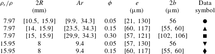
 $\unicode[STIX]{x1D6FF}=-h$) when the sphere is in contact with the pillars (figure 1b). The different spheres and micropillars used in the experiments of Chastel et al. (Reference Chastel, Gondret and Mongruel2016) (hereinafter referred to as CGM) are summarized in table 1 with the values of the density ratio
 $\unicode[STIX]{x1D70C}_{s}/\unicode[STIX]{x1D70C}$, the diameter
 $2R$, the Archimedes number
 $Ar$, the surface density
 $\unicode[STIX]{x1D719}$, the height and the width
 $2b$ of the square pillars. The aspect ratio of the pillars lies in the range
 $0.5\lesssim e/2b\lesssim 2.3$. The fluid is a silicon oil (Rhodorsil 47V1000) of density
 $\unicode[STIX]{x1D70C}=978~\text{kg}~\text{m}^{-3}$ and kinematic viscosity
 $\unicode[STIX]{x1D708}=\unicode[STIX]{x1D702}/\unicode[STIX]{x1D70C}=10^{-3}~\text{m}^{2}~\text{s}^{-1}$. The texture is completely wetted by the oil. The roughness
 $\unicode[STIX]{x1D709}$ of the sphere surface and the pillar surface is less than
 $0.1~\unicode[STIX]{x03BC}\text{m}$, thus negligibly small compared to the height
 $e$ and the width
 $2b$ of the pillars (
 $\unicode[STIX]{x1D709}\ll e,2b$). In addition, the geometrical sizes of the textures,
 $e$,
 $2b$ and
 $L$ are much smaller than the radius of the sphere (
 $e,2b,L\ll R$). The pillars, of density
 $\unicode[STIX]{x1D70C}_{w}=1300~\text{kg}~\text{m}^{3}$, have an elastic modulus
 $E=1.4$ GPa much less than that of the sphere, so the sphere may be considered as rigid. The range of the Archimedes number
 $Ar=\unicode[STIX]{x1D70C}(\unicode[STIX]{x1D70C}_{s}-\unicode[STIX]{x1D70C})gR^{3}/\unicode[STIX]{x1D702}^{2}$ is between 9.4 and 34.3. As
 $Ar=(9/4)Re_{St}$, where
 $Re_{St}=\unicode[STIX]{x1D70C}V_{St}(2R)/\unicode[STIX]{x1D702}$ is the Reynolds number based on the Stokes velocity,
 $V_{St}=2(\unicode[STIX]{x1D70C}_{s}-\unicode[STIX]{x1D70C})gR^{2}/(9\unicode[STIX]{x1D702})$, corresponding to the settling velocity of a sphere in an infinite fluid at low Reynolds number, the values of
 $Ar$ larger than
 $9/4$ in table 1 mean that fluid inertia plays a non-negligible role in these experiments. The sphere is initially maintained at rest by a magnet at the top wall of the cell located at the distance
 $H=40.8$ mm above the bottom wall, and released with a zero velocity. The release distance
 $h_{0}=H-2R$ for the sphere bottom thus varies in the range
 $24.9\leqslant h_{0}\leqslant 32.8~\text{mm}$ depending on the sphere size. With the interferometric technique of spatial resolution
 $0.2~\unicode[STIX]{x03BC}\text{m}$ and time resolution
 $2~\unicode[STIX]{x03BC}\text{s}$ used by CGM, the maximum sphere velocity that can be measured is
 $100~\text{mm}~\text{s}^{-1}$, which allows us to explore the sphere dynamics below or close above the bouncing transition, but not far above.
Parameters values for the different experimental sphere–microtexture configurations of Chastel et al. (Reference Chastel, Gondret and Mongruel2016), and data symbols used in figures 6(a), 8 and 10.

2.1 Typical experimental  $V(t)$, $h(t)$ and $V(h)$ curves


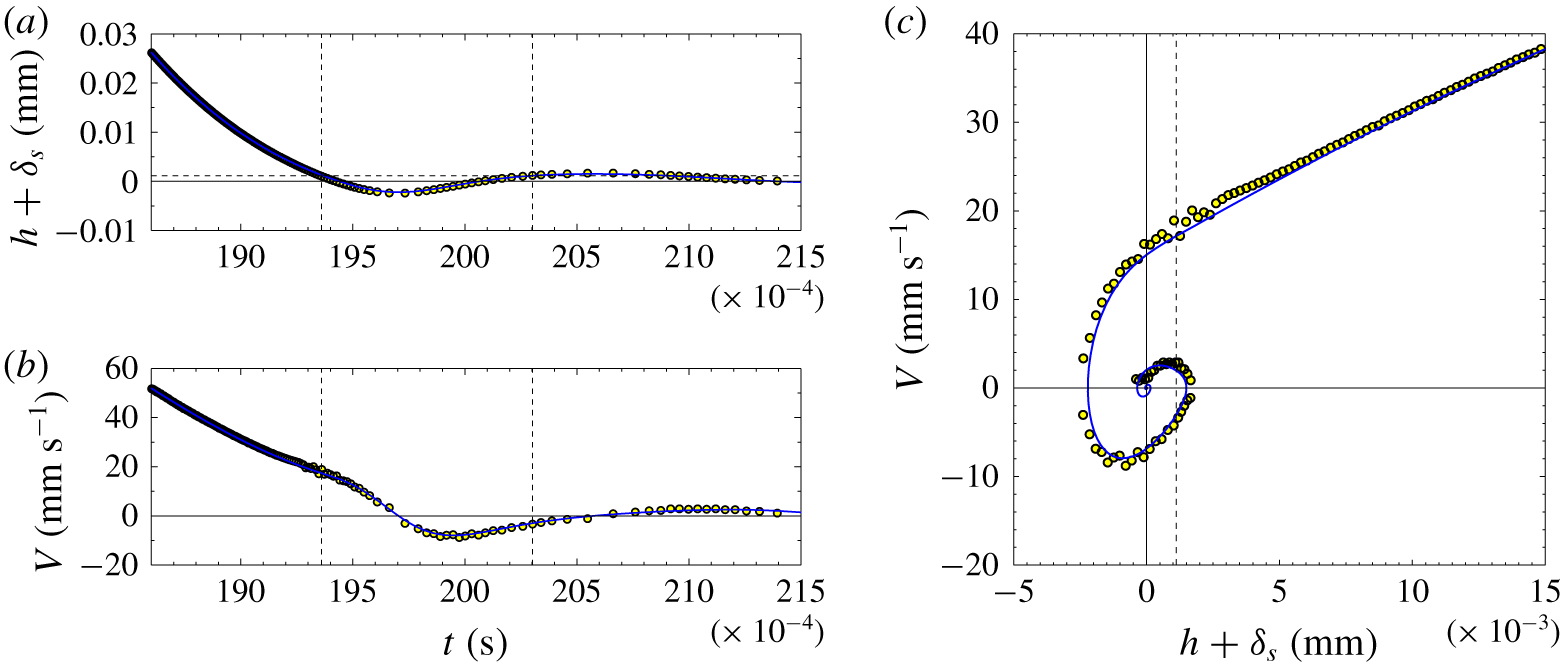
Figure 2 shows typical experimental curves obtained from the interferometric technique described in details in CGM. The instantaneous position  $h+\unicode[STIX]{x1D6FF}_{s}$ of the sphere, measured from the final rest position
 $-\unicode[STIX]{x1D6FF}_{s}$ on the deformed micropillars, and its instantaneous downward velocity
 $V=-\text{d}h/\text{d}t$ are plotted as a function of time in figures 2(a) and 2(b) for a steel sphere of density
 $\unicode[STIX]{x1D70C}_{s}=7800~\text{kg}~\text{m}^{-3}$ and diameter
 $2R=14~\text{mm}$ settling in silicon oil towards a microtextured wall with square pillars of surface fraction
 $\unicode[STIX]{x1D719}=0.15$, of height
 $e=60~\unicode[STIX]{x03BC}\text{m}$ and width
 $2b=57~\unicode[STIX]{x03BC}\text{m}$. In figure 2(c), the instantaneous velocity
 $V(t)$ is plotted as a function of its instantaneous position
 $h(t)+\unicode[STIX]{x1D6FF}_{s}$. When approaching the textured wall, the sphere velocity
 $V$ decreases from approximately
 $50~\text{mm}~\text{s}^{-1}$ at
 $25~\unicode[STIX]{x03BC}\text{m}$ from the wall, towards zero at a minimal and negative position corresponding to its maximal penetration distance into the pillars
 $\unicode[STIX]{x1D6FF}_{m}\simeq 3.5~\unicode[STIX]{x03BC}\text{m}$ before rebound. The final sphere position corresponds to its rest position on the deformed pillars with a static penetration distance of
 $\unicode[STIX]{x1D6FF}_{s}\simeq 1.1~\unicode[STIX]{x03BC}\text{m}$. In the case of figure 2, the sphere touches the top of the pillars at
 $h=0$ with an impact velocity
 $V_{i}\simeq 19~\text{mm}~\text{s}^{-1}$. The rebound velocity when the sphere just bounces back off the wall at
 $h=0$ is
 $V_{r}\simeq -4~\text{mm}~\text{s}^{-1}$, leading to the velocity ratio
 $-V_{r}/V_{i}\simeq 0.2$. The latter ratio defines the microscopic restitution coefficient of the solid collision taking into account only the dissipation during the sphere–pillar contact. The contact time (corresponding to
 $h\leqslant 0$) is
 $\unicode[STIX]{x1D70F}\simeq 0.95~\text{ms}$. Note that the sphere bouncing off the wall leads here to a tiny rebound of less than
 $1~\unicode[STIX]{x03BC}\text{m}$, which means that the present case is very close to the bouncing transition.
(a) Position  $h+\unicode[STIX]{x1D6FF}_{s}$ of the sphere to the wall relative to its final position
 $-\unicode[STIX]{x1D6FF}_{s}$ and (b) velocity
 $V$ as a function of time
 $t$ for a steel sphere of diameter
 $2R=14~\text{mm}$ settling in 47V1000 silicon oil toward a horizontal textured wall with square pillars of surface fraction
 $\unicode[STIX]{x1D719}=0.15$, height
 $e=60~\unicode[STIX]{x03BC}\text{m}$ and width
 $2b=57~\unicode[STIX]{x03BC}\text{m}$, impacting it at the Stokes number
 $St_{i}=0.25$. (c) Instantaneous velocity
 $V$ of the sphere as a function of its instantaneous position
 $h+\unicode[STIX]{x1D6FF}_{s}$. The (a) horizontal and (c) vertical red dotted lines indicate the position of the top of the underformed textures (
 $h=0$) with
 $\unicode[STIX]{x1D6FF}_{s}=1.1~\unicode[STIX]{x03BC}\text{m}$. The two vertical dotted lines in (a,b) indicate the times of initial and final solid contact corresponding to the time duration
 $\unicode[STIX]{x1D70F}=9.6~\text{ms}$. The solid curves correspond to model equations (2.1) and (2.3) with
 $\unicode[STIX]{x1D6FC}=0.9$ and
 $s=35~\unicode[STIX]{x03BC}\text{m}$.

2.2 Modelling the sphere motion during the approach phase
When the sphere is near but not touching the wall ( $h>0$), the forces acting on it are the constant driving gravity force
 $F_{g}=(4/3)\unicode[STIX]{x03C0}R^{3}\unicode[STIX]{x1D70C}_{s}g$ and the fluid forces, which can be decomposed into three parts: (i) the static part corresponding to the constant Archimedean buoyancy force
 $F_{A}=-(4/3)\unicode[STIX]{x03C0}R^{3}\unicode[STIX]{x1D70C}g$ from the static pressure field; (ii) the (quasi-)steady part of the drag force
 $F_{D}(t)=-C_{Dw}6\unicode[STIX]{x03C0}\unicode[STIX]{x1D702}RV(t)$; and (iii) the unsteady part of the drag force corresponding to the added-mass term
 $F_{am}(t)=-C_{am}(4/3)\unicode[STIX]{x03C0}R^{3}\unicode[STIX]{x1D70C}\text{d}V/\text{d}t$. The two last fluid force terms are modified by the near wall as follows.
Concerning the coefficient of the added-mass term, its value  $C_{am}=1/2$ from potential flow theory for an isolated sphere far from any boundary is increased by the near wall. The modified value for a sphere in normal motion relative to a flat wall can be calculated from potential flow theory using images and is given as a series with
 $C_{am}=1/2+3R/16(R+h)$ at first order (Milne-Thomson Reference Milne-Thomson1968) and with the approximate expression
 $C_{am}\simeq 1/2+0.8(1.9+h/R)^{-3.9}$ proposed by Ardekani & Rangel (Reference Ardekani and Rangel2008) for all
 $h/R$. In the present case where the sphere is very close to the wall with vanishing
 $h/R$ values, this coefficient can be considered as constant with the value
 $C_{am}\simeq 0.56$, only 12 % larger than the usual far value 0.5.
The (quasi-)steady drag force term is also increased by the near wall. For a smooth sphere at vanishing  $Re$ number in normal motion close to a smooth solid wall (
 $h/R\ll 1$), the huge wall-correction factor to the Stokes force
 $F_{St}=-6\unicode[STIX]{x03C0}R\unicode[STIX]{x1D702}V$ is
 $C_{Dw}=R/h$, leading to the well known lubrication drag force
 $F_{D}=-6\unicode[STIX]{x03C0}R^{2}\unicode[STIX]{x1D702}V/h$, that diverges at vanishing
 $h$ for smooth surfaces. Here, due to the wall textures, the lubrication force is regularized during the whole dynamics by a characteristic length
 $s$, and is
 $F_{D}=-6\unicode[STIX]{x03C0}R^{2}\unicode[STIX]{x1D702}V/(h+s)$. Hence, the drag on the sphere at the distance
 $h$ from the top of the micropillars is the same as near an imaginary smooth wall that would be located at a slightly larger distance
 $h+s$. The characteristic length
 $s$ is the near-field (valid for
 $h\ll L$) shift length introduced by Chastel & Mongruel (Reference Chastel and Mongruel2019), which depends on the geometrical parameters of the pillar array (
 $e$,
 $L$ and
 $2b$ or
 $\unicode[STIX]{x1D719}$), as reported and discussed in details in appendix A. A semiempirical correlation based on theoretical arguments developed in Seiwert, Clanet & Quéré (Reference Seiwert, Clanet and Quéré2011) and Chastel & Mongruel (Reference Chastel and Mongruel2016) gives
 $s\simeq e(1-\unicode[STIX]{x1D719})[1+\unicode[STIX]{x1D6FD}(\unicode[STIX]{x1D719})(e/L)^{2}]^{-1/3}$, where the coefficient
 $\unicode[STIX]{x1D6FD}$, which can be estimated from the work of Kuwabara (Reference Kuwabara1959), varies from 14 to 90 for
 $\unicode[STIX]{x1D719}$ varying from 0.05 to 0.30. This shift length
 $s$, which can be seen as an effective hydrodynamic roughness, varies between 17 and
 $71~\unicode[STIX]{x03BC}\text{m}$ in the experiments considered here. It is thus much smaller than the size of the sphere but much larger than its surface roughness.
In the case of finite Reynolds number, Mongruel et al. (Reference Mongruel, Lamriben, Yahiaoui and Feuillebois2010) have observed that the sphere velocity varies linearly with the distance  $h$ as
 $V=V_{0}h/R$ in the last regime before contact, but with a typical velocity
 $V_{0}$ slightly larger from
 $V_{St}$. Hence, an additional numerical prefactor
 $\unicode[STIX]{x1D6FC}=V_{St}/V_{0}$ slightly smaller than unity is needed to fit the experimental data. The coefficient
 $\unicode[STIX]{x1D6FC}$ measured for spheres approaching a smooth surface varies typically between 0.95 and 0.85 with an average value 0.9 for the experiments considered here. This prefactor may reflect some complex unsteady effect such as the integral history force.
The sphere motion can thus be modelled by the equation
 $$\begin{eqnarray}\frac{4}{3}\unicode[STIX]{x03C0}R^{3}(\unicode[STIX]{x1D70C}_{s}+C_{am}\unicode[STIX]{x1D70C})\frac{\text{d}V}{\text{d}t}=\frac{4}{3}\unicode[STIX]{x03C0}R^{3}(\unicode[STIX]{x1D70C}_{s}-\unicode[STIX]{x1D70C})g-\frac{6\unicode[STIX]{x03C0}R^{2}\unicode[STIX]{x1D702}\unicode[STIX]{x1D6FC}V}{h+s}.\end{eqnarray}$$
This equation can be written in a dimensionless form with the sphere radius  $R$ for the length scale, the impact velocity
 $V_{i}$ for the velocity scale and the ratio
 $R/V_{i}$ for the time scale
 $$\begin{eqnarray}\frac{2}{9}\frac{(\unicode[STIX]{x1D70C}_{s}+C_{am}\unicode[STIX]{x1D70C})RV_{i}}{\unicode[STIX]{x1D702}}\frac{\text{d}\tilde{V}}{\text{d}\tilde{t}}=\frac{V_{St}}{V_{i}}-\frac{\unicode[STIX]{x1D6FC}\tilde{V}}{\tilde{h}+\tilde{s}},\end{eqnarray}$$
where  $\tilde{V}=V/V_{i}$,
 $\tilde{h}=h/R$,
 $\tilde{s}=s/R$ and
 $\tilde{t}=tV_{i}/R$. Two dimensionless numbers appear in this dimensionless equation: the impact Stokes number
 $St_{i}=2(\unicode[STIX]{x1D70C}_{s}+C_{am}\unicode[STIX]{x1D70C})RV_{i}/9\unicode[STIX]{x1D702}$ based on the impact velocity and taking into account the added mass effect as introduced by Legendre et al. (Reference Legendre, Zenit, Daniel and Guiraud2006); and the velocity ratio
 $V_{St}/V_{i}=4Ar/9Re_{i}$, where
 $Re_{i}=\unicode[STIX]{x1D70C}V_{i}(2R)/\unicode[STIX]{x1D702}$ is the Reynolds number based on the impact velocity
 $V_{i}$. Following Izard et al. (Reference Izard, Bonometti and Lacaze2014), the three dimensionless numbers that govern the approach dynamics of the sphere towards the microtextured wall numbers can be either the a priori known
 $Ar$ and density ratio
 $\unicode[STIX]{x1D70C}_{s}/\unicode[STIX]{x1D70C}$ or the a posteriori measured
 $St_{i}$ and
 $Re_{i}$, together with the dimensionless shift length
 $s/R$ that characterizes here the hydrodynamic effect of the micropillars. The consequences of the shift length
 $s$ are a finite pressure and drag force, and a non-zero velocity for the sphere at
 $h=0$. An estimation of elastic deformation of the wall textures detailed in appendix B gives very small deformation, typically between 0.001 and
 $0.1~\unicode[STIX]{x03BC}\text{m}$, which is smaller or of the order of the microscopic roughness of the sphere surface and texture surface. In the present modelling, we thus do not consider any pillar deformation when
 $h>0$ and consider that solid contact occurs at
 $h=0$.
2.3 Modelling the sphere motion during the contact phase
When  $h\leqslant 0$, the sphere is thus considered to be in solid contact with the textured wall. For a wall covered by an array of micropillars, CGM has derived a contact model by considering that the pillars behave as independent springs. The nonlinear contact force is
 $F_{w}=-\unicode[STIX]{x03C0}\unicode[STIX]{x1D719}ER\unicode[STIX]{x1D6FF}^{2}/e$, where
 $\unicode[STIX]{x1D6FF}=-h$ corresponds now to the wall deformation, with a power exponent 2 for
 $\unicode[STIX]{x1D6FF}$, which is different from the exponent 3/2 for the classical Hertz force valid for a sphere in contact with a smooth elastic half-plane. This contact force, validated experimentally by CGM and then by Maruoka (Reference Maruoka2019), has been derived under different assumptions: (i) an elastic response of the pillars; (ii) a quasi-static deformation; and (iii) a contact area embedding several pillars. In the set of experiments considered here, these assumptions are satisfied: (i) the relative deformation
 $\unicode[STIX]{x1D6FF}_{m}/e$ of the pillars remains smaller than
 $10^{-1}$, thus in the elastic regime. (ii) The solid collision time
 $\unicode[STIX]{x1D70F}\simeq 1$ ms remains much larger than the propagation time of the deformation in the pillars
 $e/c\simeq 0.1~\unicode[STIX]{x03BC}\text{s}$ where
 $c=(E/\unicode[STIX]{x1D70C}_{w})^{1/2}\simeq 10^{3}$ m/s is the sound velocity in the pillars. Following the criterion
 $(V_{i}/c)^{3/5}\ll 1$ expressed by Hunter (Reference Hunter1957) in terms of a velocity ratio rather than of a time ratio for the Hertz collision of a sphere onto a smooth wall, the present quasi-static criterion, which is satisfied for the present sphere collision onto the textured wall, can be expressed as
 $(V_{i}\unicode[STIX]{x1D719}\unicode[STIX]{x1D70C}_{w}e^{2}/c\unicode[STIX]{x1D70C}_{s}R^{2})^{1/3}\ll 1$. (iii) The number of pillars embedded in the solid collision within the contact disk area of radius
 $(2R\unicode[STIX]{x1D6FF}_{m})^{1/2}$, and which can be thus estimated as
 $N\simeq 2\unicode[STIX]{x03C0}R\unicode[STIX]{x1D6FF}_{m}/L^{2}$, is in the range
 $3\lesssim N\lesssim 37$. The contact force derived by CGM is a generalization of the elastic foundation model of Johnson (Reference Johnson1985) for solid fraction
 $\unicode[STIX]{x1D719}\neq 1$, but it would not be valid at the opposite limit of vanishing
 $\unicode[STIX]{x1D719}$ where only one pillar would be embedded in the contact (Ledesma-Alonso et al. Reference Ledesma-Alonso, Raphaël, Léger, Restagno and Poulard2016). Assuming that the added-mass force and the drag force discussed in § 2.2 remain unchanged during contact, the sphere motion can thus be modelled by the equation
 $$\begin{eqnarray}\frac{4}{3}\unicode[STIX]{x03C0}R^{3}(\unicode[STIX]{x1D70C}_{s}+C_{am}\unicode[STIX]{x1D70C})\frac{\text{d}V}{\text{d}t}=\frac{4}{3}\unicode[STIX]{x03C0}R^{3}(\unicode[STIX]{x1D70C}_{s}-\unicode[STIX]{x1D70C})g-\frac{6\unicode[STIX]{x03C0}R^{2}\unicode[STIX]{x1D702}\unicode[STIX]{x1D6FC}V}{s-\unicode[STIX]{x1D6FF}}-\frac{\unicode[STIX]{x03C0}\unicode[STIX]{x1D719}ER\unicode[STIX]{x1D6FF}^{2}}{e}.\end{eqnarray}$$
This equation governs the sphere motion when  $h\leqslant 0$ during the contact with the pillars until the solid contact breaks with a non-zero rebound velocity
 $-V_{r}$ at
 $h=0$, or until the sphere stops (with
 $V=0$ and
 $\text{d}V/\text{d}t=0$) at its final resting position
 $\unicode[STIX]{x1D6FF}_{s}/R=[4e(\unicode[STIX]{x1D70C}_{s}-\unicode[STIX]{x1D70C})g/3\unicode[STIX]{x1D719}E]^{1/2}$, resulting from the balance of apparent weight and elastic contact force. The corresponding dimensionless equation is
 $$\begin{eqnarray}St_{i}\frac{\text{d}\tilde{V}}{\text{d}\tilde{t}}=\frac{4Ar}{9Re_{i}}-\frac{\unicode[STIX]{x1D6FC}\tilde{V}}{\tilde{s}-\tilde{\unicode[STIX]{x1D6FF}}}-\frac{\unicode[STIX]{x1D719}ER^{2}}{6e\unicode[STIX]{x1D702}V_{i}}\tilde{\unicode[STIX]{x1D6FF}}^{2},\end{eqnarray}$$
where  $\tilde{\unicode[STIX]{x1D6FF}}=\unicode[STIX]{x1D6FF}/R$. Three main dimensionless numbers appear in this dimensionless equation: the impact Stokes number
 $St_{i}$; a gravitoviscous number corresponding here to the velocity ratio
 $V_{St}/V_{i}=4Ar/9Re_{i}$; and an elastoviscous parameter
 $\unicode[STIX]{x1D719}ER^{2}/6e\unicode[STIX]{x1D702}V_{i}$. The latter parameter corresponds to the inverse of the elastic parameter introduced by Davis et al. (Reference Davis, Serayssol and Hinch1986) for the collision of an elastic sphere onto a smooth wall, but is somewhat different here due to the micropillars. Note that this elastic parameter is very large as the dimensionless deformation
 $\tilde{\unicode[STIX]{x1D6FF}}$ remains very small.
2.4 Comparison between the model and experiments
Let us now compare the data with the modelling. The curves obtained by numerical integration of the model equations (2.1) and (2.3) are very close to the data points of figure 2 all along the sphere motion, not only in the approach phase before the wall impact, but also during the contact and the subsequent bouncing. In particular, the penetration distance  $\unicode[STIX]{x1D6FF}_{m}$ and the bouncing height are remarkably well predicted. The dimensionless number values for this case are
 $St_{i}\simeq 0.25$,
 $V_{St}/V_{i}=4Ar/9Re_{i}\simeq 39$ and
 $\unicode[STIX]{x1D719}ER^{2}/6e\unicode[STIX]{x1D702}V_{i}\simeq 1.54\times 10^{9}$. Note that the two corrections for the drag force used here are not fitting parameters, but the near-field shift length
 $s\simeq 35~\unicode[STIX]{x03BC}\text{m}$ (
 $\tilde{s}\simeq 5\times 10^{-3}$) and the factor
 $\unicode[STIX]{x1D6FC}\simeq 0.9$, obtained from previous experiments at small Reynolds number near the same micropillars (Chastel & Mongruel Reference Chastel and Mongruel2019) and at finite Reynolds number near a smooth wall (Mongruel et al. Reference Mongruel, Lamriben, Yahiaoui and Feuillebois2010), respectively. This shift length, which is smaller than, but of the order of, the pillar height (
 $s/e\simeq 0.58$), corresponds to the effective hydrodynamic roughness of the wall. Taking into account the drag force when the sphere is in solid contact with the wall is crucial for modelling correctly the bouncing dynamics: ignoring the drag force would indeed lead to a significant overestimation of the pillar deformation (4.4 instead of
 $3.5~\unicode[STIX]{x03BC}\text{m}$), and then a large overestimation of the subsequent rebound velocity (
 $-17$ instead of
 $-4~\text{mm}~\text{s}^{-1}$) and of the bouncing height in the fluid (5 instead of
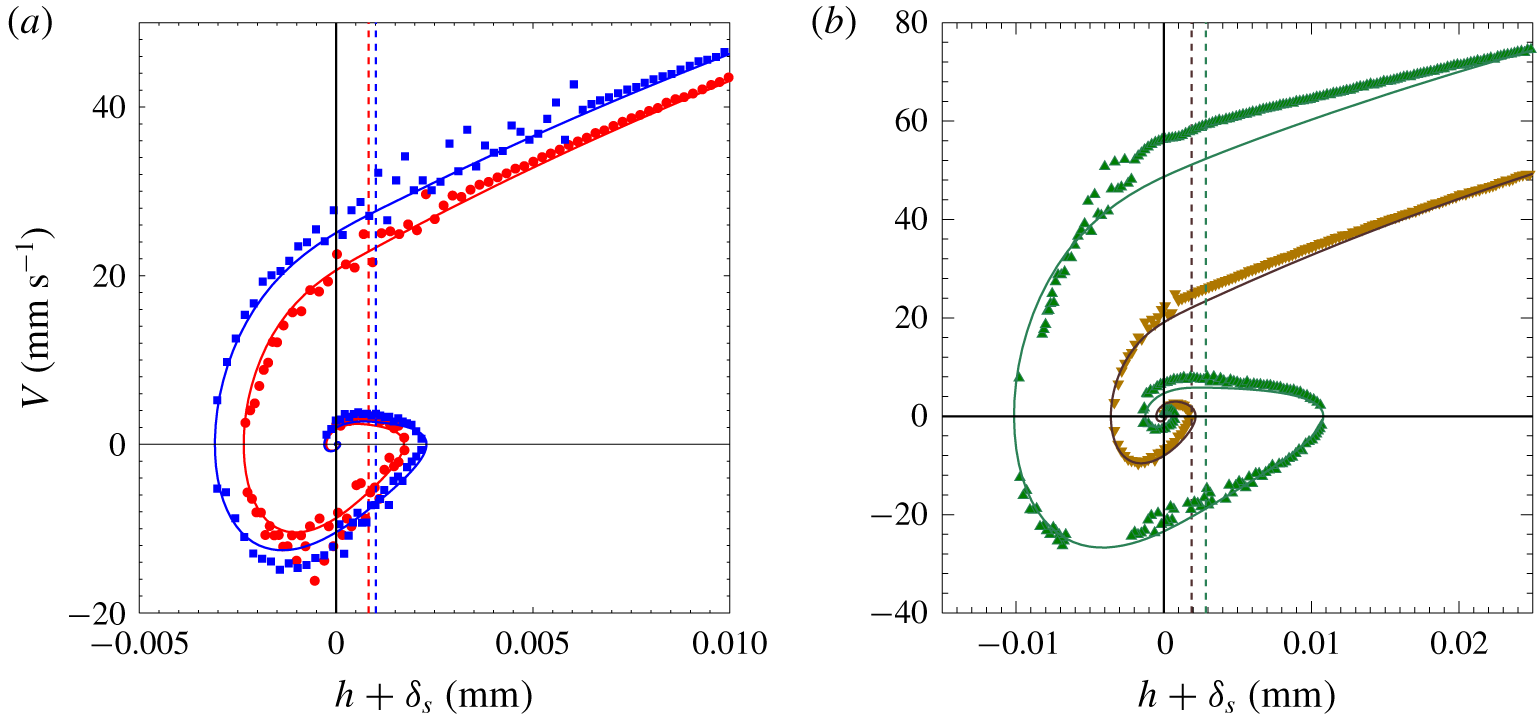
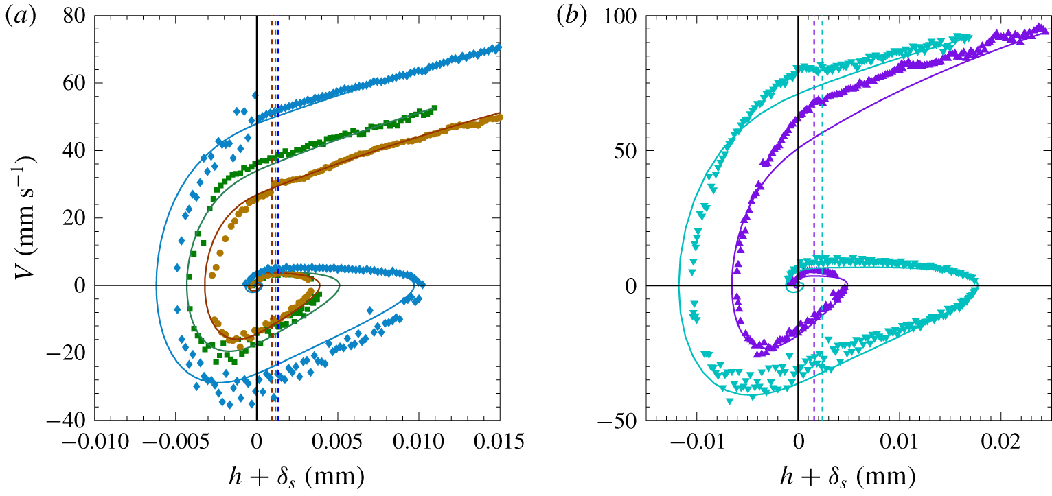
 $0.5~\unicode[STIX]{x03BC}\text{m}$). The very good agreement that is observed between modelling and experimental data when taking into account all the terms in (2.1) and (2.3) is also observed for many other cases, examples of which are depicted in figure 3 and figure 4 for the bouncing motion of a steel sphere and a tungsten carbide sphere, respectively, on pillar arrays of various geometries.
Figure 3(a) shows two typical  $V(h)$ curves for a steel sphere of diameter
 $2R=15~\text{mm}$ colliding with micropillars of the same surface fraction
 $\unicode[STIX]{x1D719}=0.30$ and of two different heights (
 $e=57$ and
 $85~\unicode[STIX]{x03BC}\text{m}$) with approximately the same width (
 $2b\simeq 100~\unicode[STIX]{x03BC}\text{m}$). As expected, the impact velocity is slightly larger for higher pillars:
 $V_{i}\simeq 27~\text{mm}~\text{s}^{-1}$ corresponding to an impact Stokes number
 $St_{i}\simeq 0.39$ for
 $e=85~\unicode[STIX]{x03BC}\text{m}$ when compared to
 $V_{i}\simeq 23~\text{mm}~\text{s}^{-1}$ (
 $St_{i}\simeq 0.33$) for
 $e=57~\unicode[STIX]{x03BC}\text{m}$. The modelling uses a correction factor
 $\unicode[STIX]{x1D6FC}\simeq 0.9$, and shift lengths
 $s=26.5~\unicode[STIX]{x03BC}\text{m}$ and
 $s=24.5~\unicode[STIX]{x03BC}\text{m}$, respectively, for the higher and lowest pillars. In the two cases, very small rebounds of approximately 2 and
 $3~\unicode[STIX]{x03BC}\text{m}$ are observed.
Instantaneous velocity  $V$ as a function of the instantaneous position
 $h+\unicode[STIX]{x1D6FF}_{s}$ relative to its final static position
 $-\unicode[STIX]{x1D6FF}_{s}$ for a steel sphere of diameter (a)
 $2R=15~\text{mm}$ impacting a textured wall with micropillars of surface fraction
 $\unicode[STIX]{x1D719}=0.30$, height
 $e=57~\unicode[STIX]{x03BC}\text{m}$ and width
 $2b=102~\unicode[STIX]{x03BC}\text{m}$ (●) or
 $e=85~\unicode[STIX]{x03BC}\text{m}$ and
 $2b=106~\unicode[STIX]{x03BC}\text{m}$ (▪); and for (b)
 $2R=14~\text{mm}$,
 $\unicode[STIX]{x1D719}=0.05$,
 $2b=56~\unicode[STIX]{x03BC}\text{m}$ and
 $e=57~\unicode[STIX]{x03BC}\text{m}$ (▿) or
 $e=130~\unicode[STIX]{x03BC}\text{m}$ (▵). Model equations (2.1) and (2.3) with
 $\unicode[STIX]{x1D6FC}=0.9$ and with (a)
 $s=24.5~\unicode[STIX]{x03BC}\text{m}$ (——, red) or
 $s=26.5~\unicode[STIX]{x03BC}\text{m}$ (——, blue); and (b)
 $s=43~\unicode[STIX]{x03BC}\text{m}$ (——, brown) or
 $s=57~\unicode[STIX]{x03BC}\text{m}$ (——, green).

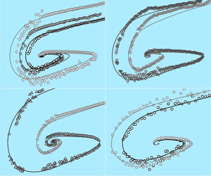
Same as figure 3 for a tungsten carbide sphere ( $2R=8~\text{mm}$) towards a textured wall with pillars of (a) surface fraction
 $\unicode[STIX]{x1D719}=0.15$ and of height
 $e=60~\unicode[STIX]{x03BC}\text{m}$ and width
 $2b=57~\unicode[STIX]{x03BC}\text{m}$ (●),
 $e=91~\unicode[STIX]{x03BC}\text{m}$ and
 $2b=60~\unicode[STIX]{x03BC}\text{m}$ (▪), or
 $e=117~\unicode[STIX]{x03BC}\text{m}$ and
 $2b=55~\unicode[STIX]{x03BC}\text{m}$ (♢); (b)
 $\unicode[STIX]{x1D719}=0.05$,
 $2b=56~\unicode[STIX]{x03BC}\text{m}$ and
 $e=57~\unicode[STIX]{x03BC}\text{m}$ (▴) or
 $e=130~\unicode[STIX]{x03BC}\text{m}$ (▾). The two vertical dotted lines stand for the top of the undeformed textures at
 $h=0$ in each case. The solid curves corresponds to model equations (2.1) and (2.3) with
 $\unicode[STIX]{x1D6FC}=0.85$ and with (a)
 $s=35~\unicode[STIX]{x03BC}\text{m}$ (——, brown),
 $s=39~\unicode[STIX]{x03BC}\text{m}$ (——, green) or
 $s=42~\unicode[STIX]{x03BC}\text{m}$ (——, blue); and (b)
 $s=27~\unicode[STIX]{x03BC}\text{m}$ (——, purple) or
 $s=47~\unicode[STIX]{x03BC}\text{m}$ (——, blue).

Two other typical  $V(h)$ curves are shown in figure 3(b) for a steel sphere of diameter
 $2R=14~\text{mm}$ colliding with a wall with micropillars of smaller surface fraction (
 $\unicode[STIX]{x1D719}=0.05$) and of two different heights (
 $e=57$ and
 $130~\unicode[STIX]{x03BC}\text{m}$) with the same width (
 $2b\simeq 56~\unicode[STIX]{x03BC}\text{m}$). Compared to figure 3(a), the effect of decreasing the pillar surface fraction and increasing the pillar height is seen to amplify the rebound, leading to a larger impact velocity
 $V_{i}\simeq 59~\text{mm}~\text{s}^{-1}$ (
 $St_{i}\simeq 0.79$) for
 $e=130~\unicode[STIX]{x03BC}\text{m}$. As expected, the static deformation is larger for the higher pillars as the contact force is weaker:
 $\unicode[STIX]{x1D6FF}_{s}\simeq 3$ for
 $e=130~\unicode[STIX]{x03BC}\text{m}$ compared to
 $2~\unicode[STIX]{x03BC}\text{m}$ for
 $e=57~\unicode[STIX]{x03BC}\text{m}$. Interestingly, the case
 $e=57~\unicode[STIX]{x03BC}\text{m}$ for which
 $V_{i}\simeq 25~\text{mm}~\text{s}^{-1}$ (
 $St_{i}\simeq 0.33$) corresponds exactly to the bouncing transition as the maximal position of the sphere after the collision is here
 $h=0$, i.e. the sphere remains in contact with the pillars. The case at
 $St_{i}\simeq 0.79$ is clearly above the bouncing transition with a bouncing height of
 $7~\unicode[STIX]{x03BC}\text{m}$. Using the correction factor
 $\unicode[STIX]{x1D6FC}\simeq 0.9$ together with the shift length
 $s=57~\unicode[STIX]{x03BC}\text{m}$ and
 $s=43~\unicode[STIX]{x03BC}\text{m}$ for the highest and the lowest pillars, respectively, it can be seen that the modelling does not fit perfectly the approach phase in the case
 $e=130~\unicode[STIX]{x03BC}\text{m}$, but performs very well in the contact and rebound phases.
Finally, figures 4(a) and 4(b) show various  $V(h)$ curves for a tungsten carbide sphere of diameter
 $2R=8~\text{mm}$ approaching a wall with micropillars of surface fraction
 $\unicode[STIX]{x1D719}=0.15$ and
 $\unicode[STIX]{x1D719}=0.05$, respectively, and of different heights
 $e$ (ranging from 60 to
 $130~\unicode[STIX]{x03BC}\text{m}$) with approximately the same width
 $2b$. Again, we observe that for a given pillar surface fraction, increasing the pillar height amplifies the bouncing, with higher impact velocities and hence larger penetration depths and also larger bouncing heights. For instance, at
 $\unicode[STIX]{x1D719}=0.15$,
 $V_{i}\simeq 38~\text{mm}~\text{s}^{-1}$ (
 $St_{i}\simeq 0.56$) for
 $e=91~\unicode[STIX]{x03BC}\text{m}$ compared to
 $V_{i}\simeq 51~\text{mm}~\text{s}^{-1}$ (
 $St_{i}\simeq 0.76$) for
 $e=117~\unicode[STIX]{x03BC}\text{m}$. The same observation can be made when decreasing the pillar surface fraction at a given pillar height: for
 $e=57~\unicode[STIX]{x03BC}\text{m}$,
 $V_{i}\simeq 30~\text{mm}~\text{s}^{-1}$ (
 $St_{i}\simeq 0.44$) at
 $\unicode[STIX]{x1D719}=0.15$ compared to
 $V_{i}\simeq 68~\text{mm}~\text{s}^{-1}$ (
 $St_{i}\simeq 1$) at
 $\unicode[STIX]{x1D719}=0.05$. The modelling still gives correct results, but it happens to overestimate the bouncing height or the penetration distance in some cases.
All the results presented in figures 2, 3 and 4 concern cases where small bouncing of the spheres off the wall is observed thus slightly above the bouncing transition. In some cases, no bouncing of the spheres off the wall is observed as shown in figure 5. In that figure, the experimental measurements of the sphere motion are plotted for four different diameters of steel sphere impacting the same textured wall at a finite but very low velocity. Indeed the impact velocity taken at the top of the underformed structure ( $h=0$) is
 $V_{i}\approx 1.4,1.8,2.2$ and
 $2.8~\text{mm}~\text{s}^{-1}$, corresponding to very low impact Stokes number,
 $0.014\lesssim St_{i}\lesssim 0.04$. The model indeed predicts the ‘sticking’ collision observed experimentally: the spheres come to rest with a strong monotonic decrease of velocity down to their final position
 $h=-\unicode[STIX]{x1D6FF}_{s}$.
3 The critical Stokes number for bouncing
The fact that a sphere approaching a wall will rebound or not off the wall, is here related to viscous dissipation. This viscous dissipation arises during the two phases of the sphere motion: (i) the approach towards the textured wall and (ii) the solid contact with the micropillars during the collision.
Let us first consider the approach phase. As seen in figure 11, the apparent weight can be neglected when compared to the large lubrication force near the wall and the sphere is thus strongly decelerated. The balance of sphere inertia (with the added-mass term) and lubrication drag in equation (2.1) yields a logarithmic variation of the velocity  $V(h)$ of the sphere as a function of the distance
 $h>0$ (Davis et al. Reference Davis, Serayssol and Hinch1986). With the impact velocity
 $V_{i}$ taken as the reference velocity at
 $h=0$, one obtains
 $$\begin{eqnarray}\frac{V(h)}{V_{i}}\simeq 1+\frac{\unicode[STIX]{x1D6FC}}{St_{i}}\ln \left(\frac{h+s}{s}\right).\end{eqnarray}$$
To obtain an estimate of the velocity  $V_{\infty }$ far from the wall, we extrapolate (3.1) up to the distance
 $h=R$, at which the lubrication drag force due to the wall becomes of the order of the Stokes drag force in an infinite fluid (
 $C_{w}\simeq 1$). As
 $R\gg s$ in our case, the estimate
 $V_{\infty }=V(h=R)$ of the velocity
 $V_{\infty }$ far from the wall is thus given by
 $$\begin{eqnarray}\frac{V_{\infty }}{V_{i}}\simeq 1+\frac{\unicode[STIX]{x1D6FC}}{St_{i}}\ln \left(\frac{R}{s}\right).\end{eqnarray}$$
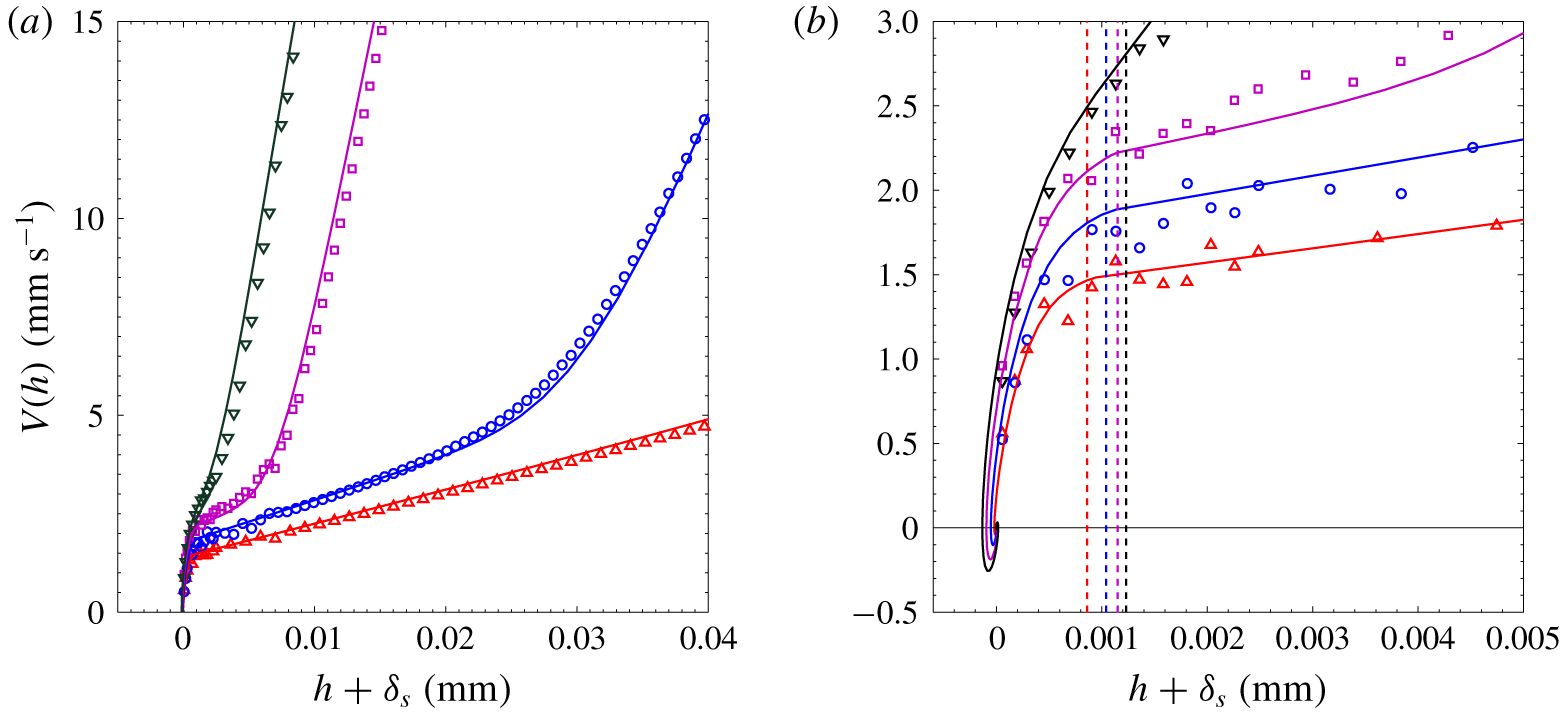
(a) Same as figure 3 for steel spheres of diameter  $2R=10.5$ (▵), 12.7 (○), 14 (▫) and 15 mm (▿), towards a textured wall with pillars of surface fraction
 $\unicode[STIX]{x1D719}=0.05$ and of height
 $e=21~\unicode[STIX]{x03BC}\text{m}$ and width
 $2b=57~\unicode[STIX]{x03BC}\text{m}$. The solid curves corresponds to model equations (2.1) and (2.3) with
 $s=17~\unicode[STIX]{x03BC}\text{m}$ and (a)
 $\unicode[STIX]{x1D6FC}=0.98$ (——, red), 0.95 (——, blue), 0.90 (——, purple), 0.90 (——). (b) Zoom on panel (a) with vertical dotted lines standing for the top of the undeformed textures at
 $h=0$ with
 $\unicode[STIX]{x1D6FF}_{s}=0.86$ (- - -, red), 1.04 (- - -, blue), 1.15 (- - -, purple) and
 $1.23~\unicode[STIX]{x03BC}\text{m}$ (- - -).

Another typical velocity of approach is provided by the terminal settling velocity  $V_{T}$ resulting from the balance of the effective weight of the sphere and the drag force far from the wall. In the present situation where fluid inertia is not negligible, the latter drag force is
 $-6\unicode[STIX]{x03C0}\unicode[STIX]{x1D702}RV(1+3Re/16)$, i.e. the Stokes drag modified by the Oseen correction for small fluid inertia (
 $Re$ is here the Reynolds number based on the velocity
 $V$ of the sphere). The terminal velocity
 $V_{T}$ is thus smaller than the Stokes velocity
 $V_{St}$. In the case of figure 2, the terminal settling velocity is
 $V_{T}=376~\text{mm}~\text{s}^{-1}$, whereas the estimate velocity far from the wall is
 $V_{\infty }=378~\text{mm}~\text{s}^{-1}$, from equation (3.2) with
 $V_{i}\simeq 19~\text{mm}~\text{s}^{-1}$ (
 $St_{i}\simeq 0.25$),
 $R=7~\text{mm}$,
 $s\simeq 35~\unicode[STIX]{x03BC}\text{m}$ and
 $\unicode[STIX]{x1D6FC}\simeq 0.9$. In that case, the two velocities
 $V_{\infty }$ and
 $V_{T}$ are very close to each other. In most cases,
 $V_{\infty }$ is slightly smaller than
 $V_{T}$, in the range
 $0.8V_{T}\lesssim V_{\infty }\lesssim V_{T}$, as the experimental cell is not high enough for the sphere starting from rest at the top of the cell to reach its terminal velocity. We thus choose here to use the characteristic approach velocity
 $V_{\infty }$ at the distance
 $R$ from the wall, to infer a macroscopic Stokes number
 $St$ from the experimental conditions
 $$\begin{eqnarray}St=St_{i}\frac{V_{\infty }}{V_{i}}\simeq St_{i}+\unicode[STIX]{x1D6FC}\ln \left(\frac{R}{s}\right).\end{eqnarray}$$
This Stokes number  $St=2(\unicode[STIX]{x1D70C}_{s}+C_{am}\unicode[STIX]{x1D70C})RV_{\infty }/9\unicode[STIX]{x1D702}$ is close to the one based on the terminal velocity
 $V_{T}$ (Legendre et al. Reference Legendre, Zenit, Daniel and Guiraud2006; Ardekani & Rangel Reference Ardekani and Rangel2008; Izard et al. Reference Izard, Bonometti and Lacaze2014). In the case of figure 2, this global Stokes number is
 $St\simeq 4.5$, much larger than the impact Stokes number
 $St_{i}\simeq 0.25$.
Let us now estimate the fluid dissipation during the sphere collision with the pillars. During this collision, the contact force on the sphere comes into play and the sphere motion is now given by (2.3). Neglecting the gravity force, the corresponding equation for the energy is given by
 $$\begin{eqnarray}\frac{2}{3}\unicode[STIX]{x03C0}R^{3}(\unicode[STIX]{x1D70C}_{s}+C_{am}\unicode[STIX]{x1D70C})V_{i}^{2}=\frac{2}{3}\unicode[STIX]{x03C0}R^{3}(\unicode[STIX]{x1D70C}_{s}+C_{am}\unicode[STIX]{x1D70C})V(t)^{2}+\frac{\unicode[STIX]{x03C0}}{3}\unicode[STIX]{x1D719}E_{w}\frac{R}{e}\unicode[STIX]{x1D6FF}(t)^{3}-\int _{0}^{\unicode[STIX]{x1D6FF}}\frac{6\unicode[STIX]{x03C0}R^{2}\unicode[STIX]{x1D702}\unicode[STIX]{x1D6FC}V(t)}{s-\unicode[STIX]{x1D6FF}}\,\text{d}\unicode[STIX]{x1D6FF}.\end{eqnarray}$$
In this equation, the initial kinetic energy  $E_{ki}=(1/2)M_{eff}V_{i}^{2}$ of the sphere of effective mass
 $M_{eff}=(4/3)\unicode[STIX]{x03C0}R^{3}(\unicode[STIX]{x1D70C}_{s}+C_{am}\unicode[STIX]{x1D70C})$ corresponding to its own mass and the fluid added-mass is partly transferred to the pillars from elastic deformation with the potential energy term
 $E_{p}=\int _{0}^{\unicode[STIX]{x1D6FF}}F_{w}\,\text{d}\unicode[STIX]{x1D6FF}$ and is partly lost in the fluid flow from viscous dissipation with the term
 $E_{d}=\int _{0}^{\unicode[STIX]{x1D6FF}}F_{D}\,\text{d}\unicode[STIX]{x1D6FF}$. For a zero fluid dissipation (
 $\unicode[STIX]{x1D702}=0$), the sphere motion deduced from this equation would be given by the instantaneous velocity
 $$\begin{eqnarray}V(t)=V_{i}\left[1-\left(\frac{\unicode[STIX]{x1D6FF}(t)}{\unicode[STIX]{x1D6FF}_{m0}}\right)^{3}\right]^{1/2},\end{eqnarray}$$
where
 $$\begin{eqnarray}\unicode[STIX]{x1D6FF}_{m0}=\left(\frac{2\unicode[STIX]{x1D70C}_{s}eR^{2}V_{i}^{2}}{\unicode[STIX]{x1D719}E}\right)^{1/3}\end{eqnarray}$$
would be the corresponding penetration distance as shown by CGM. The energy dissipation stemming from viscous forces considering this conservative sphere motion would be
 $$\begin{eqnarray}E_{d}\simeq 2\int _{0}^{\unicode[STIX]{x1D6FF}_{m0}}\frac{6\unicode[STIX]{x03C0}R^{2}\unicode[STIX]{x1D702}\unicode[STIX]{x1D6FC}V(t)}{s-\unicode[STIX]{x1D6FF}}\text{d}\unicode[STIX]{x1D6FF}\simeq 12I\unicode[STIX]{x03C0}R^{2}\unicode[STIX]{x1D702}\unicode[STIX]{x1D6FC}V_{i},\end{eqnarray}$$
with
 $$\begin{eqnarray}I=\int _{0}^{1}\frac{(1-\hat{\unicode[STIX]{x1D6FF}}^{3})^{1/2}}{{\hat{s}}-\hat{\unicode[STIX]{x1D6FF}}}\,\text{d}\hat{\unicode[STIX]{x1D6FF}},\end{eqnarray}$$
where  $\hat{\unicode[STIX]{x1D6FF}}=\unicode[STIX]{x1D6FF}/\unicode[STIX]{x1D6FF}_{m0}$ and
 ${\hat{s}}=s/\unicode[STIX]{x1D6FF}_{m0}$. For large
 ${\hat{s}}$ values, this integral term can be approximated by
 $$\begin{eqnarray}I\simeq \frac{\int _{0}^{1}(1-\hat{\unicode[STIX]{x1D6FF}}^{3})^{1/2}\,\text{d}\hat{\unicode[STIX]{x1D6FF}}}{{\hat{s}}}\simeq \frac{0.84}{{\hat{s}}}.\end{eqnarray}$$
Using the estimate of the fluid dissipation  $E_{d}$ given by (3.7), one can infer a rough estimate of the non-bouncing condition for which the initial kinetic energy
 $E_{ki}$ of the sphere will be dissipated completely. Writing
 $E_{d}=E_{ki}$ gives the critical impact velocity,
 $V_{ic}$, and hence the following estimation for the critical value
 $St_{ic}$ of the impact Stokes number:
 $$\begin{eqnarray}St_{ic}\simeq 4\unicode[STIX]{x1D6FC}I,\end{eqnarray}$$
where  $I$ is the integral term given by (3.8) or approximate (3.9) for large
 ${\hat{s}}$. The predicted evolution for
 $St_{ic}$ with
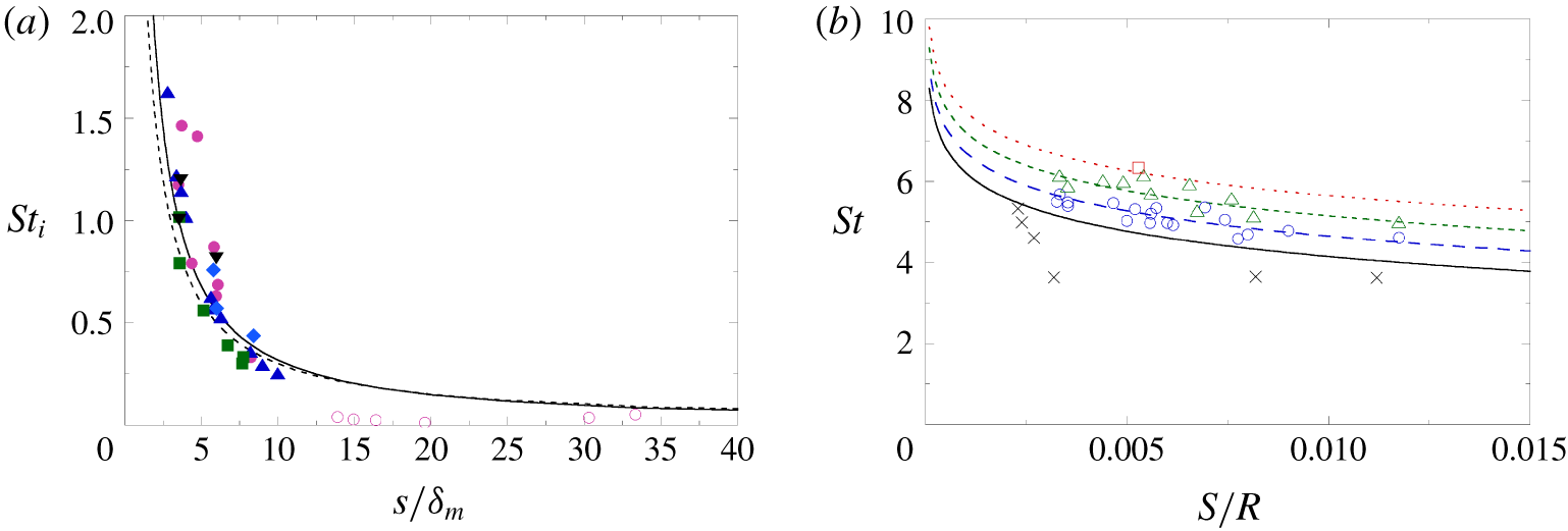
 ${\hat{s}}$ is shown in figure 6(a) in the experimental range
 $2\lesssim {\hat{s}}\lesssim 35$. It can be seen that the approximate hyperbolic prediction
 $St_{ic}\simeq 3/{\hat{s}}$ (dashed line) is not far from the complete prediction (solid line), with critical impact Stokes number in the range
 $0.1\lesssim St_{ic}\lesssim 1.5$. In figure 6(a) are also plotted all our experimental data where a microrebound is observed (filled symbols) or not (open symbols). As our measurements focused on the bouncing transition, most data points corresponding to bouncing are slightly above the theoretical line with only a few data points slightly below. The data corresponding to ‘sticking’ collisions are significantly below the theoretical line, which is quite satisfying.
(a) Impact Stokes  $St_{i}$ as a function of the ratio
 ${\hat{s}}=s/\unicode[STIX]{x1D6FF}_{m}$ of the hydrodynamic roughness
 $s$ relative to the sphere penetration depth
 $\unicode[STIX]{x1D6FF}_{m}$ for the experiments (data symbols of table 1) and theoretical predictions
 $St_{ic}=4\unicode[STIX]{x1D6FC}I$ with
 $\unicode[STIX]{x1D6FC}=0.9$ and equation (3.8) for
 $I$ (——) or equation (3.9) for
 $I$ (- - -) at large
 ${\hat{s}}$. Filled symbols correspond to bouncing cases whereas open symbols corresponds to non-bouncing cases. (b) Stokes number
 $St$ as a function of the hydrodynamic roughness/sphere size ratio
 $s/R$ for the experiments with open symbols when bouncing is observed for which
 $0.3\leqslant St_{ic}\leqslant 0.7$ (○),
 $0.8\leqslant St_{ic}\leqslant 1.2$ (▵), and
 $1.3\leqslant St_{ic}\leqslant 1.7$ (▫) and crosses (
 $\times$) when no bouncing is observed, together with theoretical prediction
 $St_{c}=\unicode[STIX]{x1D6FC}\ln (R/s)+St_{ic}$ with
 $\unicode[STIX]{x1D6FC}=0.9$ and
 $St_{ic}=0$ (——),
 $St_{ic}=0.5$ (– – –, blue),
 $St_{ic}=1$ (- - -, green) and
 $St_{ic}=1.5$ (
 $\cdots \,$, red).

The estimation for the critical value  $St_{c}$ of the global Stokes number can be written simply as
 $$\begin{eqnarray}St_{c}=St_{ic}\frac{V_{\infty c}}{V_{ic}}\simeq \unicode[STIX]{x1D6FC}\ln \left(\frac{R}{s}\right)+St_{ic}.\end{eqnarray}$$
In the above expression, the critical Stokes number appears as the sum of two terms: a first term arising from the viscous dissipation during the approach phase towards the array of micropillars; and a second term arising from viscous dissipation during the contact with the micropillars. The first term depends only on the coefficient  $\unicode[STIX]{x1D6FC}$ and the ratio
 $R/s$, thus on the micropillar array geometry and on the sphere size. The second term corresponds to the value of
 $St_{ic}$ discussed above. The theoretical evolution of the critical Stokes number
 $St_{c}$ as a function of
 $s/R$ is shown in figure 6(b) for
 $\unicode[STIX]{x1D6FC}=0.9$ and different
 $St_{ic}$ values from 0 to 1.5. As our experimental measurements focused on the bouncing transition, all our experimental data points are in a narrow range of Stokes number,
 $3.5\lesssim St\lesssim 6.5$. The data points for which a ‘sticking’ collision is observed (
 $\times$) are all below the solid line which delineates the transition. The other data points for which a (micro)rebound is observed appear here with different open data symbols depending on the range of
 $St_{ic}$. All these data points are close to the corresponding theoretical line.
4 The coefficient of restitution for the sphere–wall collision
We have seen that the sphere–wall collision process can be split into two parts: (i) the close approach of the sphere towards the micropillars; and (ii) the subsequent contact of the sphere with the pillars. This second part of the collision can be characterized by the ratio  $-V_{r}/V_{i}$ of the rebound velocity
 $V_{r}$ of the sphere when leaving the solid wall (at
 $h=0$) with respect to the impact velocity
 $V_{i}$ (at
 $h=0$). This ratio
 $-V_{r}/V_{i}$ can be derived considering that the rebound kinetic energy
 $E_{kr}=(1/2)M_{eff}V_{r}^{2}$ is just reduced from the initial kinetic energy
 $E_{ki}$ by the quantity
 $E_{d}$ from viscous dissipation during the collision, as the other force terms are conservative,
 $$\begin{eqnarray}\frac{-V_{r}}{V_{i}}=\left(1-\frac{E_{d}}{E_{ki}}\right)^{1/2}\simeq \left(1-\frac{St_{ic}}{St_{i}}\right)^{1/2}.\end{eqnarray}$$
When  $St_{i}<St_{ic}$, all the kinetic energy of the sphere is dissipated in the fluid during the contact so that no bouncing then occurs and the above expression is not valid. The bouncing and validity of (4.1) requires
 $St_{i}>St_{ic}$. For large impact Stokes number (
 $St_{i}\gg St_{ic}$), the velocity ratio reduces at first order to
 $-V_{r}/V_{i}=1-St_{ic}/2St_{i}$, whereas it reduces to
 $-V_{r}/V_{i}=(St_{i}/St_{ic}-1)^{1/2}$ for small impact Stokes number close to the bouncing/non-bouncing critical value
 $St_{ic}$ (
 $St_{i}\simeq St_{ic}$).
Note that the penetration distance is reduced by viscous dissipation. Considering an energy loss of approximately  $E_{d}/2$ with
 $E_{d}$ given by (3.7)–(3.8) corresponding to the first part of the contact from
 $\unicode[STIX]{x1D6FF}=0$ to
 $\unicode[STIX]{x1D6FF}_{m}$, the penetration distance
 $\unicode[STIX]{x1D6FF}_{m}$ is given by
 $$\begin{eqnarray}\frac{\unicode[STIX]{x1D6FF}_{m}}{\unicode[STIX]{x1D6FF}_{m0}}\simeq \left(1-\frac{St_{ic}}{2St_{i}}\right)^{1/3},\end{eqnarray}$$
where  $\unicode[STIX]{x1D6FF}_{m0}$ is the maximal penetration distance given by (3.6) for a non-dissipative collision. Far above the bouncing transition where the dissipation is small (
 $St_{i}/St_{ic}\gg 1$),
 $\unicode[STIX]{x1D6FF}_{m}$ is only slightly smaller than
 $\unicode[STIX]{x1D6FF}_{m0}$, and can be approximated by
 $\unicode[STIX]{x1D6FF}_{m}/\unicode[STIX]{x1D6FF}_{m0}\simeq 1-St_{ic}/6St_{i}$, with, e.g.
 $\unicode[STIX]{x1D6FF}_{m}/\unicode[STIX]{x1D6FF}_{m0}\simeq 0.98$ at
 $St_{i}/St_{ic}=10$. Closer to the bouncing transition where the dissipation is larger,
 $\unicode[STIX]{x1D6FF}_{m}$ is smaller but not so much, as
 $\unicode[STIX]{x1D6FF}_{m}/\unicode[STIX]{x1D6FF}_{m0}\simeq 2^{-1/3}\simeq 0.8$ at
 $St_{i}=St_{ic}$. The experimental penetration distance
 $\unicode[STIX]{x1D6FF}_{m}$ reported by CGM close to the bouncing transition varies between
 $0.5\unicode[STIX]{x1D6FF}_{m0}$ and
 $0.9\unicode[STIX]{x1D6FF}_{m0}$.
As both the velocity and the penetration distance are reduced by viscous dissipation, the evolution of the collision time is not so intuitive. Following the simple estimation of the typical time of collision  $\unicode[STIX]{x1D70F}_{0}\sim \unicode[STIX]{x1D6FF}_{m0}/V_{i}$ for a non-dissipative collision with the penetration distance
 $\unicode[STIX]{x1D6FF}_{m0}$ at the typical velocity
 $V_{i}$, the typical time of collision for a dissipative collision can be estimated as
 $\unicode[STIX]{x1D70F}_{v}\sim 2\unicode[STIX]{x1D6FF}_{m}/(V_{i}-V_{r})$ with the reduced penetration distance
 $\unicode[STIX]{x1D6FF}_{m}$ at the typical reduced velocity
 $(V_{i}-V_{r})/2$. From equation (4.1) for
 $-V_{r}/V_{i}$ and equation (4.2) for
 $\unicode[STIX]{x1D6FF}_{m}$, the collision time
 $\unicode[STIX]{x1D70F}_{v}$ for a dissipative collision writes as
 $$\begin{eqnarray}\frac{\unicode[STIX]{x1D70F}_{v}}{\unicode[STIX]{x1D70F}_{0}}\sim \frac{2\left(1-\displaystyle \frac{St_{ic}}{2St_{i}}\right)^{1/3}}{1+\left(1-\displaystyle \frac{St_{ic}}{St_{i}}\right)^{1/2}}.\end{eqnarray}$$
Far above the bouncing transition where the dissipation is small ( $St_{i}/St_{ic}\gg 1$),
 $\unicode[STIX]{x1D70F}_{v}$ can be approximated by
 $\unicode[STIX]{x1D70F}_{v}/\unicode[STIX]{x1D70F}_{0}\simeq 1+St_{ic}/12St_{i}$, and is thus only slightly larger than
 $\unicode[STIX]{x1D70F}_{0}$, e.g.
 $\unicode[STIX]{x1D70F}_{v}/\unicode[STIX]{x1D70F}_{0}\simeq 1.01$ at
 $St_{i}/St_{ic}=10$. Closer to the bouncing transition where the dissipation is larger,
 $\unicode[STIX]{x1D70F}_{m}$ is larger but does not diverge,
 $\unicode[STIX]{x1D70F}_{v}/\unicode[STIX]{x1D70F}_{0}\simeq 2^{2/3}\simeq 1.6$ at
 $St_{i}=St_{ic}$. The experimental collision times
 $\unicode[STIX]{x1D70F}_{v}$ reported by CGM close to the bouncing transition indeed varies between
 $\unicode[STIX]{x1D70F}_{0}$ and
 $1.6\unicode[STIX]{x1D70F}_{0}$. Note that Birwa et al. (Reference Birwa, Rajalakshmi, Govindarajan and Menon2018) also found an increase of the contact time for decreasing Stokes number close to their critical value
 $St_{c}\simeq 6$: the contact time of a smooth steel sphere colliding onto a smooth steel wall into a viscous silicon oil measured from their electrical set-up was observed to be constant for
 $1.3\lesssim St/St_{c}\lesssim 5$ and to increase abruptly very close to
 $St_{c}$ (
 $1\lesssim St/St_{c}\lesssim 1.3$), by a factor of
 $4\pm 2$.
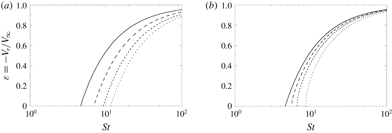
Theoretical restitution coefficient of the global collision process  $\unicode[STIX]{x1D716}=-V_{r}/V_{\infty }$ as a function of the global Stokes number
 $St$ from equation (4.6) for (a)
 $St_{ic}=0$ and
 $R/s=10^{2}$ (——),
 $10^{3}$ (– – –),
 $10^{4}$ (- - -) or
 $10^{5}$
 $(\cdots \,)$; and (b) for
 $R/s=10^{2}$ and
 $St_{ic}=0$ (——), 1 (– – –), 2 (- - -) or 4
 $(\cdots \,)$.

If we consider the whole collision process embedding not only the sphere–pillars contact but also the previous sphere approach close to the pillars, the global coefficient of restitution corresponds to the ratio  $\unicode[STIX]{x1D716}=-V_{r}/V_{\infty }$ of the rebound velocity
 $V_{r}$ to the typical approach velocity
 $V_{\infty }$. With the use of the macroscopic Stokes number
 $St=St_{i}V_{\infty }/V_{i}$ based on this approach velocity, the global coefficient of restitution is given by
 $$\begin{eqnarray}\unicode[STIX]{x1D716}=\frac{-V_{r}}{V_{i}}\frac{V_{i}}{V_{\infty }}\simeq \left(1-\frac{St_{ic}}{St}\frac{V_{\infty }}{V_{i}}\right)^{1/2}\frac{V_{i}}{V_{\infty }}.\end{eqnarray}$$
In equation (4.4),  $V_{i}/V_{\infty }$ is the velocity ratio corresponding to the approach phase, and gives from equation (3.2)
 $$\begin{eqnarray}\frac{V_{i}}{V_{\infty }}\simeq 1-\frac{\unicode[STIX]{x1D6FC}\ln (R/s)}{St}.\end{eqnarray}$$
Finally, the global coefficient of restitution  $\unicode[STIX]{x1D716}$ reduces (for
 $St\geqslant St_{c}$) to
 $$\begin{eqnarray}\unicode[STIX]{x1D716}\simeq \left(1-\frac{St_{ic}}{St-\unicode[STIX]{x1D6FC}\ln (R/s)}\right)^{1/2}\left(1-\frac{\unicode[STIX]{x1D6FC}\ln (R/s)}{St}\right),\end{eqnarray}$$
or
 $$\begin{eqnarray}\unicode[STIX]{x1D716}\simeq \left(1-\frac{St_{c}}{St}\right)^{1/2}\left(1-\frac{\unicode[STIX]{x1D6FC}\ln (R/s)}{St}\right)^{1/2}.\end{eqnarray}$$
Close to the bouncing transition, when  $St$ is only slightly larger than
 $St_{c}$, the coefficient of restitution is close to zero and can be approximated by
 $$\begin{eqnarray}\unicode[STIX]{x1D716}\simeq \frac{(St-St_{c})^{1/2}[St-\unicode[STIX]{x1D6FC}\ln (R/s)]^{1/2}}{St_{c}}.\end{eqnarray}$$
If one of the two dissipative processes can be neglected, the above expression can be simplified and leads to different scaling laws. Indeed, when  $St_{ic}\ll \unicode[STIX]{x1D6FC}\ln (R/s)$ the global coefficient of restitution reduces to
 $\unicode[STIX]{x1D716}\simeq St/St_{c}-1$ close to
 $St_{c}$, whereas it reduces to
 $\unicode[STIX]{x1D716}\simeq (St/St_{c}-1)^{1/2}$ when
 $St_{ic}\gg \unicode[STIX]{x1D6FC}\ln (R/s)$.
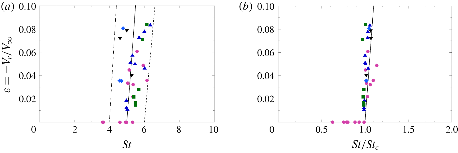
Restitution coefficient of the global collision process  $\unicode[STIX]{x1D716}=-V_{r}/V_{\infty }$ (a) as a function of the global Stokes number
 $St$ with experimental data (data symbols of table 1) and model equation
 $\unicode[STIX]{x1D716}=St/St_{c}-1$ for
 $St_{c}=4$ (– – –), 5 (——) and 6 (- - -); and (b) as a function of the reduced global Stokes number
 $St/St_{c}$.

The coefficient of restitution of the global collision process  $\unicode[STIX]{x1D716}$ predicted by equation (4.6) is plotted as a function of the global Stokes number
 $St$ in figure 7. In figure 7(a), the relative shift lengths
 $s/R$ are varied keeping
 $St_{ic}=0$, so that the critical Stokes number
 $St_{c}$ varies according to equation (3.11), and the
 $\unicode[STIX]{x1D716}(St)$ curve changes accordingly, but only with a global shift by keeping the same shape. Note that the set of curves of figure 7(a) is very similar to the set of
 $\unicode[STIX]{x1D716}(St)$ curves shown by Izard et al. (Reference Izard, Bonometti and Lacaze2014) for different relative sphere roughness. When the dissipation during the solid collision is taken into account in figure 7(b) at a constant
 $s/R=10^{-2}$, the critical Stokes number increases with increasing dissipation so that the
 $\unicode[STIX]{x1D716}(St)$ curve changes accordingly, here with no global shift but with a shape deformation. The two separate dissipation processes arising in the approach phase and in the solid contact have thus a very distinct influence on the
 $\unicode[STIX]{x1D716}(St)$ curve.
In figure 8(a), the global coefficient of restitution  $\unicode[STIX]{x1D716}$ is now plotted as a function of the global Stokes number
 $St$ for the experimental data together with the model equations corresponding to three different
 $St_{c}$ values:
 $St_{c}=4$, 5 and 6. As the experimental data are very close to the bouncing transition, the theoretical curves are very close to straight lines of equation
 $\unicode[STIX]{x1D716}=St/St_{c}-1$ for
 $St/St_{c}\geqslant 1$. The experimental data for which a rebound is observed (
 $\unicode[STIX]{x1D716}>0$) are within the band delimited by the two curves drawn for
 $St_{c}=4$ and 6, as we have already shown that
 $4.5\lesssim St_{c}\lesssim 6$ when bouncing is observed (figure 6b).
Finally,  $\unicode[STIX]{x1D716}$ is plotted in figure 8(b) as a function of the reduced Stokes number
 $St/St_{c}$. The experimental data are in the quite narrow range
 $0.6\lesssim St/St_{c}\lesssim 1.1$ around the critical transition value
 $St/St_{c}=1$. It is very satisfying that the data without bouncing (
 $\unicode[STIX]{x1D716}=0$) are observed to fall such as
 $St/St_{c}<1$, and that the data with bouncing (
 $\unicode[STIX]{x1D716}>0$) are quite close to the theoretical master curve of equation
 $\unicode[STIX]{x1D716}=St/St_{c}-1$ for
 $St/St_{c}\geqslant 1$. The bouncing transition is abrupt with a linear increase of
 $\unicode[STIX]{x1D716}$ with
 $St$ just above
 $St_{c}$.
5 Conclusion
The normal impact of a liquid-immersed sphere on a microtextured wall has been analysed taking into account the influence of viscous dissipation on the hydrodynamic and solid contact interactions between the sphere and the textured wall. The wall texture consists of an array of square micropillars. In our previous works, the separate effect of the texture geometrical parameters on the elastic contact force (Chastel et al. Reference Chastel, Gondret and Mongruel2016) and lubrication drag (Chastel & Mongruel Reference Chastel and Mongruel2019) had been assessed independently. Here, these effects are combined to yield a complete description of the collision process. An equation of motion for the sphere is proposed, describing its whole dynamics, that comprises the approach to the wall, the contact with the wall and also the subsequent rebound. As the wall textures reduce the lubrication pressure, the pillar deformation considered in the model does not result from the fluid pressure but from the solid contact force that arises when the sphere touches the top of the textures with a non-zero impact velocity. Experimental data previously obtained by high-frequency interferometry can be now entirely described by the modelling with a good agreement.
An analytical expression is derived for the critical Stokes number for bouncing,  $St_{c}$, that arises from the sum of two contributions corresponding to dissipation prior to and during the contact. Both contributions are strongly influenced by the geometrical parameters of the wall texture and the predictions are in agreement with the experimental data. An analytical expression is also derived for the coefficient of restitution
 $\unicode[STIX]{x1D716}$ as a function of the Stokes number
 $St$. The predicted linear evolution of
 $\unicode[STIX]{x1D716}$ with
 $St-St_{c}$ just above
 $St_{c}$ is found in good agreement with the experimental measurements.
The theoretical modelling developed in the present paper is for viscous fluids, i.e. when viscous dissipation from the interstitial fluid flow is much larger than all the other possible dissipation sources such as the viscoelasticity or plasticity of the solid materials or the excitation of vibrational modes.
These finding are useful for understanding precisely the influence of a surface roughness on the viscous dissipation in the near-wall bouncing dynamics. The methodology presented here could be extended to other surface roughness geometries. The present findings may also be useful for the implementation of realistic collisional models in numerical methods to simulate the flow of suspensions and liquid-immersed granular flows as in Biegert, Vowinckel & Meiburg (Reference Biegert, Vowinckel and Meiburg2017).
Acknowledgements
The authors wish to thank T. Chastel for measurements, A. Phor for data processing and J. Magnaudet for fruitful discussions. Suggestions from the referees are also gratefully acknowledged.
Declaration of interests
The authors report no conflict of interest.
Appendix A. Dependence of the near-field shift length $s$ upon the geometrical parameters of the textured wall

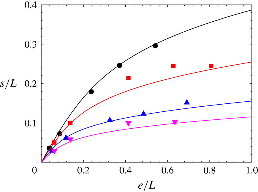
Evolution of the near-field shift length  $s$ normalized by the periodic spacing of the pillars
 $L$ as a function of the normalized height of the pillars
 $e/L$. Data symbols correspond to the experimental values from Chastel & Mongruel (Reference Chastel and Mongruel2019) for
 $\unicode[STIX]{x1D719}=0.05$ (●), 0.15 (▪), 0.30 (▴) and 0.45 (▾), and the solid lines correspond to equation (A 4) without any fitting parameters.

The near-field ( $h\ll L$) shift length
 $s$ used throughout the modelling has been measured by Chastel & Mongruel (Reference Chastel and Mongruel2019). Figure 9 illustrates how this parameter depends on the geometrical parameters of the pillar arrays. For a given value of pillar fraction
 $\unicode[STIX]{x1D719}$, the dimensionless shift length
 $s/L$ increases with dimensionless pillar height
 $e/L$. Smaller pillar fractions
 $\unicode[STIX]{x1D719}$ result in larger shift length values. In the following, we propose a correlation between
 $s/L$,
 $e/L$ and
 $\unicode[STIX]{x1D719}$, that is based on simple scaling arguments. First, in the limit of small pillar height (
 $e/L\ll 1$), far-field and near-field shift lengths must coincide, which yields a linear dependence with pillar height, with a slope increasing with decreasing
 $\unicode[STIX]{x1D719}$, (Chastel & Mongruel Reference Chastel and Mongruel2019)
 $$\begin{eqnarray}\frac{s}{L}=(1-\unicode[STIX]{x1D719})\frac{e}{L}.\end{eqnarray}$$
In the limit of large pillar heights ( $e/L\approx 1$), the viscous dissipation on the pillar lateral walls has to be taken into account. This can be done through a bilayer model (Seiwert et al. Reference Seiwert, Clanet and Quéré2011), in which the pillars and fluid around them are considered as a continuum of effective viscosity
 $\unicode[STIX]{x1D702}_{eff}=k\unicode[STIX]{x1D702}$, where
 $k$ is a dimensionless coefficient that depends on the geometrical parameters (
 $e/L$ and
 $\unicode[STIX]{x1D719}$) of the pillar array
 $$\begin{eqnarray}k=\frac{\unicode[STIX]{x1D702}_{eff}}{\unicode[STIX]{x1D702}}=1+\unicode[STIX]{x1D6FD}(\unicode[STIX]{x1D719})\left(\frac{e}{L}\right)^{2}\simeq \unicode[STIX]{x1D6FD}(\unicode[STIX]{x1D719})\left(\frac{e}{L}\right)^{2}.\end{eqnarray}$$
In the above equation, the coefficient  $\unicode[STIX]{x1D6FD}(\unicode[STIX]{x1D719})$ is related to the drag per unit length on a pillar in the array of pillars. This coefficient is an increasing function of
 $\unicode[STIX]{x1D719}$ which can be calculated by an analytical formula from Kuwabara (Reference Kuwabara1959):
 $\unicode[STIX]{x1D6FD}=13.8$, 36.2, 90.3, 107 for
 $\unicode[STIX]{x1D719}=0.05$, 0.15, 0.30, 0.45, respectively. In the bilayer model of Chastel & Mongruel (Reference Chastel and Mongruel2016), the radial pressure gradient in the squeeze flow between the sphere and the top of the pillars is found to have a similar form as in classical lubrication theory:
 $\text{d}p(r)/\text{d}r=-6\unicode[STIX]{x1D702}rV(h)/\bar{h}(r)$, where
 $\bar{h}(r)$ is a function of
 $e$,
 $k$ and
 $h+r^{2}/(2R)$. Thus,
 $\bar{h}(r)$ is a characteristic distance that yields the shift length as
 $s=\lim _{h\rightarrow 0}\bar{h}=e/k^{1/3}$, leading to the scaling law
 $$\begin{eqnarray}\frac{s}{L}\sim \left(\frac{e}{\unicode[STIX]{x1D6FD}(\unicode[STIX]{x1D719})L}\right)^{1/3}.\end{eqnarray}$$
An equation model based on the two limiting behaviours (A 1) and (A 3) can be built as
 $$\begin{eqnarray}\frac{s}{L}\simeq (1-\unicode[STIX]{x1D719})\left(\frac{e}{L}\right)\left[1+\unicode[STIX]{x1D6FD}(\unicode[STIX]{x1D719})\left(\frac{e}{L}\right)^{2}\right]^{-1/3}.\end{eqnarray}$$
It can be seen in figure 9 that the experimental values of  $s$ are quite well described by (A 4) over the whole range of geometrical parameters of the textures considered here.
Appendix B. On the possible elastohydrodynamic deformation
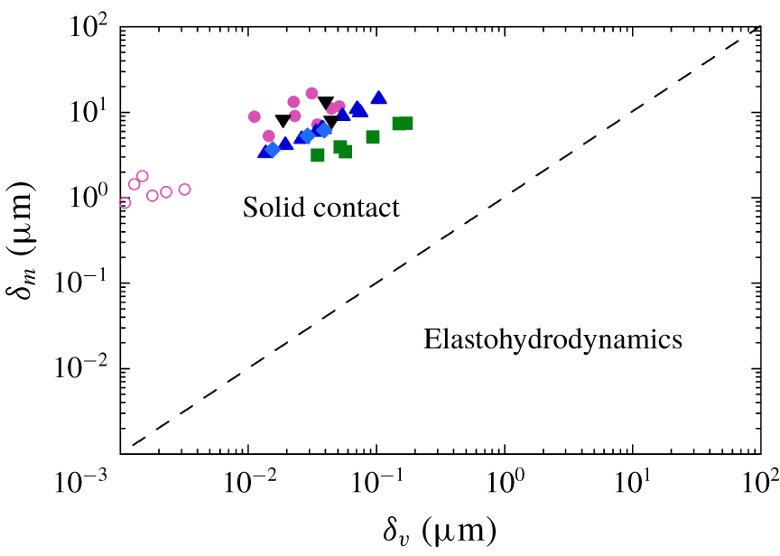
Measured sphere penetration depth  $\unicode[STIX]{x1D6FF}_{m}$ as a function of the estimated elastohydrodynamic deformation of pillars
 $\unicode[STIX]{x1D6FF}_{v}$ for all the experiments (data symbols of table 1 with filled (open) symbols for (non) bouncing case), together with the line of equation
 $\unicode[STIX]{x1D6FF}_{m}=\unicode[STIX]{x1D6FF}_{v}$ (- - -) delineating the domain of elastohydrodynamic deformation from the domain of deformation by solid contact.

In this appendix, we look at the possible elastohydrodynamic deformation. The lubrication force exerted on the sphere during its approach close to the wall textures is  $F_{D}=-6\unicode[STIX]{x03C0}R^{2}\unicode[STIX]{x1D702}V(h)/(h+s)$. This effective viscous force, which stems from the interaction of the sphere with the texture, results from an effective local pressure
 $p(h,r)=-3R\unicode[STIX]{x1D702}V(h)/(h+r^{2}/2R+s)^{2}$ that may lead to a possible deformation of the pillars. The maximum elastic deformation
 $\unicode[STIX]{x1D6FF}_{v}$ that would result from the maximal pressure
 $p(0,0)$ is
 $$\begin{eqnarray}\unicode[STIX]{x1D6FF}_{v}\simeq \frac{e}{E}p(0,0)\simeq \frac{3\unicode[STIX]{x1D702}eRV_{i}}{Es^{2}}.\end{eqnarray}$$
In the experiments considered here, this elastohydrodynamic deformation  $\unicode[STIX]{x1D6FF}_{v}$ would be typically between approximately 0.001 and
 $0.1~\unicode[STIX]{x03BC}\text{m}$, which is smaller, or of the order of, the microscopic roughness
 $\unicode[STIX]{x1D709}$ of the sphere surface and texture surface. Such an elastohydrodynamic deformation may thus be neglected and solid contact may be considered to happen at
 $h=0$. When neglecting gravity and any fluid effects, the elastic deformation from solid contact has been shown by CGM to be
 $$\begin{eqnarray}\unicode[STIX]{x1D6FF}_{m0}=\left(\frac{2\unicode[STIX]{x1D70C}_{s}eR^{2}V_{i}^{2}}{\unicode[STIX]{x1D719}E}\right)^{1/3}.\end{eqnarray}$$
The ratio of the two elastic deformations from either viscous or solid interaction is thus
 $$\begin{eqnarray}\frac{\unicode[STIX]{x1D6FF}_{v}}{\unicode[STIX]{x1D6FF}_{m0}}\simeq \frac{3\unicode[STIX]{x1D702}}{s^{2}}\left(\frac{\unicode[STIX]{x1D719}e^{2}RV_{i}}{2\unicode[STIX]{x1D70C}_{s}E^{2}}\right)^{1/3}.\end{eqnarray}$$
In the experiments considered here, this ratio is in the range  $0.001\lesssim \unicode[STIX]{x1D6FF}_{v}/\unicode[STIX]{x1D6FF}_{m0}\lesssim 0.02$ meaning that the elastohydrodynamic deformation is negligible when compared to the elastic deformation from solid contact. In the plot of figure 10 where the measured deformation
 $\unicode[STIX]{x1D6FF}_{m}$ is displayed as a function of the estimated elastohydrodynamic deformation
 $\unicode[STIX]{x1D6FF}_{v}$, one clearly sees that all the data points are well above the line
 $\unicode[STIX]{x1D6FF}_{m}=\unicode[STIX]{x1D6FF}_{v}$, thus in the domain of solid contact and not in the domain of elastohydrodynamics.
All the length scales embedded in the problem can be sorted as follows relative to the spatial resolution of the measurements,  $\unicode[STIX]{x1D6E5}\simeq 0.2~\unicode[STIX]{x03BC}\text{m}$
 $$\begin{eqnarray}\unicode[STIX]{x1D6FF}_{v}\lesssim \unicode[STIX]{x1D709}<\unicode[STIX]{x1D6E5}\ll \unicode[STIX]{x1D6FF}_{m}\ll s(e,b,L)\ll R.\end{eqnarray}$$
Appendix C. Time evolution of the difference force terms acting during the approach and collision of the sphere with the wall
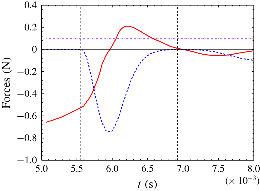
Model forces as a function of time for the case of figure 3(b) with  $2R=14~\text{mm}$,
 $\unicode[STIX]{x1D719}=0.05$,
 $2b=56~\unicode[STIX]{x03BC}\text{m}$ and
 $e=57~\unicode[STIX]{x03BC}\text{m}$. Viscous drag force
 $F_{D}$ (——), solid contact force
 $F_{w}$ (- - -), and apparent weight
 $F_{g}+F_{A}$ (— - —) of the immersed sphere. The two vertical dotted lines indicate the times of initial and final solid contact.

We look here at the time evolution of the different forces and their relative importance when the sphere is approaching and colliding with the wall. An example of such force evolution is shown in figure 11 for the case of figure 3(b) where the sphere bouncing is just small enough so that the sphere does not bounce off the wall. It thus corresponds to the data point where  $\unicode[STIX]{x1D716}=0$ at
 $St=St_{c}$ in figure 8(b). Before solid collision (
 $t\lesssim 5.5\times 10^{-3}~\text{s}$), the lubrication force
 $|F_{D}|$ is much larger than the apparent weight
 $|F_{g}+F_{A}|$, so that the sphere velocity decreases strongly. At the solid collision, the contact force
 $|F_{w}|$ increases strongly and reaches its maximum at
 $t\simeq 6\times 10^{-3}~\text{s}$, corresponding to the maximal penetration distance of the sphere where the sphere velocity is zero and the viscous drag is thus also zero. In the particular case of figure 11 corresponding to the critical Stokes number where the ‘rebound’ of the sphere is just
 $h=0$ at
 $t\simeq 7\times 10^{-3}~\text{s}$, the sphere then reaches its final static value for which the contact force just balances the apparent weight at
 $t\simeq 8\times 10^{-3}~\text{s}$.