2 The viscous simulation

We consider here the formation of the start-up vortex developing from the edge of a semi-infinite plate accelerating from rest in still air.

The viscous simulation was undertaken by solving the two-dimensional, incompressible, unsteady Navier–Stokes equations in their vorticity $\unicode[STIX]{x1D714}(x,y,t)$ , streamfunction $\unicode[STIX]{x1D713}(x,y,t)$ formulation.

The numerical scheme applied for the integration of the flow equations is described in detail in Luchini & Tognaccini (Reference Luchini and Tognaccini2002). Some information on the equations solved, on their boundary conditions and on the adopted non-dimensionalization are given in appendix A. The scheme is implicit and second-order accurate in both time and space variables. The number of unknowns was minimized by using an adaptive, unstructured grid of square cells. Indeed, grid points were introduced only in the region of non-negligible vorticity and the streamfunction, on the consequent time-dependent numerical boundary, is computed by using the Green integral. At each time step the convergence was accelerated by a multigrid algorithm properly adapted to the unstructured mesh. Moreover, in order to eliminate oscillations of the solutions near the edge of the plate (due to the locally large flow gradients), the multigrid integration scheme has been coupled with a local refinement of the grid. In this way the accuracy at the edge of the plate has been improved without the need to reduce the mesh size elsewhere.

The start-up vortex evolution is assumed to be initially characterized by a stage in which the flow is potential everywhere except for a thin Rayleigh-type viscous layer with constant thickness around the body (Xu & Nitsche (Reference Xu and Nitsche2015) conjectured that this stage does not strictly exist in the impulsive case, which is characterized by a recirculation region at the plate apex since an infinitely small time). Subsequently, the convective terms of the Navier–Stokes equations become comparable with viscous terms near the edge of the plate and a spiral vortex begins to form. When the convective terms become dominant the spiral vortex evolution enters in its self-similar stage in which the vortex is still small enough to be independent of the geometry except for the local wedge angle. Finally, the initial recirculation bubble opens up and the vortex starts lagging behind the body.

The simulation of the flow around a semi-infinite body allowed us to concentrate on the simulation of the self-similar stage of the vortex roll up. As already stated, all calculations, performed for both cases of impulsively starting plate and constant acceleration, revealed an unstable development of the vortex sheet. The perturbation amplified by the instability was not explicitly controlled, but introduced by the unavoidable truncation error of the numerical scheme. Despite this unpredictable random behaviour, the results obtained with different mesh sizes agreed in the description of the qualitative evolution of the instability and, quantitatively, in the determination of global variables, such as total circulation, vortex core position, vortex size and number of vorticity spots (‘cat-eyes’) present in the flow.

Two examples are illustrated in figure 1. These flows differ for the imposed start-up law. In particular, the cases of impulsive start-up to a constant speed and constant acceleration are shown. In the figure, two snapshots of the vorticity distributions are displayed. The cat-eyes spots are clearly visible, with a spiral vortex sheet still recognizable. Oscillations start near the plate apex and, subsequently, are convected towards the vortex core. The Reynolds number $Re_{S}$ specified in the figure caption was introduced by Pullin & Perry (Reference Pullin and Perry1980); due to the lack of a reference length it is strictly connected with the time variable:

where the dimensional constant $A$ depends on the imposed start-up velocity of the plate (see appendix A), $a$ is the time exponent of this law ( $a=0$ specifies impulsive start-up, $a=1$ constant acceleration start-up), $\unicode[STIX]{x1D708}$ is the kinematic viscosity and $m$ is related to the wedge angle $\unicode[STIX]{x1D6FD}=\unicode[STIX]{x03C0}(2-1/m)$ ( $m=1/2$ in the present case). It is noteworthy that in both simulations the instabilities became visible for $Re_{S}\approx 4500$ . For lower values of the Reynolds number the spirals showed a regular and smooth shape.

Figure 1.

Viscous simulations of the start-up vortex. Iso-curves of vorticity field $\overline{\unicode[STIX]{x1D714}}(\overline{x},\overline{y},\overline{t})$ ( $\unicode[STIX]{x0394}=15$ ) taken from Luchini & Tognaccini (Reference Luchini and Tognaccini2002). (a) Impulsive start-up ( $a=0$ ),  $Re_{S}=7713$ . (b) Constant acceleration start-up ( $a=1$ ),  $Re_{S}=7194$ .

The flow visualizations of Lepage et al. (Reference Lepage, Leweke and Verga2005) are impressively similar to the snapshots of figure 1 and confirmed the irregular evolution for large $Re_{S}$ values.

3 The inviscid simulation

In 1931, Kaden introduced similarity variables for describing the roll up of a semi-infinite plane vortex sheet, Saffman (Reference Saffman1992), p. 147. Pullin (Reference Pullin1978), for the first time, obtained regular and well-defined start-up vortex spirals from an accurate numerical solution of the integro-differential Birkhoff–Rott equation (inviscid flow) written in similarity variables. In self-similar coordinates the spiral vortex shape comes out time independent and the total circulation remains constant.

The attempt to simulate the start-up vortex evolution by an unsteady inviscid lumped-vortex method is not new, see Sarpkaya (Reference Sarpkaya1989) for instance. Many authors reported stability problems of their algorithms and were not able to obtain a smooth and regular evolution of the spiral vortex comparable with the self-similar solution of Pullin. Krasny (Reference Krasny1991) proposed a qualitative satisfactory comparison of an inviscid time-dependent solution with Pullin’s results by looking at the early evolution of the wake shedding from an impulsively accelerated plate of finite length. Using a vortex blob method, he presented smooth roll ups of the vortex in agreement with Pullin’s solution in terms of size and shape of the spiral. Calculations were repeated using blobs of different size. Nonetheless, in the most refined simulation the adopted blob diameter was still ${\approx}10\,\%$ of the total size of the vortex spiral; therefore, the possibility that Pullin’s solution might be obtained by the time evolution of a vortex sheet with infinitely small thickness requires further analysis. The adoption of a blob of finite thickness is equivalent to the introduction of an ‘artificial’ viscosity in the numerical scheme. An ‘equivalent’ Reynolds number can be determined by imposing that the blob diameter is comparable with the thickness of the viscous vortex sheet, a measure of which can be given by the Rayleigh layer thickness (see appendix A). The results of Krasny obtained with the smallest blobs were equivalent to $Re_{S}\approx 1000$ ; hence it is possible that, in Krasny’s calculations, the numerical viscosity artificially stabilized the spiral evolution (in our viscous calculations the instability evidenced for $Re_{S}>4500$ ). Indeed, subsequently, Krasny & Nitsche (Reference Krasny and Nitsche2002) verified that this regular evolution is limited to a finite time interval by simulating the start-up of a finite two-dimensional vortex sheet and an axisymmetric vortex ring. By decreasing the blob diameter the instability appeared sooner (in agreement with our description of the phenomenon by an ‘artificial’ Reynolds number) and the authors proposed that the appearance of the irregularities is a converged result with respect to mesh refinement in the spatial and temporal discretization. In analogy with the oscillating vortex pair model they related these features to the onset of chaos in the dynamic system induced by self-sustained oscillations and not by external forcing.

By a very similar method and with much smaller blobs we performed the simulation of the vortex shedding from a semi-infinite plate. The spiral is modelled by $N$ point vortices with intensity $\unicode[STIX]{x1D6E4}_{p}$ . Their evolution is computed solving the unsteady Euler equations written in inviscid self-similar variables by a Runge–Kutta method. The velocity field is analytically computed adding to the streamfunction of the wedge flow of 0 angle the fields induced by the point vortices. The boundary condition at the plate wall is enforced by appropriate image vortices. At each time step a vortex at the plate apex is added and its intensity is computed imposing the Kutta condition of finite velocity at the trailing edge. In order to keep the number of vortices $N$ constant the two oldest vortices in the core of the spiral are merged. Details on the equation solved and on the numerical method are given in appendix B.

Our unsteady inviscid simulations in self-similar variables show a very irregular time evolution and, as in Sarpkaya and Krasny’s attempts, do not reach the time-independent regular spiral vortex shape obtained by Pullin. The computations were run until the solution reached a statistically steady state (in the sense that integral quantities such as the total vorticity ceased to drift). Two snapshots of the solutions thus obtained in the self-similar plane are shown in figure 2, for both cases of impulsive and constant acceleration start-up. In the picture the radius of each displayed circle is proportional to the intensity of the corresponding point vortex. Their distribution is randomly oscillating about a recognizable spiral structure. Despite these random motions, an ‘average’ self-similarity exists because, measured in similarity variables, the size of the spiral (see appendix B for the definition of the similarity plane $\unicode[STIX]{x1D701}=\unicode[STIX]{x1D709}+\text{i}\unicode[STIX]{x1D702}$ , $\text{i}=\sqrt{-1}$ ) does not change with self-similar time $T$ . In addition, the total circulation obtained summing the intensity of each point vortex ( 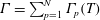$\unicode[STIX]{x1D6E4}=\sum _{p=1}^{N}\unicode[STIX]{x1D6E4}_{p}(T)$ ) also does not exhibit any noticeable oscillation with time.

Figure 2.

Inviscid unsteady simulation. Snapshots of the vortex spirals computed by the unsteady lumped-vortex method. $\unicode[STIX]{x0394}T=0.003$ ; $N=2000$ ; number of time steps $=10\,000$ . The radius of the circles is proportional to the vortex intensity. (a) Impulsive case ( $a=0$ ). (b) Constant acceleration case ( $a=1$ ).

The regular solutions of the Birkhoff–Rott equation found by Pullin (Reference Pullin1978) were re-obtained by constraining the inviscid problem through a Newton–Raphson algorithm (see appendix B), they are shown in figure 3. Interestingly enough, the size of the vortex spirals, the total circulation $\unicode[STIX]{x1D6E4}$ and the vortex core position $\unicode[STIX]{x1D701}_{c}=\unicode[STIX]{x1D709}_{c}+\text{i}\unicode[STIX]{x1D702}_{c}$ ( $\unicode[STIX]{x1D701}_{c}=\sum _{p=1}^{N}\unicode[STIX]{x1D701}_{p}\unicode[STIX]{x1D6E4}_{p}(T)/\unicode[STIX]{x1D6E4}$ ) are in agreement with the results obtained by the unsteady simulations.

Table 1 shows that, for the case $a=0$ , there are variations smaller than 3 % for $\unicode[STIX]{x1D6E4}$ , while they are 8 % in terms of $\unicode[STIX]{x1D701}_{c}$ . In the case $a=1$ , the variations are smaller than 0.5 % for both $\unicode[STIX]{x1D6E4}$ and $\unicode[STIX]{x1D701}_{c}$ . The differences, more significant for the case $a=0$ , are due to the reduced number of the lumped vortices employed in the computation of Pullin’s solutions. Indeed, in figures 4 and 5  $\unicode[STIX]{x1D6E4}$ and $\unicode[STIX]{x1D701}_{c}$ are plotted versus the number of adopted lumped vortices for both the steady and unsteady simulations and for both cases $a=0$ and $a=1$ . $\unicode[STIX]{x1D6E4}$ and $\unicode[STIX]{x1D701}_{c}$ are converging as the number of vortices $N$ is increased, however the convergence is slower for the impulsive case $a=0$ (in both steady and unsteady simulations) and the most refined simulation of the steady vortex spiral ( $N=300$ ) is still not sufficient to get the converged result.

Figure 3.

Solutions of the Birkhoff–Rott equation. The radius of the circles is proportional to the vortex intensity. (a) Impulsive case ( $a=0$ ),  $N=160$ . (b) Constant acceleration case ( $a=1$ ),  $N=200$ .

Table 1.

$\unicode[STIX]{x1D6E4}$ and $\unicode[STIX]{x1D701}_{c}$ obtained by inviscid lumped-vortex calculations with different numbers of point vortices; case $a=0$ , $\unicode[STIX]{x0394}T=0.003$ . Last column specifies the regularized computation of Pullin’s solution ( $N=300$ , $\unicode[STIX]{x0394}T=0.003$ ).

Table 2.

$\unicode[STIX]{x1D6E4}$ and $\unicode[STIX]{x1D701}_{c}$ obtained by inviscid lumped-vortex calculations with different numbers of point vortices; case $a=1$ , $\unicode[STIX]{x0394}T=0.003$ . Last column specifies the regularized computation of Pullin’s solution ( $N=200$ , $\unicode[STIX]{x0394}T=0.005$ ).

Figure 4.

Total circulation versus number of lumped vortices for the impulsive ( $a=0$ ) and constant acceleration ( $a=1$ ) inviscid start-up. Solid line: solution of Birkhoff–Rott equation; dashed line: unsteady simulation $\unicode[STIX]{x0394}T=0.003$ .

Figure 5.

Vortex core position versus number of lumped vortices for the impulsive ( $a=0$ ) and constant acceleration ( $a=1$ ) inviscid start-up. Solid line: solution of Birkhoff–Rott equation; dashed line: unsteady simulation $\unicode[STIX]{x0394}T=0.003$ .

The irregular inviscid solutions have been analysed in terms of the total circulation $\unicode[STIX]{x1D6E4}$ , of $\unicode[STIX]{x1D701}_{c}$ and of the position, along the spiral, where the instability becomes visually identifiable.

The number of lumped vortices $N$ and $\unicode[STIX]{x0394}T$ , the time step adopted in the calculations, are the only numerical parameters required. The effect of $N$ is evidenced in tables 1 and 2. $\unicode[STIX]{x1D6E4}$ and $\unicode[STIX]{x1D701}_{c}$ are rapidly converging as $N$ increases (for the case $a=1$ the results are practically converged even in the coarsest simulation). The influence of $\unicode[STIX]{x0394}T$ is evidenced in figure 6, where the vortex spirals are shown for $\unicode[STIX]{x0394}T=0.003$ and $\unicode[STIX]{x0394}T=0.001$ ( $N=1000$ , $a=1$ ). As $\unicode[STIX]{x0394}T$ decreases there is an expected loss of resolution near the vortex core, but, more interesting, the starting point of the instability moves towards the plate apex: it is therefore very likely that the instability of the inviscid numerical simulation starts right at the trailing edge for infinitely small $\unicode[STIX]{x0394}T$ .

Figure 6.

Vortex spirals computed by the unsteady lumped-vortex method. Effects of $\unicode[STIX]{x0394}T$ . Constant acceleration case ( $a=1$ );  $N=1000$ ; number of time steps $=10\,000$ . The radius of the circles is proportional to the vortex intensity. (a) $\unicode[STIX]{x0394}T=0.003$ ; (b) $\unicode[STIX]{x0394}T=0.001$ .

4 Comparison of the viscous and inviscid vortex spirals

There are interesting common features in the unstable viscous solutions and in the inviscid irregular blob distributions. Nevertheless a careful quantitative analysis is required to really appreciate if, as time grows, the Navier–Stokes solution converges towards the inviscid result.

In figure 7 the time histories of the instantaneous total circulations $\unicode[STIX]{x1D6E4}(\overline{t})$ are plotted for $a=0$ and $a=1$ , as determined by the Navier–Stokes simulations. $\unicode[STIX]{x1D6E4}$ is given by

where $\unicode[STIX]{x1D6FA}(\unicode[STIX]{x1D709},\unicode[STIX]{x1D702},T)$ is the vorticity in inviscid similarity variables. The relationship between the self-similar and viscous variables is given by (see also appendices A and B):

where $\overline{z}=\overline{x}+\text{i}\overline{y}$ . The self-similarity of the Navier–Stokes solution for large values of time is confirmed by this plot: $\unicode[STIX]{x1D6E4}(\overline{t})$ does approach the asymptotic inviscid value.

Figure 7.

Total circulation versus time for the impulsive ( $a=0$ ) and constant acceleration ( $a=1$ ) start-up. Solid lines: viscous simulation taken from Luchini & Tognaccini (Reference Luchini and Tognaccini2002). Dotted lines: inviscid solution ( $N=2000$ ).

The time histories of the vortex core coordinates $\unicode[STIX]{x1D709}_{c}$ , $\unicode[STIX]{x1D702}_{c}$ ( $a=0$ ) are reported in figure 8, with the instantaneous position of the viscous vortex core determined by the relation:

There is again a reasonable concordance with the inviscid results, even more so in the case $a=1$ where $\unicode[STIX]{x1D701}_{c}$ has practically reached its asymptotic value.

Figure 8.

Vortex core position versus time. Solid lines: viscous simulation taken from Luchini & Tognaccini (Reference Luchini and Tognaccini2002). Dotted lines: inviscid solution ( $N=2000$ ). (a) Impulsive start-up ( $a=0$ ); (b) constant acceleration start-up ( $a=1$ ).

The shapes of the spiral vortices can be compared in the plane of the inviscid self-similar coordinates. An example is given in figure 9 for the case $a=1$ . In the figure the iso-curves of the time-averaged vorticity $\overline{\unicode[STIX]{x1D6FA}}$ in the $\unicode[STIX]{x1D701}$ plane are displayed (only positive values of vorticity are plotted). The instantaneous vorticity of the unsteady inviscid solution has been obtained by sampling the domain on a square grid of mesh size $h_{s}=0.005$ and computing the vorticity in each sampled cell ( $i,j$ ) by the relation:

where the summation is taken over the $N_{c}$ vortices that at time $T$ are inside the sampling cell ( $i,j$ ). $\overline{\unicode[STIX]{x1D6FA}}$ has been computed by the relation

and turned out to be independent of the time interval ( $t_{i},t_{f}$ ) if a sufficiently high number of time steps was used in the numerical simulation.

The viscous averages have been computed from the solutions corresponding to the medium sized test (mesh size $h=0.2$ ), the ones that reached the largest time values in Luchini & Tognaccini (Reference Luchini and Tognaccini2002) and sampling the data in the same grid, characterized by $h_{s}=0.005$ , where the inviscid data had been taken. The size and shape of the average viscous spirals were also revealed to be independent of the used time interval and were in impressive agreement with the average inviscid spirals. Nonetheless, it should be said that the time intervals used in the Navier–Stokes simulations were not sufficiently large to achieve an asymptotically steady distribution of $\overline{\unicode[STIX]{x1D6FA}}$ .

Figure 10(a) presents the distribution of the average vorticity of $\overline{\unicode[STIX]{x1D6FA}}(\unicode[STIX]{x1D709})$ , in the case of viscous flow, plotted along the line $\unicode[STIX]{x1D702}=\unicode[STIX]{x1D702}_{c}$ (case $a=0$ ) with different intervals of time averaging as specified in the caption. Figure 11(a) presents the same data obtained by the inviscid simulations for different values of $N$ . The same results are presented for the case $a=1$ in figures 12(a) and 13(a).

Figure 9.

Iso-curves ( $\unicode[STIX]{x0394}=20$ ) of average vorticity $\overline{\unicode[STIX]{x1D6FA}}(\unicode[STIX]{x1D709},\unicode[STIX]{x1D702})$ in the inviscid self-similar plane; impulsive start-up $a=1$ . (a) Viscous solution, $\overline{t}_{i}=1720$ , $\overline{t}_{f}=2100$ ; (b) inviscid solution, $N=2000$ , $\unicode[STIX]{x0394}T=0.003$ .

Although the average vorticity of the Navier–Stokes solutions did not reach an asymptotic distribution, it does appear to move towards the inviscid one (more evidently in the case of $a=1$ ), in particular the peaks of the viscous simulations are still increasing and are tightening. Moreover, in order to complete the analysis of the inviscid results, it is interesting to note that the inviscid average vorticity distribution converges as $N\rightarrow \infty$ (much faster for $a=1$ ).

Figure 10.

Impulsive start-up ( $a=0$ ), viscous solution. (a) $\overline{\unicode[STIX]{x1D6FA}}$ versus $\unicode[STIX]{x1D709}$ ; (b) $\unicode[STIX]{x1D70E}_{\unicode[STIX]{x1D6FA}}$ versus  $\unicode[STIX]{x1D709}$ . ♢: $\overline{t}_{i}=900$ , $\overline{t}_{f}=1040$ ; $+$ : $\overline{t}_{i}=1040$ , $\overline{t}_{f}=1320$ ; ▫: $\overline{t}_{i}=1320$ , $\overline{t}_{f}=1620$ .

Figure 11.

Impulsive start-up ( $a=0$ ), inviscid solution, $\unicode[STIX]{x0394}T=0.003$ . (a) $\overline{\unicode[STIX]{x1D6FA}}$ versus $\unicode[STIX]{x1D709}$ ; (b) $\unicode[STIX]{x1D70E}_{\unicode[STIX]{x1D6FA}}$ versus $\unicode[STIX]{x1D709}$ . ♢: $N=500$ ; $+$ : $N=1000$ ; ▫: $N=1500$ ; $\times$ : $N=2000$ .

Despite these promising results, to enforce the interpretation of the ‘irregular’ inviscid vortex spiral as the asymptotic solution of the Navier–Stokes simulation we performed a further analysis. In fact, an agreement of the average solution is not sufficient to draw such a conclusion. To strengthen the result, a comparison of the standard deviation of the instantaneous vorticity distribution may be useful. The standard deviation of the vorticity distribution:

is plotted in figures 10(b), 11(b), 12(b) and 13(b) for the viscous and inviscid simulations and for the cases $a=0$ and $a=1$ respectively. Again, in both cases $a=0$ (figure 11 b) and $a=1$ (figure 13 b), the inviscid results converge for $N\rightarrow \infty$ .

Figure 12.

Constant acceleration start-up ( $a=1$ ), viscous solution. (a) $\overline{\unicode[STIX]{x1D6FA}}$ versus $\unicode[STIX]{x1D709}$ ; (b)  $\unicode[STIX]{x1D70E}_{\unicode[STIX]{x1D6FA}}$ versus $\unicode[STIX]{x1D709}$ . ♢: $\overline{t}_{i}=600$ , $\overline{t}_{f}=920$ ; $+$ : $\overline{t}_{i}=1115$ , $\overline{t}_{f}=1520$ ; ▫: $\overline{t}_{i}=1720$ , $\overline{t}_{f}=2100$ .

Figure 13.

Constant acceleration start-up ( $a=1$ ), inviscid solution, $\unicode[STIX]{x0394}T=0.003$ . Distributions of $\overline{\unicode[STIX]{x1D6FA}}(\unicode[STIX]{x1D709})$ and $\unicode[STIX]{x1D70E}_{\unicode[STIX]{x1D6FA}}(\unicode[STIX]{x1D709})$ ; case $a=1$ . (a) $\overline{\unicode[STIX]{x1D6FA}}$ versus $\unicode[STIX]{x1D709}$ ; (b) $\unicode[STIX]{x1D70E}_{\unicode[STIX]{x1D6FA}}$ versus $\unicode[STIX]{x1D709}$ . ♢: $N=500$ ; $+$ : $N=1000$ ; ▫: $N=2000$ .

As could be expected, the peaks of the standard deviation correspond to the turns of the vortex spiral. Looking at the time evolution of $\unicode[STIX]{x1D70E}_{\unicode[STIX]{x1D6FA}}$ in the Navier–Stokes solutions (figure 10 b for the case $a=0$ and figure 12 b for $a=1$ ) one can see the formation of the peaks along the outermost spiral turn; on the other hand, in the core the values of $\unicode[STIX]{x1D70E}_{\unicode[STIX]{x1D6FA}}$ are still very small compared to the inviscid values. This can be explained since the instabilities start to appear in the form of Kelvin–Helmholtz-like vorticity spots along the first spiral turn evolving from the edge of the plate; only afterwards do the spots form in the inner turns and cause the oscillations in vorticity distribution evidenced by the inviscid peak values of $\unicode[STIX]{x1D70E}_{\unicode[STIX]{x1D6FA}}$ . It should be said that all the Navier–Stokes numerical simulations, even the ones with larger mesh size, were stopped while the spots were still far from the vortex core: oscillations very near the vortex core are not present but these are likely to appear at a later stage.

In conclusion, the results of the comparison can be summarized as follows:

1. (i) the spiral shape of the average vorticity distributions obtained in the viscous and inviscid simulations are in agreement when compared in inviscid self-similar variables;

2. (ii) the average vorticity distribution of the Navier–Stokes simulation tends towards the inviscid one, the total circulation and core position do as well;

3. (iii) the instabilities start at the edge of the plate in both the viscous and inviscid solutions;

4. (iv) the standard deviations of the instantaneous vorticity distributions from the average value are in reasonable in agreement for $t\rightarrow \infty$ .